1. Introduction
Canopy structure is the vertical and horizontal distribution of plant material in a forested ecosystem and is a driver of many ecosystem functions and processes. Canopy structure influences the distribution of photosynthetic material and its efficiency [
1], microclimate [
2], stand species dynamics [
3], energy balances [
4], and species habitat and behavior [
5]. Similarly, forest fluid dynamics are closely tied to forest structure, including atmospheric flow within forests [
6] as well as the redistribution of intercepted precipitation [
7].
In the case of wildland fire, canopy structure influences the fire dynamics directly as fuel and indirectly through its influence on other variables in the fire environment. For example, three-dimensional fuel structure has been shown to have an influence on fuel moisture regimes, with the forest floor being consistently more moist under dense canopies [
8,
9]. Structure also influences the fire environment, or factors affecting the dynamics of the fire, by influencing wind and energy flow through drag [
10] and energy absorption [
11]. Likewise, models of smoke dispersion through variable canopy architecture allow the prediction of potential smoke dispersion patterns and thus increase knowledge of the degree to which canopy architecture influences forest level air parcel movement [
12,
13]. As an assemblage of fuel elements, the canopy directly contributes to the dynamics of wildland fires, including rate of spread and energy release [
14,
15]. Canopy fuels are thus not only vital to understanding fire spread and behavior [
16], they are also inputs in both empirical [
17] and computational fluid dynamics (CFD; [
18]) models of wildland fire behavior.
Fire severity is a measure of the change in the properties of the surface and vegetation resulting from a fire event [
19]. Fire severity varies greatly within and among burns in both vertical and horizontal dimensions, resulting in a complex landscape-wide mosaic of forest structure and composition [
20]. Integrating measurements of forest structure from before and after a fire incorporates the full spatial dimensionality of terrestrial fire effects (note that some first and second order fire effects may occur below ground) that are directly relatable to management needs and ecological function in forests.
Field-based estimates of fire severity such as the Composite Burn Index (CBI; [
21]) are often qualitative, relying on ocular estimates of “change” in various fuel strata, e.g., forest floor, shrubs, and canopies. A major confounding factor in CBI as a metric is that it does not consider pre-fire data, which can lead to the misattribution of an effect that was not actually due to the fire [
22]. For example, McCarley et al. [
23] illustrated the importance of considering pre-fire canopy structures with an example where the interaction of the effects of mountain pine beetle and severe wildfire reduced canopy cover more than severe wildfire alone. In this case, without the benefit of pre-fire data, CBI would have attributed these effects to the fire. Additionally, while CBI can be useful for estimating fire effects statistics for units on a landscape, they are poorly resolved spatially, can suffer from subjectivity, and have limitations for use in fire modeling or examining landscape pattern [
24].
Fire severity can be effectively indexed using remote sensed spectral reflectance data at large scales and increasingly high resolutions [
25,
26,
27]. The advantages of remote sensing analyses include the potential to map the entire spatial extent of a fire or region, and the potential to incorporate both before-fire and after-fire information. Furthermore, the increased availability of multi-temporal datasets has led to an increased understanding of spatial patterning and recovery through disturbance cycles. In many cases, studies have focused on post-fire landscape matrices by examining two-dimensional estimations of fire-severity, mostly derived from Landsat datasets [
28,
29]. These data are useful for operational purposes, chiefly to assess the spatial need for post-fire mitigation activities [
24]. However, these spectral reflectance-derived indices are only useful for developing a two-dimensional understanding of severity analogs and are not suited for measuring forest structural variables in three-dimensions. Problematically, these estimates only provide an index of fire severity, as they are not a direct measurement of the changes in the fuel strata [
30].
Characterization of forest structure, and the changes following fire, would therefore greatly enhance the understanding of fire severity. However, the field-based estimation of forest structural attributes can only be quantified in the field at very limited scales. First, field assessments of post-fire environments can be dangerous and difficult to access, limiting the potential spatial resolution and investment toward field collected data. Additionally, direct measures of structural attributes are challenging because of the difficulty in accessing the canopy. Thus, canopy structure attributes are typically inferred by models using measurements of stem height, stem diameter, and crown base height as inputs for species-specific models of canopy fuels distributions [
31]. This approach is problematic in the context of fire effects on canopies. Pre-determined distributions typically used to populate canopy fuels can be insensitive to the heterogeneity typical of canopy structure. More importantly, in the case of non-stand replacing fires, stem height, stem diameter, and crown base height do not change appreciably even after changes in canopy architecture have occurred. This is particularly problematic in stands composed of species that resprout epicormically, where foliar elements of the canopy are completely consumed and then can grow back from the same stem. However, these plot-based estimates do provide vital input parameters for the development of models that scale measurements using remote sensing datasets.
Forest structural attributes can now be quantified using Light Detection and Ranging (LiDAR) sensors, which make three-dimensional measurements of the forest that can be analyzed in ways that are directly applicable to wildland fire science [
32,
33,
34]. Using LiDAR, it is now possible to represent forest structure at the plot scale using Terrestrial Laser Scanning (TLS), at the landscape scale using Airborne Laser Scanning (ALS), and at the global scale using space-born laser sensors. Because ALS data can be collected at a scale and resolution that can encompass large fire perimeters, it is particularly well suited for providing structural fire effects data. Analysis approaches that leverage the full potential of these datasets can offer new insight into the alteration of forest function and processes due to disturbances. Voxel-based approaches for binning ALS returns into discrete height categories can preserve the structural information present in the ALS dataset that is otherwise lost in approaches that only make use of distributional statistics [
35]. This information presents a direct representation of the horizontal and vertical distribution of fuels. Given that these attributes of structure are vital for improving our understanding of many aspects of forest ecology, particularly the behavior and effects of wildland fire, it is important to develop and demonstrate new analytical methods to extract more informative structural information about forest vegetation matrices. Additionally, pre- and post-fire LiDAR data has been shown to accurately estimate forest structural changes across landscapes in several cases. Exploring fire severity in three continuous dimensions via remotely sensed forest structure datasets as a change from a pre-fire condition, has received limited previous attention; however, such an approach is posed to facilitate robust analyses of pyrogenic landscapes in ways that expand our understanding of the dynamics of fire effects on forest structure in the context of both wildland and prescribed fire, as well as the ecological nuances of fire regimes.
The objectives of this study were: (1) to investigate whether pre-fire canopy structure influenced fire severity; (2) to examine how vertical structural heterogeneity was modified across a gradient of fire severities; and (3) to describe landscape-scale changes in spatial patterning of forest structure resulting from fire. To work towards these objectives, we decomposed the influence of pre-fire forest structure characteristics on fire severity and subsequent changes in post-fire canopy structure using a combination of active and passive remote sensing datasets. We simplified pre- and post-ALS datasets using a classification strategy that more effectively preserves information about three-dimensional forest structure heterogeneity than current commonly used approaches. Next, we used a previously published map of burn severity to stratify the classified ALS data and allow us to identify trends and patterns in these datasets. The intersection of the pre-fire fuel structure, fire severity, and post-fire fuel structure data products allowed us to directly address the objectives set forth above.
4. Discussion and Conclusions
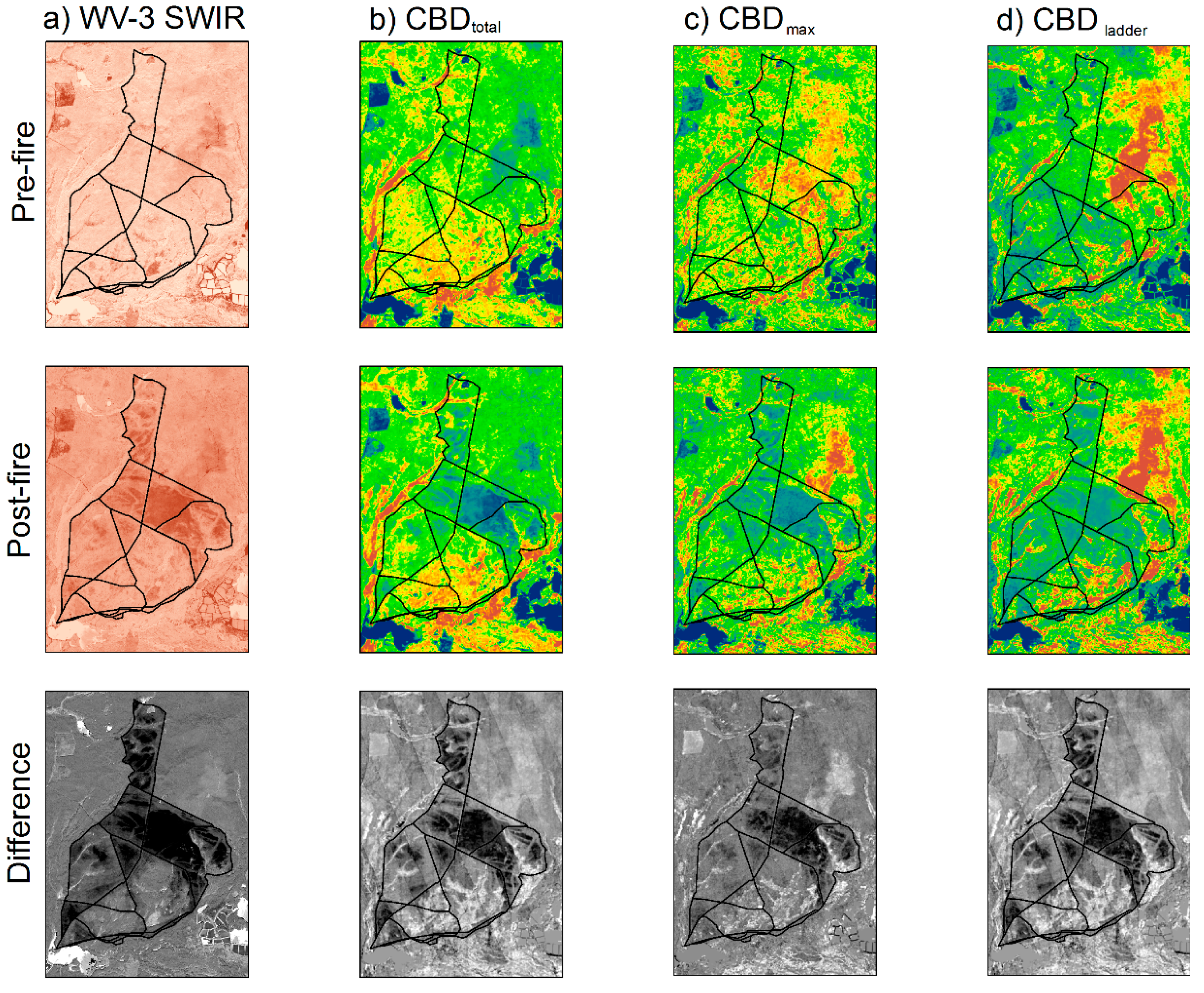
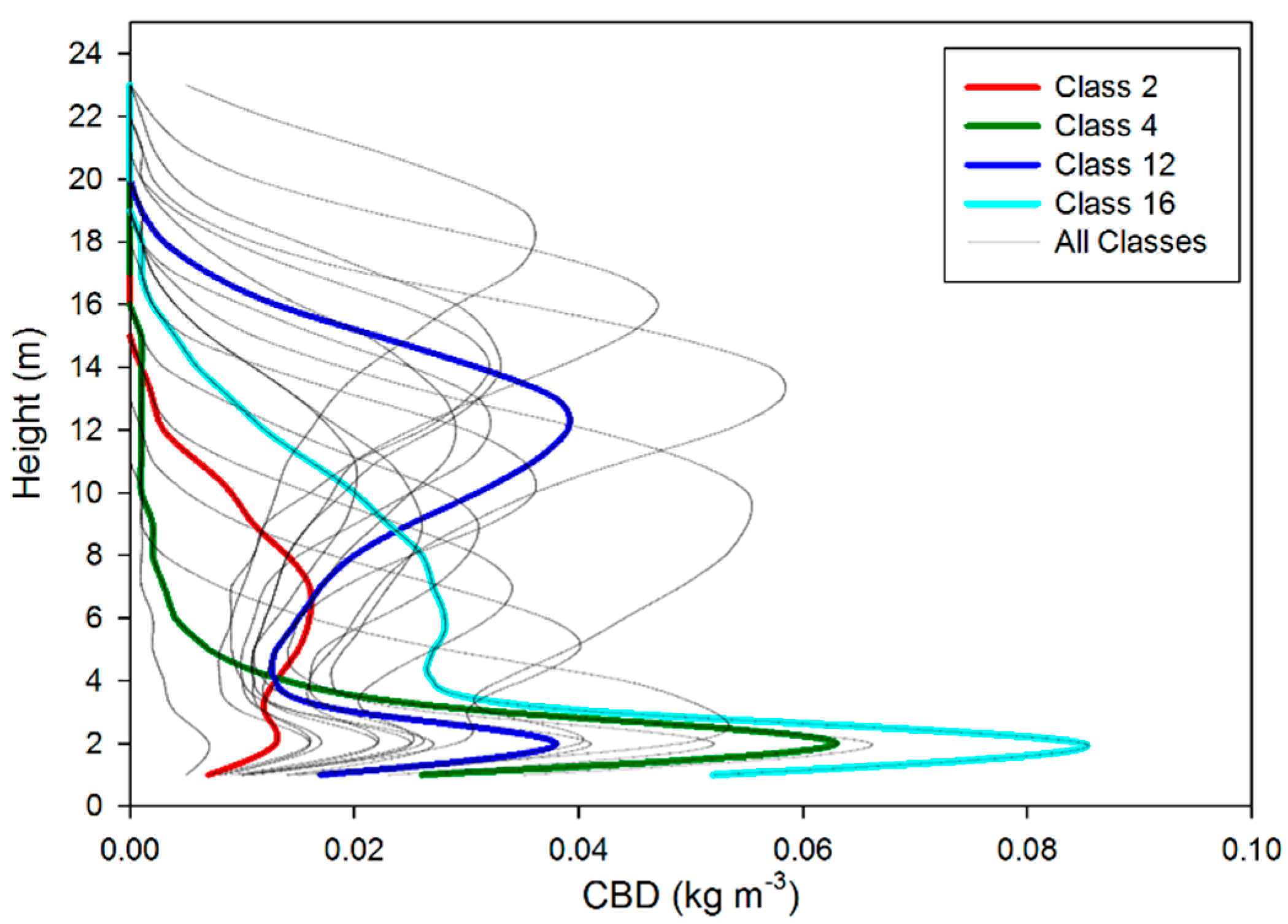
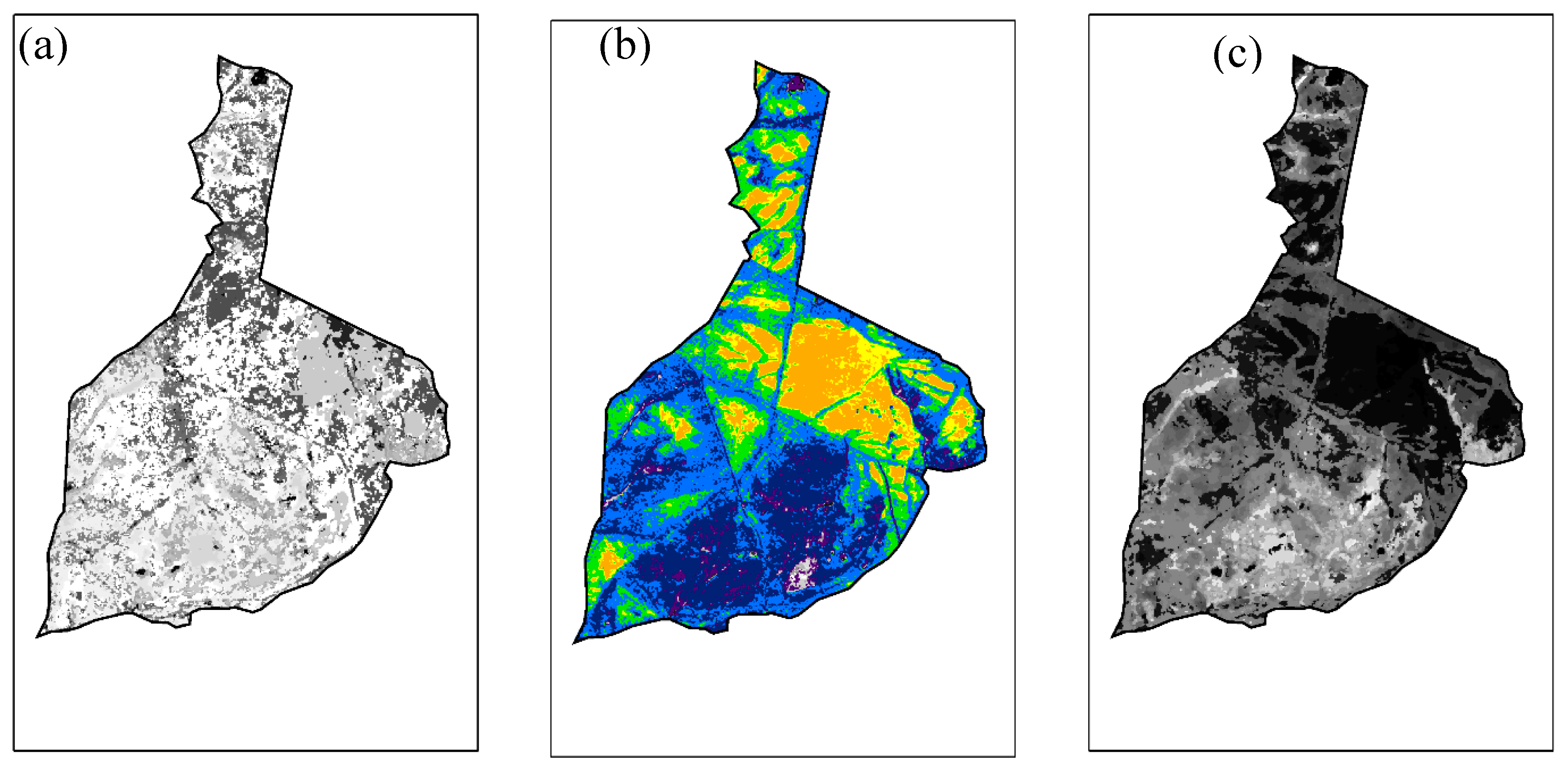
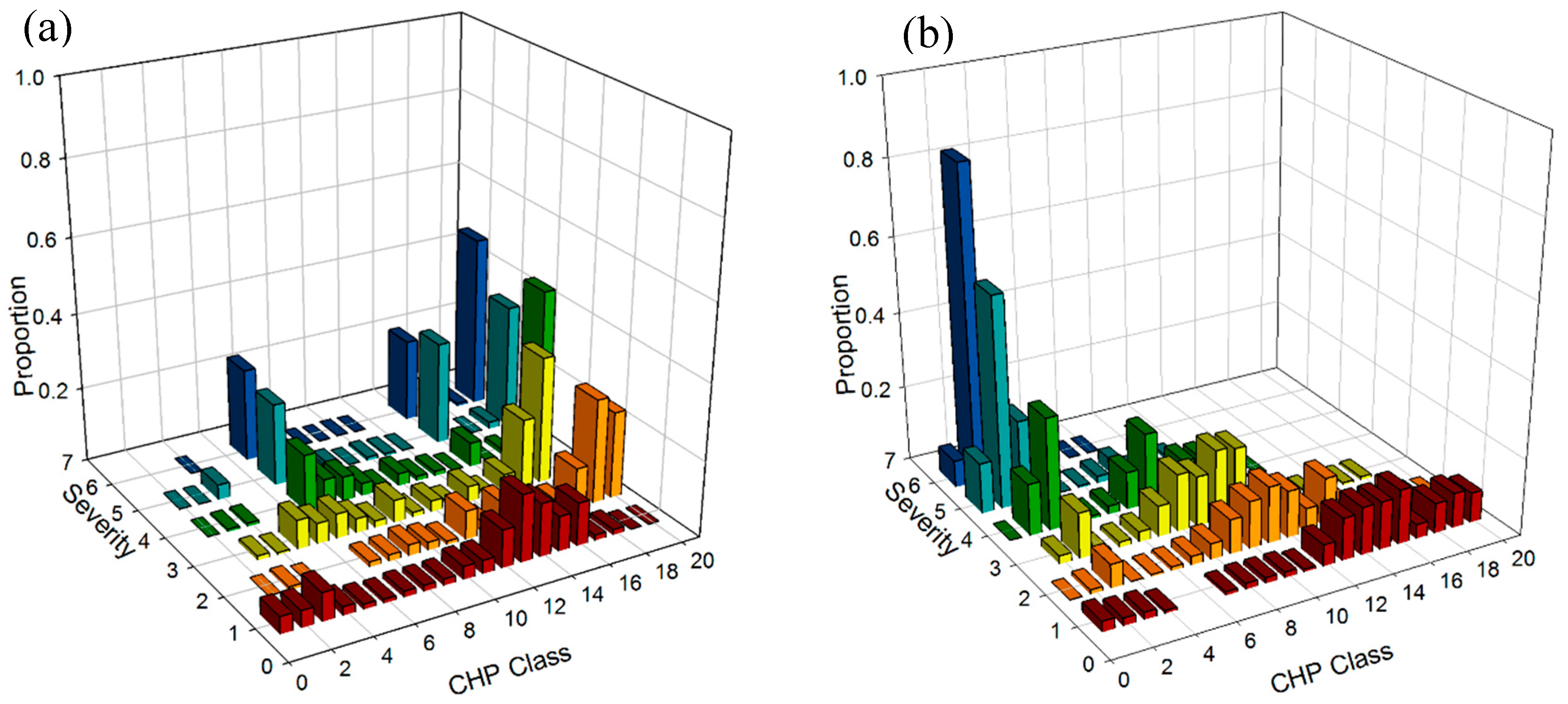
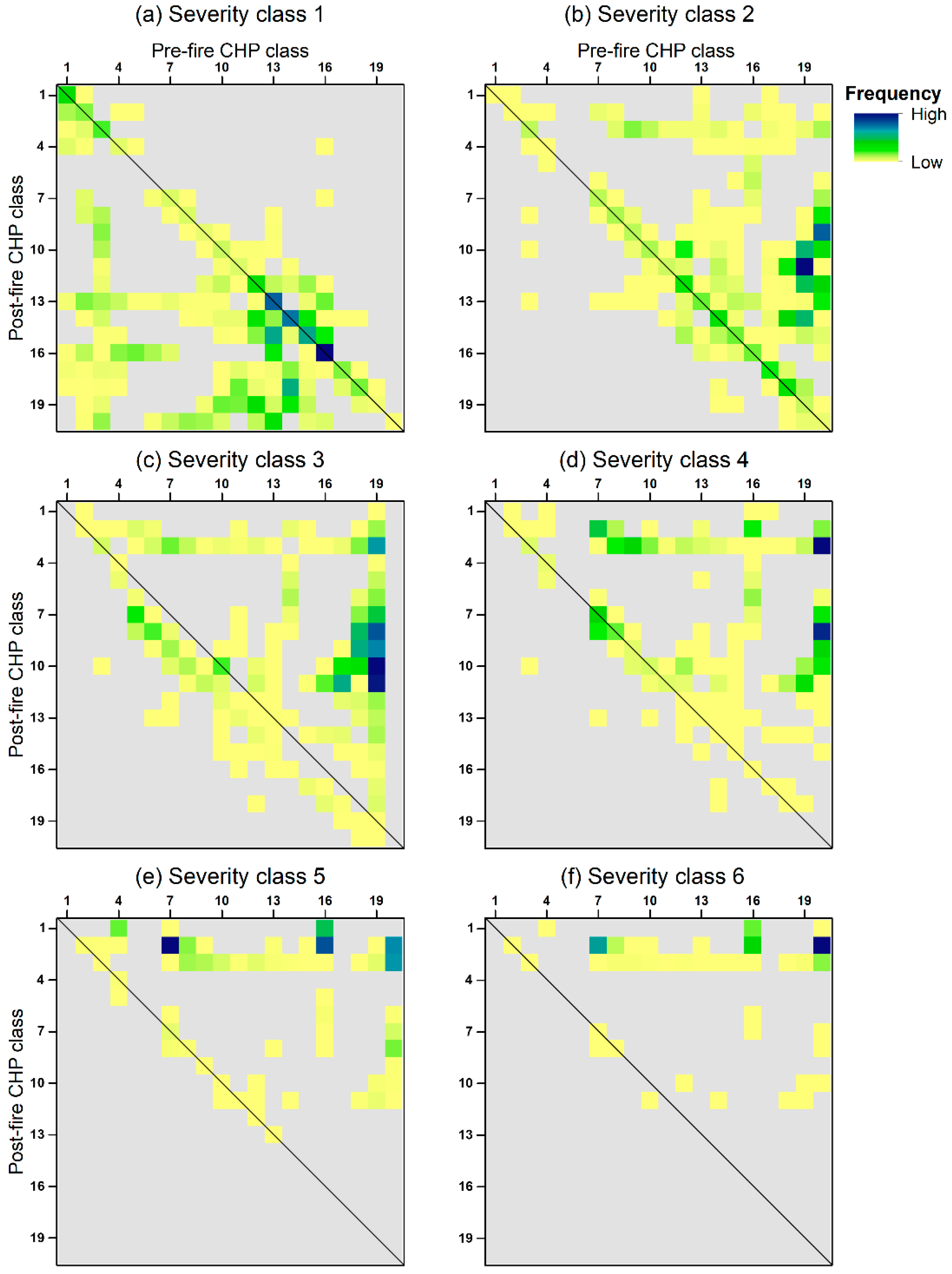
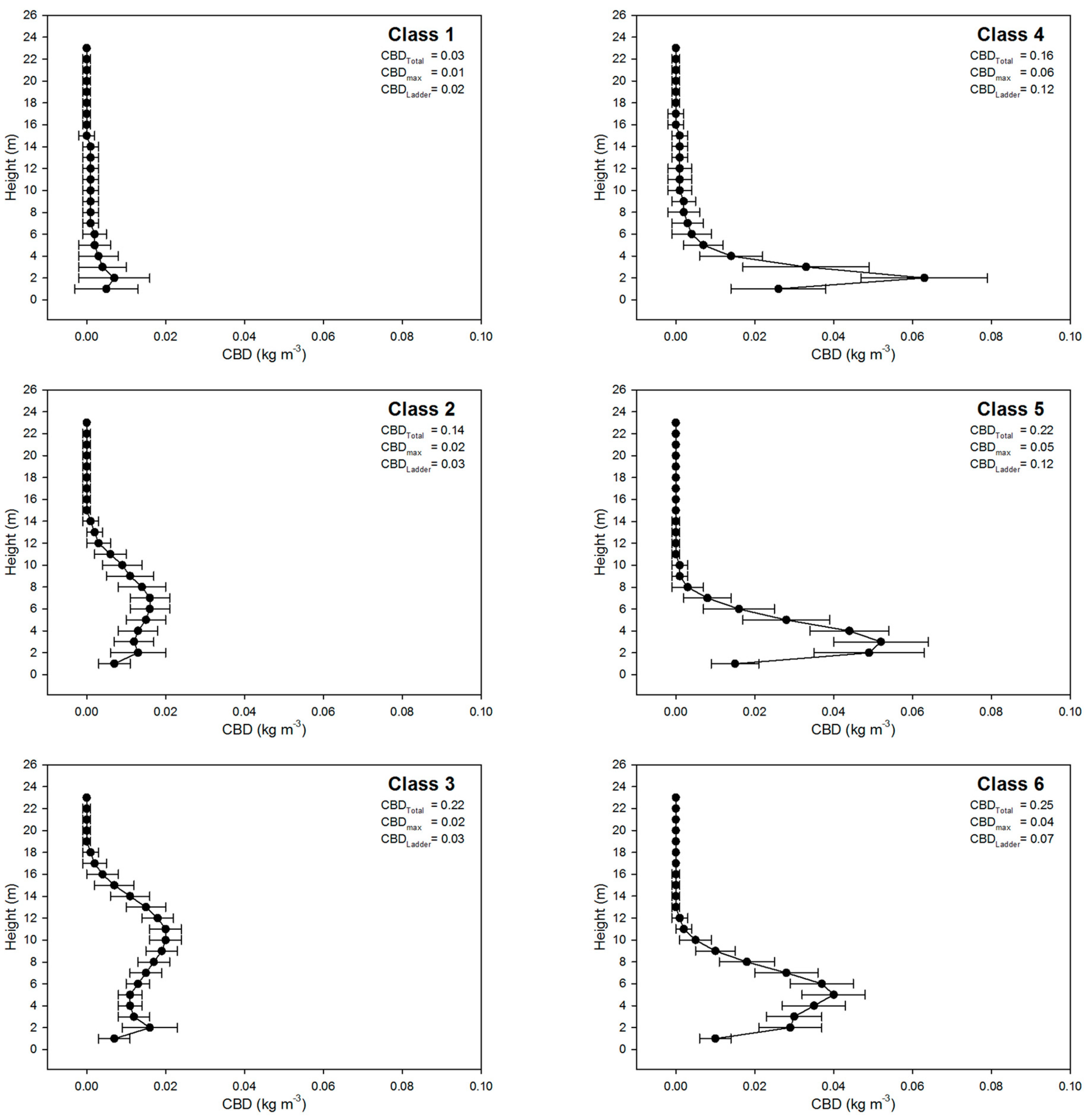
The objectives of this study were focused on examining the interaction between forest structure and fire severity using a time series of both active (ALS) and passive (WV-3) remote sensing datasets. To simplify the three-dimensionality of the canopy across the landscape, we used an ISODATA classification to derive categorical classes of canopy shapes, thus statistically separating the data and allowing for a two-dimensional analysis. Several classes dominated the landscape pre-fire, but transitioned to various new classes, depending on the severity of fire. Following the fires, the higher burn severity regions were dominated by classes with a larger CBDladder component and generally lower CBDmax position in the canopy (lower crowns). There were obvious patterns in the transitions between classes that were dependent on the severity of the fire, with mostly unchanged CHP shapes in the low severity classes, a wide diversity of transitions in the mid-severity classes, and transitions to a low diversity of post-CHP classes for the high severity pixels. The spatial patterning of the landscape changed relative to fire severity, with increasing fire severity resulting in larger patches and a lower diversity of canopy classes.
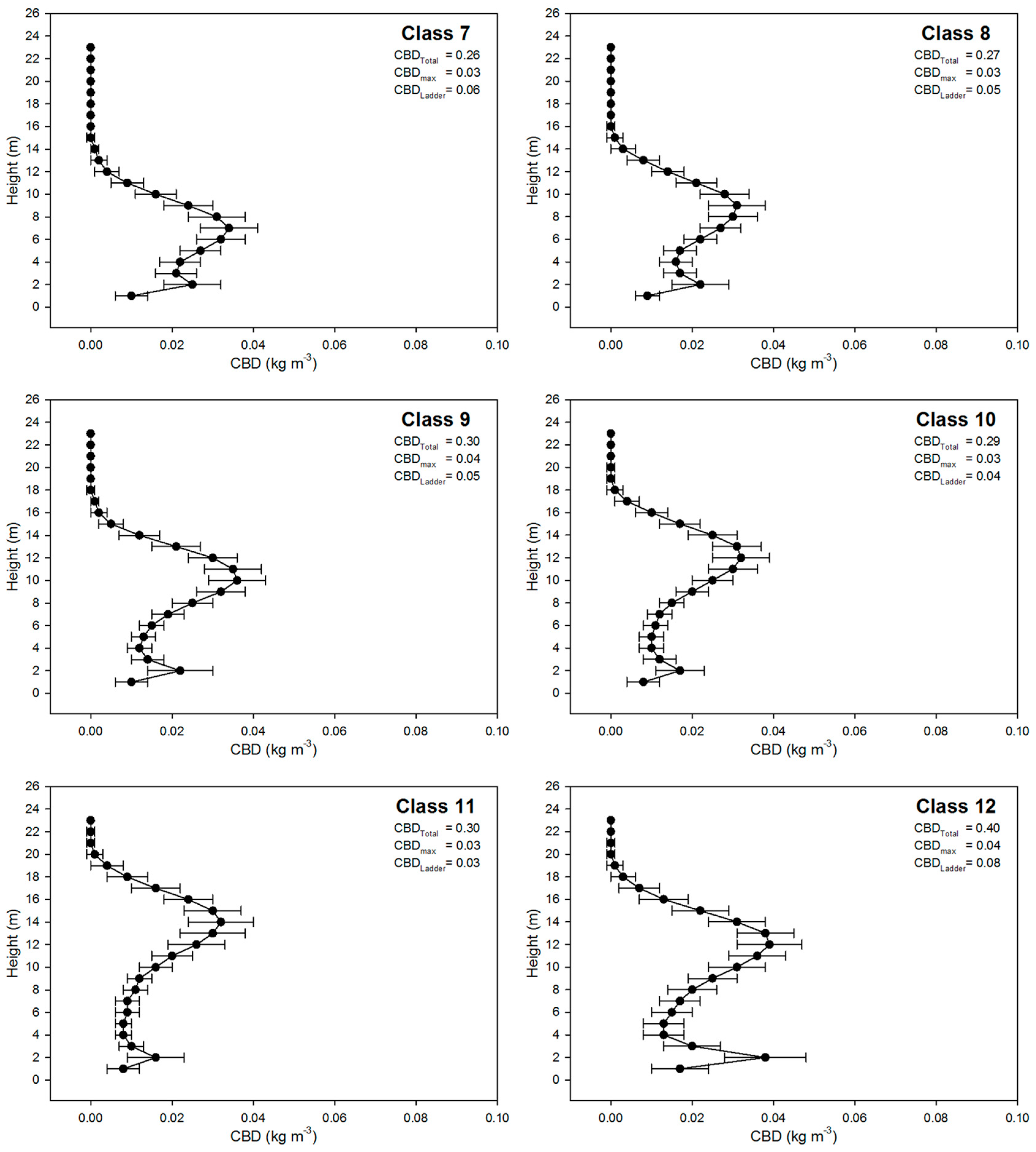
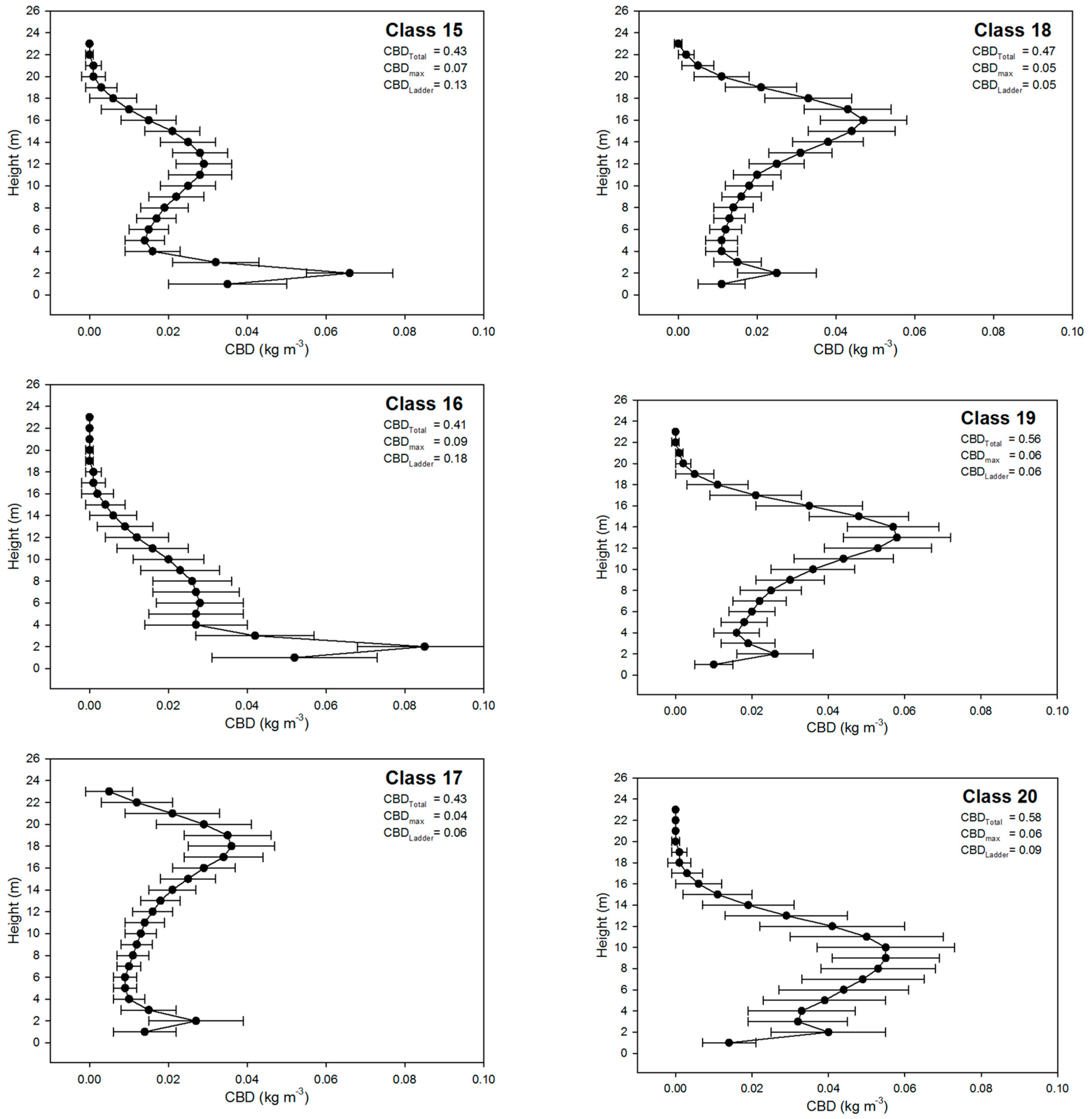
Using OLS-regression analysis, we were able to partition the effects of fuel loading, canopy shape, and firing pattern variables. We found that certain variables were distinctively more important than others in these regressions. CBDcanopy, CBDmid:CBDcanopy, CHP class 12, and heading fire ignition were relatively strong positive correlations in the model, while several CHP classes (2, 4, and 16) and backing fire ignition had the strongest negative correlations with fire severity. The results of the OLS analysis illustrate the importance of canopy fuel loading and canopy shape on fire severity. Surprisingly, most individual fuel loading variables that we considered did not have a strong influence. However, the strength of the CBDmid:CBDcanopy ratio in the model illustrates that the proportion of fuels in different canopy strata have a great influence on fire behavior. This result is interesting because it illustrates the need to understand where fuels are, not just the total amount or the maximum amount of fuels. This is further demonstrated in our analysis of CHP classes as a few of these classes had large relative importance, either positively or negatively influencing fire severity. Of the classes with the strongest negative influence, classes 4 and 16 are very similar in that they have very high fuel loads at the base of the canopy and very little overstory fuel. Because of the high density of the understory, it is possible that fuels may have been wetter and not as receptive to fire or that high drag due to the high fuel loads may have negatively influenced fire behavior. Conversely, CHP class 12 had a positive influence in the model and had a bi-modal distribution of fuels that were nearly equal in the canopy and mid-canopy strata. Our results indicate that the vertical distribution of fuel is an important factor and that subtle differences have defined effects on fire behavior.
Factors like topography, fuel moisture status, meteorological conditions, and ignition technique obviously have a strong influence on fire behavior and resulting severity. We chose to ignore topographical influences in this study because there is very little topographic variation in the area of interest, though we may have missed the effect of lowland areas in the study which would have had higher fuel moisture contents. Following Wimberly et al. [
46], we used the date of burn as a way to attempt to broadly account for meteorological and fuel status variation. However, likely because the burns happened over a short span of time, this variable did not increase the strength of the model and is therefore not reported here. Ignition pattern, as expected, had a very strong influence and greatly improved our prediction of fire severity. Not surprisingly, heading fire had a positive correlation and backing fire had a negative correlation on fire severity, while flanking fire did not have enough of an influence to enter the model.
The classification of ALS data into CHP profiles provides a way to simplify the representation of the vertical canopy structure, much the way that landcover is classified into representative groups using spectral reflectance datasets. Recently, Hoff et al. [
47] used a classification approach to classify the landscape using various ALS-derived variables and aligned these with Landsat-derived burn severity data [
48] for their area of interest. Using a classification scheme allowed us to group similar canopy profiles and to display them two dimensionally, thus allowing us to make use of more standard analysis techniques for two-dimensional datasets while still maintaining the ability to make inferences about the data in the context of vertical forest structure. Mutlu et al. [
49] made use of ALS data for the classification of fuels on a landscape into seven of the Anderson fuel models [
50]. While this work represented a step towards using ALS data as auxiliary data for developing maps of fuels for input into fire behavior models, such as FARSITE [
17], the technique did not explicitly account for vertical fuel structure or provide a way to directly examine physical changes in canopy structure. As fire modeling continues to move toward a CFD approach that integrates physical estimates of structure [
51], more detailed physical representations of forest canopy structure in three-dimensions are necessary. By representing forest structure using a classification scheme, our results allow for an examination of the transitions from pre-fire structure to the resulting post-fire structure. Looking closely at individual CHP class to class transitions is valuable because it could potentially allow prescribed fire managers to modify fire behavior with intentions of converting from one stand structure to another.
Our results indicate that varying levels of fire severity affect forest heterogeneity in much different ways. For instance, high severity fire has a much greater influence on Simpson’s Diversity Index than low intensity fire. Additionally, looking broadly at the transition matrices illustrates that diversity decreases not only in the arrangement of classes across the landscape with severity, but also affects the number of classes that appear following the fire. So, both horizontal and vertical diversity are inversely related to higher fire severities.
Our study also contributes to the debate regarding the limitations of spectral indices of burn severity, such as the WV-3 data we used [
19,
22,
23].
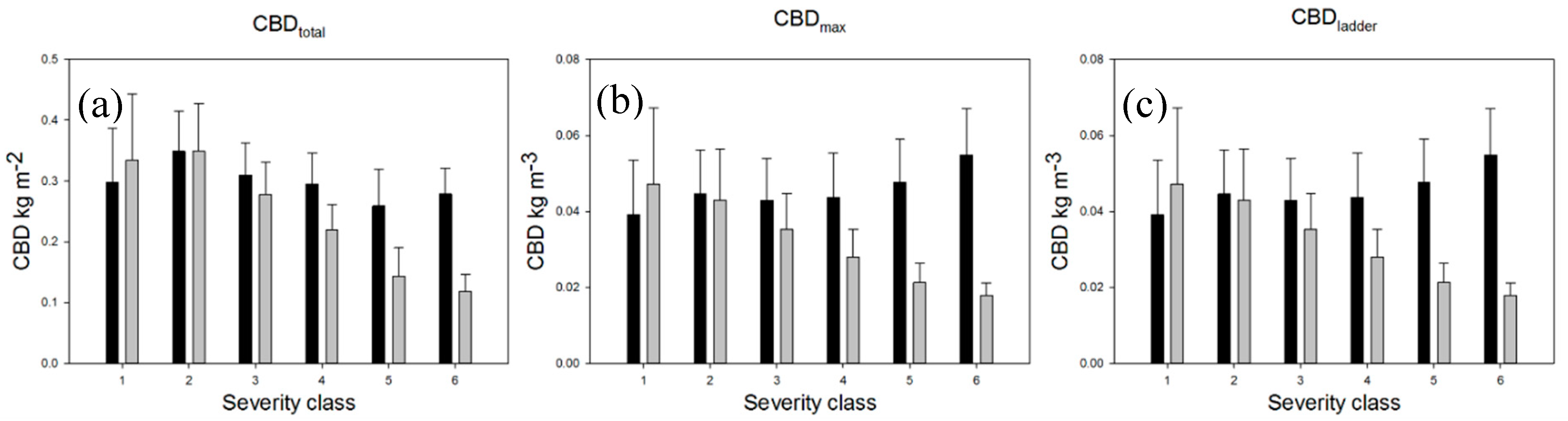
Figure 5 and
Figure 6 demonstrate that 2-D spectral indices are inherently limited, and that a spectral burn severity index value (such as our severity class 3) encompasses a wide range of structural changes to the forest. Indeed, any single measure of burn severity, even those derived from multi-temporal ALS data, such as the changes in CBD
total, CBD
max, and CBD
ladder shown in
Table 5, obscure distinctions in the changes and the resulting physical structure of the forest that may be important for resource managers and scientists alike. Therefore, we recommend that 3-D characterization of burn severity should be a major focus of future remote sensing fire research.
There are several limitations to this study. Field validation and verification is always challenging when considering forest structural characteristics that move beyond simple height or cover metrics. Because of the opportunistic nature of our study, we used previously developed models that estimated CBD for each bin [
52]. These models were developed from plot data within 10 miles of our site and in the same forest type, so they were deemed to be suitable. It is notable though, that allometric estimates of canopy bulk density profiles, which typically rely on diameter and height measurements of individual stems, would not be effective in estimating the canopy bulk density of stems that had been fully or partially consumed by fire, thus making our technique superior as it directly estimated these changes. Ideally, fuel plots would have been installed prior to the fires and allometry used to estimate canopy bulk density [
53], with models derived to estimate these variables to the ALS data [
54]. In this study, though we use models and method verification from published studies [
55], we are reliant on the ALS data to provide estimates of overstory consumption. There are also limitations directly associated with the parameters of the ALS data collections. Ideally, the ALS data would have been conducted immediately prior to and following the burn in order to best characterize the immediate impacts on the canopy. Additionally, there was likely some incongruity between the post-processed data products as flight altitude, sensor, sampling density, and other collection specifications were not identical. This is not a trivial issue for transfer of our methodologies to other regions because of the difficulty obtaining robust pre- and post-ALS surveys, especially in the context of a wildfire.
Further investigation of forest canopy structure, as it applies to wildland fire, is necessary in order to better provide the necessary inputs for CFD modeling, basic studies of heat transfer through fuel elements, and an understanding of combustion across landscapes. These studies of canopy structure are critical for improving our understanding of momentum fluxes through forest canopies and into and out of combustion zones. This work will also be important for the development of tools for pre-suppression planning for the mitigation of wildland fire, informing management objectives on the implementation of prescribed fire and for the evaluation of wildland effects and prescribed fire effectiveness. While ALS data has proven to be a good tool for landscape scale studies, these same CHP ideas may also transfer to both space-born LiDAR systems such as GEDI [
55] and small-scale TLS data collections [
56]. The power of these measurements and their application will be amplified as more spatially coincident collections are made which will allow for the examination of disturbance interactions and long-term trajectories across landscapes, as we now see coming to fruition with the Landsat data archive.
Our study aimed to develop our knowledge of the interactions between pre-fire fuel loading, fire severity, and post-fire fuel loading. We found that the pre-fire vertical distribution of fuels is an important factor in predicting fire severity across the landscape, most notably the ratio of mid-story to overstory fuels. Additionally, our classification approach demonstrated obvious patterns of transition CHP classes that were dependent on the severity of the fire, with mostly unchanged shapes in the low severity classes, a wide diversity of transitions in the mid-severity classes, and a low diversity of high frequency transitions for the high severity pixels. Finally, we found that the overall structural heterogeneity in our study area, both horizontally and vertically, was reduced in a way that was directly proportional to fire severity and resulted in a new set of conditions.


