
Spatiotemporal Prescribed Fire Patterns in Washington State, USA


School of Environmental and Forest Sciences, University of Washington, Seattle, WA 98195, USA
*
Author to whom correspondence should be addressed.
†
These authors contributed equally to this work.
Fire 2021, 4(2), 19; https://0-doi-org.brum.beds.ac.uk/10.3390/fire4020019
Submission received: 15 March 2021
/
Revised: 16 April 2021
/
Accepted: 20 April 2021
/
Published: 23 April 2021
(This article belongs to the Special Issue Wildfire Management in Increasing Complex Socio-Ecological Environments: Needs and Challenges)
Abstract
:We investigate the spatiotemporal patterns of prescribed fire and wildfire within Washington State, USA using records from the state’s Department of Natural Resources (DNR). Spatiotemporal comparisons of prescribed fire and wildfire area burned revealed that (1) fire activity broadly differed between the eastern and western portion of the state in terms of total area and distribution of burn sources, (2) over the 2004–2019 period, wildfire largely replaced prescribed fire as the predominant source of burning, and (3) wildfire and prescribed fire occur during distinct months of the year. Spatiotemporal variation in prescribed fire activity at regional levels were measured using five parameters: total area burned, total biomass burned, burn days, burn approval rates, and pile burn frequency. Within-region spatial variability in prescribed fire parameters across land ownership categories and bioclimatic categories were often detectable. Regression models of the annualized prescribed fire parameters suggested that prescribed fire activities have been declining in multiple administrative regions over the 2004–2019 period. A descriptive analysis of seasonal trends found that prescribed fire use largely peaked in the fall months, with minor peaks usually occurring in the spring. Lastly, we described how area burned, biomass burned, and pile burn frequency differed between prescribed fires approved and denied by the DNR, and found that approved prescribed fires were typically smaller and burned less biomass than denied fires.
Keywords:
prescribed fire; smoke; Washington; controlled burn; pile burning; environmental policy; permitting1. Introduction
Humans have deliberately burned landscapes across the globe for nearly a millennia to improve their surroundings [1]. For instance, indigenous people in the Pacific Northwest and elsewhere have historically used fire to clear land, hunt, and encourage economically beneficial plants [2,3]. With the arrival and expansion of European settlers starting in the 17th century, the North American populations of indigenous people were decimated and replaced with populations that were less tolerant of fire [3]. Indeed, reductions in fire frequency coincided with these demographic changes, which in turn altered the original ecology. Fire exclusion has resulted in hazardous accumulations of flammable fuel, loss of ecosystem services, and biodiversity loss in plant and animal species [3]. The numerous negative effects of fire exclusion eventually became apparent to land managers, and the purposeful use fire by humans to achieve ecological and land management objectives, hereafter prescribed fire, became an increasingly popular practice. In modern times, fire has not only found use in recreating historical ecosystem functions, but also in pest and disease control [4], disposal of logging slash [3,5], land clearing, game habitat improvement, and wildfire hazard mitigation [6].
Although the fire exclusion policies of the early half of the century have since relaxed, increases in prescribed fire application in the United States have mostly occurred in the Southeastern portions of the country [7]. At least part of what may be constraining prescribed fire application in other regions are negative public perceptions of prescribed fire [8]. Individuals with negative perceptions of prescribed fire are likely to emphasize the negative side effects of the practice. Despite generally producing less smoke than wildfires [9,10], prescribed fire smoke may still pose a health risk. Individuals with lung and cardiovascular disease, infants and unborn, and those from lower socioeconomic classes are particularly susceptible to negative smoke-related health outcomes [10]. Public safety can also be negatively impacted by prescribed fire smoke due to reductions in visibility for aircraft [11] and automobiles [12,13]. Although rare, prescribed fires have, on occasion, escaped to become wildfires, threatening human health and damaging property [7]. Prescribed fire smoke may also simply be a perceived nuisance to the public, who find it even more bothersome than equivalent quantities of wildfire smoke [14].
Most negative side effects of prescribed fire, unlike wildfires, can be lessened through specific burning practices. Smoke impacts in particular are mitigated through three general strategies: reducing the amount of area burned or fuel consumed, increasing combustion efficiency, or burning during conditions ideal for smoke dispersal away from populated areas. Of these three strategies, reducing the area burned or biomass is perhaps the most intuitive method of reducing emissions from prescribed fires [15]. Fuels that were planned to be removed through burning could instead be removed via mechanical treatments or grazing [6]. As discussed earlier, although the immediate smoke impacts may be reduced, fire exclusion can be costly in other ways [3], and managers may wish to lessen the emissions using methods that permit them to continue burning. Beyond reducing the amount of fuels to be burned, the amount of emissions produced from the fuels can be decreased by increasing combustion efficiency (i.e., the ratio of energy produced from fuels to the energy it contains) [16]. By increasing the amount of time in active flaming and limiting the amount of smoldering, the duration of the fire, and the amount of emissions, are reduced [10]. Combustion efficiency can be increased via a number of practices including pile burning, using backing fires, burning under low fuel moisture contents with low bulk density, rapid fire extinguishment following the prescribed fire, mass ignition, and supplying oxygen to the combustion process. In addition to using methods that reduce the volume of pollutants released from a prescribed fire, prescribed fire may be ignited in remote locations [16] or during times when atmospheric conditions dilute the pollutants before reaching human settlements [17].
Smoke mitigation practices can still sometimes conflict with other objectives or needs. Pile burning can damage soil biota [5], certain burning practices might encourage pests and disease [17], mechanical treatments may be economically expensive [18,19], and the meteorological conditions favorable for smoke dilution are less common than desired by land managers [20,21]. Consequently, minimizing smoke impacts might require incentivizing burning practices that might not otherwise be adopted because of these conflicts. One major incentive comes in the form of regulations, which can exist at the federal, state, and local level. At the US Federal level, the Clean Air Act sets air quality standards that all states are generally required to conform to [22]. Some states adopt even stricter standards than federal ones, which are outlined in smoke management plans. Occasionally, local nuisance emission standards also apply, further constraining prescribed fire application [16]. Smoke management plans and other policies often attempt to balance conflicts between maintaining high air quality standards, and the ecological and hazard reduction benefits of prescribed fire practices [23]. Although in the process of being revised, the smoke management plan in Washington State is particularly strict and has been identified by land managers as a barrier to prescribed fire use [24].
The Washington smoke management plan requires that all silvicultural burning over 100 tons be approved through the DNR. Burning permits are submitted by landowners, which are then approved or rejected based on multiple factors including current and forecasted air quality, current and forecasted meteorology, atmospheric conditions, and the availability of fire suppression resources [19]. These archived and publicly available administrative records, hereafter smoke management requests, provide detailed information regarding historic levels of prescribed fire use that cannot be revealed using data sources that only report area burned [7]. These administrative records may better represent prescribed fire activity than satellite data, which for multiple reasons might fail to detect prescribed fires [25]. Hence, these data are a valuable source of information for measuring variability in prescribed fire activities and identifying environmental correlates.
In this paper, we use administrative records from the DNR to investigate four questions about the spatiotemporal variation in prescribed fire activities in Washington State.
- How does prescribed fire area burned covary with wildfire area burned?
- How do prescribed fire activities covary with land ownership or vegetation?
- How do prescribed fire activities vary with time?
- How do prescribed fires that are approved by the DNR differ from those that are denied?
These four questions about spatiotemporal variation in prescribed fire activity can inform multiple land management and ecological objectives. For instance, resolving question 1 would gauge the relevance of prescribed fire and wildfire to variation in smoke, as smoke could be largely attributed to prescribed fire in one setting and wildfire in another. Given prescribed fires use as a wildfire hazard mitigation tool, it is also valuable to measure the magnitude of the correlation between prescribed fire and wildfire area burned. Prescribed fire’s utility as a land management tool also means the spatiotemporal variability in its use can be informative to decisionmakers who want to understand where future applications are needed or gauge the effectiveness of historical prescribed fire policies and strategies. To that end, question 2 will help us understand where, within administrative regions, prescribed fire activity is high and where it is low, and determine to what extent this spatial variability can be attributed to differences in ownership or bioclimatic variables. Understanding when prescribed fire activities differ can be as important as understanding where they differ. For example, knowing when prescribed fire is likely to be high will inform of times when air quality might be negatively impacted, which can help public health professionals effectively mitigate the associated health impacts. Our investigation of question 3 will describe how prescribed fire activities have changed over time, both over long time scales and over the course of a year. Land managers would prefer that burn requests they submit are granted. Our investigation of question 4 advances that end by describing what conditions coincided with prescribed fire approvals and denials, which is information that can be used by land managers to develop more effective burn strategies, and predict when prescribed fires are likely to be approved.
2. Methods
2.1. Data
Smoke management requests were provided by the DNR for the years 2000–2019. Each row in the data corresponds to an individual burn request and the columns include information such as the latitude, longitude, burn category (Broadcast, Natural, and Pile), ignition date, proposed acres, proposed tons, accomplished acres, and accomplished tons. Proposed large prescribed fires (>100 tons) in Washington State are conditional on approval at a division and region level [19], and two additional data columns indicate whether approval at both levels was granted. We classified a prescribed fire as approved if an explicit yes decision was given from both. We note here that if approval is given by one level, it is nearly always given by the other (Pr () ≈ 0.99997 and Pr ( 0.97514). Burn categories were defined as follows: requests to burn slash left on the ground were classified as broadcast, requests to burn the landscape in the absence of any pre-burn mechanical treatments were classified as natural, requests to burn slash that is piled into one location were classified as pile. These categories were further simplified into binary pile and non-pile burns. Data from 2000–2003 were omitted due to observed inconsistencies compared to the rest of years (Figure S1). For the years 2000–2003, proposed and accomplished acres were in perfect agreement, proposed burn volumes were higher than accomplished, and every burn request was approved.
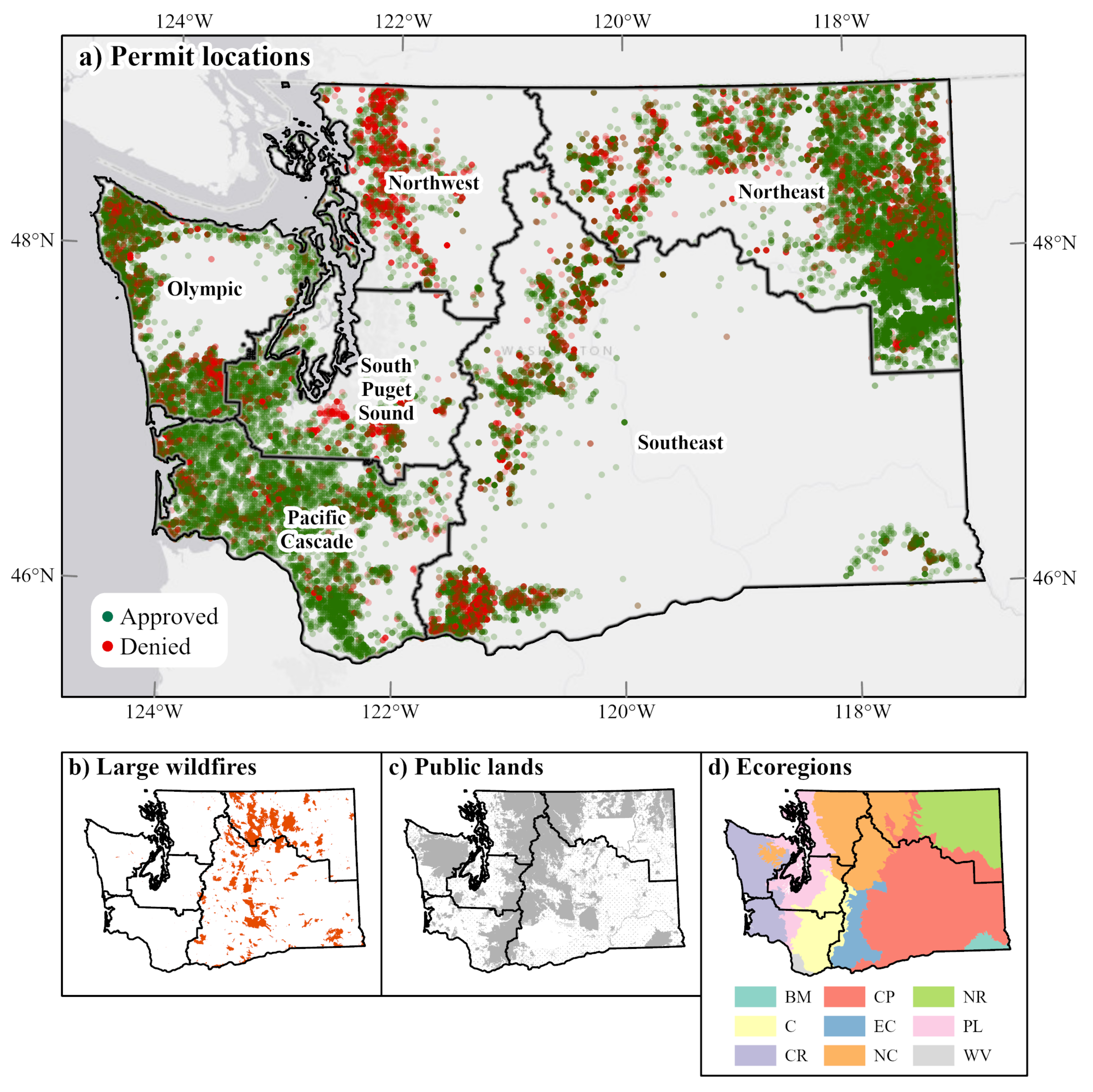
The coordinates of the 2004–2019 prescribed fires were mapped onto three spatial datasets: DNR administrative region boundaries (https://data-wadnr.opendata.arcgis.com, verified 4 April 2021), public land ownership boundaries (https://data-wadnr.opendata.arcgis.com, verified 4 April 2021), and EPA level III ecoregion boundaries (https://www.epa.gov, verified 4 April 2021). The administrative regions could describe how prescribed fire activity varied between six regions that are used for DNR decisionmaking (Figure 1a). Within administrative regions, the public-private ownership (Figure 1c) could describe differences in prescribed fire parameters under different management paradigms, and the ecoregion boundaries (Figure 1d) could describe how prescribed fire varied across different bioclimatic regimes. Private ownership was assumed to be any area that was not included in the public lands ownership boundaries. The number of fires in each administrative region, disaggregated by burn category and approval, is shown in (Table 1). The area and proportion of land within each administrative region split up by landownership category and ecoregion category is shown in (Table 2). In addition to DNR smoke management requests and other spatial data, wildfire area burned data from the DNR (https://data-wadnr.opendata.arcgis.com, verified 4 April 2021) were used to contextualize the spatial, interannnual, and seasonal trends in prescribed fire area burned (Figure 1b).
Prescribed fire activity was characterized using five parameters: total area burned, number of unique burning days, biomass burned, probability a burn request is approved, and the probability of a pile burn. A lack of follow up data regarding accomplished area and accomplished volume variables led us to analyze the proposed area and proposed volume burned instead. The potential influences of using accomplished rather than proposed burning were explored for each region by calculating the ratio of proposed and accomplished quantities where data were available. Analysis of this ratio revealed that (1) it was often near one suggesting that the accomplished area burned was usually close to proposed area burned and (2) did not strongly vary in time. Further details are available in the Supplementary Materials. Add-one smoothing [26] was used to estimate approval probabilities and pile burn probabilities, the purpose of which was to differentiate between times when no burn requests are made versus when burn requests are made but denied. Without add-one smoothing, both cases would have approval probabilities of zero.
2.2. Statistical Analyses
2.2.1. Wildfire and Prescribed Fire
Spatial, interannual, and seasonal descriptions of area burned were produced for wildfires and prescribed fires. Spatial variability was described by comparing the average annual area burned of approved prescribed fires and wildfires for each administrative region. Interannual variability was described by modeling the annual area burned time series for 2004–2019 of prescribed fires and wildfires with linear regressions. Annual area burned was the response variable and year was the predictor. Interannual trends over the 2004–2019 period were identified by testing whether the slope of the regressions were significantly different from zero. Boxcox data transformations [27] were used to identify potential nonlinearities in the models. Whichever of the inverse (), log (), square-root (), identity (), or square () data transformations were closest to the the maximum likelihood estimate from the boxcox transformation was used as a potentially nonlinear alternative to linear regressions. The relative performance of the linear and nonlinear regression models was compared using the unadjusted values. Seasonal trends of wildfire area burned and prescribed fire area burned were calculated by finding the 10th, 50th, and 90th percentiles for each month using relevant data from 2004 to 2019. We tested whether a relationship was detectable in the two time series by estimating the Kendall correlation. We tested whether there was sufficient evidence to reject the null hypothesis that the monthly prescribed fire area and wildfire area burned time series were independent. Kendall correlations and significance levels were calculated using the “Kendall” package [28] with the default settings in the R programming language [29]. For this and all statistical tests, significance levels were analyzed using methods described by [30], which converted p-values into Bayes factors [31,32] which were interpreted through published rules-of-thumb regarding evidence strength [33].
2.2.2. Spatial Variation
For each administrative region, the difference between the annual averages of the five prescribed fire parameters were compared across land ownership categories (Figure 1c) and ecoregion categories (Figure 1d). The significance of differences between binary private–public categories was assessed using two-sided t-tests, which assume that the mean of the distribution of prescribed fire parameters of private and public lands are equal under the null hypothesis. The significance of differences between ecoregion categories were assessed similarly, but using a one-factor anova. Here the null hypothesis assumes that the mean of the distribution of prescribed fire parameters are equal in all ecoregions.
2.2.3. Temporal Variation
The monthly time series of each of the prescribed fire parameters was decomposed into interannual and seasonal components. Interannual trends were described by annualizing each of the five prescribed fire parameters for each year between 2004 and 2019 and using least-squares regression to summarize the data. Seasonal trends were described by calculating the average 12-month seasonal time series for each of the five prescribed fire parameters using 2004–2019 data. This 12-month seasonal time series component, or seasonal profile, was used to identify the major and minor modes of prescribed fire activity (i.e., when prescribed fires tended to peak each year). The major mode of the seasonal profiles was defined as all the local maxima of the seasonal profile equal to the largest values. The minor mode was defined as all the local maxima equal to the second highest value. Interannual variability in the modal month was calculated by estimating the probability that a month had the year’s highest prescribed fire activity as measured with the five prescribed fire parameters. As in the wildfire and prescribed fire analyses, interannual trends over the 2004–2019 period were identified by testing whether the slope of the regressions were significantly different from zero. Potential nonlinearities in the interannual trends were identified using the same boxcox analysis of Section 2.2.1.
2.2.4. Variation between Approved and Denied Requests
The difference in area burned, biomass burned, and burn type were compared across approved and denied burns. The significance of differences between area burned and biomass burned was assessed using two-sided t-tests. The significance of dependencies between burn approvals and burn categories were calculated using 100,000 Monte Carlo samples of a Chi-squared test [34]. All calculations were performed in the R programming language [29].
3. Results
3.1. Wildfire and Prescribed Fire
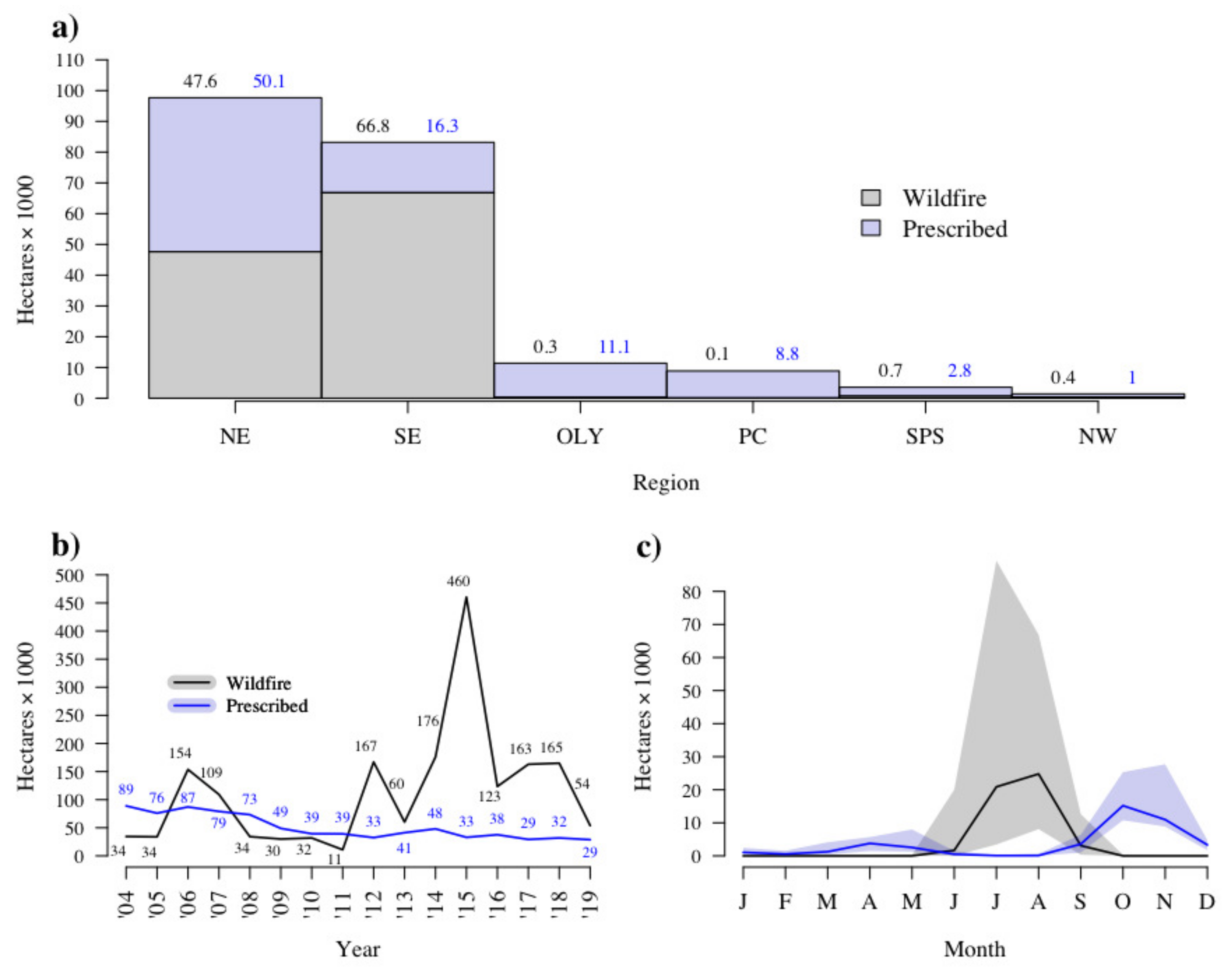
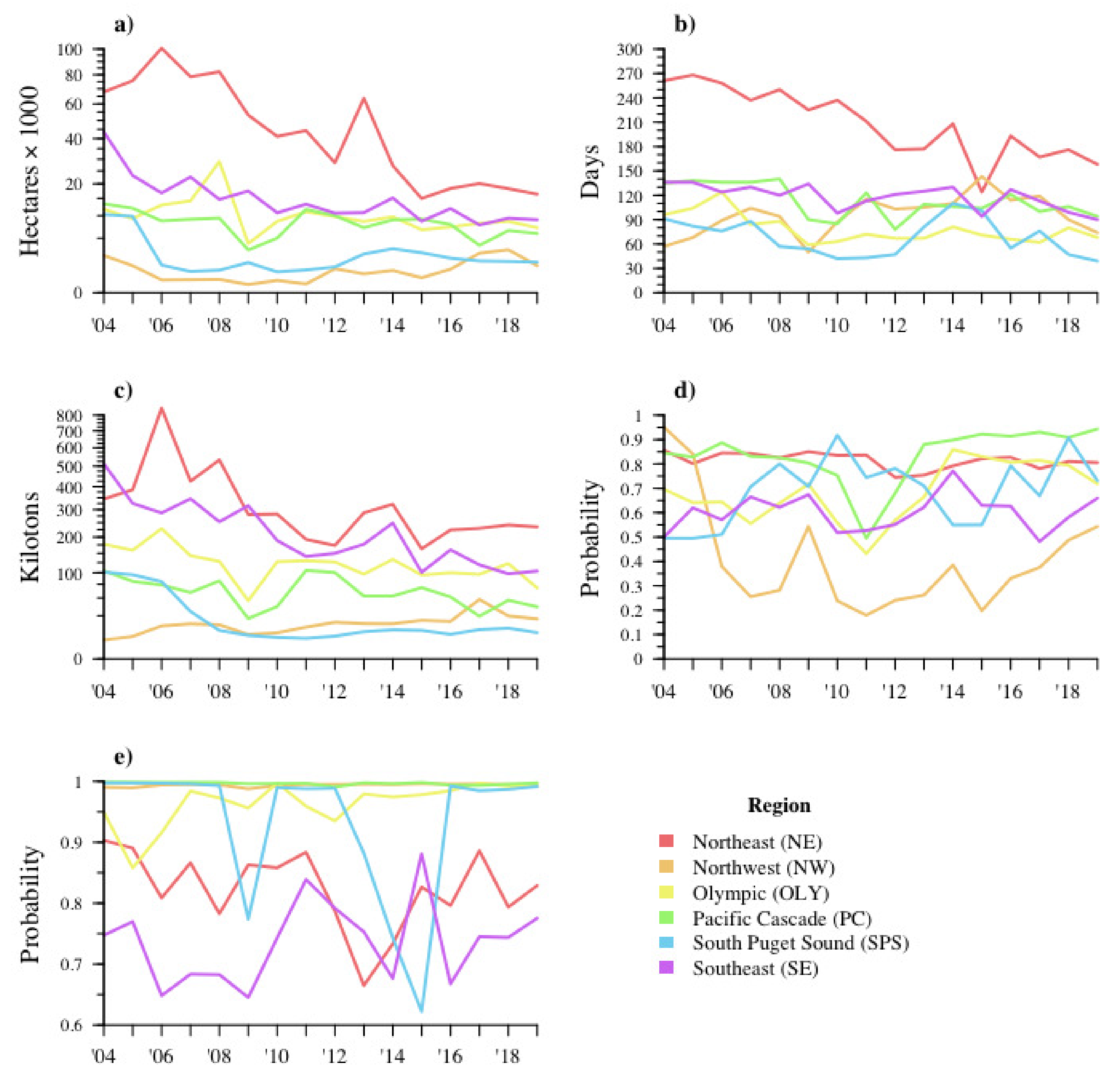
Approximately 116,000 ha were burned by wildfire, and 90,000 ha were burned by prescribed fire annually in Washington between 2004 and 2019. Wildfire and prescribed fire patterns differed between the eastern (SE and NE) and western (OLY, PC, SPS, and NW) portions of Washington. Large annual area burned rates (>80,000 hectares/year) commonly from (49–80 percent) wildfire are characteristics of eastern Washington burn patterns. In contrast, very little area burned in the western portions of Washington State, and most of that area was attributable to prescribed fires. The largest annual area burned in western Washington was observed in OLY, which burned approximately 11,000 ha each year, with 98 percent of this area attributable to prescribed fire. In other western regions, area burned ranged from 1400 ha/year (NW) to 8900 ha/year (PC), and the percent of area attributable to prescribed fire ranged from 74 (NW) to 99 (PC) percent (Figure 2a).
Over 2004–2019, the annual area burned by prescribed fire over Washington State decreased at a statistically significant rate of −4076 ha/year. In 2004, 89,000 ha of land were burned by prescribed fire, falling to 29,000 ha by 2019. Over this same time, the annual area burned by wildfire had a positive (+9084 ha/year), but insignificant trend. In 2004, 34,000 ha were burned by wildfire, and in 2019, this quantity rose to 54,000 ha. For prescribed fires, the raw annual area burned measurements were fairly well-described by a linear relationship (, but applying an inverse data-transformation did further improve the fit (. For wildfires, although the raw annual area burned measurements did not show a strong linear relationship with year (. Applying a log data-transformation did not improve the fit () nor did it reveal any detectable trends (Figure 2b). The nonlinear regression describing annual prescribed fire area burned suggest that over the 2004–2019 period the burn rate has decelerated. We also note that for many years before 2012, prescribed fire area burned was larger than wildfire area burned, but this was not observed after 2012 (Figure 2b).
Monthly area burned time series from wildfire and prescribed fire were estimated to have a very-strongly significant negative correlation ( = −0.40) (Figure 2c). In July–August, the median wildfire total area burned is typically its highest (21,000–25,000 ha) and prescribed fire area burned was very small (80–100 ha). In the remaining months, wildfire area burned was much lower, with a reported median area burned of zero October–May. Prescribed fire area burned was also much higher, peaking in October–November (11,000–15,000 ha) (Figure 2c).
3.2. Spatial Variation
3.2.1. Land Ownership
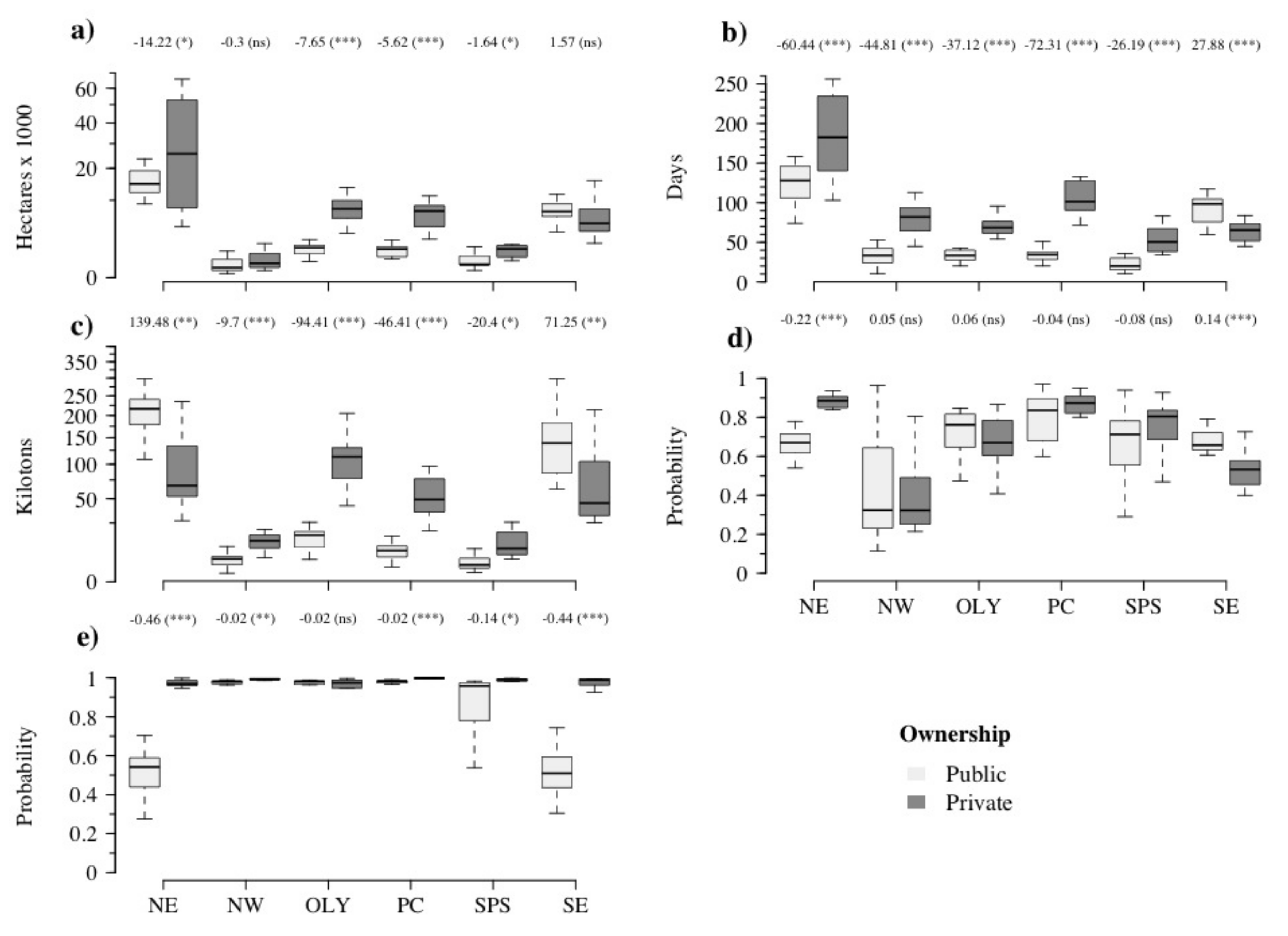
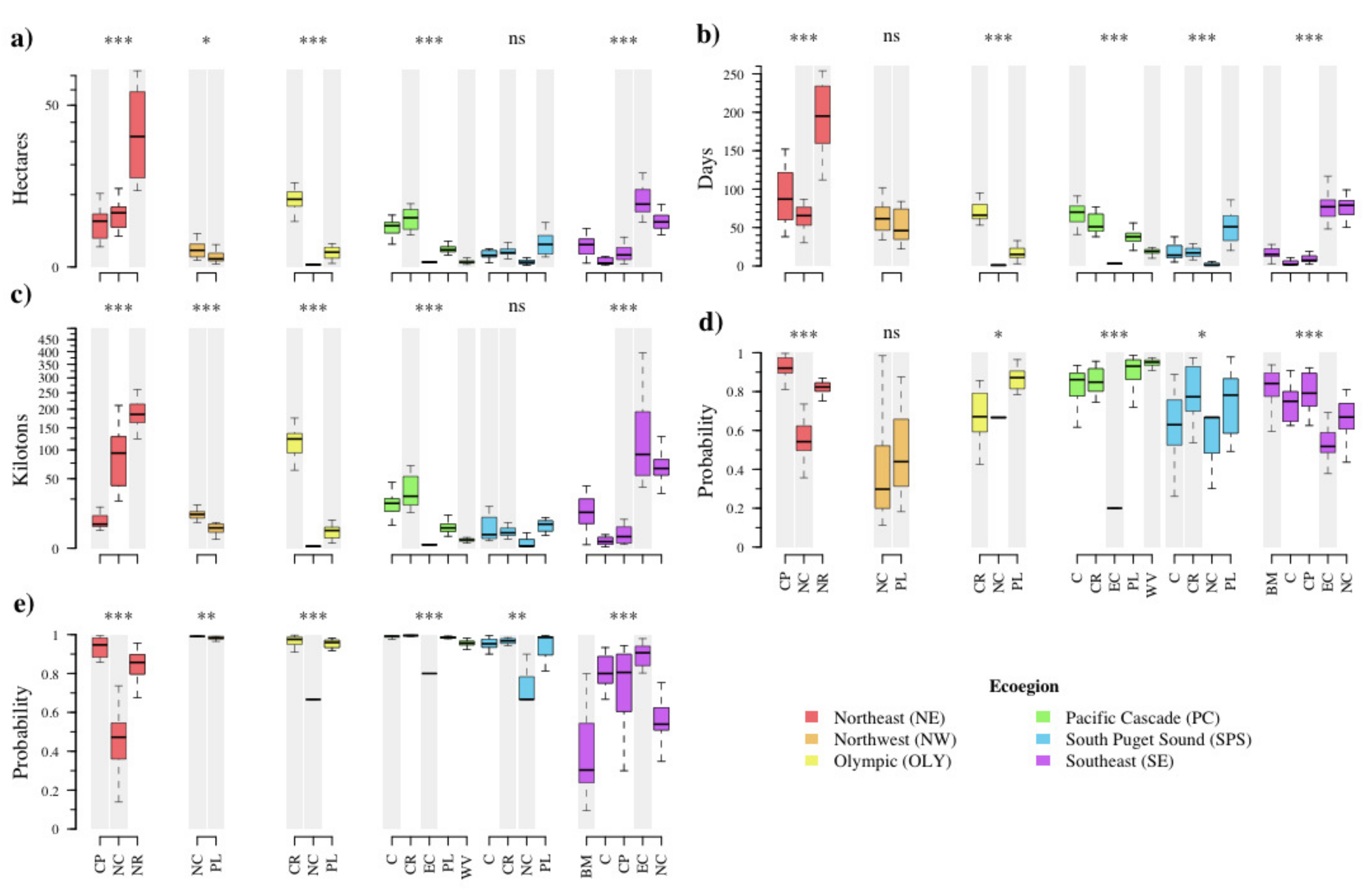
Detectable differences (i.e., unlikely to have occurred by chance) in the distribution of prescribed fire parameters between public–private lands were common. This trend was most consistently observed for the proposed burn days parameter, where in all six administrative regions, strongly-significant differences were observed. In all but the SE region, the number of unique days when prescribed fire was proposed was higher in the private lands than in the public lands. Although detectable differences were common for most prescribed fire parameters, approval probabilities were one exception. In all of western Washington (NW, OLY, PC, and SPS), the differences in the distributions between the approval probabilities on private lands and on public lands were not significant. In eastern Washington detectable differences were observed, but the effects of land ownership on approval probabilities were not the same in the NE and SE. In the NE, prescribed fires on private lands were more likely to be approved than prescribed fires on public lands, whereas in the SE prescribed fires on private lands were less likely to be approved than prescribed fires on public lands (Figure 3).
3.2.2. Ecoregions
The distribution of the five prescribed fire parameters commonly differed within each administrative region across a bioclimatic gradient. In other words, the mean prescribed fire parameters in one ecoregion were often noticeably different from one another. Exceptions were seen only in the SPS and NW administrative regions. In the SPS, there was insufficient evidence to conclude that the distributions of area burned or biomass differed depending on the ecoregion in which the burn was planned. In the NW, there was insufficient evidence to conclude that the distributions of burn days or approval probabilities differed depending on the ecoregion in which the burn was planned (Figure 4).
3.3. Temporal Variation
3.3.1. Interannual
Prescribed fire activity decreased from 2004 to 2019, but there was variability in the magnitude of this decrease across regions and prescribed fire parameters (Figure 5). Detectable changes in area burned ranged from −1395 hectares per year in the SE to −5142 hectares per year in the NE. Detectable changes in the annual number of burn days ranged from −2.11 days per year in the SE to −7.80 days per year in the NE. Detectable changes in biomass burned ranged from +1.43 kilotons per year in the NW to −21.3 kilotons per year in the NE. Few changes in approval probabilities and pile probabilities were detectable. Indeed no detectable changes in approval rates were observed in any of the regions, and a detectable increase was observed only in the NW and OLY (+0.0003 per year and +0.0049 per year, respectively) (Table 3).
3.3.2. Seasonal
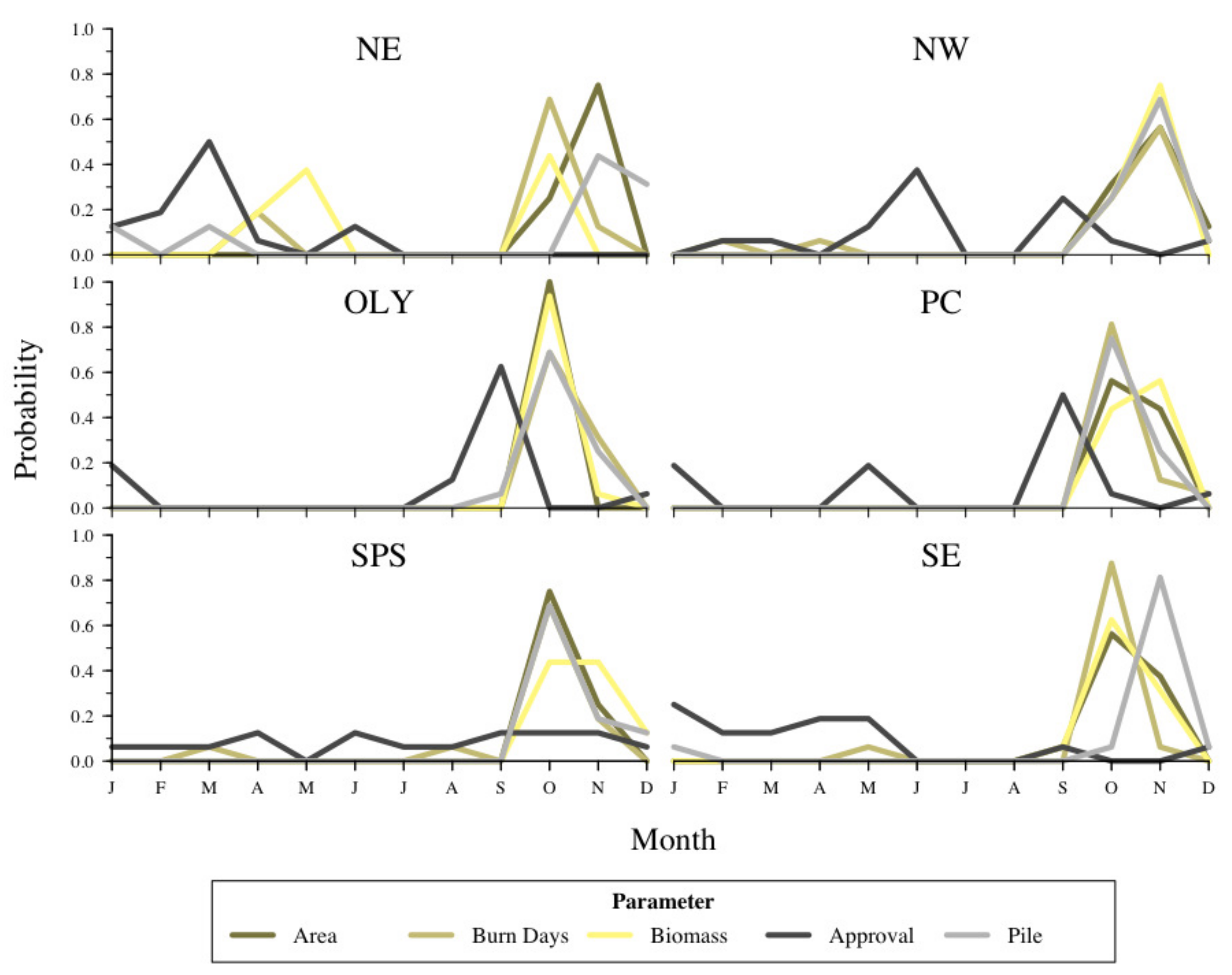
In most combinations of regions and prescribed fire parameters, prescribed fire activity tended to follow a bimodal seasonal profile, with the major modes occurring in the fall and minor modes in the spring (Figure 6). Area burned, burn days, and biomass burned peaked in the fall months in every region except the NE, where the expected area burned was highest in May. Although common, the usual seasonal pattern—bimodal with a major mode in fall and a minor mode in spring—was not seen in every pair of prescribed fire parameters and regions. Burn approvals were sometimes highest in the spring months, and half of the regions peaked in February, April, and May. In the NE and OLY, burn approval rates were highest in the summer (August), but the minor modes were similar in magnitude and occurred in spring months (Mar–Feb). In the NW as well, approval rates are also noticeably higher in the summer months compared to the shoulder seasons (Figure 6). Similarly, pile burn probabilities were highest between November and February. The typical bimodal seasonal profile was also unimodal in some cases. For instance, in the NW region, area burned and biomass burned peaked in November, with no other minor peaks. In the SPS, biomass burned also peaked in November only (Table 4). For any particular year, the peak of prescribed fire use did not always coincide with the major mode of the seasonal profile. In the NE for instance, although the expected burned biomass was highest in May, in most years the highest burned biomass occurred in October. In some years, as seen with burn days in the SPS, the peak of prescribed fire activity did not occur in the spring or fall (Figure 7).
3.4. Variation between Approved and Denied Fires
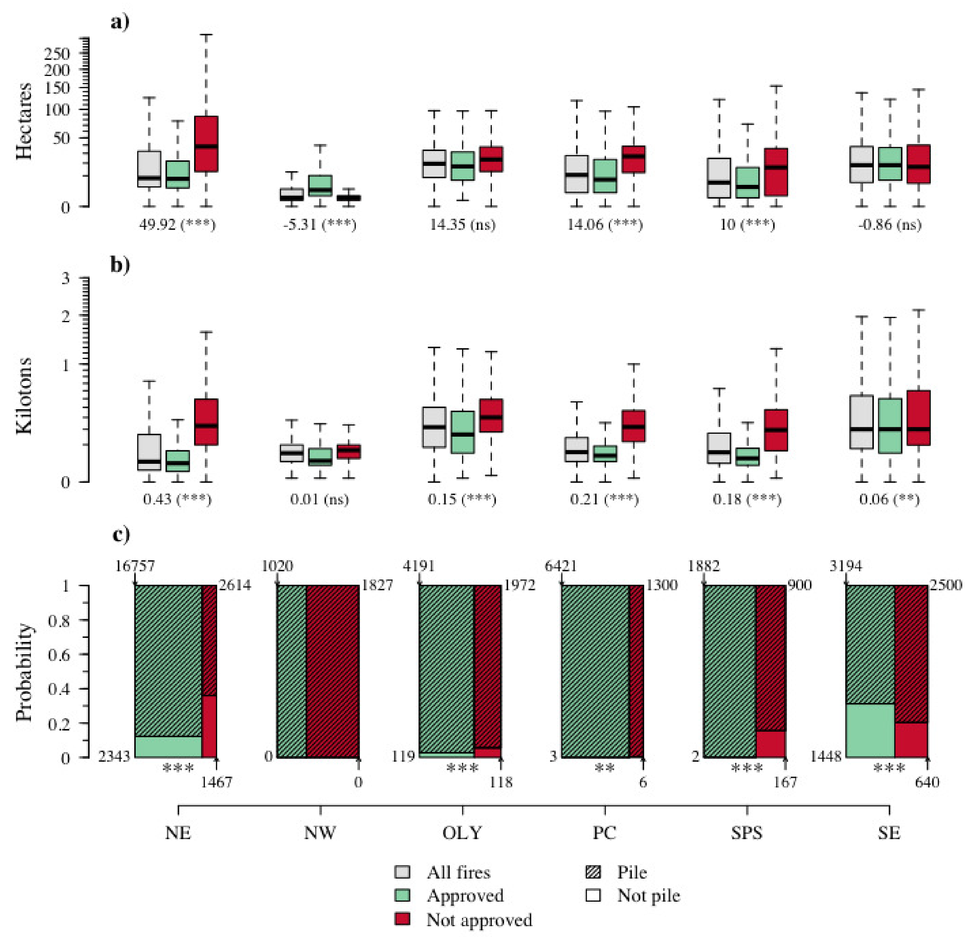
Approval rates were fairly spatially variable, ranging from 36 percent in the NW to 83 percent in the PC (Table 1). In most cases, the distribution of proposed burn characteristics differed between approved and denied burns. For instance, in the NE, NW, PC, and SPS the proposed area burned was significantly different in the denied burns than in the approved burns. In all but one of these regions (NW), the area burned was larger or similar the denied burns than in the approved ones. Similarly, in all regions except the NW, the proposed volume of biomass burned was significantly larger in the denied burns than in the approved burns (Figure 8). In addition to burning more area and more biomass, denied burns tended to be pile burns at frequencies that were significantly different from approved fires. In fact, for all regions except the NW, detectable dependencies were observed between approvals and burn categories. Unlike with area burned and biomass burned, the differences between approved burns and denied burns were not consistent across regions. In the SPS for instance, pile burns were proposed less frequently in denied burns than approved ones, but in the SE, this dependency is flipped so that pile burns were proposed more frequently in denied burns than approved ones (Figure 8).
4. Discussion
4.1. Wildfire and Prescribed Fire
Spatial and temporal patterns of wildfire activity can provide relevant contextual information about the relative impacts of prescribed fire. For instance, we found that in the eastern regions of Washington, prescribed fire and wildfire area burned were higher than in the western regions, suggesting greater impacts from smoke. Although the amount of area burned by prescribed fire in eastern Washington was higher, much of the total area burned in eastern Washington’s was still attributable to wildfire (Figure 2a). If provided with an estimate of the reduction in wildfire area per unit increase in prescribed fire area (the leverage) [10], land managers could determine the cost-benefits of increasing prescribed fire activity. Increasing the area burned by prescribed fire may increase smoke, but because wildfire smoke is especially unpredictable and hazardous, the increases in prescribed fire smoke may be offset by the reductions in wildfire area burned [9,10].
We also saw that, prior to 2012, the area burned by wildfire was often less than the area burned by prescribed fires. In fact, the area burned by wildfire has been larger than that due to prescribed fire ever since (Figure 2b). Some explanations for this trend are explored in Section 4.3.1. Additionally, we found that as monthly wildfire area burned increased in the summer, prescribed fire area burned decreased (Figure 2c). The implications of this correlation are explored in Section 4.3.2.
4.2. Spatial Variation
4.2.1. Land Ownership
Prescribed fire activities frequently varied across land ownership categories, which suggests that differences in land management strategies and constraints might explain part of the variability in prescribed fire parameters. For instance, the number of days of proposed prescribed fire was higher in private lands than in public. Although private lands are more prevalent in some administrative regions (Table 2), private lands still planned more burns in regions where this was not true. One explanation for this pattern is that burning on public lands are likely to be subject to more constraints than burning on private lands. For instance, prescribed fire on public lands may be concerned about smoke reducing visibility in locations valued for there scenic beauty [35]. Public lands could also be constrained through precautions or policies intended to protect vulnerable wildlife, which may not be required on private lands [36]. Hence, these additional considerations taken on by public landowners would result in burning less frequently relative to private landowners who were not subject to the same rules. On the other hand, it is often private land owners who perceive to have more legal and social barriers when planning prescribed fires than decision-makers on public lands [37].
4.2.2. Ecoregions
Prescribed fire activities frequently varied across bioclimatic regions, which suggests that local variation in vegetation and climate can impact prescribed fire activities. Patterns of wildfire burning are known to be influenced by bioclimatic conditions. One portion of the Cascades might have a mean fire return interval of 1000 years, whereas an area nearby may have fire return more than 10 times as frequent. Fire attributes, such as size and severity, can have meaningful levels of variation over fairly small spatial scales [38]. Hence, when prescribed fires are used as a surrogate for wildfire, prescribed fires might then vary spatially in patterns similar to wildfire. Differences in fuel load, flammability, and confounding of anthropogenic variables explain spatial variability in prescribed fire parameters within administrative regions. Forested ecoregions have relatively high fuel loads and therefore higher burned biomass than nonforested ecoregions (e.g., Columbia Plateau and Northern Rockies in NE). Nonforested ecoregions may also encounter conditions when fires may become uncontrollable more frequently, and therefore burn less frequently, than forested ecoregions (e.g., Columbia Plateau and East Cascades in SE). Additionally, lowland ecoregions may happen to have more human inhabitants resulting in different prescribed fire characteristics (e.g., North Cascades and Puget Lowlands in SPS).
4.3. Temporal Variation
4.3.1. Interannual
Prescribed fire use declined between 2004 and 2019 across most regions of Washington State. Given the importance of prescribed fire in maintaining high quality of forest and rangelands, as well as in reducing wildfire hazard [6], these trends suggest that such land management objectives have become increasingly constrained by other priorities and concerns. In all regions, approval rates have not changed over the 2004–2019 period, further suggesting that the decreases in prescribed fire are associated with decreases in the number of requests made rather than increasingly strict approval processes [24]. Economic factors may in part explain this decrease in request frequency. A large proportion of the requests are pile and broadcast burns, which are associated with timber harvest operations. Time harvests declined slightly in Washington State after 2004 [39] and reductions in logging slash have been realized in many nearby regions [40]. These changes could have been important factors driving the reduced demand for prescribed fire. Increases in burn permit fees imposed over the 2002–2019 time period [41] might also have incentivized the use of smaller prescribed fires or the use of alternative biomass disposal methods. Land managers often anticipate when conditions are unsuitable for burning and withdraw burn requests accordingly [42]. Hence, increasingly unsuitable atmospheric conditions [43] may have led land managers to modify their behavior by submitting burn requests less frequently. Washington state population has increased 22 percent over the study period, from 6.2 million in 2004 to 7.5 million in 2020 [44], which might also explain some of the decline in prescribed fire demand.
4.3.2. Seasonal
The majority of prescribed fires were proposed in the spring and fall, which is a time in which fire danger is low and resource availability is fairly high [19,30]. However, lightning ignitions, the overwhelming source of natural fires, occur primarily in the summer months [45]. This pattern coincides with the peaks in wildfire activity identified in this analysis. There is then a mismatch in the time in which prescribed fires are proposed and the time in which most natural fires occur, which can have consequential ecological effects. The season in which prescribed fire is applied can impact tree mortality [46], which can be attributed to variability in fuel conditions and fire effects [47]. In comparison to the spring, fall fuels are typically drier, burn at higher temperatures, and have more complete combustion [48]. This variability in fuel moisture and fire effects can be exploited to use prescribed fire to strategically alter plant community composition [49]. Seasonal variability in fuel moisture and fire effects can also be used to reduce smoke impacts. Burning in the fall when fuels are drier and combustion efficiency is higher sometimes helps with reducing smoke impacts, although the increased smoke volume [16] and increased frequency of inversions [50] can counteract these benefits. Given that (1) prescribed fire use is low [7], and apparently decreasing, and (2) that the timing of prescribed fire activity often results in problems with phenological mismatch, allowing more summer wildfires to burn in certain contexts can seemingly combat both problems. In addition to reversing fire deficits and better simulating natural wildfire regimes, allowing wildfires to burn in certain contexts would also have the added benefit of reducing firefighting costs [51] and freeing up resources during times where they are scarce [30].
4.4. Variability in Burn Characteristics Across Approval Outcomes
Where differences between approved and denied fires were detectable, the patterns generally followed a priori expectations. That is, approved fires tended to be smaller and burn less biomass (Figure 8) than denied fires. Detectable differences in burn biomass were slightly more numerous than detectable differences in area burned, which suggests that the former better discriminates between the approved and denied fires. That burned biomass was a better discriminant of approved and denied fires than area is somewhat expected, as emissions are calculated from the volume of biomass burned (i.e., as the product of both area burned, fuel loading, and a combustion efficiency scalar) [12]. Although dependencies between burn approvals and burn categories were apparently common (Figure 8), the fact that they did not show any consistent tendency suggests that these differences, though statistically significant, may not be of practical significance [52]. Approval rates were notably low in the NW compared to other regions (Table 1). Although the relatively high population density of this region is a tempting explanation, the adjacent SPS region attempted a similar number of prescribed fires, is similarly dense, and yet had an approval rate nearly twice as high as the NW. Moreover, the Puget Lowlands are more densely populated than the North Cascades, yet it is the former than had the higher approval rates within the NW. Hence, although others have noted that risk tolerance may vary at the national scale [8], there appears to be varying levels of risk tolerance within the state or even administrative level. Fire managers can use the results concerning differences between approved and denied fires, coupled with those regarding the seasonal variability in approval probabilities, to maximize the chances that planned ignitions are approved. In the PC, SPS, and SE, maximum approval probabilities are likely to occur in small fires in the spring, whereas in the NE, NW, and OLY, maximum approval probabilities are likely to occur in small fires in August–September. If a fire manager desires to propose a particularly large burn, it may more successfully be completed if divided into smaller burns across multiple months rather than a large burn in a single month (Table 4, Figure 8). This pyrodiverse strategy may have the added benefit of promoting habitat heterogeneity and by extension enhancing biodiversity [53].
4.5. Caveats and Future Work
Although this analysis took steps to reduce the effects of data quality issues, there remains potential to further improve upon these methods. Perhaps most notably, the use of proposed rather than accomplished area and biomass means that the results of this analysis necessarily overestimate levels of burning. In a minority of cases, fires that were approved by the DNR never actually materialized at all (Figure S2). Future analyses could attempt to use the accomplished area information to refine estimates of trends and patterns of prescribed fire use. The, at times incomplete, administrative records of prescribed fire occurrence could also be compared to consistently collected satellite data to produce higher-quality estimates of the intensity of prescribed fire activity [25]. The reasons why prescribed fires sometimes fail to meet proposed levels are of interest in there own right and is worthy of further study. Recent policy changes in Washington State have been made to encourage the use of prescribed fire. Specifically, the engrossed house spending bill 2928 was passed to ensure “that restrictions on outdoor burning for air quality reasons do not impede measures necessary to ensure forest resiliency to catastrophic fires” [54]. Future work should reproduce this analysis to see if the observed trends have changed in response to these and other policy changes. The modifiable areal unit problem is apparent in many spatial analysis [55] and is applicable in this study as the fires could have been grouped using other geography than the DNR administrative boundaries. In previous iterations of these analyses, fires were first grouped by level III ecoregions [56] instead of administrative regions to describe differences. Although these methodological changes produced only slight differences in the results, and the overall conclusions regarding prescribed fire trends over the 2004–2019 period were robust, it is not guaranteed that this will be true for all alternative spatial aggregations. Although small improvements in predictive ability of interannual models could occasionally be realized by using data transforms of the prescribed fire parameters (Table S1), the simplification of historical data into linear regressions allowed us to summarize prescribed fire activities in terms of a single, easily-interpreted statistic.
5. Conclusions
In this analysis, we explored how prescribed fire area burned covaried with wildfire area burned, and described spatial and temporal trends in prescribed fire use in Washington State. We found that prescribed fire activity could vary strongly within each administrative region from changes in land management and vegetation. We found that prescribed fire use as measured with area burned, biomass burned, and burn days declined over the 2004–2019 period. Although the reverse was common before 2012, Washington has, in recent years, consistently burned more land from wildfire than prescribed fire. We also found that seasonal peaks in prescribed fire occurred in the fall and spring, but that variability existed across regions and prescribed fire parameters. We also examined the typical characteristics of approved and denied prescribed fires, and found that prescribed fires that were approved tended to be smaller and burn less biomass than those that were denied.
Supplementary Materials
The following are available online at https://0-www-mdpi-com.brum.beds.ac.uk/article/10.3390/fire4020019/s1, Figure S1: Actual versus proposed burned area and volume scatterplot, Figure S2: Cumulative distribution of ratio of actual and proposed prescribed fire parameters, Figure S3: Seasonal and interannual trends in ratio of actual and proposed prescribed fire parameters, Table S1: Interannual regression data transformations and percent change in .
Author Contributions
Conceptualization, H.P., C.M., and E.A.; methodology, H.P.; software, H.P.; validation, H.P. and C.M.; formal analysis, H.P.; investigation, H.P. and C.M.; resources, E.A.; data curation, H.P. and C.M.; writing—original draft preparation, H.P.; writing—review and editing, H.P., C.M., and E.A.; visualization, H.P. and C.M.; supervision, E.A.; project administration, E.A.; funding acquisition, H.P., C.M., and E.A. All authors have read and agreed to the published version of the manuscript.
Funding
This research was funded by the Lake Chelan, Leavenworth, and Wenatchee Valley Chambers of Commerce.
Data Availability Statement
Restrictions apply to the availability of these data. Prescribed fire data were obtained from Washington State Department of Natural Resources and are available from the authors with the permission of Washington State Department of Natural Resources. Spatial data is publicly available without restriction at https://data-wadnr.opendata.arcgis.com and https://www.epa.gov.
Acknowledgments
We would also like to thank Art Campbell, Glenn Nelson, and Mike Kaputa for his input during the formation of the research questions and his communication with land management agencies in the area. We would also like to thank Derek Churchill, Kate Williams, Karen Zirkle, and Carolyn Kelly for their comments during the drafting of this manuscript.
Conflicts of Interest
The authors declare no conflict of interest.
References
- Trauernicht, C.; Brook, B.W.; Murphy, B.P.; Williamson, G.J.; Bowman, D.M. Local and global pyrogeographic evidence that indigenous fire management creates pyrodiversity. Ecol. Evol. 2015, 5, 1908–1918. [Google Scholar] [CrossRef] [Green Version]
- Boyd, R. Indians, Fire and the Land, 1st ed.; Oregon State University Press: Corvallis, OR, USA, 1999; pp. 4–15. [Google Scholar]
- Ryan, K.C.; Knapp, E.E.; Varner, J.M. Prescribed fire in North American forests and woodlands: History, current practice, and challenges. Front. Ecol. Environ. 2013, 11, e15–e24. [Google Scholar] [CrossRef]
- Vermeire, L.T.; Mitchell, R.B.; Fuhlendorf, S.D.; Wester, D.B. Selective control of rangeland grasshoppers with prescribed fire. Rangel. Ecol. Manag. 2004, 57, 29–33. [Google Scholar] [CrossRef]
- Fornwalt, P.J.; Rhoades, C.C. Rehabilitating slash pile burn scars in upper montane forests of the Colorado Front Range. Nat. Areas J. 2011, 31, 177–182. [Google Scholar] [CrossRef]
- Fernandes, P.M.; Botelho, H.S. A review of prescribed burning effectiveness in fire hazard reduction. Int. J. Wildland Fire 2003, 12, 117–128. [Google Scholar] [CrossRef] [Green Version]
- Kolden, C.A. We’re not doing enough prescribed fire in the Western United States to mitigate wildfire risk. Fire 2019, 2, 30. [Google Scholar] [CrossRef] [Green Version]
- Engebretson, J.M.; Hall, T.E.; Blades, J.J.; Olsen, C.S.; Toman, E.; Frederick, S.S. Characterizing public tolerance of smoke from wildland fires in communities across the United States. J. For. 2016, 114, 601–609. [Google Scholar] [CrossRef]
- Navarro, K.M.; Schweizer, D.; Balmes, J.R.; Cisneros, R. A review of community smoke exposure from wildfire compared to prescribed fire in the United States. Atmosphere 2018, 9, 185. [Google Scholar] [CrossRef] [Green Version]
- Williamson, G.J.; Bowman, D.M.S.; Price, O.F.; Henderson, S.B.; Johnston, F.H. A transdisciplinary approach to understanding the health effects of wildfire and prescribed fire smoke regimes. Environ. Res. Lett. 2016, 11, 125009. [Google Scholar] [CrossRef]
- Packham, D.R.; Vines, R.G. Properties of bushfire smoke: The reduction in visibility resulting from prescribed fires in forests. J. Air Pollut. Control Assoc. 1978, 28, 790–795. [Google Scholar] [CrossRef]
- Abdel-Aty, M.; Ekram, A.; Huang, H.; Choi, K. A study on visibility obstruction related crashes due to fog and smoke. Accid. Anal. Prev. 2011, 43, 1730–1737. [Google Scholar] [CrossRef]
- Watts, A.C.; Kobziar, L.N. Smoldering combustion and ground fires: Ecological effects and multi-scale significance. Fire Ecol. 2013, 9, 124–132. [Google Scholar] [CrossRef]
- Cisneros, R.; Schweizer, D.W. The efficacy of news releases, news reports, and public nuisance complaints for determining smoke impacts to air quality from wildland fire. Air Qual. Atmos. Health 2018, 11, 423–429. [Google Scholar] [CrossRef]
- Urbanski, S. Wildland fire emissions, carbon, and climate: Emission factors. For. Ecol. Manag. 2014, 317, 51–60. [Google Scholar] [CrossRef]
- Ottmar, R.D.; Peterson, J.L.; Leenhouts, B.; Core, J.E. Smoke Management: Techniques to Reduce or Redistribute Emissions. In Smoke Management Guide for Prescribed and Wildland Fire, 2001 ed.; National Wildfire Coordination Group: Boise, ID, USA, 2001; pp. 141–160. [Google Scholar]
- Parker, T.J.; Clancy, K.M.; Mathiasen, R.L. Interactions among fire, insects and pathogens in coniferous forests of the interior western United States and Canada. Agric. For. Entomol. 2006, 8, 167–189. [Google Scholar] [CrossRef]
- Hartsough, B.R.; Abrams, S.; Barbour, R.J.; Drews, E.S.; McIver, J.D.; Moghaddas, J.J.; Schwilk, D.W.; Stephens, S.L. The economics of alternative fuel reduction treatments in western United States dry forests: Financial and policy implications from the National Fire and Fire Surrogate Study. For. Policy Econ. 2008, 10, 344–354. [Google Scholar] [CrossRef]
- State of Washington Department of Natural Resources Smoke Management Plan. Available online: https://www.dnr.wa.gov/publications/rp_burn_smptoc.pdf (accessed on 19 January 2021).
- Chiodi, A.M.; Larkin, N.S.; Varner, J.M. An analysis of Southeastern US prescribed burn weather windows: Seasonal variability and El Niño associations. Int. J. Wildland Fire 2018, 27, 176–189. [Google Scholar] [CrossRef]
- Melvin, M.A. 2018 National Prescribed Fire Use Survey Report; Coalition of Prescribed Fire Councils, Inc.: Newton, GA, USA, 2018; p. 22. Available online: http://www.prescribedfire.net/resources-links (accessed on 19 January 2021).
- Peterson, J.L. Regulations for Smoke Management. In Smoke Management Guide for Prescribed and Wildland Fire, 2001 ed.; National Wildfire Coordination Group: Boise, ID, USA, 2001; pp. 61–74. [Google Scholar]
- Core, J.E. State Smoke Management Programs. In Smoke Management Guide for Prescribed and Wildland Fire, 2001 ed.; National Wildfire Coordination Group: Boise, ID, USA, 2001; pp. 75–80. [Google Scholar]
- Schultz, C.A.; McCaffrey, S.M.; Huber-Stearns, H.R. Policy barriers and opportunities for prescribed fire application in the western United States. Int. J. Wildland Fire 2019, 28, 874–884. [Google Scholar] [CrossRef]
- Nowell, H.K.; Holmes, C.D.; Robertson, K.; Teske, C.; Hiers, J.K. A new picture of fire extent, variability, and drought interaction in prescribed fire landscapes: Insights from Florida government records. Geophys. Res. Lett. 2018, 45, 7874–7884. [Google Scholar] [CrossRef] [Green Version]
- Provost, F.; Domingos, P. Tree induction for probability-based ranking. Mach. Learn. 2003, 52, 199–215. [Google Scholar] [CrossRef]
- Sakia, R.M. The Box-Cox transformation technique: A review. J. R. Stat. Soc. 1992, 41, 169–178. [Google Scholar] [CrossRef]
- McLeod, A.I. Kendall: Kendall Rank Correlation and Mann-Kendall Trend Test. R Package Version 2.2. 2011. Available online: https://CRAN.R-project.org/package=Kendall (accessed on 7 April 2021).
- R Core Core Team. R: A Language and Environment for Statistical Computing. 2019. Available online: http://www.R-project.org (accessed on 14 December 2018).
- Podschwit, H.; Cullen, A. Patterns and trends in simultaneous wildfire activity in the United States from 1984 to 2015. Int. J. Wildland Fire 2020, 29, 1057–1071. [Google Scholar] [CrossRef]
- Goodman, S.N. Of P-values and Bayes: A modest proposal. Epidemiology 2001, 12, 295–297. [Google Scholar] [CrossRef] [PubMed]
- Halsey, L.G. The reign of the P-value is over: What alternative analyses could we employ to fill the power vacuum? Biol. Lett. 2019, 15, 20190174. [Google Scholar] [CrossRef] [Green Version]
- Kass, R.E.; Raftery, A.E. Bayes factors. J. Am. Assoc. 1995, 90, 773–795. [Google Scholar] [CrossRef]
- Hope, A.C.A. A simplified Monte Carlo significance test procedure. J. R. Stat. Soc. Ser. B 1968, 30, 582–598. [Google Scholar] [CrossRef]
- Gantt, B.; Beaver, M.; Timin, B.; Lorang, P. Recommended metric for tracking visibility progress in the Regional Haze Rule. J. Air Waste Manag. Assoc. 2018, 68, 438–445. [Google Scholar] [CrossRef] [PubMed] [Green Version]
- Prather, J.W.; Noss, R.F.; Sisk, T.D. Real versus perceived conflicts between restoration of ponderosa pine forests and conservation of the Mexican spotted owl. For. Policy Econ. 2008, 10, 140–150. [Google Scholar] [CrossRef]
- Quinn-Davidson, L.N.; Varner, J.M. Impediments to prescribed fire across agency, landscape and manager: An example from northern California. Int. J. Wildland Fire 2012, 21, 210–218. [Google Scholar] [CrossRef]
- Cansler, C.A.; McKenzie, D. Climate, fire size, and biophysical setting control fire severity and spatial pattern in the northern Cascade Range, USA. Ecol. Appl. 2014, 24, 1037–1056. [Google Scholar] [CrossRef] [PubMed]
- Simmons, E.A.; Morgan, T.A.; Berg, E.C.; Hayes, S.W.; Christensen, G.A. Logging Utilization in Oregon and Washington, 2011–2015, 1st ed.; U.S. Department of Agriculture, Forest Service, Pacific Northwest Research Station: Portland, OR, USA, 2016; p. 6.
- Berg, E.C.; Morgan, T.A.; Simmons, E.A.; Zarnoch, S.J.; Scudder, M.G. Predicting logging residue volumes in the Pacific Northwest. For. Sci. 2016, 62, 564–573. [Google Scholar] [CrossRef]
- Change in Burn Permit Fee. Available online: https://www.dnr.wa.gov/Publications/rp_burn_qa_permitfee_increase.pdf (accessed on 26 January 2021).
- O’Neill, S.; Peterson, J.; Callahan, J.; Rorig, M.; Curcio, G.; Johnson, T.; Larkin, S.K. The Forest Resiliency Burning Pilot Project. 2018. Available online: https://www.dnr.wa.gov/publications/rp_2018_forestry_resiliency_burning_pilot_program_report.pdf (accessed on 10 February 2021).
- McClure, C.D.; Jaffe, D.A. US particulate matter air quality improves except in wildfire-prone areas. Proc. Natl. Acad. Sci. USA 2018, 115, 7901–7906. [Google Scholar] [CrossRef] [Green Version]
- Total Population and Percent Change. Available online: https://ofm.wa.gov/washington-data-research/statewide-data/washington-trends/population-changes/total-population-and-percent-change (accessed on 15 April 2021).
- Balch, J.K.; Bradley, B.A.; Abatzoglou, J.T.; Nagy, R.C.; Fusco, E.J.; Mahood, A.L. Human-started wildfires expand the fire niche across the United States. Proc. Natl. Acad. Sci. USA 2017, 114, 2946–2951. [Google Scholar] [CrossRef] [Green Version]
- Thies, W.G.; Westlind, D.J.; Loewen, M. Season of prescribed burn in ponderosa pine forests in eastern Oregon: Impact on pine mortality. Int. J. Wildland Fire 2005, 14, 223–231. [Google Scholar] [CrossRef]
- Thies, W.G.; Westlind, D.J.; Loewen, M.; Brenner, G. Prediction of delayed mortality of fire-damaged ponderosa pine following prescribed fires in eastern Oregon, USA. Int. J. Wildland Fire 2006, 15, 19–29. [Google Scholar] [CrossRef]
- Monsanto, P.G.; Agee, J.K. Long-term post-wildfire dynamics of coarse woody debris after salvage logging and implications for soil heating in dry forests of the eastern Cascades, Washington. For. Ecol. Manag. 2008, 255, 3952–3961. [Google Scholar] [CrossRef]
- Zald, H.S.; Kerns, B.K.; Day, M.A. Limited Effects of Long-Term Repeated Season and Interval of Prescribed Burning on Understory Vegetation Compositional Trajectories and Indicator Species in Ponderosa Pine Forests of Northeastern Oregon, USA. Forests 2020, 11, 834. [Google Scholar] [CrossRef]
- Hosler, C.R. Low-level inversion frequency in the contiguous United States. Mon. Weather. Rev. 1961, 89, 319–339. [Google Scholar] [CrossRef] [Green Version]
- Houtman, R.M.; Montgomery, C.A.; Gagnon, A.R.; Calkin, D.E.; Dietterich, T.G.; McGregor, S.; Crowley, M. Allowing a wildfire to burn: Estimating the effect on future fire suppression costs. Int. J. Wildland Fire 2013, 22, 871–882. [Google Scholar] [CrossRef]
- Daniel, W.W. Statistical significance versus practical significance. Sci. Educ. 1977, 61, 423–427. [Google Scholar] [CrossRef]
- Ponisio, L.C.; Wilkin, K.; M’Gonigle, L.K.; Kulhanek, K.; Cook, L.; Thorp, R.; Griswold, T.; Kremen, C. Pyrodiversity begets plant–pollinator community diversity. Glob. Chang. Biol. 2016, 22, 1794–1808. [Google Scholar] [CrossRef] [PubMed] [Green Version]
- Senate Bill Report ESHB 2928. Available online: https://app.leg.wa.gov/committeeschedules/Home/Document/119919 (accessed on 26 January 2021).
- Dark, S.J.; Bram, D. The modifiable areal unit problem (MAUP) in physical geography. Prog. Phys. Geogr. 2007, 31, 471–479. [Google Scholar] [CrossRef] [Green Version]
- Omernik, J.M. Ecoregions of the conterminous United States. Ann. Assoc. Am. Geogr. 1987, 77, 118–125. [Google Scholar] [CrossRef]
Figure 1.
(a) Map of DNR administrative regions in Washington State with permit locations of prescribed fires between 2004 and 2019 shown by approved or denied status; (b) large wildfires in Washington State that occurred between 2004 and 2019; (c) public lands in Washington State; (d) Level III Ecoregions in Washington State (Blue Mountains (BM), Cascades (C), Coast Range (CR), Columbia Plateau (CP), Eastern Cascades Slopes and Foothills (EC), North Cascades (NC), Northern Rockies (NR), Puget Lowland (PL), Willamette Valley (WV)).

Figure 2.
Spatial and temporal variability in area burned from wildfires and prescribed fires for the years 2004–2019. Panel (a) shows the mean annual area burned by wildfire and prescribed fire disaggregated by DNR administrative region (Northeast (NE), Northwest (NW), Olympic (OLY), Pacific Coast (PC), South Puget Sound (SPS), and Southeast (SE). Panel (b) shows the annual area burned disaggregated by year and panel (c) shows the mean monthly area burned. In (c) the interval represents the central 80th percentile of values between 2004–2019 and the solid line represents the median.

Figure 3.
Boxplot comparison of five annual prescribed fire parameters between public and private lands within each DNR administrative region (Northeast (NE), Northwest (NW), Olympic (OLY), Pacific Coast (PC), South Puget Sound (SPS), and Southeast (SE)). Each panel describes the conditional distributions of a prescribed fire parameter: burned area (a), burn days (b), burned biomass (c), approval probability (d), and pile probability (e). p-values greater than 0.03 are interpreted as not significant (ns), p-values less than 0.03 are interpreted as significant (*), p-values less than 0.0075 are interpreted as strongly significant (**), and p-values less than 0.0005 are interpreted as very strongly significant (***). See Section 2.2.1 for details.

Figure 4.
Boxplot comparison of five annual prescribed fire parameters across ecoregions different ecoregions contained within each DNR administrative region (Ecoregions: Blue Mountains (BM), Cascades (C), Coast Range (CR), Columbia Plateau (CP), Eastern Cascades Slopes and Foothills (EC), North Cascades (NC), Northern Rockies (NR), Puget Lowland (PL), and Willamette Valley (WV)). Each panel describes the conditional distributions of a prescribed fire parameter: burned area (a), burn days (b), burned biomass (c), approval probability (d), and pile probability (e). p-values greater than 0.03 are interpreted as not significant (ns), p-values less than 0.03 are interpreted as significant (*), p-values less than 0.0075 are interpreted as strongly significant (**), and p-values less than 0.0005 are interpreted as very strongly significant (***). See Section 2.2.1 for details. The two ecoregions within each administrative with the most important (lowest p-value) difference are highlighted in gray.

Figure 5.
Annual trends of five prescribed fire variables for each DNR administrative region in Washington State. Area burned and biomass burned were square-root transformed for visualization purposes. There is one panel for each prescribed fire parameter: burned area (a), number of burn days (b), burned biomass (c), approval probability (d), and pile probability (e).

Figure 6.
Seasonal profile of five prescribed fire variables for each DNR administrative region in Washington State. There is one panel for each prescribed fire parameter: burned area (a), number of burn days (b), burned biomass (c), approval probability (d), and pile probability (e). Area burned and biomass burned were square-root transformed for visualization purposes.
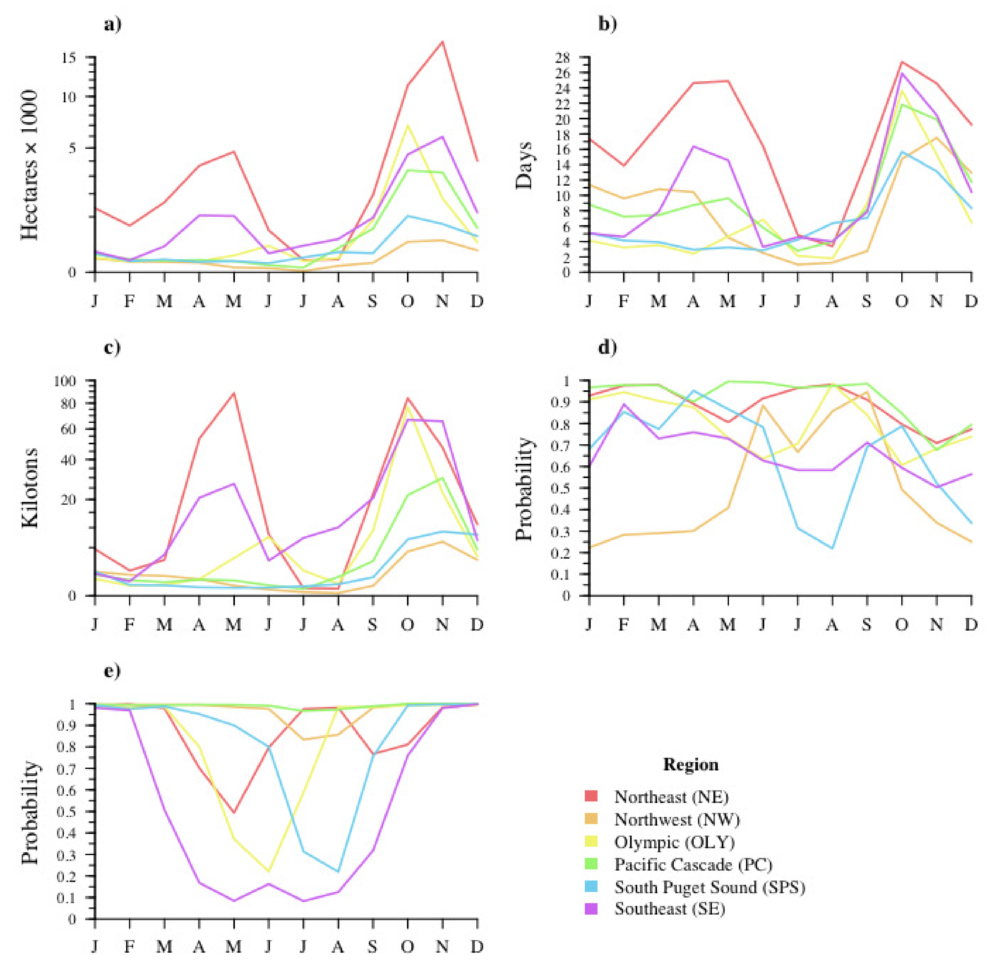
Figure 7.
The probability that each month will have the highest prescribed fire use for that year according to five prescribed fire parameters. Each panel corresponds to a DNR administrative region: Northeast (NE), Northwest (NW), Olympic (OLY), Pacific Coast (PC), South Puget Sound (SPS), and Southeast (SE).

Figure 8.
Differences in proposed burn characteristics by approval outcome for each DNR administrative region (Northeast (NE), Northwest (NW), Olympic (OLY), Pacific Coast (PC), South Puget Sound (SPS), and Southeast (SE)). Boxplots to illustrate the difference in area burned (a) and biomass burned (b) between approved and denied burns. The mosaic plots (c) illustrate the joint frequency of burns in approved-denied categories and pile-not pile categories. The significance of the differences and dependence levels, assessed with t-test and Chi-squared tests respectively, are denoted with asterisks. p-values greater than 0.03 are interpreted as not significant, p-values less than 0.03 are interpreted as significant, p-values less than 0.0075 are interpreted as strongly significant (**), and p-values less than 0.0005 are interpreted as very strongly significant (***). See Section 2.2.1 for details. For visualization purposes, area burned and biomass burned are square-root transformed, and outliers are removed from the boxplots.


Table 1.
Number of burn requests between 2004 and 2019, disaggregated by approval outcome and burn category for each DNR administrative region (Northeast (NE), Northwest (NW), Olympic (OLY), Pacific Coast (PC), South Puget Sound (SPS), and Southeast (SE)).
Table 1.
Number of burn requests between 2004 and 2019, disaggregated by approval outcome and burn category for each DNR administrative region (Northeast (NE), Northwest (NW), Olympic (OLY), Pacific Coast (PC), South Puget Sound (SPS), and Southeast (SE)).
| Region | Total | Approved | Category | |||
|---|---|---|---|---|---|---|
| Yes | No | Broadcast | Natural | Pile | ||
| NE | 23,181 | 19,100 | 4081 | 2578 | 1232 | 19,371 |
| NW | 2847 | 1020 | 1827 | 0 | 0 | 2847 |
| OLY | 6400 | 4310 | 2090 | 237 | 0 | 6163 |
| PC | 7730 | 6424 | 1306 | 9 | 0 | 7721 |
| SPS | 2951 | 1884 | 1067 | 9 | 160 | 2782 |
| SE | 7782 | 4642 | 3140 | 1061 | 1027 | 5694 |
Table 2.
Area and percent of DNR administrative regions (Northeast (NE), Northwest (NW), Olympic (OLY), Pacific Coast (PC), South Puget Sound (SPS), and Southeast (SE)). Total area and percent of Washington State that each DNR administrative region occupies are reported alongside the area and percent within the DNR administrative regions of each land ownership (public, private) and ecoregion category (Blue Mountains (BM), Cascades (C), Coast Range (CR), Columbia Plateau (CP), Eastern Cascades Slopes and Foothills (EC), North Cascades (NC), Northern Rockies (NR), Puget Lowland (PL), Willamette Valley (WV)). Areal measurements are in square kilometers.
| Region | Total | Ownership | Ecoregion | |||||||||
|---|---|---|---|---|---|---|---|---|---|---|---|---|
| Public | Private | BM | C | CR | CP | EC | NC | NR | PL | WV | ||
| NE | 35,892 (20%) | 15,406 (43%) | 20,485 (57%) | 0 (0%) | 0 (0%) | 0 (0%) | 7682 (21%) | 0 (0%) | 6789 (19%) | 21,420 (60%) | 0 (0%) | 0 (0%) |
| NW | 17,291 (10%) | 10,873 (63%) | 6418 (37%) | 0 (0%) | 0 (0%) | 0 (0%) | 0 (0%) | 0 (0%) | 12,091 (70%) | 0 (0%) | 5089 (30%) | 0 (0%) |
| OLY | 13,530 (8%) | 8132 (60%) | 5398 (40%) | 0 (0%) | 0 (0%) | 10,418 (77%) | 0 (0%) | 0 (0%) | 1544 (11%) | 0 (0%) | 1507 (11%) | 0 (0%) |
| PC | 18,571 (11%) | 7249 (39%) | 11,323 (61%) | 0 (0%) | 9579 (52%) | 5912 (32%) | 0 (0%) | 1 (<1%) | 0 (0%) | 0 (0%) | 1965 (11%) | 1068 (6%) |
| SPS | 15,200 (9%) | 5723 (38%) | 9477 (62%) | 0 (0%) | 4369 (29%) | 991 (7%) | 0 (0%) | 0 (0%) | 1214 (8%) | 0 (0%) | 8381 (56%) | 0 (0%) |
| SE | 74,942 (43%) | 25,269 (34%) | 49,674 (66%) | 2108 (3%) | 1959 (3%) | 0 (0%) | 53,936 (72%) | 8185 (11%) | 8753 (12%) | <1 (<1%) | 0 (0%) | 0 (0%) |
Table 3.
Annual trends in five prescribed fire parameters from 2004–2019 for each DNR administrative region (Northeast (NE), Northwest (NW), Olympic (OLY), Pacific Coast (PC), South Puget Sound (SPS), and Southeast (SE)). p-values greater than 0.03 are interpreted as not significant (ns), p-values less than 0.03 are interpreted as significant (*), p-values less than 0.0075 are interpreted as strongly significant (**), and p-values less than 0.0005 are interpreted as very strongly significant (***). See Section 2.2.1 for details.
| Region | Area | Burn Days | Biomass | Approvals | Pile |
|---|---|---|---|---|---|
| NE | −5.14 (***) | −7.80 (***) | −21.3 (*) | −0.0032 (ns) | −0.0047 (ns) |
| NW | 0.07 (ns) | 2.42 (ns) | 1.43 (**) | −0.0167 (ns) | 0.0003 (*) |
| OLY | −0.48 (ns) | −2.32 (*) | −5.68 (*) | 0.0132 (ns) | 0.0049 (**) |
| PC | −0.32 (ns) | −2.51 (*) | −2.91 (ns) | 0.008 (ns) | −0.0002 (ns) |
| SPS | −0.29 (ns) | −1.21 (ns) | −4.97 (**) | 0.0122 (ns) | −0.0051 (ns) |
| SE | −1.40 (**) | −2.11 (**) | −20.66 (***) | 0.0021 (ns) | 0.0037 (ns) |
Table 4.
The major and minor modes of the seasonal profile of prescribed fire parameters by DNR administrative region (Northeast (NE), Northwest (NW), Olympic (OLY), Pacific Coast (PC), South Puget Sound (SPS), and Southeast (SE)). The modal values are reported in the parenthesis. Area burned is reported in thousands of hectares and burned biomass is reported in kilotons.
| Region | Area | Burn Days | Biomass | Approvals | Pile | |||||
|---|---|---|---|---|---|---|---|---|---|---|
| Major | Minor | Major | Minor | Major | Minor | Major | Minor | Major | Minor | |
| NE | Nov (17.22) | May (4.71) | Oct (27.38) | May (24.88) | May (88.49) | Oct (84.17) | Aug (0.982) | Mar (0.979) | Feb (0.998) | Dec (0.996) |
| NW | Nov (0.33) | Nov (17.50) | Mar (10.81) | Nov (6.29) | Sep (0.946) | Jun (0.884) | Nov (0.999) | Mar (0.996) | ||
| OLY | Oct (6.99) | Jun (0.23) | Oct (23.62) | Jun (6.85) | Oct (77.10) | Jun (7.42) | Aug (0.985) | Feb (0.945) | Dec (0.995) | Mar (0.986) |
| PC | Oct (3.37) | Apr (0.05) | Oct (21.81) | May (9.62) | Nov (29.92) | Apr (0.56) | May (0.996) | Sep (0.985) | Nov (>0.999) | May (0.996) |
| SPS | Oct (1.03) | Aug (0.13) | Oct (15.69) | May (3.25) | Nov (8.9) | Apr (0.952) | Feb (0.854) | Dec (0.998) | Mar (0.988) | |
| SE | Nov (5.95) | Apr (1.05) | Oct (25.88) | Apr (16.38) | Oct (66.90) | May (26.99) | Feb (0.889) | Apr (0.760) | Dec (0.998) | Jun (0.163) |
Publisher’s Note: MDPI stays neutral with regard to jurisdictional claims in published maps and institutional affiliations. |
© 2021 by the authors. Licensee MDPI, Basel, Switzerland. This article is an open access article distributed under the terms and conditions of the Creative Commons Attribution (CC BY) license (https://creativecommons.org/licenses/by/4.0/).
Share and Cite
MDPI and ACS Style
Podschwit, H.; Miller, C.; Alvarado, E. Spatiotemporal Prescribed Fire Patterns in Washington State, USA. Fire 2021, 4, 19. https://0-doi-org.brum.beds.ac.uk/10.3390/fire4020019
AMA Style
Podschwit H, Miller C, Alvarado E. Spatiotemporal Prescribed Fire Patterns in Washington State, USA. Fire. 2021; 4(2):19. https://0-doi-org.brum.beds.ac.uk/10.3390/fire4020019
Chicago/Turabian StylePodschwit, Harry, Colton Miller, and Ernesto Alvarado. 2021. "Spatiotemporal Prescribed Fire Patterns in Washington State, USA" Fire 4, no. 2: 19. https://0-doi-org.brum.beds.ac.uk/10.3390/fire4020019