
Fine-Scale Fire Spread in Pine Straw


1
Department of Scientific Computing, Florida State University, Tallahasse, FL 32306, USA
2
Geophysical Fluid Dynamics Institute, Florida State University, Tallahassee, FL 32306, USA
3
Tall Timbers Research Station, 13093 Henry Beadel Road, Tallahassee, FL 32312, USA
*
Author to whom correspondence should be addressed.
†
Current address: 400 Dirac Science Library, Tallahassee, FL 32306, USA.
Fire 2021, 4(4), 69; https://0-doi-org.brum.beds.ac.uk/10.3390/fire4040069
Submission received: 20 August 2021
/
Revised: 28 September 2021
/
Accepted: 4 October 2021
/
Published: 10 October 2021
(This article belongs to the Special Issue Experimentation and Physics-Based Modeling to Support Prescribed Burning)
Abstract
:Most wildland and prescribed fire spread occurs through ground fuels, and the rate of spread (RoS) in such environments is often summarized with empirical models that assume uniform environmental conditions and produce a unique RoS. On the other hand, representing the effects of local, small-scale variations of fuel and wind experienced in the field is challenging and, for landscape-scale models, impractical. Moreover, the level of uncertainty associated with characterizing RoS and flame dynamics in the presence of turbulent flow demonstrates the need for further understanding of fire dynamics at small scales in realistic settings. This work describes adapted computer vision techniques used to form fine-scale measurements of the spatially and temporally varying RoS in a natural setting. These algorithms are applied to infrared and visible images of a small-scale prescribed burn of a quasi-homogeneous pine needle bed under stationary wind conditions. A large number of distinct fire front displacements are then used statistically to analyze the fire spread. We find that the fine-scale forward RoS is characterized by an exponential distribution, suggesting a model for fire spread as a random process at this scale.
1. Introduction
In many wildland and prescribed fires, the fire is spread through ground fuels. A typical ground fuel in these fires is dispersed pine straw beds, as pine forests are common native habitats across large areas of continental landscapes. Various factors determining the rate of spread (RoS) in pine straw, as well as many other fuels, have been condensed into fuel models that produce a single RoS value under given conditions (e.g., fuel model TL8 in Scott and Burgan [1]) via a fire spread model (e.g., Rothermel [2]). As is well known, these spread rates are typically based on uniform conditions and are not meant to represent local variations of spread in the full range of fuels and wind variability experienced in the field. Because of the turbulence and complexities of surrounding fire dynamics, characterizing fire spread under realistic conditions is challenging. Cruz and Alexander [3] analyzed a large number of fire spread models and observations, and the level of uncertainty that they reveal demonstrates the need for further understanding of fire RoS in realistic settings. Alexander and Cruz [4] also discuss the most important factors in fire behavior, such as fuel conditions, topography, and weather. While a laboratory setting allows for detailed small-scale measurements to be made, key environmental factors, such as fuel density variations, wind turbulence, and solar radiation are often absent. At the same time, field measurements of prescribed fires emphasizing the larger scale aspects of spread may not resolve important small-scale features [5].
This work investigates low intensity fire spread in a 2 m × 2 m pine straw fuel bed. Fire spread, even in the low intensity limit, is continuously changing in space and time. Therefore, rather than characterizing fire spread in terms of a single number, there is a need for statistical descriptions of the RoS in a natural, open environment. To form meaningful statistical properties of the RoS, it is necessary to measure velocity at a high resolution in both space and time across the flaming region. Very high-resolution fixed-point observations have been acquired in numerous experiments and demonstrate the rapid evolution of heat fluxes [6]. The movement of the combustion zone or burning front within the fuel, as opposed to the flaming gases, generally occurs at lower speeds, yet rapid jumps and bursts nevertheless occur.
Laboratory studies of spread and heat release rate have also been conducted using infrared and visible images. Using visible imaging and heat flux sensors, Tihay et al. [7] produced estimates of spread and heat release rate (HRR) in maritime pine (Pinus pinaster (Ait.)) straw. For no slope and no wind, an RoS of m/s was found with a bed loading of . The corresponding HRR was roughly 100 kW per meter of fire front. A similar setup was used by Schemel et al. [8], who related the time of ignition, duration of combustion, and peak HRR with analysis of variance techniques. Similar to this work, Martínez-de Dios et al. [9] made infrared and visual recordings of a pine straw fuel bed with experiments performed indoors and with slope. After applying computer vision techniques, they report flame height and basic statistics (mean and variance) of the position and shape of the fire front. As a post-processing step, they computed the RoS, but only of the leading and rear edge of the fire front. Zhou et al. [10] applied a thermal particle image velocity algorithm to infrared video to estimate velocities of the gases near a combusting region in an indoor laboratory.
Infrared and visual video have been widely employed to characterize fire spread in natural settings. Linn et al. [11] investigated downwind RoS in the 2012 RxCADRE prescribed burns from observations and with numerical simulations. The RoS results were compared to wind data collected from a comprehensive suite of sonic anemometers. Large variations in the RoS were found with no correlation to measured wind. These results were attributed to the dependence of the RoS on fire ignition patterns. Stow et al. [12] used infrared images captured of wildfires to compute fire spread rates. Since they investigated large wildfires, their approach operates at a much coarser resolution than laboratory or typical prescribed fire experiments. They manually determined the flaming front locations of each image and the displacement vectors between consecutive images. Prohanov et al. [13] developed algorithms to detect and track firebrands. They also provide errors, but they do not provide statistical distributions of their data. Morandini et al. [14] implemented particle image velocimetry (PIV) to develop techniques to measure the turbulent wind velocities in and around a fire with video camera mounted on the ground. Their initial results show the dependence of flow within the fire on the buoyancy regime, with transitions from strong vertical to horizontal flow.
In one of the most detailed prescribed fire RoS studies, Paugam et al. [15] used infrared cameras, in one case mounted 10 m above a 1 m × 1 m plot, and in another on an helicopter pointed at a 45 m × 21 m natural fuel bed. For the larger burn, they estimated the RoS by assuming that the fire spreads in the normal direction. A later paper [16] showed that this method agrees well with an accepted standard for RoS that is computed with a thermocouple grid array. Clements et al. [17] made several measurements of a prescribed fire of 155 acres of grassland. Measurements were made using IR video, sonic anemometers, thermocouples, and sodars, and the data were used to calculate in situ turbulence and moisture enhancement within a grass fire. Very intense wildland fires have been studied by Coen et al. [18] and Clark et al. [19] using infrared imagery to explore crown-fire dynamics of the FROSTFIRE experiment carried out in Alaska. They apply image flow analysis to infrared images of the fire, but at a distance of more than 2.5 km from the combustion zone. By assuming that the temperature field is transported solely by the wind they calculate the wind velocity along with fire front characteristics.
An interesting application of stochastic methods to fire spread was performed by Zhang et al. [20] who developed a stochastic model for a very small-scale paper burning experiment. Their results lend support to the idea that the small-scale frontal motion is a chaotic process. The approach outlined below leads to a statistical description of the small-scale chaotic spread in a simplified but realistic setting. This approach provides a similar, but alternative view of fire spread as a random process, as a step toward a more complete physical and statistical framework for fire spread in the complex natural environment.
Section 2 explains the experimental setup and the data that are collected. The videos are captured by a visual camera and an infrared camera mounted above the fuel bed to compute velocities. To convert the infrared images to velocities, computer vision techniques are applied to individual frames. Because of the chaotic nature of the frontal motion, standard computer vision techniques require modification. Our algorithm first defines a single-pixel-wide approximation of the combusting region of each frame. This is performed by segmenting and cleaning each frame, and then finding the shortest path passing through the combusting region. Then, the assignment problem between consecutive frames is solved, and this defines the displacement vectors of the fireline that are then converted to velocities. The computer vision techniques that are applied are described in Section 3. Using this methodology, velocity and burn time distributions are generated and discussed in Section 4. A discussion of the results is presented in Section 5.
2. Data
The data used in this paper were recorded in the early afternoon of 22 November 2019 at the Tall Timbers Research Station in northern Florida (see Figure 1). The reported ambient temperature was C with a relative humidity of and a mean wind speed of 1.3 m/s with gusts up to 3 m/s. Meteorological data were collected using a Campbell Scientific automatic weather station (Campbell Scientific, Inc. Logan, UT) located at Tall Timbers Research Station. A 2 m × 2 m bed of dry long-leaf pine straw with a moisture content of about 15% was constructed by hand. The density distribution of needles was made roughly uniform by re-arranging needles for a visibly constant depth of 10 cm and apparent average needle separation. No obvious gaps or hollows were apparent. We refer to this as quasi-homogeneous to distinguish it from a perfectly uniform fuel bed (e.g., Bebieva et al. [21]). The fuel bed was marked with metal pieces at each corner of the plot. The corners are marked so that they can be used in conjunction with the camera resolution to determine the physical dimensions of a pixel. A low-temperature infrared image of the setup was taken before the prescribed burn to capture the location of the metal corners in the infrared camera’s frame; the cool metal corners are difficult to discern once burning takes place. After capturing this reference image, the infrared camera’s lower limit was set to record temperatures at or above C. Large metal sheets were placed to block crosswinds and minimize their effect on the direction and RoS. A fan was placed approximately 7 m behind the setup and blew in the direction of the ambient wind. The fan was used to maintain a stationary and roughly uniform wind field and made strong enough to guarantee that a head fire was present at all times. The resulting experimental wind direction is shown in Figure 1.
The ambient wind speed and fan speed combined to produce an overall mean wind speed estimated to be m/s, causing the flame to stretch and tilt as described in Section 4. Some variations occurred as small gusts in the ambient wind. The wind speed estimation calculations are described below. The experiment took place on flat ground, with negligible slope effects. A drip torch was used to ignite a line along the lower portion of the plot. The fire does not reach the end of the fuel bed at a fixed time, but rather over an interval from about 50 s to 80 s. This implies rates of spread ranging from 2–4 cm/s.
A visual camera and an infrared camera were situated on a tripod 6 m above the plot, looking straight down. This is a similar setup as others (O’Brien et al. [22]; Loudermilk et al. [23]). The time variable is calibrated using the frame rate of the cameras. The visual video was captured using a Hero 7 Silver (GoPro, Inc., San Mateo, CA, USA) recording at 30 Hz, and the infrared video was captured with a FLIR A655sc camera (Teledyne FLIR, LLC., Wilsonville, OR, USA) recording at 1 Hz, an emissivity of 0.95, and a spectral range of 7.5–14.0 m. The temperature range of the infrared camera was 100–900 C. Since the visual camera has a higher frame rate than the infrared camera, it resolves shorter time scales and higher frequencies. The temperature calculation from emitted radiation assumes a constant emissivity, while the emissivity of the various components of the fire environment, unburnt fuel, burning fuel, flames, and gases, varies (e.g., Agueda et al. [24]). As our methodology tracks the neighborhood of an individual isotherm of a single component it minimizes the effect of variations in emissivity.
Frames sampled at approximately 10 s intervals from the visual and infrared videos are shown in Figure 2. In the visual images, the black, apparently burnt areas are still undergoing combustion underneath a superficial char layer. This confined layer of burning fuel is fanned by the movement of the ambient wind through the fuel and produces intense heat and high temperatures. The IR camera reveals these high temperatures of the fuel surface and hot gases emanating from the combustion layer. Note that the remnant charred fuels in Figure 2 have attained their maximum surficial temperature and have only just begun cooling according to their temperature time series.
Wind speed at flame height is roughly estimated using the movement of the smoke plume between frames. Three example points identified in successive frames are sampled from portions of the plume away from the combusting region (Figure 3); this is carried out to minimize motions away from the surface caused by thermal radiation and turbulent flame motion. The change in longitudinal position is calculated for each set of points, and then converted to a velocity using the time between visual frames. The three velocities calculated were m/s, m/s, and m/s for the cyan, green, and yellow points, respectively. The average of these three samples gives a wind speed of m/s along the positive longitudinal axis. Since the smoke is still buoyant and rises between frames, an error of m/s was calculated using other possible positions for the second set of points in Figure 3. The smoke parcels chosen were near flame height, so the estimated wind speed is appropriate for the flame height region. At this height, the wind speed values m/s are generated by both the ambient wind and fire-induced winds. While this estimate for the wind speed is rough, its purpose is not to calculate the spread, but rather to validate estimates of the flame tilt angle.
3. Methodology
To investigate fire propagation at high spatial resolutions, computer vision and graph theory algorithms are used to calculate velocities of the fireline. Computer vision applied to motion analysis is a mature subject, but it assumes that the frame rate is sufficiently high to capture the environment’s dynamics. Prescribed fire environments are turbulent and the frame rates of cameras deployed in these environments are typically too low to capture all the dynamics. Therefore, classic computer vision algorithms are modified so that velocities in the environment can be reliably estimated. This includes modifying methods to segment and clean the frames via thresholding [25], find isotherms, and track the isotherms’ motion. In the coming sections, these modified algorithms are described for videos captured with either a visual camera or an infrared camera. The head fireline has an upwind and downwind side, and we characterize the spread of the upwind side (see Figure 4). The upwind side has, as described below, less variability and a more stable representation of the fire front. In contrast Paugam et al. [15] calculated the spread of the downwind side of the flaming region (see also Johnston et al. [16]).
3.1. Segmenting Fuels, Active Combustion, and Gases
Individual frames captured with a visual or an infrared camera must first be segmented into meaningful regions. The natural regions are burning fuels, the active flaming region, hot gasses being transported through the atmosphere, and fuels that are not yet burning. Visual images capture surface areas of burning fuel, the flaming region, unburnt regions and smoke, whereas infrared images capture radiation from burning fuel that may be heating up (growth stage) or cooling (decaying stage), preheated (unburnt) fuels, and heated gas and particles. Separating frames into these regions allows the dynamics of the fireline and the growth of the fire scar to be tracked.
Due to stark differences in color between elements in fire videos, standard color segmentation is sufficient to segment visual images. The segmentation algorithm starts by choosing characteristic pixels in a single frame that represent each of the three regions. A pixel is then defined to be charred burning fuel, actively combusting, or a hot gas if each of its RGB channels are within a specified tolerance of the corresponding characteristic pixel. Portions of an image that are not categorized into one of these regions are considered unburnt fuel, and these points are not of interest. These points include vegetation that is sufficiently downwind from the combustion region. A visualization of the points that are classified as combusting is shown in Figure 5.
Infrared images are segmented using temperature values. To determine appropriate threshold values, knowledge of the fuels’ combustion properties is required. For example, in the controlled burn in Figure 1, the fuel ignites at approximately C and reaches temperatures greater than C when burning [26]. Simeoni et al. [27] used a slightly higher threshold temperature for the burning zone of C. Because of the large gradients in the temperature, other reasonable choices for the ignition temperature do not have a significant effect on the results.
Appropriate temperature thresholds can be found by analyzing temperature data at fixed points or by observing the segmented frames resulting from different thresholds. In a given frame, each pixel above the ignition temperature is classified as a burning pixel. Pixels that are heated but have yet to reach the ignition temperature are classified as hot gases and pre-heated fuels. Pixels exceeding the ignition temperature and below the maximum temperature are classified as fully combusting. Finally, pixels that have exceeded the ignition temperature and have begun to cool from their maximum temperature are classified as charred. These categories are illustrated in Figure 6. Infrared images allow the introduction of cooled fuels as a subcategory of charred fuel, as they are able to detect and track the cooling rate of charred fuel. Pixels that have reached their maximum recorded temperature, which ranges between C and C, are first colored in red. They are colored in dark brown after they have cooled below C. The typical time series of a pixel’s temperature is in the right plot of Figure 4. We focus on the region between charred and combusting fuels in order to better represent the fire front.
3.2. Cleaning the Segmented Images
To help identify a single fire front within each frame, the segmented image must be cleaned. The goal is to isolate the main body of fire from the numerous small regions of hot gases and embers that are continuously emitted. The cleaning process requires the segmented image matrix, a search radius, and a threshold. The cleaning algorithm loops through each pixel with a nonzero intensity in the segmented image and determines the number of nonzero pixels within the user-defined radius. If the number of nonzero pixels exceeds the user-defined threshold, the pixel is deemed to be part of the main body of the fire, and therefore a relevant pixel for fire spread calculations. If the total count falls below the threshold, that pixel is deemed outside the main body of the fire. The thresholds are determined by testing the algorithm on a single frame’s segmented fire image matrix before applying it to the entire video. This cleaning process returns a logical mask consisting of 0 s and 1 s that correspond to isolated pixels and the main body of the fire, respectively. Figure 7 shows cleaned versions of sample segmented frames from Figure 5 and Figure 6. In these frames, the cleaner has removed small patches of heated fuel (gray) on the top left corner of the infrared image, and small patches of combusting cells on the bottom of the visual image.
3.3. Isolating the Fire Front
After the cleaner removes small regions that are disjointed from the main body of fire, the edges of the cleaned image need to be formed. Edges are pixels with large gradients in image intensity, and these are typically found with convolutions and thresholding applied to the pixel intensity [28]. Before calculating gradients of the image, the logical mask is combined with the original image; the original image matrix’s pixel intensity values are changed to zero in every index where the logical mask is 0. By applying this pre-processing step, only edges of the combusting region will be sought.
After experimenting with different edge detection operators including Prewitt [29], Sobel [30], and Roberts Cross [31,32] in combination with Gaussian filtering, we determined that the Sobel edge detection operator achieves the best balance between fine detail detection and computational expense on sample fire environment images. The Sobel operator applies a two-dimensional central difference and intensity threshold to estimate the image gradient. After the convolution process, we reassign a value of zero to all pixels that originally had zero intensity. Figure 8 shows a segmented and cleaned image (left), and the result of edge detection (right). In the left plot, points that have been pre-heated, ignited, or burnt are in white. The dark brown region is the burning region that has begun to cool, while the orange region is the actively flaming region. The right plot shows the edges between the heated gases, combusting region, and burnt area.
Figure 9 is a zoom of the middle third of the right plot of Figure 8. Note that the edges are often several pixels wide. However, to track the motion of the edges, a clean one-pixel-thick isotherm that represents the fireline is preferred. Using ideas from graph theory, an algorithm called Crawler defines this one-pixel wide edge. Crawler uses an adaptation of Dijkstra’s algorithm [33] to form the shortest path between two endpoints of the isotherm. Sets of points in each frame are labeled according to temperature region; for infrared images, this is completed using temperature data and for visual images, this is completed using burning state (see Section 3.1). If all points in a region are connected, the start and end points for Dijkstra’s algorithm are detected automatically by finding the uppermost point at each end of the region. However, because of the ignition pattern, early frames consist of several disjoint sections of burning fuel. Therefore, as a pre-processing step, these regions are connected before Crawler is used to define a fireline. Crawler also crops the image according to the location of nonzero pixels connected to the endpoints. Though this requires another loop through each video frame, the number of points accessed in later steps (Section 3.4) is reduced and the code runs significantly faster. Crawler also assigns each pixel a physical coordinate so that future calculations are physical rather than image-based. Successive firelines found with Dijkstra are superimposed in the left plot of Figure 9, and their conversion to physical coordinates are in the right plot of Figure 9.
3.4. Displacement through Assignment
Once Crawler has identified firelines of every frame, a correspondence between points on the firelines from consecutive frames is defined. Since ignition by embers is not observed, points on a fireline are ignited by a nearby point from the previous frame. This correspondence results in displacement vectors which are converted to velocity vectors by multiplying by the camera’s frame rate. Letting A and B be the set of fireline points in consecutive frames, the displacement vector originating at could be defined as , where minimizes the energy
This is the classic assignment problem, but two modifications for the problem at hand are made.
Given the spatial and temporal resolutions, large displacements are not expected, implying small motions between successive frames. Making use of this assumption, we define the subsets of A
where , is an interval subset of the camera’s x field of view, and is defined analogously. We seek a collection of mappings that minimize
where
By requiring and , the displacement vectors are not unphysically large. The intervals are chosen to all have the same size, and to avoid edge effects, they are arranged so that the left and right thirds overlap with neighboring intervals so that there is a buffer zone (see Figure 10). Because of the overlap, can be contained in two neighboring sets, and . When this happens, Equation (4) considers both and , and the smaller of the two defines in Equation (3). To determine an appropriate size for the intervals , the data are used to determine an appropriate length scale. After subtracting the mean value, the first zero crossing of the autocorrelation of the y coordinate of a sample isotherm defines the interval size. The large negative lobes in both regions are suggestive of larger scale coherent meandering of the fire front, associated with eddies and whirls. These effects are beyond the scope of the present analysis and will be reported later. The autocorrelation of sample isotherms is shown in Figure 11 and the first root is denoted by the blue circle. Using this interval size results in the intervals illustrated in Figure 10.
The second modification is required since the number of points in and are likely different, and this results in an unbalanced assignment problem. To balance the problem, nodes with weight 0 are added to the set containing fewer points. These nodes participate in the assignment problem, but a 0 weight means they do not influence the energy Function (1).
To solve the modified assignment problem, the classic assignment problem is solved in each subdomain. These local problems are solved by converting the assignment problem to a linear program that is solved with the Simplex method. Sample displacement vectors between consecutive isotherms are in Figure 12. To demonstrate the importance of choosing appropriate interval sizes, the modified assignment problem with much smaller and larger interval sizes are considered. Interval sizes that are too small result in large gaps with no displacement vectors, while interval sizes that are too large result in unphysical displacement vectors.
3.5. Algorithmic Complexity
Here, the computational cost of the algorithms described above are discussed. All calculations are performed on a standard laptop computer. Each frame consists of N pixels, and a typical fireline contains pixels. The standard computer vision tasks of segmentation, cleaning, and edge detection each require operations. The Crawler, which is applied using Dijkstra’s algorithm, requires operations. Finally, the assignment problem is solved using the Simplex method, and the implementation requires operations.
4. Results
We form and analyze velocity distributions from the experiment and methods described in Section 2 and Section 3. These velocities are decomposed into the longitudinal direction (in the direction of the wind) and the transverse direction (perpendicular to the wind). Velocities are taken over 67 frames, and this results in 10,858 velocity samples. The first 15 s after the ignition pattern is laid down is ignored to allow the fire to form into a single head fire. A large number of velocities are recorded as 0 cm/s, and this is an artifact of the spatial and temporal resolutions of the experiment. In particular, the camera can view pixels per centimeter, meaning the spatial resolution is cm. Since the infrared camera has a sampling rate of 1 Hz, any velocity below cm/s will be recorded as 0 cm/s. Investigating smaller velocities requires a camera with a higher spatial resolution and sampling rate.
Figure 13 shows the probability distribution of the non-zero longitudinal (left) and transverse (right) velocities on a logarithmic scale (top) and linear scale (bottom). The mean longitudinal velocity is cm/s which can be interpreted as an average RoS, and its distribution is dominated by positive values since the positive direction corresponds to the downwind propagation of the head fire. Negative longitudinal velocities make up of the total distribution, and these negative velocities are caused by small scale turbulent behavior that is discussed in detail in Section 4.2. The distribution of transverse velocities is symmetric, and its mean velocity is cm/s, which is below the sampling threshold of the experimental setup. Therefore, the transverse velocity mean is effectively 0 cm/s, indicating that there is no clear preference in the transverse spread direction. This is consistent with a quasi-homogeneous fuel bed, and negligible mean cross-wind flow. Note that both the longitudinal and transverse velocity distribution deviate from Gaussian.
The standard deviation and kurtosis of the velocity field in both directions are also reported in Figure 13. The ratio of the standard deviation to the mean, 1.4, is a rough measure of frontal bursts, suggesting that the RoS fluctuates strongly around the mean. The physical reasons for this fluctuation are discussed in Section 4.3. We focus on spread in the direction of the mean wind by only considering the longitudinal velocity. Note that the transverse velocities are important if considering, for example, the speed in the direction of frontal movement.
The maximum measured velocity can be bounded by considering the maximum flame length. In the experiment, the maximum observed apparent flame length in any one frame is less than approximately 40 cm. Given the frame rate of 1 Hz, velocities larger than cm/s are not observed in Figure 13. Such large velocities are extremely rare, yet appear on the logarithmic scale as a rough cut-off in longitudinal velocity. Physically, this is related to the time-scales of pyrolysis and advection of burning gases by the wind.
4.1. Positive Longitudinal Velocities
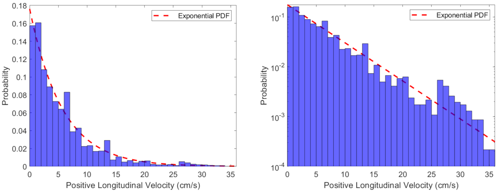
Positive longitudinal velocities are used to describe the overall RoS of the primary frontal zone. Ignoring the negative values, mainly due to fluctuating hot gases and temporary isolated backing fires (Section 4.2), the distribution of the positive longitudinal velocities are plotted in Figure 14. The resulting values have a mean and standard deviation of cm/s and cm/s, respectively, and these depend on several factors, including the homogeneity of the fuel and the background wind. For comparison, Morandini et al. [14] described fire front position in a similar fuel bed and showed a nearly uniform RoS of approximately 6 cm/s for 60 s. Using the measured mean velocity, an approximate exponential distribution is observed (Figure 14). The normalized root mean square error is cm/s. Both linear and log scales are used to display the behavior; higher values at the tail are apparent, possibly due to the sampling limitations at a high velocity.
Relatively high resolution RoS observations were obtained by Paugam et al. [15] using IR cameral images of an experimental small-scale fire and a larger scale prescribed fire. Their method determined a first arrival time based on a pixel temperature threshold. For the larger fire, the spatial resolution was 18 cm × 18 cm, but this was further averaged to 1.44 m × 1.44 m to reduce noise in the calculation and to produce maps. Statistical distributions of these data were presented by Johnston et al. [16] and appear to support an exponential form. Initial calculations (not shown) using data derived from the RxCadre experiment (Hudak et al. [34]; Butler et al. [35]) also support exponential behavior at low to moderate RoS.
4.2. Effects of the Flame Dynamics
Most of the longitudinal velocities in Figure 13 are positive and no larger than 15 cm/s, which is a little less than two standard deviations from the mean value. However, large and negative velocities were observed that are significant. The majority of these large and negative velocities can be explained by considering how the flame dynamics affect fire spread velocities. In particular, as the flame oscillates back and forth in the turbulent atmospheric environment, both direct flame contact and flame radiation create large and negative velocities [36,37]. Maynard et al. [38] also showed that large velocities are created when two firelines merge, which may happen in either sense (positive or negative).
Large velocities are also created whenever a new disconnected combusting region forms away from the main fireline. Some of these new regions can be up to 40 cm from the main fireline and are created by flame contact. Another process that creates disconnected combusting regions occurs when hot gases or flames propagate underneath the top layer of the porous fuel bed structure, and then reappear away from the main fireline. Initially these disconnected regions are not considered since the algorithm defines a single, continuous fireline. However, once these regions reconnect to the main fireline, the result is an isotherm that has undergone a large hop, and this is recorded as artificially large velocities. This effect is quantified by considering flame lengths between 15 cm and 40 cm igniting patches of fuel by either direct flame contact or flame radiation. These methods of propagation are responsible for velocities whose magnitude are greater than 15 cm/s, and this value depends on wind speed, inclination, and fuel properties such as the fuel thickness [27,37] and porosity [21]. Note that our methods interpret this hopping phenomenon and spotting similarly, but spotting was not observed in the experiment. A different experimental setup, including the fuels, fire intensity, and plot size, would be required to investigate spotting.
The presence of negative longitudinal velocities are also explained by considering what the isotherm represents—part of a frontal zone comprised of burning material with fluctuating temperatures. That is, the isotherms are representative of the frontal zone, but the zone itself does not contain an exact, uniquely defined fire front line. Consequently, another source of negative velocity values is the existence of occasional small backing fires throughout the burning region. Despite having a roughly homogeneous fuel bed, neighboring pieces of fuel will not always ignite in immediate succession. This can be caused by factors such as fuel moisture [39] and local wind velocity [40]. In the experiment, negative values occur when material in the lower region of the frontal zone becomes heated and ignites after the material toward the top of the frontal zone has begun to cool. This is expected for fire fronts with fuels that are subject to turbulence in the surrounding air, such as pine straw beds [41]. A detailed examination of the frames indicates that the turbulent flame oscillations make up the majority of the negative longitudinal velocities.
Ignition by both flame radiation and direct contact depend not only on the flame length, but also the flame tilt angle. The flame tilt angle is estimated by considering the apparent maximum flame length and ambient wind speed. Using a wind velocity estimate of m/s in conjunction with the results of Morandini et al. [37], an estimate of the total flame length is between 59 cm and 74 cm. With these lengths, the tilt angle is calculated to be between and . This is consistent with the conclusion of Albini [42], who argued that flame tilt angles in pine straw do not normally exceed about .
4.3. Burn Time and Arrival Time
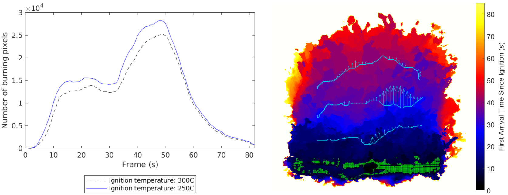
Once a pixel ignites, another important variable is the burn time, which is related to the rate of fuel consumption. The burn time is defined to be the time from a pixel’s ignition until it reaches its maximum temperature. Using two different choices of ignition temperature, we plot the number of burning pixels of each frame in the left plot of Figure 15. Both ignition temperatures are plausible for pine straw, and the choice of one over the other produces little variability in the overall shape.
From the start of ignition until approximately 10 s, a rapid increase in the number of burning pixels to about is observed. This increase is completely attributed to the ignition pattern that resembles a small open loop (see green points in the right plot of Figure 15). Since this region resembles a small ring fire, the unburnt fuel surrounded by the ignition pattern is quickly ignited. After 10 s, pixels begin to burn out, while new pixels, mostly located at the head, are ignited. For about 20 s, pixels are extinguished and ignited at a nearly constant rate, resulting in a nearly constant number of burning pixels. Then, at around 35 s, there is another increase in the number of burning pixels, associated with a sudden increase in the flame length, which we expect is caused by an ambient wind increase. Further evidence of this wind increase is shown in the right plot of Figure 15 where large velocities of the isotherm at s are observed. Finally, after about 50 s, flames begin to reach the boundary of the fuel bed, and the number of burning pixels begins to decrease. However, combustion continues until about 80 s.
The temperature history of each pixel suggests another way to understand fire spread, by determining the first instance each fuel parcel ignites—this is commonly called the first arrival time [43]. The first arrival time is computed by determining the first time each pixel exceeds the ignition temperature of C. The first arrival time of the experimental burn is illustrated in the right plot of Figure 15, also showing firelines and the spread velocity at three instances. Both an overall linear fire spread pattern in the direction of the wind (bottom to top) and also the slow moving backing fires discussed in Section 4.1 are observed. As the ignition line is not exactly on the upwind edge of the fuel bed, the fireline travels approximately 170 cm in the longitudinal direction to reach the end of the bed. From the range in final arrival times, one obtains a range in RoS roughly between 2–4 cm/s. These net RoS values do not reflect the bursts of higher velocity that arise during the complex movement of the front, raising the mean in the distribution (Figure 13) of instantaneous values.
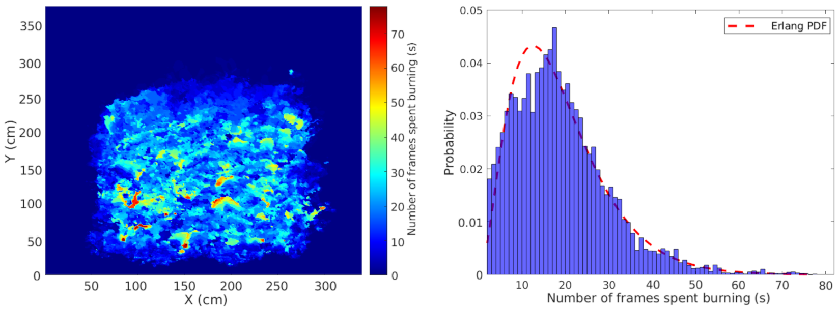
The fuel and atmospheric conditions not only affect the size of the combustion region and the RoS, but also condition the burn time. A heat map of the burn time and its corresponding probability distribution shows that the burn time is far from uniform, with clusters of longer times distributed apparently randomly over the fuel bed (Figure 16). These clusters presumably firstly represent variations in fuel density, with slightly higher packing, slight composition differences (no pine cones were present), or thickness, and secondly periods of lower wind or higher moisture with correspondingly reduced rates of combustion. We suggest that small-scale turbulent wind effects exert the largest control on burn time in this quasi-homogeneous fuel bed.
The histogram resembles distributions observed in the 2012 RxCADRE burns [44] (for more details on the RxCADRE burns see [22,45]). The data are fit to an Erlang distribution with shape parameter k and rate parameter . To determine the best fit, the value of that minimizes the normalized root mean square error for is found. Values larger than did not result in a good fit. The smallest normalized root mean square error is s with shape and rate parameters and , respectively. The relevance of this distribution can be understood as a model fundamentally derived from the exponential spread rate, itself a result of the interaction of turbulence and thermodynamic combustion processes. Hence, once ignited, the time of arrival of an extinction front or event follows from the sum of the displacements of intermediate isotherms, which produces an Erlang distribution. Of course, the parameters of the model depend on the fuel, atmospheric, and other environmental conditions.
5. Discussion
Temperature data collected from a small 2 m × 2 m plot of pine straw were used to derive statistical distributions of dynamical and thermodynamical quantities, including the RoS and fuel burn time. This approach leads to a statistical description of small-scale fire spread as a random process. Clearly, additional high-resolution observations with different fuels and fuel loading and structure, other turbulent wind characteristics, and a broader range of environmental conditions are needed, but the methodology and statistical description presented here are expected to provide new insight into the fire spread process.
The distribution for the forward RoS is exponential, consistent with an independent frontal inter-arrival time random process. The observations of fine-scale RoS differ dramatically from a spatially and temporally averaged RoS. The recognition that fire spread is subject to driving by wind turbulence at small scales as well as at larger scales, and the impact of random fluctuations in fuel bed characteristics, helps to explain the fine-scale variations in space and time. Initial comparisons to larger scale prescribed fire statistics suggests that the results scale up and that IR observational techniques are a promising route to improve models of fire spread.
The observation of the Erlang burn time distribution can be interpreted as an underlying random process for extinguishing events. However, it can also be interpreted as the convolution between multiple exponential distributions for the combustion time of a given fuel element. More general conditions may be represented by a non-homogeneous Poisson process, for which the rate parameter varies in time. This speaks to the complex processes that play into fire spread, but also the useful synthesis that a statistical description provides.
Datasets such as the one we collected can be combined with machine learning techniques to develop data-driven models for prescribed fire dynamics. For example, Hodges et al. [46] used convolutional neural networks to estimate the time-resolved spatial evolution of wildland fire. The deep convolutional network was trained on burn maps from data simulated from Rothermel RoS and FARSITE. However, the model is trained on semi-empirical models rather than experimental data. Chetehouna et al. [47] used an artificial neural network to estimate the RoS, flame height, and flame tilt angle in pine needle beds. In future works, we plan to use high-resolution datasets such as the one we have collected to train machine learning models that can be used to parameterize small-scale dynamics.
It is important to recognize that a statistical description does not preclude the use of underlying physical balances, or physical models, for deterministic constraints on the spread. In fact, such models are a necessary part of a more complete representation of fire spread in the complex surface fuel and atmospheric boundary layer. Hence, an alternative use of datasets such as the one we collected is to couple it with a physics-based model through data assimilation. This approach is taken by Zhang et al. [48], where they use a data-driven wildland fire spread model (FIREFLY) introduced by da Silva et al. [49]. Zhang et al. [50,51] used data assimilation to estimate state parameters and spread from the 2012 RxCADRE controlled burn experiment. Progress on data assimilation and machine learning techniques requires building relevant physical and statistical fundamentals into the methodology. Otherwise, it is unlikely that any amount of data can adequately train the system and produce a model capable of responding to the highly variable and complex natural environment.
Author Contributions
Conceptualization, D.S., K.S. and B.Q.; methodology, D.S., K.S., S.P. and B.Q.; software, D.S. and B.Q.; validation, D.S., K.S. and B.Q.; formal analysis, D.S., K.S. and B.Q.; investigation, D.S. and S.P.; resources, S.P.; data curation, D.S.; writing—original draft preparation, D.S., K.S. and B.Q.; writing—review and editing, D.S., K.S. and B.Q.; visualization, D.S.; supervision, K.S. and B.Q.; project administration, S.P. and B.Q.; funding acquisition, K.S. and B.Q. All authors have read and agreed to the published version of the manuscript.
Funding
This research was supported by the U.S. Department of Defense, Strategic Environmental Research and Development Program under Award Number RC20-1298; by the Geophysical Fluid Dynamics Institute, Florida State University; and by Tall Timbers Research Station.
Data Availability Statement
The data presented in this study are available on request from the corresponding author.
Acknowledgments
We would like to thank Tall Timbers Research Station who assisted with the experimental setup and performed the control burn. We also thank Peter Beerli for suggesting an Erlang fit to burn times.
Conflicts of Interest
The authors declare no conflict of interest.
References
- Scott, J.H.; Burgan, R.E.; Scott, J.H.; Burgan, R.E. Standard fire behavior fuel models: A comprehensive set for use with Rothermel’s surface fire spread model. In Technical Report General Technical Report RMRS-GTR-153; USDA Forest Service: Fort Collins, CO, USA, 2005. [Google Scholar]
- Rothermel, R.C. A Mathematical Model for Predicting Fire Spread in Wildland Fuels; USDA Forest Service Research Paper INT; Intermountain Forest & Range Experiment Station, Forest Service, US Department of Agriculture: Fort Collins, CO, USA, 1972; Volume 115. [Google Scholar]
- Cruz, M.G.; Alexander, M.E. Uncertainty associated with model predictions of surface and crown fire rates of spread. Environ. Model. Softw. 2013, 47, 16–28. [Google Scholar] [CrossRef]
- Alexander, M.E.; Cruz, M.G. Limitations on the accuracy of model predictions of wildland fire behaviour: A state-of-the-knowledge overview. For. Chron. 2013, 89, 370–381. [Google Scholar] [CrossRef]
- Clements, C.B.; Kochanski, A.K.; Seto, D.; Davis, B.; Camacho, C.; Lareau, N.P.; Contezac, J.; Restaino, J.; Heilman, W.E.; Krueger, S.K.; et al. The FireFlux II experiment: A model-guided field experiment to improve understanding of fire-atmosphere interactions and fire spread. Int. J. Wildland Fire 2019, 28, 308–326. [Google Scholar] [CrossRef] [Green Version]
- Frankman, D.; Webb, B.W.; Butler, B.W.; Jimenez, D.; Forthofer, J.M.; Sopko, P.; Shannon, K.S.; Hiers, J.K.; Ottmar, R.D. Measurements of convective and radiative heating in wildland fires. Int. J. Wildland Fire 2012, 22, 157–167. [Google Scholar] [CrossRef]
- Tihay, V.; Perez-Ramirez, Y.; Morandini, F.; Santoni, P.; Barboni, T. Heat transfers and energy released in the combustion of fine vegetation fuel beds. In Congrès Français de Mécanique; Maison de la Mécanique: Courbevoie, France, 2013. [Google Scholar]
- Schemel, C.; Simeoni, A.; Biteau, H.; Rivera, J.; Torero, J. A calorimetric study of wildland fires. Exp. Therm. Fluid Sci. 2008, 32, 1381–1389. [Google Scholar] [CrossRef] [Green Version]
- Martínez-de Dios, J.R.; André, J.C.; Gonçalves, J.C.; Arrue, B.C.; Ollero, A.; Viegas, D.X. Laboratory Fire Spread Analysis Using Visual and Infrared Images. Int. J. Wildland Fire 2006, 15, 179–186. [Google Scholar] [CrossRef]
- Zhou, X.; Sun, L.; Mahalingam, S.; Weise, D.R. Thermal particle image velocity estimation of fire plume flow. Combust. Sci. Technol. 2003, 175, 1293–1316. [Google Scholar] [CrossRef] [Green Version]
- Linn, R.R.; Winterkamp, J.L.; Furman, J.H.; Williams, B.; Hiers, J.K.; Jonko, A.; O’Brien, J.J.; Yedinak, K.M.; Goodrick, S. Modeling Low Intensity Fires: Lessons Learned from 2012 RxCADRE. Atmosphere 2021, 12, 139. [Google Scholar] [CrossRef]
- Stow, D.A.; Riggan, P.J.; Storey, E.J.; Coulter, L.L. Measuring fire spread rates from repeat pass airborne thermal infrared imagery. Remote Sens. Lett. 2014, 5, 803–812. [Google Scholar] [CrossRef]
- Prohanov, S.; Filkov, A.; Kasymov, D.; Agafontsev, M.; Reyno, V. Determination of Firebrand Characteristics Using Thermal Videos. Fire 2020, 3, 68. [Google Scholar] [CrossRef]
- Morandini, F.; Silvani, X.; Susset, A. Feasibility of particle image velocimetry in vegetative fire spread experiments. Exp. Fluids 2012, 53, 237–244. [Google Scholar] [CrossRef]
- Paugam, R.; Wooster, M.J.; Roberts, G. Use of Handheld Thermal Imager Data for Airborne Mapping of Fire Radiative Power and Energy and Flame Front Rate of Spread. IEEE Trans. Geosci. Remote Sens. 2013, 51, 3385–3399. [Google Scholar] [CrossRef]
- Johnston, J.M.; Wheatley, M.J.; Wooster, M.J.; Paugam, R.; Davies, G.M.; DeBoer, K.A. Flame-Front Rate of Spread Estimates for Moderate Scale Experimental Fires Are Strongly Influenced by Measurement Approach. Fire 2018, 1, 16. [Google Scholar] [CrossRef] [Green Version]
- Clements, C.B.; Zhong, S.; Goodrick, S.; Li, J.; Potter, B.E.; Bian, X.; Heilman, W.E.; Charney, J.J.; Perna, R.; Jang, M.; et al. Observing the dynamics of wildland grass fires: FireFlux—A field validation experiment. Bull. Am. Meteorol. Soc. 2007, 88, 1369–1382. [Google Scholar] [CrossRef] [Green Version]
- Coen, J.; Mahalingam, S.; Daily, J. Infrared Imagery of Crown-Fire Dynamics during FROSTFIRE. J. Appl. Meteorol. 2004, 43, 1241–1259. [Google Scholar] [CrossRef] [Green Version]
- Clark, T.L.; Radke, L.; Coen, J.; Middleton, D. Analysis of small-scale convective dynamics in a crown fire using infrared video camera imagery. J. Appl. Meteorol. 1999, 38, 1401–1420. [Google Scholar] [CrossRef] [Green Version]
- Zhang, J.; Zhang, Y.C.; Alstrøm, P.; Levinsen, M. Modeling forest fire by a paper-burning experiment, a realization of the interface growth mechanism. Phys. A Stat. Mech. Appl. 1992, 189, 383–389. [Google Scholar] [CrossRef]
- Bebieva, Y.; Speer, K.; White, L.; Smith, R.; Mayans, G.; Quaife, B. Wind in a Natural and Artificial Wildland Fire Fuel Bed. Fire 2021, 4, 30. [Google Scholar] [CrossRef]
- O’Brien, J.J.; Loudermilk, E.L.; Hornsby, B.; Hudak, A.T.; Bright, B.C.; Dickinson, M.B.; Hiers, J.K.; Teske, C.; Ottmar, R.D. High-resolution infrared thermography for capturing wildland fire behaviour: RxCADRE 2012. Int. J. Wildland Fire 2016, 25, 62–75. [Google Scholar] [CrossRef]
- Loudermilk, E.L.; Achtemeier, G.L.; O’Brien, J.J.; Hiers, J.K.; Hornsby, B.S. High-resolution observations of combustion in heterogeneous surface fuels. Int. J. Wildland Fire 2014, 23, 1016–1026. [Google Scholar] [CrossRef] [Green Version]
- Àgueda, A.; Pastor, E.; Pérez, Y.; Planas, E. Experimental study of the emissivity of flames resulting from the combustion of forest fuels. Int. J. Therm. Sci. 2010, 49, 534–554. [Google Scholar] [CrossRef]
- Sahoo, P.K.; Soltani, S.; Wong, A.K. A Survey of Thresholding Techniques. Comput. Vis. Graph. Image Process. 1988, 41, 233–260. [Google Scholar] [CrossRef]
- Thomas, J.C.; Simeoni, A.; Gallagher, M.; Skowronski, N. An experimental study evaluating the burning dynamics of pitch pine needle beds using the FPA. Fire Saf. Sci. 2014, 11, 1406–1419. [Google Scholar] [CrossRef]
- Simeoni, A.; Santoni, P.A.; Larini, M.; Balbi, J.H. Proposal for Theoretical Improvement of Semi-Physical Forest Fire Spread Models Thanks to a Multiphase Approach: Application to a Fire Spread Model Across a Fuel Bed. Combust. Sci. Technol. 2001, 162, 59–83. [Google Scholar] [CrossRef] [Green Version]
- Shrivakshan, G.; Chandrasekar, C. A Comparison of Various Edge Detection Techniques Used in Image Processing. Int. J. Comput. Sci. Issues 2012, 9, 269. [Google Scholar]
- Dong, W.; Shisheng, Z. Color Image Recognition Method Based on the Prewitt Operator. In Proceedings of the 2008 International Conference on Computer Science and Software Engineering, Wuhan, China, 12–14 December 2008; Volume 6, pp. 170–173. [Google Scholar]
- Sobel, I. An Isotropic 3x3 Image Gradient Operator. Presentation at Stanford A.I. Project. 1968. Available online: https://www.researchgate.net/publication/281104656_An_Isotropic_3x3_Image_Gradient_Operator (accessed on 9 October 2021).
- Chaple, G.N.; Daruwala, R.D.; Gofane, M.S. Comparisions of Robert, Prewitt, Sobel operator based edge detection methods for real time uses on FPGA. In Proceedings of the 2015 International Conference on Technologies for Sustainable Development (ICTSD), Mumbai, India, 4–6 February 2015; pp. 1–4. [Google Scholar]
- Al-Amri, S.S.; Kalyankar, N.; Khamitkar, S. Image segmentation by using edge detection. Int. J. Comput. Sci. Eng. 2010, 2, 804–807. [Google Scholar]
- Demetrescu, C.; Goldberg, A.V.; Johnson, D.S. The Shortest Path Problem: Ninth DIMACS Implementation Challenge; American Mathematical Society: Providence, RI, USA, 2009; Volume 74, p. 228. [Google Scholar]
- Hudak, A.T.; Dickinson, M.B.; Bright, B.C.; Kremens, R.L.; Loudermilk, L.E.; O’Brien, J.J.; Hornsby, B.S.; Ottmar, R.D. Measurements relating fire radiative energy density and surface fuel consumption—RxCADRE 2011 and 2012. Int. J. Wildland Fire 2015, 25, 25–37. [Google Scholar] [CrossRef] [Green Version]
- Butler, B.; Teske, C.; Jimenez, D.; O’Brien, J.; Sopko, P.; Wold, C.; Vosburgh, M.; Hornsby, B.; Loudermilk, E. Observations of energy transport and rate of spreads from low-intensity fires in longleaf pine habitat—RxCADRE 2012. Int. J. Wildland Fire 2015, 25, 76–89. [Google Scholar] [CrossRef] [Green Version]
- Simeoni, A.; Salinesi, P.; Morandini, F. Physical Modelling of Forest Fire Spreading Through Heterogeneous Fuel Beds. Int. J. Wildland Fire 2011, 20, 625–632. [Google Scholar] [CrossRef] [Green Version]
- Morandini, F.; Simeoni, A.; Santoni, P.A.; Balbi, J.H. A Model for the Spread of Fire Across a Fuel Bed Incorporating the Effects of Wind and Slope. Combust. Sci. Technol. 2005, 177, 1381–1418. [Google Scholar] [CrossRef]
- Maynard, T.; Princevac, M.; Weise, D.R. A Study of the Flow Field Surrounding Interacting Line Fires. J. Combust. 2016, 2016, 6927482. [Google Scholar] [CrossRef]
- Matthews, S. Dead fuel moisture research: 1991–2012. Int. J. Wildland Fire 2014, 23, 78–92. [Google Scholar] [CrossRef] [Green Version]
- Morandini, F.; Silvani, X.; Rossi, L.; Santoni, P.A.; Simeoni, A.; Balbi, J.H.; Rossi, J.L.; Marcelli, T. Fire spread experiment across Mediterranean shrub: Influence of wind on flame front properties. Fire Saf. J. 2006, 41, 229–235. [Google Scholar] [CrossRef] [Green Version]
- Weise, D.R.; Biging, G.S. Effects of wind velocity and slope on flame properties. Can. J. For. Res. 1996, 26, 1849–1858. [Google Scholar] [CrossRef]
- Albini, F.A. A model for the wind-blown flame from a line fire. Combust. Flame 1981, 43, 155–174. [Google Scholar] [CrossRef]
- Farguell, A.; Mandel, J.; Haley, J.; Mallia, D.V.; Kochanski, A.; Hilburn, K. Machine Learning Estimation of Fire Arrival Time from Level-2 Active Fires Satellite Data. Remote Sens. 2021, 13, 2203. [Google Scholar] [CrossRef]
- Currie, M.; Speer, K.; Hiers, K.; O’Brien, J.; Goodrick, S.; Quaife, B. Pixel-Level Statistical Analyses of Prescribed Fire Spread. Can. J. For. Res. 2018, 49, 18–26. [Google Scholar] [CrossRef]
- Ottmar, R.D.; Hiers, J.K.; Butler, B.W.; Clements, C.B.; Dickinson, M.B.; Hudak, A.T.; O’Brien, J.J.; Potter, B.E.; Rowell, E.M.; Strand, T.M.; et al. Measurements, datasets and preliminary results from the RxCADRE project—2008, 2011 and 2012. Int. J. Wildland Fire 2016, 25, 1–9. [Google Scholar] [CrossRef]
- Hodges, J.L.; Lattimer, B.Y.; Hughes, J. Wildland Fire Spread Modeling Using Convolutional Neural Networks. Fire Technol. 2019, 55, 2115–2142. [Google Scholar] [CrossRef]
- Chetehouna, K.; Tabach, E.E.; Bouazaoui, L.; Gascoin, N. Predicting the flame characteristics and rate of spread in fires propagating in a bed of Pinus pinaster using Artificial Neural Networks. Process. Saf. Environ. Prot. 2015, 98, 50–56. [Google Scholar] [CrossRef]
- Zhang, C.; Rochoux, M.; Tang, W.; Gollner, M.; Filippi, J.B.; Trouvé, A. Evaluation of a data-driven wildland fire spread forecast model with spatially-distributed parameter estimation in simulations of the FireFlux I field-scale experiment. Fire Saf. J. 2017, 91, 758–767. [Google Scholar] [CrossRef]
- da Silva, W.B.; Rochoux, M.C.; Orlande, H.R.B.; Colaço, M.J.; Fudym, O.; El-Hafi, M.; Cuenot, B.; Ricci, S. Application of particle filters to regional-scale wildfire spread. High Temp.-High Press. 2014, 43, 415–440. [Google Scholar]
- Zhang, C.; Collin, A.; Moireau, P.; Trouvé, A.; Rochoux, M.C. State-parameter estimation approach for data-driven wildland fire spread modeling: Application to the 2012 RxCADRE S5 field-scale experiment. Fire Saf. J. 2019, 105, 286–299. [Google Scholar] [CrossRef]
- Zhang, C.; Collin, A.; Moireau, P.; Trouvé, A.; Rochoux, M. Front shape similarity measure for data-driven simulations of wildland fire spread based on state estimation: Application to the RxCADRE field-scale experiment. Proc. Combust. Inst. 2019, 37, 4201–4209. [Google Scholar] [CrossRef] [Green Version]
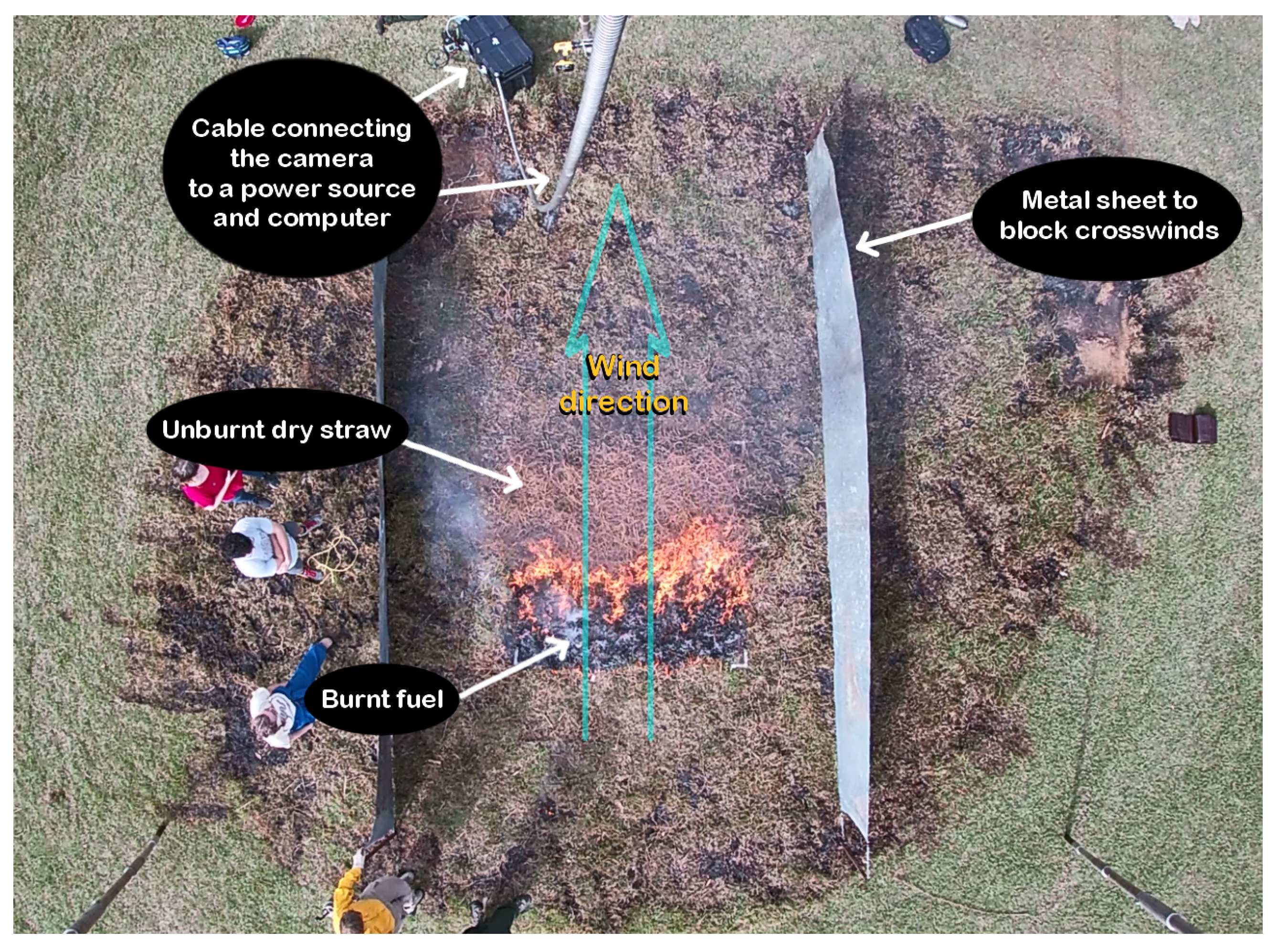
Figure 1.
The experimental setup is a 2 m × 2 m plot of dry pine straw. The setup components are labeled. A fan is used to generate a nearly-uniform wind velocity, and metal sheets eliminate any crosswind effects.
Figure 1.
The experimental setup is a 2 m × 2 m plot of dry pine straw. The setup components are labeled. A fan is used to generate a nearly-uniform wind velocity, and metal sheets eliminate any crosswind effects.

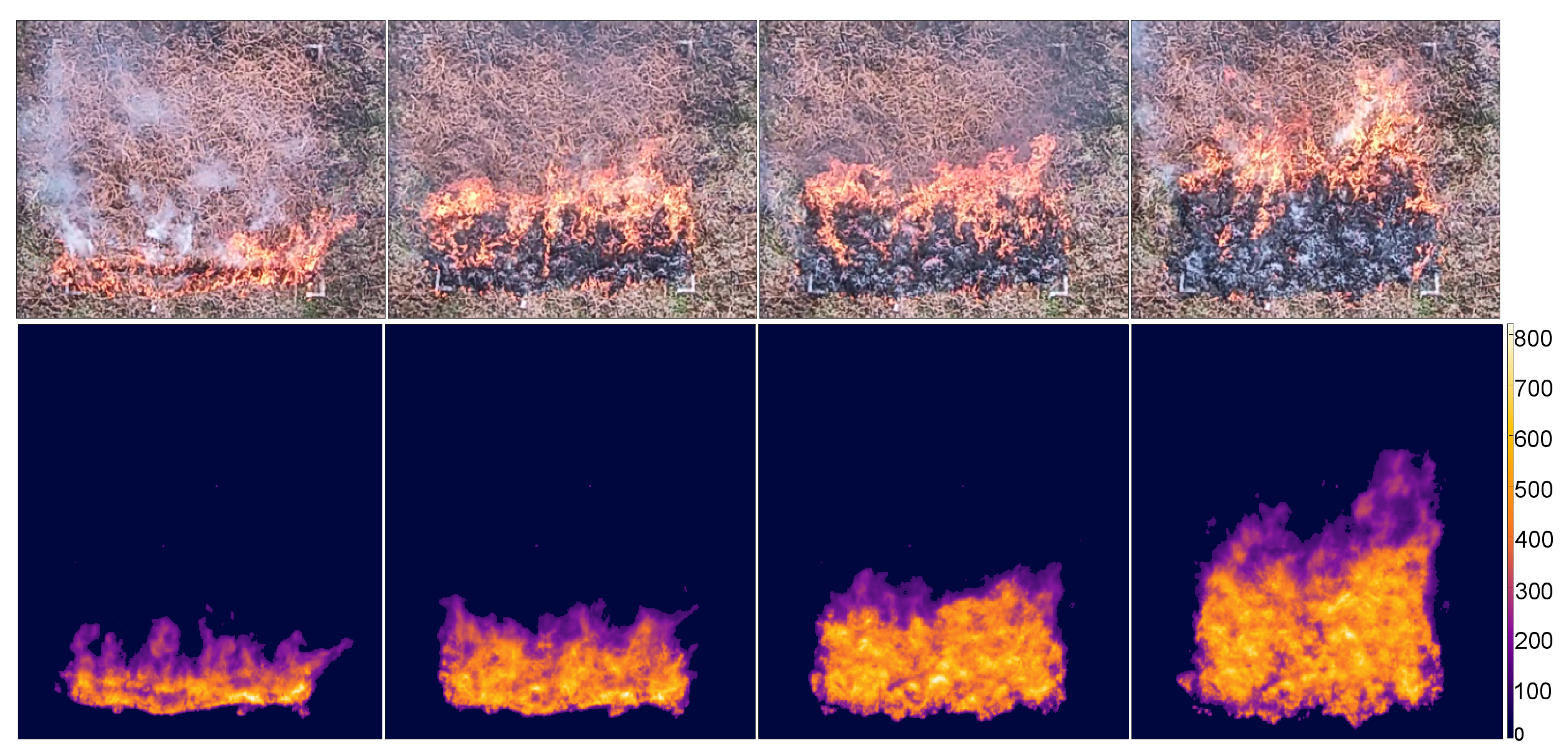
Figure 2.
Visual (top) and infrared (bottom) camera frames at four time steps spaced approximately 10 s apart. The frames of the individual cameras are not perfectly synchronized.
Figure 2.
Visual (top) and infrared (bottom) camera frames at four time steps spaced approximately 10 s apart. The frames of the individual cameras are not perfectly synchronized.

Figure 3.
Sample points found in successive frames used to calculate wind speed along the longitudinal axis. The yellow points yielded a wind speed of approximately m/s, the green points yielded a wind speed of approximately m/s, and the cyan points yielded a wind speed of approximately m/s; combined, the average wind speed in the positive longitudinal direction is m/s.
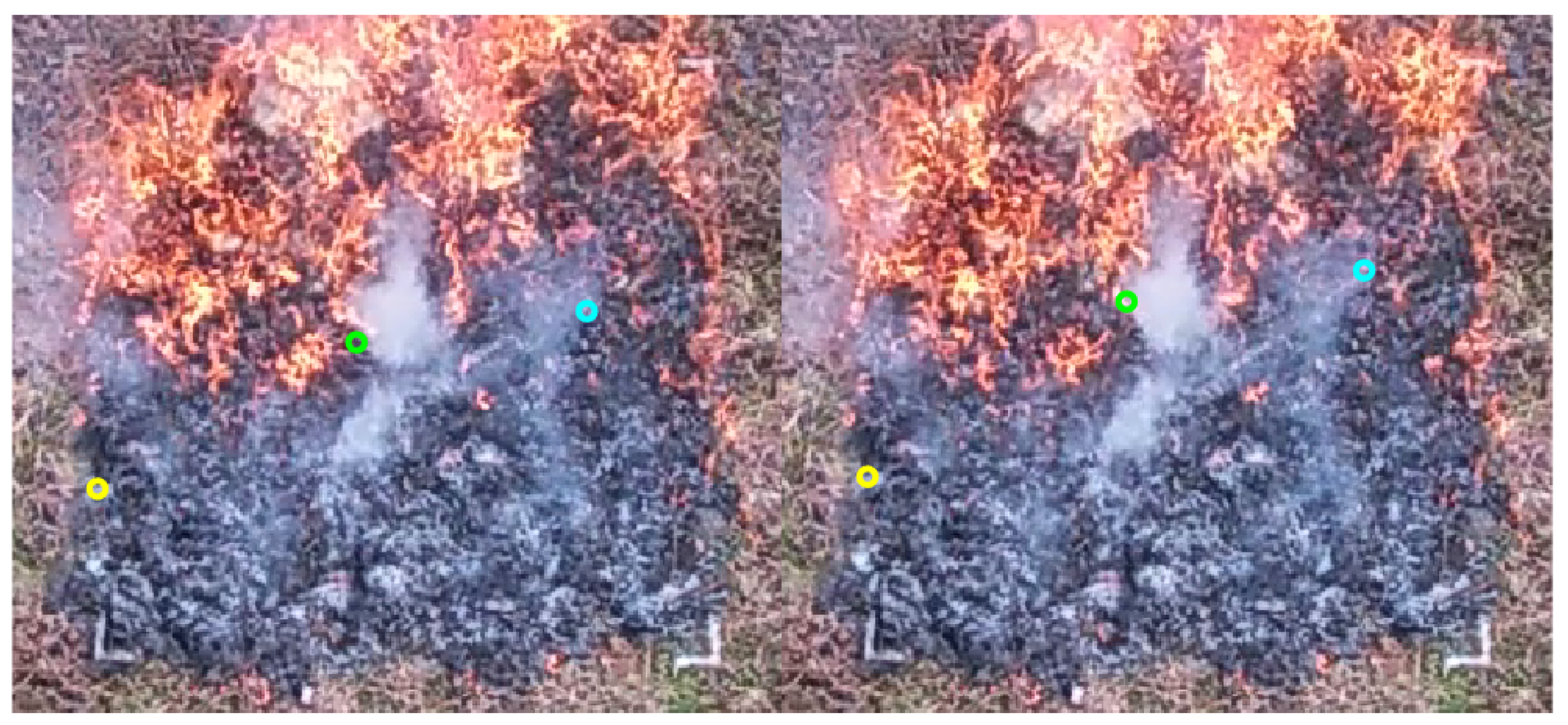
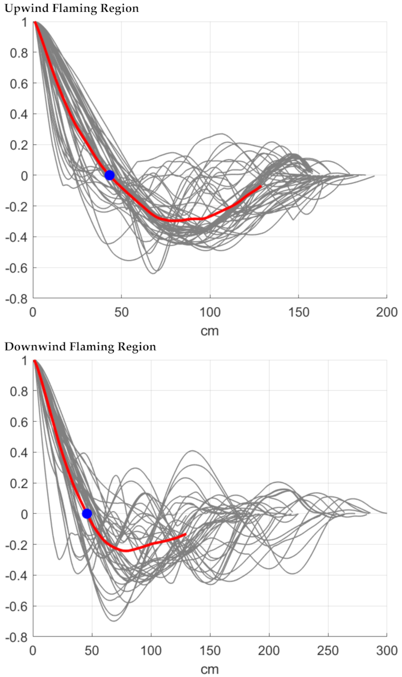
Figure 4.
(Left): A schematic of the experimental setup. The RoS of the upwind side of the flaming region is tracked. (Right): A typical time series of a pixel. The colors coincide with those in Figure 6.
Figure 4.
(Left): A schematic of the experimental setup. The RoS of the upwind side of the flaming region is tracked. (Right): A typical time series of a pixel. The colors coincide with those in Figure 6.
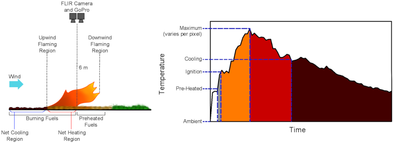
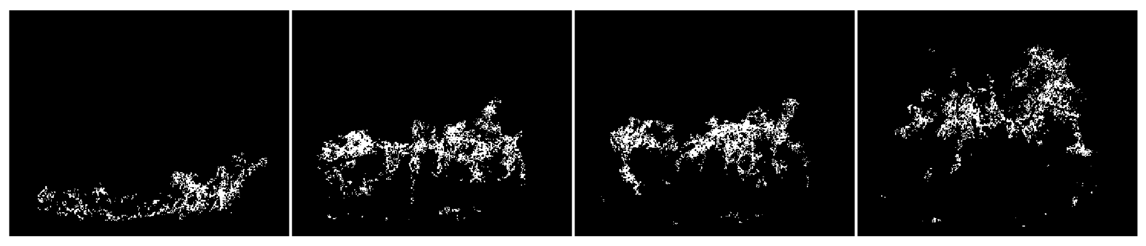
Figure 5.
Regions from the frames in the top row of Figure 2 that are part of the active combustion zone. The RGB value of is sampled from a pixel that is known to be in the combustion region. After experimenting with different tolerances for a single frame, tolerances of 15 (R), 60 (G), and 40 (B) are chosen, and these are used to define actively combusting pixels in every frame.

Figure 6.
Regions from the frames in the bottom row of Figure 2 that are heating (gray), fully combusting (between the ignition and maximum temperature, orange), and cooling (red and dark brown). Fuels in the dark brown region are still undergoing combustion but have cooled below C.
Figure 6.
Regions from the frames in the bottom row of Figure 2 that are heating (gray), fully combusting (between the ignition and maximum temperature, orange), and cooling (red and dark brown). Fuels in the dark brown region are still undergoing combustion but have cooled below C.
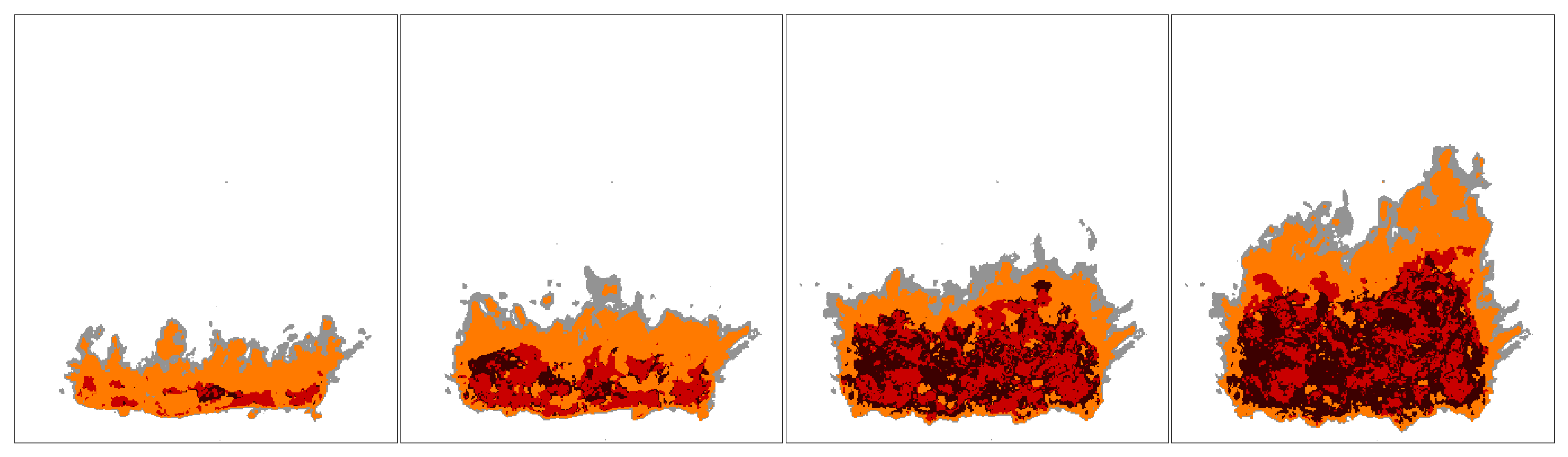
Figure 7.
(Top): Segmented infrared and visual images. (Bottom): Cleaned infrared and visual images.
Figure 7.
(Top): Segmented infrared and visual images. (Bottom): Cleaned infrared and visual images.
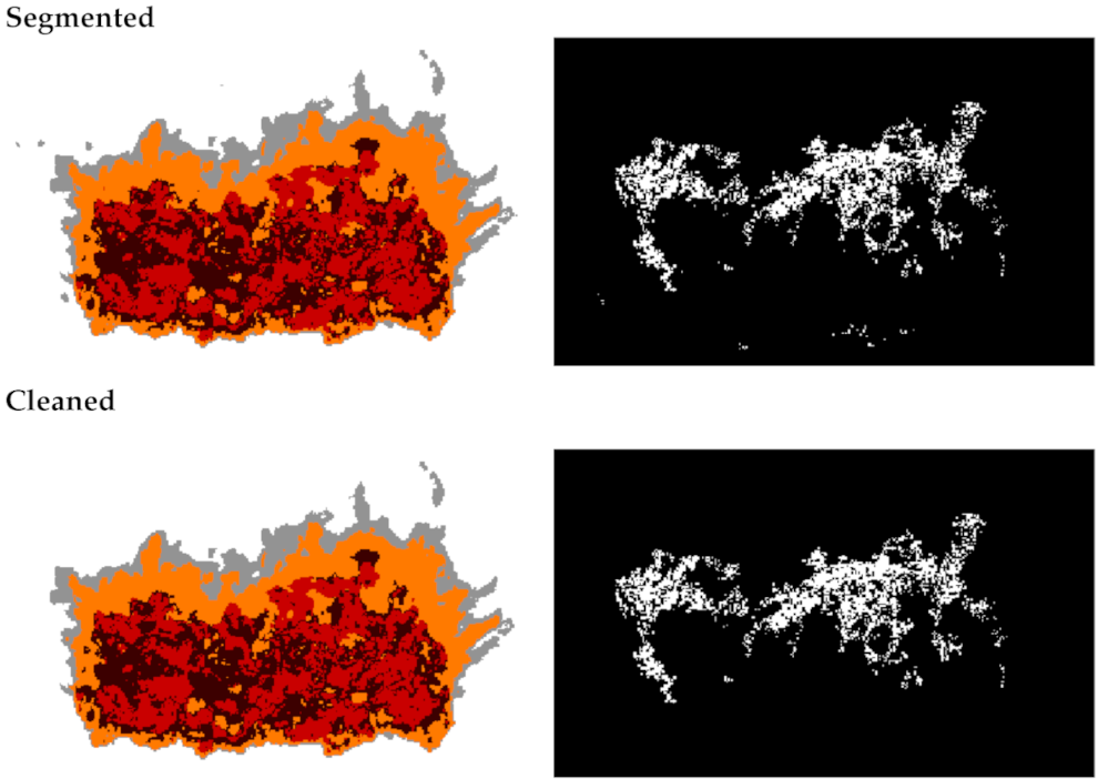
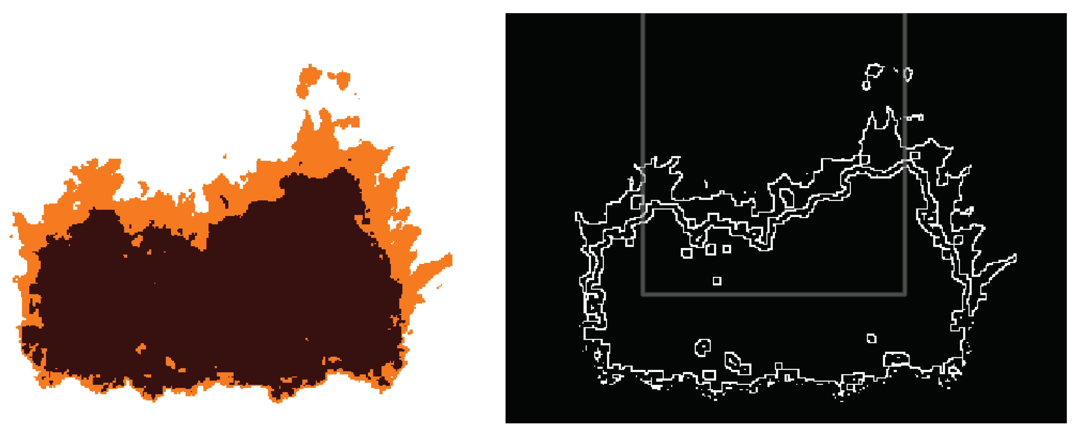
Figure 8.
(Left): Logical mask representing all points determined to be part of the fire system, whether heated, ignited, or burnt. (Right): Edge detection results distinguishing the outline of three regions; heated gas, flame, and burnt area. The isotherm of the upwind side of the flaming region in the gray box is shown in Figure 9.

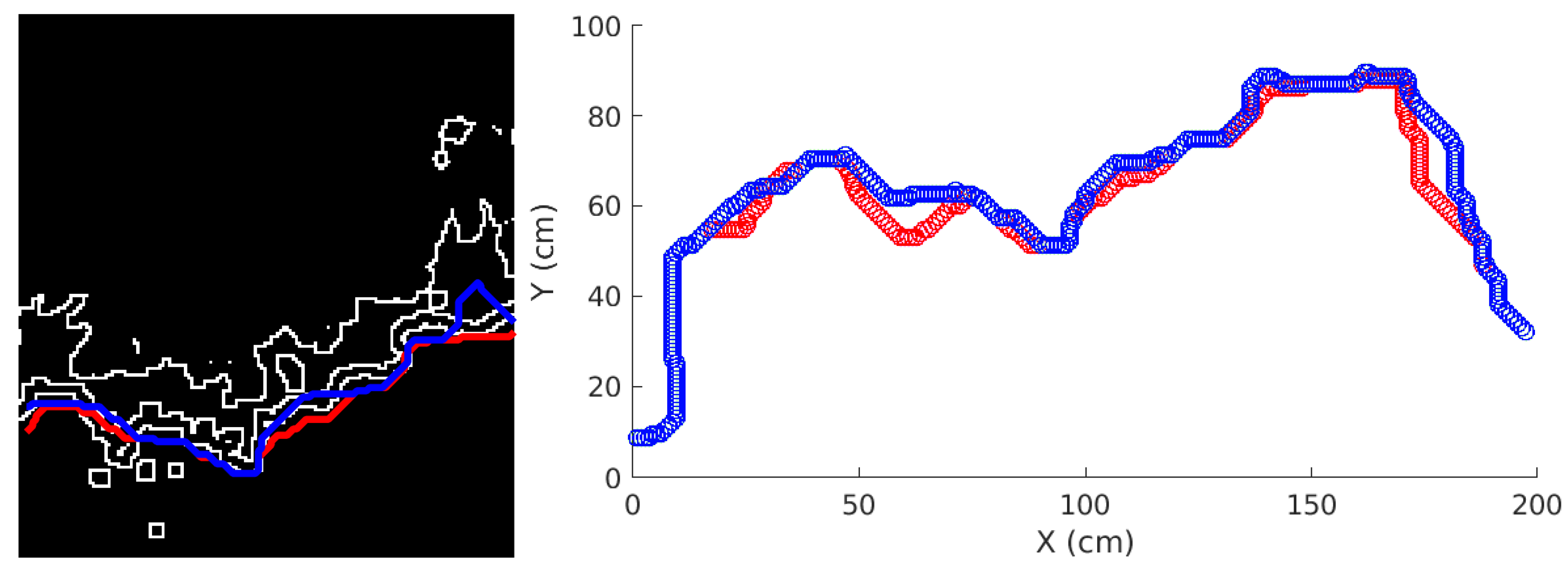
Figure 9.
(Left): Sample Crawler results for frames at successive time steps overlaid on a portion of the middle third of the right plot of Figure 8. (Right): Crawler results for two successive frames converted to coordinates with physical axes. The red and blue points are the result of Crawler at the successive time steps.

Figure 10.
A visualization of the subdomain and buffer zone system applied to Figure 9.
Figure 10.
A visualization of the subdomain and buffer zone system applied to Figure 9.
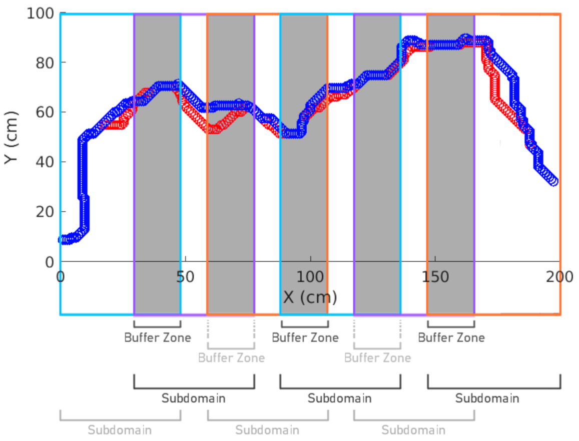
Figure 11.
The mean-shifted autocorrelation of the y coordinate of all isotherms (gray) and their average (red). The chosen length scale is the first root of the autocorrelation function which is about 48 cm for the upwind side and 46 cm for the upwind side.
Figure 11.
The mean-shifted autocorrelation of the y coordinate of all isotherms (gray) and their average (red). The chosen length scale is the first root of the autocorrelation function which is about 48 cm for the upwind side and 46 cm for the upwind side.

Figure 12.
(Top): Displacement vectors using a subdomain length of 10 cm. (Middle): Displacement vectors using a subdomain length of 90 cm. (Bottom): Displacement vectors using a subdomain length of cm as determined in Figure 11. Connections formed with 0 weight points are not plotted.
Figure 12.
(Top): Displacement vectors using a subdomain length of 10 cm. (Middle): Displacement vectors using a subdomain length of 90 cm. (Bottom): Displacement vectors using a subdomain length of cm as determined in Figure 11. Connections formed with 0 weight points are not plotted.
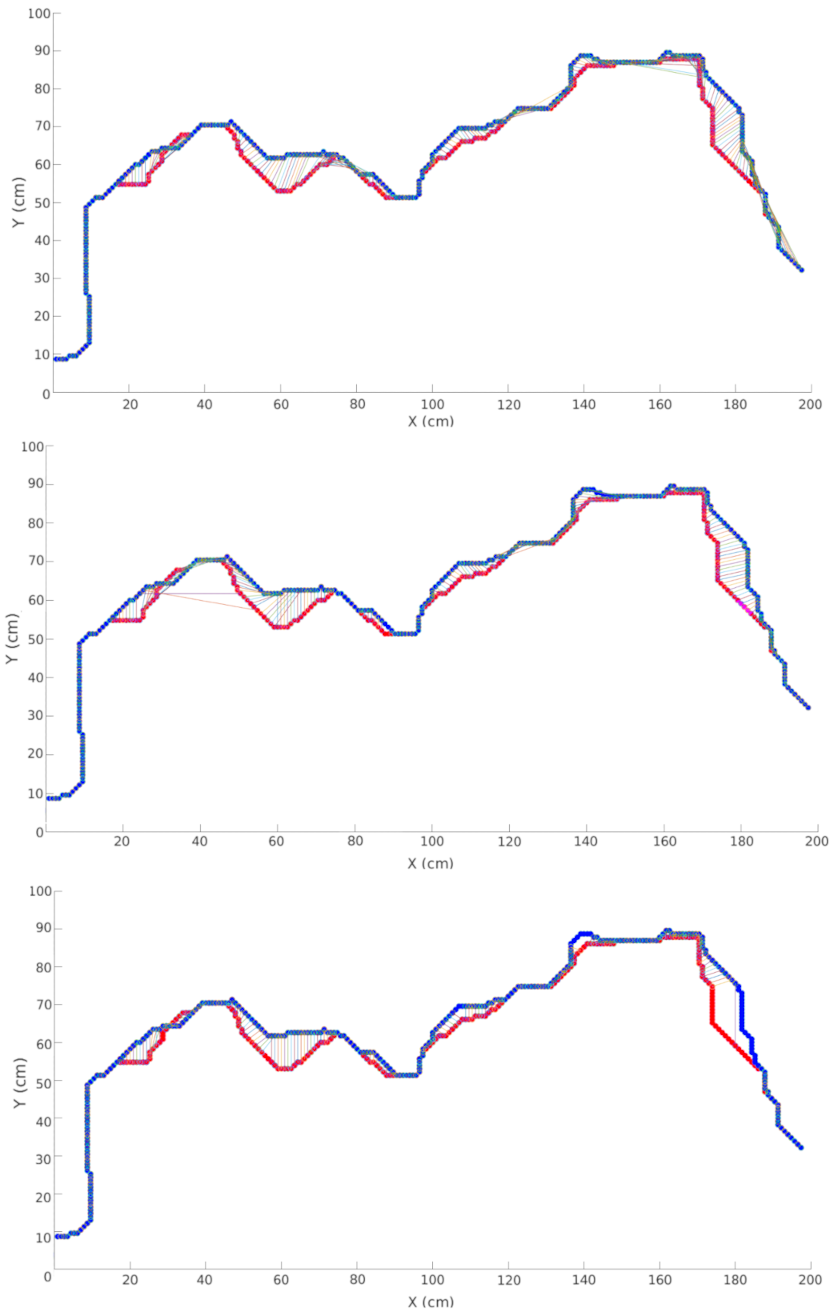
Figure 13.
(Left): Longitudinal velocity distribution with mean cm/s, standard deviation cm/s, and kurtosis . (Right): Transverse velocity distribution with mean cm/s, standard deviation cm/s, and kurtosis . The top plots are in logarithmic scale and the bottom plots are in linear scale.
Figure 13.
(Left): Longitudinal velocity distribution with mean cm/s, standard deviation cm/s, and kurtosis . (Right): Transverse velocity distribution with mean cm/s, standard deviation cm/s, and kurtosis . The top plots are in logarithmic scale and the bottom plots are in linear scale.
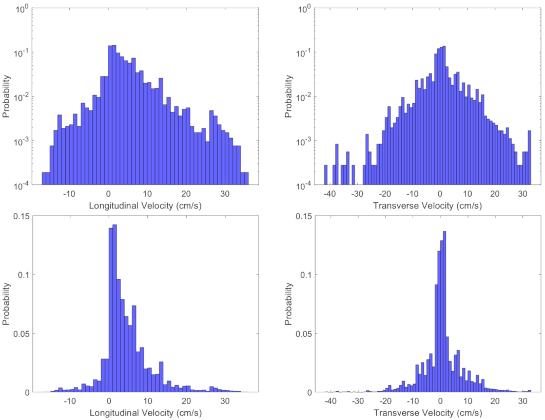
Figure 14.
Positive longitudinal forward RoS distribution in linear scale (left) and log scale (right) with mean cm/s, standard deviation cm/s, and kurtosis . The confidence interval for is . The red curve is an exponential distribution with rate parameter s/cm. The normalized root mean square error between the exponential curve and the data is cm/s.

Figure 15.
(Left): The number of burning pixels, defined using two different ignition temperatures, as a function of time. (Right): The per-pixel time of ignition (first arrival time) of the 2 m × 2 m linear spread plot described in Section 2. The green points correspond to manual ignition positions at time s. The three sets of blue points are isotherms calculated at s (lower), s (middle), and s (upper). Plotted alongside each isotherm are several corresponding velocity vectors.

Figure 16.
(Left): The number of frames each pixel spent between the ignition temperature and the maximum temperature. Since the frame rate is 1 Hz, the color also represents the number of seconds each cell spends burning. (Right): The burn time distribution with mean s, standard deviation s, and kurtosis . The red curve is an Erlang distribution with shape parameter and rate parameter . The normalized root mean square error between the points on the Erlang distribution curve and the data is s.

Publisher’s Note: MDPI stays neutral with regard to jurisdictional claims in published maps and institutional affiliations. |
© 2021 by the authors. Licensee MDPI, Basel, Switzerland. This article is an open access article distributed under the terms and conditions of the Creative Commons Attribution (CC BY) license (https://creativecommons.org/licenses/by/4.0/).
Share and Cite
MDPI and ACS Style
Sagel, D.; Speer, K.; Pokswinski, S.; Quaife, B. Fine-Scale Fire Spread in Pine Straw. Fire 2021, 4, 69. https://0-doi-org.brum.beds.ac.uk/10.3390/fire4040069
AMA Style
Sagel D, Speer K, Pokswinski S, Quaife B. Fine-Scale Fire Spread in Pine Straw. Fire. 2021; 4(4):69. https://0-doi-org.brum.beds.ac.uk/10.3390/fire4040069
Chicago/Turabian StyleSagel, Daryn, Kevin Speer, Scott Pokswinski, and Bryan Quaife. 2021. "Fine-Scale Fire Spread in Pine Straw" Fire 4, no. 4: 69. https://0-doi-org.brum.beds.ac.uk/10.3390/fire4040069