
A Deep Learning Based Object Identification System for Forest Fire Detection
by
 , , , and
Federico Guede-Fernández
1,2,3,† ,
,
Leonardo Martins
1,2,† ,
,
Rui Valente de Almeida
1,2,† ,
,
Hugo Gamboa
1,3 and
and
Pedro Vieira
1,2,*
1
Physics Department, NOVA School of Science and Technology (Campus de Caparica), 2829-516 Caparica, Portugal
2
Future Compta SA, 11495-190 Alges, Portugal
3
LIBPhys (Laboratory for Instrumentation, Biomedical Engineering and Radiation Physics), NOVA School of Science and Technology (Campus de Caparica), 2829-516 Caparica, Portugal
*
Author to whom correspondence should be addressed.
†
These authors contributed equally to this work.
Fire 2021, 4(4), 75; https://0-doi-org.brum.beds.ac.uk/10.3390/fire4040075
Submission received: 7 September 2021
/
Revised: 1 October 2021
/
Accepted: 11 October 2021
/
Published: 17 October 2021
(This article belongs to the Section Fire Science Models, Remote Sensing, and Data)
Abstract
:Forest fires are still a large concern in several countries due to the social, environmental and economic damages caused. This paper aims to show the design and validation of a proposed system for the classification of smoke columns with object detection and a deep learning-based approach. This approach is able to detect smoke columns visible below or above the horizon. During the dataset labelling, the smoke object was divided into three different classes, depending on its distance to the horizon, a cloud object was also added, along with images without annotations. A comparison between the use of RetinaNet and Faster R-CNN was also performed. Using an independent test set, an F1-score around 80%, a G-mean around 80% and a detection rate around 90% were achieved by the two best models: both were trained with the dataset labelled with three different smoke classes and with augmentation; Faster R-CNNN was the model architecture, re-trained during the same iterations but following different learning rate schedules. Finally, these models were tested in 24 smoke sequences of the public HPWREN dataset, with 6.3 min as the average time elapsed from the start of the fire compared to the first detection of a smoke column.
1. Introduction
Forest fires have been one of the most devastating events in recent years, due to their uncontrollable nature, with a 2002–2016 mean annual global estimated burned area of 4,225,000 km² [1]. Human activities are accountable for over 90 (per cent) of wildland fires, with sudden lightning discharges accountable for most of the remaining fires [2], as controlled fires are still used to manage and shape the Earth’s landscapes and ecosystems. In most of the developed countries, human activities that involve the use of fire are highly regulated by several laws and are normally policed by government agencies [3]. There have been recent movements that advocate for limiting, even more, the use of controlled fires, as they have been linked to ecological and health damages, such as the link to the increase in Tropospheric ozone level or increased inhalation of smoke particles [4,5,6,7]. While the use of controlled fires has been found to have benefits to some plants and animal species, it has also been found to leave irreparable damage to the other species [8].
Applications related to the prediction, management and detection of wildfires have been improved in recent years with the use of Machine Learning methods [2]. A recent study [3] has shown that investments in detection innovations, such as fire weather services, fixed lookouts and geospatial technologies can achieve high net benefits in the medium or long term, when considering that they have a high cost investment at short term (due to the services installations), but can provide savings for each fire that was controlled at an early stage, with most of the developed system with systems ranging from signal-based to image-based [9,10,11].
The main difference between these detection systems is based on their strategic approach leading to their categorization into three main groups: wireless network sensing, satellite monitoring techniques and large-area remote sensing. The wireless network sensing approach is normally based on local devices patrolling the target region and rely on the communication capabilities between a large number of sensors (e.g., temperature, humidity and luminance) [9,12]. Their biggest drawbacks are their very limited restricted range of operation, their low lifetime and environmental issues with malfunction systems [9]. The satellite monitoring techniques such as MODIS (MODerate resolution Imaging Spectroradiometer) and AVHRR (Advanced Very High Resolution Radiometer) sensor scanners were deployed respectively in the Aqua/Terra and NOAA satellites and have been extensively used for earth monitoring activities [13]. Their biggest drawbacks are their low temporal and spatial resolutions [14]. Examples of this are the SmokeNet platform, which uses MODIS information to classify six classes of images (i.e., cloud, dust, haze, land, seaside, and smoke) [15] and a framework based on Inception-v3 a convolutional neural network architecture developed by GoogleNet [16], which detects fire and non-fire images from satellite images [17]. The large-area remote sensing system is usually based on an automated warning system based on optical principles (e.g., cameras or spectrometers) in order to detect smoke plumes or flames at large distances, whether optical cameras or [11]. Most of these types of networks quickly evolved into commercial systems, such as the FireWatch and ForestWatch [18]. This is the type of system (fixed lookout) that has been evolving in our research work [19,20].
The main objective of this research work is to present a fixed lookout system that is able to acquire real-time images, that can then be processed by deep learning algorithms in order to perform object detection tasks, using the Detectron2 platform. This system is able to detect smoke plumes over large areas can be able to communicate and warn the authorities of fires in the early stages, which can prevent the escalation of wildfires.
2. State of the Art
Some of the above-mentioned systems have been using traditional detection methods since their first implementation, but the use of Machine Learning techniques has started to capture more interest in recent years, with Deep Learning techniques gaining traction in the last two years, as one of the main tools used in the automatic recognition of forest fires [2,11]. The most common models that are implemented for smoke and fire detection and classification in images are based on either CNN (Convolutional Neural Networks) [15,21], Faster R-CNN [21], Fully Convolutional Neural networks [22] or Spatio-spectral Deep Neural Networks [23]. Some of the most recent studies in fire detection systems have also been changing their traditional Deep learning approaches to object-based detection systems [24,25], which has also been rising in popularity in the Industry.
The use of object-based detection algorithms has been recently and extensively reviewed [26], which separated the initial algorithms, stemming from the Viola-Jones Detectors, from the main current research lines which can be split into two large group, as also mentioned in this review of the latest advances in the area [27]. The division is based on the number of stages, as the ones based on one-stage detectors are normally associated with the You Only Look Once (YOLO) algorithm [28] and its newer versions (v2 to 4) [29,30,31] and similar alternatives such as the Single Shot MultiBox Detector (SSD) [32]. One of the main identified problems with single-stage detectors was the large class imbalance between foreground and background boxes, which prompted the development of the RetinaNet algorithm which uses focal loss to improve the prediction accuracy, as the estimated loss added to the algorithm is lower if the box is identified as background and higher if it is counted as foreground [33].
The main characteristic of single-stage detectors is that the detection of the bounding boxes and the object classification task is done by the same single feed-forward fully convolutional network. One of the main examples of this type of network is the Feature Pyramid Network (FPN), which is used by RetinaNet but also by two-stage detectors such as the Faster R-CNN, and is able to generate and crop Region-of-Interest (RoI) features maps which are then selected in the most proper scale to extract the feature patches based on the size of the RoI [34].
On the other hand, two-stage detectors, especially the ones that originate from the Region-Based Convolutional Neural Networks (R-CNN) family, as initially proposed by Ross Girshick [35], have the same initial step as the single-stage of compilation of bounding boxes succeeded by a feature extraction method, but are then followed by a final class prediction step, based on which extracted features [27]. Most of these steps are considerably slow, which prompted the development of modified versions that are able to accelerate the first step, such as the so-called Fast R-CNN model proposed in [36], which uses pre-trained images from a classification backbone model such as ResNet [37] and VGG-16 [38] to extract the features with a faster efficiency. The Fast R-CNN algorithm, uses a selective search algorithm to find out the region proposal which is a slow process and becomes the bottleneck of the object detection architecture, which was later upgraded with a version called Faster R-CNN and used a Region Proposal Network (RPN) to detect objects regions from the multi-scale features and incorporate the region proposal in the final step (which is trained simultaneously with the label classification step), revamping the time and accuracy of the objection detection task. The final task is completed by the RoI head which crops and wraps feature maps using proposal boxes into multiple fixed-size features and obtains fined-tuned box locations and scores via the fully connected layers, which are then checked for overlap using non-maximum suppression.
In terms of particular cases of fire detection based on remote imaging sensing systems and applying CNNs for object detection tasks, we identified two types of recent studies, the first ones classify examples of visible fire from very close distances, such as [39,40,41,42], while the second ones try to detect both fire and smoke columns visible in larger distances [43,44].
The majority of the previously developed image processing platforms have been tailored to specific sets of images, since designing an algorithm that could achieve high specificity and sensitivity for an extensive range of cases is still one of the biggest challenges in Image Processing [45]. Due to this situation, it is important to use benchmark datasets, which are normally created by independent organisations and have been manually curated by experts, or online databases created in Contests and Open Challenges [45]. One such database is the HPWREN Fire Ignition images Library, curated by two groups from the University of California San Diego and provided several examples from the remote part of Southern California [46].
3. Data and Methods
3.1. Dataset
The dataset is composed of forest images that were taken with the same acquisition system as in our previous work [20]. The acquisition system is based on a pan and tilt optical camera which is controlled remotely by a server. A bi-spectrum temperature measurement pan and tilt camera IQinVision IQeye 7 Series (IQ762WI-V6) was used for image acquisition. The images were taken with the visible camera of this device which has the following specifications: image sensor of 1/3" CMOS sensor, an effective resolution of 1080p, and a 12–40 mm telephoto lens with an 18° wide and 9° tele-oscillatory ventilation.
The images were acquired during daylight and the azimuth of the camera changed at a pre-defined position using a fixed time rate in order to span the 360° of the horizon. The acquisition of the dataset was done in ten different systems located in the Peneda-Gerês National Park in Portugal.
The labelling process was performed with the OpenLabeler platform [47] to annotate the visible objects by defining a bounding box area where the object is located and tag it with a name, this information is saved in the PASCAL VOC XML format. These annotations can then be converted into a JSON file in COCO format which is processed by the Detectron2 [48].
The initial labelling of the images was done with the smoke label but after some tests, it was decided to define three subclasses of smoke objects namely: hrz, mid and low, as this sub-categorisation, allows for more detailed information of smoke columns and also accounts for a large variation in visual appearances. This sub-categorisation was done subjectively, based on the distance between the base of the smoke column and its distance to the horizon and the camera. The first ones, hrz are comprised mostly of smoke columns above the horizon such as smokes, with the base of the smoke starting at the top of the mountain or with a base of the smoke column not visible since it starts at the non-visible side of the mountain. These smoke columns tend to extend fast into the sky and over the horizon and can be mistaken by clouds due to their high position. The second ones, mid, are characterised by smoke columns that have a base present predominantly at the middle of the image (vertical-wise). While the smoke column can extend over the horizon, their body has a significant background of land. The last type of smoke columns, low, consist of smoke columns that start close to the acquisition camera, as these can occupy a large part of the image and the base of the smoke is normally not visible since the distance to the camera might cut the base from the picture. The size of these smoke columns (in terms of pixels) also grows very large in a shorter amount of time, due to the distance to the camera. Examples of these three types of smoke objects are shown in Figure 1.
During the first model training sessions with the smoke class and the three classes (hrz, mid and low), some clouds were wrongly detected as smoke objects. Then, images containing clouds but not smoke were labelled as clouds and included in the dataset. Moreover, it was detected that some images without annotation labels of either smoke or cloud were being wrongly detected as a smoke object. One of the strategies to overcome this problem is to introduce it into the dataset as an input image without any smoke or cloud annotation, similarly to the strategy reported in [49], where they found that the addition of images without any annotation to the dataset may lead to decrease the number of false detection’s [49]. These images are characterised to be similar to other forest images but there is no presence of smoke or cloud so they do not have any annotation and they are referred to in this paper as empty samples.
Image augmentation techniques were also used, based on the Albumentations library [50], (which has a widespread usage in deep learning and has been licensed under the MIT license). Image augmentation allows the creation of additional training examples, without the time-consuming task of manual labelling, using as a base the existing images. The initial number of images was doubled using this library, based on three different augmentation techniques, namely: Horizontal Flip (with a 0.25 probability for each image), Rotation (with a limit of 15 and a probability of 0.5), and finally an RGB Shift (with a limit of 15 for each colour and a probability of 0.5). These augmentations processes allow the system to be more robust to the introduction of new conditions such as different lighting coming from the sun, or different directions of smoke columns.
The characteristics of the dataset which was used in the training and validation phases are shown in Table 1. The version name specifies the characteristics of the dataset, the number denotes the classes cardinality, whether it was labelled using only the class smoke (1) or if it was labelled with hrz, mid, low classes (3). The letter “A” denotes if the augmented images were added to the dataset, the letter “C” means that images that were labelled with clouds were added to the dataset and the letter “E” indicates if empty images (without any annotation) were included in the dataset. In Table 1, the columns hrz, mid and low indicate the number of the smoke images which are labelled as hrz, mid and low respectively, so it has not been added new images. It must be remarked that for one row, the sum of hrz, mid and low is not equal to the smoke images due to some images being labelled as hrz, mid or low in different regions. Therefore, these columns specify the number of images that have been labelled as hrz, mid or low. Furthermore, the number of images of smoke, clouds and empty was balanced but during the creation of the (hrz, mid and low), it was not possible to balance these three types of objects, due to the lower presence of hrz and low compared to mid fire objects.
Two different datasets were used: one for the training and validation phase and the other for testing the model. The first dataset was randomly partitioned into training and validation images with 80% and 20% proportions respectively. The dataset which was used for testing is compound by images that were not used in training or validation. It contains a total number of 375 images with smokes, 1249 with clouds and 2021 empty images. These smoke images are grouped in 75 sets of 5 images which correspond to the first 5 images that were taken at a determined location since the beginning of the smoke. Due to the setup characteristics, the mean time elapsed between each image is 380 s ± 120 s, so the testing dataset contains 75 sequences of different smokes originated at different locations to assess the classification performance of the smoke detection algorithm at different smoke stages.
3.2. Architecture of Object Detection Models and Transfer-Learning
The Detectron2 is an open-source object detection framework that has been developed by Facebook AI Research and is implemented in Pytorch. This framework can be used to train various state-of-the-art models for detection tasks such as bounding-box detection. In this paper, this framework has been used to build the smoke detection model based on a two-stage object detection architecture that outperforms single-stage detectors in terms of accuracy.
Detectron2 has available the Faster Region-based Convolutional Neural Network (R-CNN) model with Feature Pyramid Network (FPN) backbone which is a multi-scale detector that achieves high accuracy in tiny to large object detection tasks [34]. The Detectron2 has been used to train with our dataset a model based on the Faster R-CNN architecture which was pre-trained on ImageNet.
Both the adopted models (RetinaNet and Faster R-CNN) were available from the Detectron2 Model Zoo [51]. Their architectures are composed by the ResNet with 50 layers as backbone combined with the Feature Pyramidal Network. The weights of models were initialised with their pre-trained architecture on the MS COCO dataset using the full learning rate schedule (3x, ∼37 COCO epochs).
The RetinaNet and Faster R-CNN models were then re-trained for smoke classification with specific parameters and datasets. The learning rate scheduler and the number of iterations of the re-trained process were varied to evaluate the classification performance of these parameters. The number of iterations were 3500 and 5000 which were chosen empirically and the learning rate strategies were the warm-up constant (WUP) learning rate of 0.001 and a triangular cyclical (CYC) learning rate with a maximum learning rate of 0.01 and a base learning rate of 0.005. The WUP is a simple and commonly used learning rate strategy while the CYC learning rate is a more sophisticated strategy that could improve the classification accuracy without a need to tune [52]. Then, the RetinaNet was re-trained with warm-ump learning and with 3500 and 5000 iterations which were called RetinaNet_3500_WUP and RetinaNet_5000_WUP respectively. The Faster R-CNN was re-trained for 5000 following WUP and CYC learning rate scheduler, they were called FRCNN_5000_WUP and FRCNN_5000_CYC respectively. Moreover, these four models were re-trained separately over the 16 datasets described in Table 1, so 64 different models were finally re-trained.
These experiments, which were conducted to train and test the object detection based models, were all performed on a computer configured as follows: the CPU was an Intel i7 9700k at 3.6 GHz with 8 cores, the graphics card was a dual NVIDIA RTX2080, the RAM memory was 64 GB and a hard disk of 2 TB. The software environment was as follows: the operating system was Ubuntu 18.0.5, the programming language was Python 3.8.5 and the main Python software libraries were: pytorch (v.1.7.1), torchvision (v. 0.8.2), opencv-ptyhon (v. 4.4.0.46), Detectron2 (v. 0.3), albumentations (v. 0.5.2) and numpy (v. 1.19.2).
3.3. Performance Evaluation
The intersection over union (IoU) metric is commonly used for the evaluation of object detection algorithms. The IoU, which is also known as the Jaccard index, calculates the ratio of the intersection area of the bounding boxes over the area of the union of the bounding boxes as defined in Equation (1):
The IoU determines the overlap between the predicted bounding boxes and the ground-truth bounding boxes from the labelled dataset. Therefore, the predicted bounding boxes that highly overlap with the ground-truth bounding boxes have higher scores than those with lower overlap. The IoU can then be used to determine if the object detected by the model is true or false, by setting the IoU to a fixed threshold in order to determine the correctness of the detection. If the IoU is higher than the specified threshold the detection is considered to be correct, otherwise it is discarded [48].
The average precision (AP), which is based on the IoU, is a popular metric in measuring the accuracy of object detection algorithms. The general definition for AP is the area under the precision-recall curve. The calculation of the AP is based on an interpolation of 10 points, which is the average over multiple IoU and with each IoU being used as the minimum IoU to consider a positive match. In the presence of more than one class in the dataset, the AP is computed as the mean for each class. Therefore, AP is used to show the detection performance of the smoke detection model for all classes. Particularly, the AP metric corresponds to the average AP for IoU from 0.5 to 0.95 with a step size of 0.05, as is expressed in Equation (2):
To test the performance of the deep learning-based model for smoke detection, the following metrics were computed:
- True positives (TP) is the number of images which was detected as smoke correctly, it is determined by an IoU is greater than 0.33.
- False positives (FP) is the number of images that were badly detected as smoke, it is determined by an IoU lower than 0.33.
- False negatives (FN) is the number of images that were not detected as smoke incorrectly.
An IoU score greater than 0.5 is normally considered a good prediction but 0.33 was chosen as the smoke object can have a fuzzy appearance, so the intersection of both bounding boxes was lowered in order to keep positive smoke detections that would be otherwise discarded.
The F1-score metric (obtained from the aforementioned TP, FP and FN) was used to evaluate the classification performance in validation and testing. The precision quantifies the number of the smoke detections that actually belong to the smoke class while recall computes the number of smoke detections of all images labelled as smoke. In addition, F1-score is a single indicator that balances both the precision and the recall, as defined in Equation (3):
Moreover, other metrics were calculated to evaluate the ratio of false detection of the model for images labelled with clouds or without annotations but which are wrong classified as smoke, as defined for the following examples:
- The true negatives (TNc) is the number of images annotated as clouds that were not classified as smoke
- The true negatives (TNe) is the number of images without annotations that were not classified as smoke.
- The false positives (FPc) is the number of images annotated as clouds which were classified as smoke
- The false positives (FPe) is the number of images without annotations that were classified as smoke.
The false detection rates FPRc and FPRe were also used to evaluate the wrong classifications of cloud objects and of empty images respectively (no annotation). These metrics are defined in Equations (4) and (5):
Additionally, the G-mean quality metric was also calculated, which can be applied in imbalanced datasets. This performance metric evaluates the true detections and the false detections for smoke, clouds and empty annotations jointly by micro-averaging the specificity for the samples of three classes: smoke, cloud and empty. The micro-averaging was performed by weighting each sample equally to compute the average metric. The TPT, FNT and FPT were defined as the sum of true positives, false negatives and false positives respectively for the smoke images located from the beginning of the smoke until the image of the fifth position. The false-positive rate (FPRT) denotes the number of images wrongly detected as smoke over the total number of images without any smoke annotation. The metrics are expressed in Equations (6)–(9):
Finally, the detection rate (DTR) metric was defined to assess the smokes detection performance over the time-sequenced smoke images. The DRTn is the percentage of sequences that have at least one true smoke detection in the n first images over the total number of sequences (75).
4. Results and Discussion
4.1. Test Set with Smoke, Clouds and Empty Images
Table 2 shows the classification performance metrics for the specifically employed model architectures which were trained with different parameters as described in Section 3.2. It should be noted that for each architecture, the two initial rows show the configurations with the best results, following the maximization of the G-mean criteria. In contrast, the third row shows the worst model obtained in order to illustrate the difference associated to use different dataset configurations for the same pre-trained model. The F1i denotes the F1-score of the smoke image at the position ith of the fire sequence and the FPRC, FPRE and FPRT denote the false-positive ratio for cloud, empty and all images respectively. Finally, G-mean is shown as a quality indicator that balances the detection rate of smoke and non-smoke images.
The Table 2 reveals that the inclusion of empty samples improves the FPR for empty images and it seems to have a positive impact on smoke detection. The addition of cloud samples improves the FPR for cloud images in most cases but it is not clear their negative impact on smoke detection. The FPRT for all the images follows a similar trend to the other two False Positive rates, with the best-case scenario having an FPR value of around 5%.
Moreover, the best F1-score results are achieved in the fourth image for the models FRCNN_5000_WUP, FRCNN_5000_CYC and RetinaNet_3500_WUP but it can be achieved in the fourth or fifth image for RetinaNet_5000_WUP. Temporal evolution of the F1-score is shown in this Table, a positive trend in the evolution can be appreciated for the different models between F11 and F14 but the direction of trend change between F14 and F15 for almost all cases.
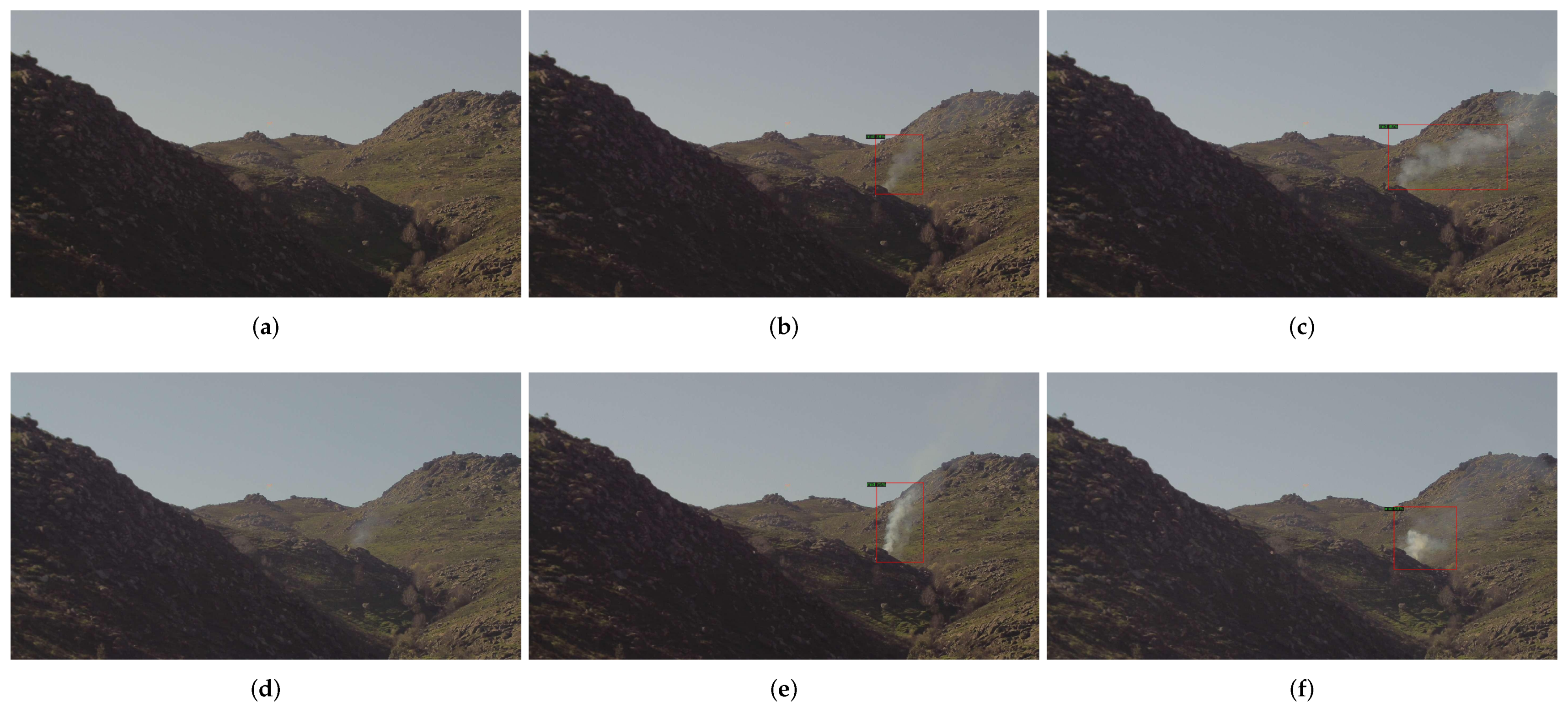
The results obtained for the two best models of both FRCNN_5000_WUP and FRCNN_5000_CYC are quite similar but the FRCNN_5000_CYC with the dataset 3AE can be considered as the preferable model due to the best performance in terms of G-mean, it shows the best overall F1 score and also the results of F1-scores are better for the images located in the three first time positions. Figure 2 shows a sequence of six time-consecutive images taken in the same fixed position.
4.2. Temporal Evolution of Smoke Detection Rate
Table 3 shows the accumulated true detection rate of images annotated with smoke over time. This indicator assesses the ability of the trained model to detect smoke at least in the first images since the smoke starts in the test set. This table shows the results of the same models as those shown in Table 2. The temporal evolution shows that FRCNN_5000_CYC achieves a result of over 80% in the DTR3, which is remarkably better than the other models and for DTR5 it is slightly better than the best of FRCNN_5000_WUP. In addition, the impact of the training with a different dataset for the same architecture is observed due to the large difference observed between the worst model of each architecture and the two best models that are shown in Table 3. As it can be expected, the models with higher F1 scores also have a high DTR percentage and they also achieve a better overall result in the last image.
4.3. Average Precision in Validation Set
Table 4 shows the average precision (AP) performance metric of the models selected based on the same aforementioned criteria. The AP50 and the AP75 represent the AP obtained using the IoU with a threshold of 0.50 and 0.75 respectively and computed in the validation set.
As it was previously referred to in the literature, both RetinaNet based models achieved better results in terms of AP than the Faster R-CNN models. However, these results can be caused by the nature of the datasets 1A and 1 without the presence of clouds or empty images. It must be noted that the difference for the same dataset (3CE) between RetinaNet_5000_WUP and FRCNN_5000_WUP is not such great as RetinaNet_5000_WUP 1A an FRCNN_5000_WUP 3AE. Moreover, the comparison of AP between models for the same architecture must be taken with caution because they are obtained with different datasets.
The difference between the AP50 and AP75 values can be attributed to the fact that although when the object is detected, it might not match totally with the region defined by the labels. As the main objective of the final application of this model is to detect the smoke to generate alarms, these differences are not a major issue as long as a high AP50 value can be obtained.
4.4. Comparison with HPWREN Public Database
This section shows the results of the implemented method using the HPWREN dataset [46]. This dataset has been selected to obtain comparable results since it contains images of fires originating in non-urban areas with a temporal sequence of images before and after the fire ignition and the images are publicly available. This dataset was acquired in areas of southern California, that may have different environments to the ones trained by our system, although both were acquired from a high-ground position, allowing the visibility of both ground areas and the skyline.
Moreover, a previous work, which also uses an object detection model based on deep learning, provides the time elapsed from the fire starts until their model detects the fire for sequences of the entire dataset [43]. It must be remarked that the videos are composed have a frame rate of one image per minute. The names of the first eight video sequences are the same as those mentioned [43], with one more smoke sequence that is not currently available in the HPWREN database. In addition, 16 more sequences present in the HPWREN database have been added to this study, which were not available at the time of the previous publication [43].
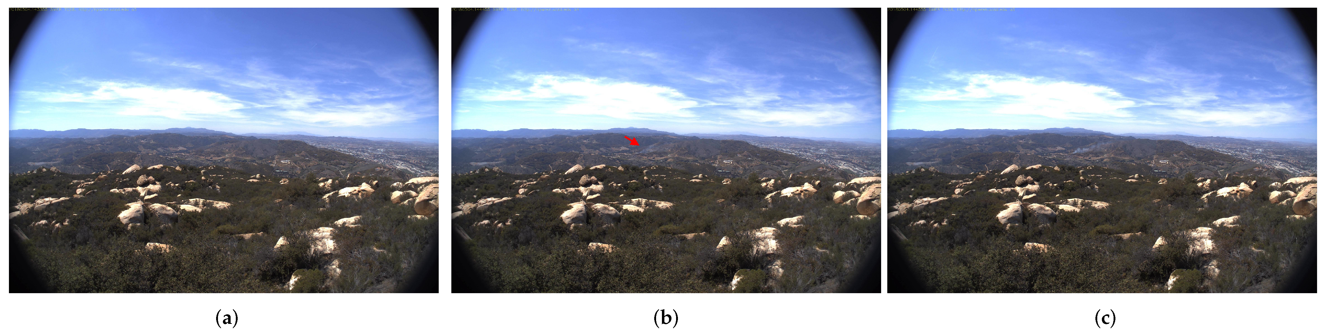
The reference time of the start of the fire was provided [43] for the 8 first sequences but for the other 16 sequences, the reference fire start time was defined by us, because the smoke is not visible in the image frame associated with the time provided in the filename of the sequence. Figure 3 shows a sequence with the reference provided by the filename and the fire start time defined by us.
Table 5 shows the time elapsed from the fire ignition, from the time detected for the first time with the reference method, our two best models (FRCNN_5000_CYC with 3AE and FRCNN_5000_WUP with 3AE), and the worst one (RetinaNet_3500_WUP with 1CE). The first column shows the name of the video sequence as mentioned [43] for the eight initial sequences and the identification name in the HPWREN database directory for the other 16 sequences that were also added. The penultimate row of the table shows the calculated times for the initial eight sequences for comparative purposes with the reference method, while the last row shows the mean time-averaged for the 24 sequences. The obtained results with the proposed model FRCNN_5000_WUP with 3AE are relatively better than those obtained with [43] for the reference 8 images, obtaining a mean detection of over two minutes faster (it is noted, that our model has a much larger standard deviation, due to the late detection on the DeLuz Fire example and the very early detection on the Holy Fire South View example). The model FRCNN_5000_WUP with 3AE detects the smoke fire 1.5 min earlier than FRCNN_5000_CYC with 3AE on average for all images. These differences must be taken with caution due to the limited number of smokes sequences analyzed in the HPWREN dataset. It is important to note that the difference between the worst model RetinaNet_3500_WUP with 1CE and the two best models is more significant, not only comparing the mean of time elapsed until detection but also when checking the large number of undetected fires until the end of the sequence. Therefore, this suggests that the type of model and the dataset that are trained can play a significant role in the early detection of smoke originated from fires.
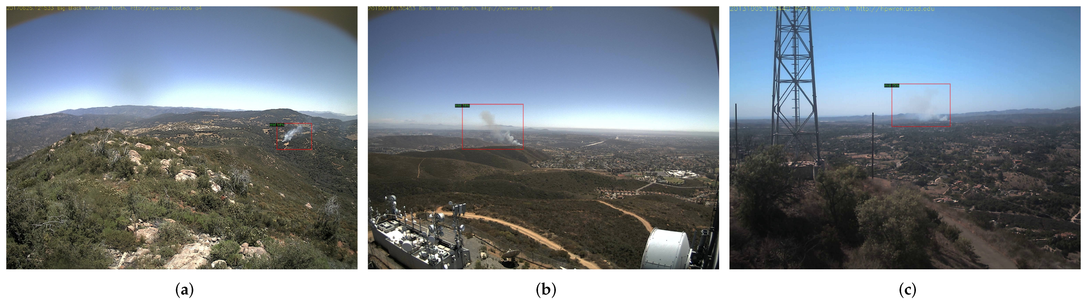
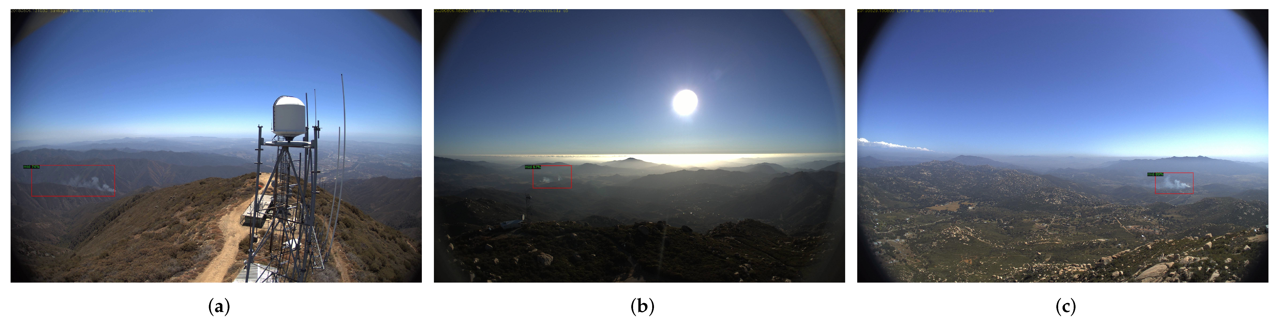
Figure 4 shows three images of sequences that were first detected (with a smoke object) later than 15 min by the model with the best results FRCNN_5000_WUP_3AE. Regarding these negative results, the small dimension of the smoke column (due to the large distance from the lookout) may cause a later first detection as it can be seen Figure 4a, although Figure 5b shows an example of a small fire that was detected early. The saturation of the background of the images may also delay the detection of smoke which is above the horizon as it can be observed in Figure 4b,c. It is noted that examples of early smoke detections have also been represented in Figure 5, which shows three samples with a detection time lower than 5 min.
Moreover, the detection time in forest fires was also calculated for the 75 sequences of images in the test set, as described in Section 3.1. A mean value of 5.3 min for the first detection was obtained with the FRCNN_5000_CYC version with the 3AE configuration and a mean value of 5.4 min with the FRCNN_5000_WUP version with the 3AE configuration. This value is similar to the one obtained using the HPWREN database, even though the average time elapsed between these images is 380 s which is higher than the ones originated from the HPWREN (60 s).
4.5. Limitations
The limitation of this study is that most of the images assembled for the training and testing datasets and also for the HPWREN dataset have a clear view of the horizon without obstructions. The obstructions which are located close to the camera can eventually produce some false smoke detections, so artefact detection or removal techniques need to be designed to increase the feasibility of the system in such situations. A second limitation is that all the datasets are originated from day-time time-series, leading to a problem of solving night-time detection of fires, which is not discussed in this paper. Moreover, the nature of the fire was not controlled in the examples of the employed datasets, so the time elapsed from the fire ignition until the fire is detected can be affected by the magnitude of the initial available natural fuel or the fire propagation speed.
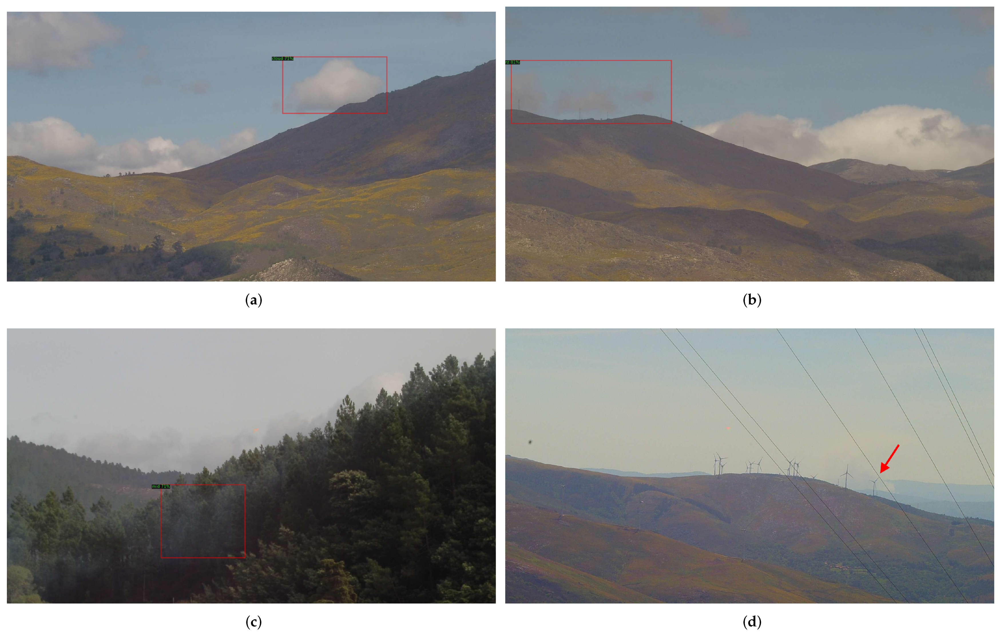
The existence of clouds with similar characteristics to smoke columns may limit the proposed method. Figure 6a shows an example of a correctly identified as a cloud object, while Figure 6b shows an example of an incorrectly identified cloud as an hrz object. The main difference between both objects is the shape and colour, where the first is denser and has whiter shades, while the second is similar to smoke objects, being less dense and with grey shades. Figure 6c shows an example of the morning fog, which can also be interpreted wrongly as a smoke column (in this case it was detected as a mid object. Morning fog objects also have a less dense border and can have similar shapes to smoke columns. Finally, Figure 6d shows an example of a smoke column that was not correctly identified, mainly due to its low visibility, due to background saturation, and the presence of structures (windmill and cables) in front of the smoke column.
5. Conclusions
A deep learning object detection model based on the Detectron2 platform was implemented for smoke detection in outdoor fires. The deep learning model was obtained from transfer-learning of pre-trained RetinaNet and Faster R-CNN models for object detection. The datasets, which were used to re-train the models, and were compounded following different strategies. A DTR of over 86% and an F1-score of over 80% at the fourth image were obtained for an independent test set by the two best models. Both of these models were trained with the dataset labelled with hrz, mid and low smoke classes and with augmentation; Faster R-CNN was the model architecture, they were re-trained during the same iterations but following different learning rate schedules, namely: FRCNN_5000_WUP and FRCNN_5000_CYC.
The proposed models were also tested in a time series dataset which are sequenced with a time resolution of one minute. This database is publicly available and a smoke detection assessment of some examples of this database was previously reported [43]. The time elapsed from the start of the fire until it is first detected was 5.5 min on average for the same 8 sequences of this dataset that were previously reported [43]. Moreover, this time is 6.3 min on average for a total number of 24 sequences of the HPWREN dataset. Using the 75 sequences of the test dataset, a mean detection time of 5.4 min was obtained, maintaining similar performance to the observed with the independent HPWREN dataset. It is important to note that both datasets were acquired using different hardware and in different geographic settings (Portugal and South California), which also shows that our system might be able to adapt to novel conditions. These times can already be considered to have the appropriate specifications to be integrated into a commercial system and can provide an early warning of outdoor fires to the fire prevention authorities.
In the future, it will be important to analyze the temporal evolution of the shape of the smoke column, as it might provide additional help in distinguishing it from other objects such as clouds or smog. After the detection of an object, it will also be beneficial to apply post-processing techniques inside the bounding box. These image processing techniques will be able to segment the detected objects, namely when smoke was found (true positive and all the false detections), inside the bounding boxes and will provide additional information, such as specific features of the objects (namely, spectral, texture and shape) that will be able to be used as an input to recognise some of the mistakes done during the previous object detection steps and increase the recognition rate of this system.
Author Contributions
Conceptualisation, All Authors; methodology, F.G.-F., L.M. and R.V.d.A.; software, F.G.-F., L.M. and R.V.d.A. validation, F.G.-F. and L.M.; formal analysis, F.G.-F. and L.M.; investigation, F.G.-F. and L.M.; resources, H.G. and P.V.; data curation, F.G.-F. and L.M.; writing—original draft preparation, F.G.-F. and L.M.; writing—review and editing, All Authors; visualisation, F.G.-F. and L.M.; supervision, H.G. and P.V.; project administration, H.G. and P.V.; funding acquisition, H.G. and P.V.; All authors have read and agreed to the published version of the manuscript.
Funding
This research has been supported by project POCI-01-0247-FEDER- 038342 from the COMPETE 2020 program.
Institutional Review Board Statement
Not applicable.
Informed Consent Statement
Not applicable.
Data Availability Statement
The data presented in this study is available on request from the corresponding author. The HPWREN data is publicly available from the High Performance Wireless Research and Education Network website.
Acknowledgments
The authors would like to thank Future-Compta S.A for supporting this research work. This project has been supported by project POCI-01-0247-FEDER- 038342 from the COMPETE 2020 program.
Conflicts of Interest
The authors declare no conflict of interest. The funders had no role in the design of the study; in the collection, analyses, or interpretation of data; in the writing of the manuscript, or in the decision to publish the results.
References
- Giglio, L.; Boschetti, L.; Roy, D.P.; Humber, M.L.; Justice, C.O. The Collection 6 MODIS burned area mapping algorithm and product. Remote Sens. Environ. 2018, 217, 72–85. [Google Scholar] [CrossRef]
- Jain, P.; Coogan, S.C.; Subramanian, S.G.; Crowley, M.; Taylor, S.; Flannigan, M.D. A review of machine learning applications in wildfire science and management. Environ. Rev. 2020, 28, 478–505. [Google Scholar] [CrossRef]
- Milne, M.; Clayton, H.; Dovers, S.; Cary, G.J. Evaluating benefits and costs of wildland fires: Critical review and future applications. Environ. Hazards 2014, 13, 114–132. [Google Scholar] [CrossRef]
- Finlay, S.E.; Moffat, A.; Gazzard, R.; Baker, D.; Murray, V. Health Impacts of Wildfires. PLoS Curr. 2012, 4, e4f959951cce2c. [Google Scholar] [CrossRef] [PubMed]
- Haikerwal, A.; Reisen, F.; Sim, M.R.; Abramson, M.J.; Meyer, C.P.; Johnston, F.H.; Dennekamp, M. Impact of smoke from prescribed burning: Is it a public health concern? J. Air Waste Manag. Assoc. 2015, 65, 592–598. [Google Scholar] [CrossRef] [Green Version]
- Oliveira, M.; Delerue-Matos, C.; Pereira, M.C.; Morais, S. Environmental particulate matter levels during 2017 large forest fires and megafires in the center region of Portugal: A public health concern? Int. J. Environ. Res. Public Health 2020, 17, 1032. [Google Scholar] [CrossRef] [Green Version]
- Jaffe, D.A.; Wigder, N.L. Ozone production from wildfires: A critical review. Atmos. Environ. 2012, 51, 1–10. [Google Scholar] [CrossRef]
- Abedi, R. Forest fires (investigation of causes, damages and benefits). New Sci. Technol. 2020, 2, 183–187. [Google Scholar]
- Alkhatib, A.A.A. A Review on Forest Fire Detection Techniques. Int. J. Distrib. Sens. Netw. 2014, 10, 597368. [Google Scholar] [CrossRef] [Green Version]
- Vipin, V. Image Processing Based Forest Fire Detection. Int. J. Emerg. Technol. Adv. Eng. 2012, 2, 87–95. [Google Scholar]
- Barmpoutis, P.; Papaioannou, P.; Dimitropoulos, K.; Grammalidis, N. A review on early forest fire detection systems using optical remote sensing. Sensors 2020, 20, 6442. [Google Scholar] [CrossRef]
- Yu, L.; Wang, N.; Meng, X. Real-time forest fire detection with wireless sensor networks. In Proceedings of the 2005 International Conference on Wireless Communications, Networking and Mobile Computing, WCNM 2005, Wuhan, China, 26 September 2005; Volume 2, pp. 1214–1217. [Google Scholar] [CrossRef]
- Martyn, I.; Petrov, Y.; Stepanov, S.; Sidorenko, A.; Vagizov, M. Monitoring forest fires and their consequences using MODIS spectroradiometer data. IOP Conf. Ser. Earth Environ. Sci. 2020, 507, 12019. [Google Scholar] [CrossRef]
- Manyangadze, T. Forest Fire Detection for Near Real-Time Monitoring Using Geostationary Satellites; International Institute for Geo-Information Science and Earth Observation: Enschede, The Netherlands, 2009. [Google Scholar]
- Ba, R.; Chen, C.; Yuan, J.; Song, W.; Lo, S. SmokeNet: Satellite Smoke Scene Detection Using Convolutional Neural Network with Spatial and Channel-Wise Attention. Remote Sens. 2019, 11, 1702. [Google Scholar] [CrossRef] [Green Version]
- Szegedy, C.; Vanhoucke, V.; Ioffe, S.; Shlens, J.; Wojna, Z. Rethinking the Inception Architecture for Computer Vision. In Proceedings of the 2016 IEEE Conference on Computer Vision and Pattern Recognition (CVPR), Las Vegas, NV, USA, 27–30 June 2016; pp. 2818–2826. [Google Scholar] [CrossRef] [Green Version]
- Priya, R.S.; Vani, K. Deep learning based forest fire classification and detection in satellite images. In Proceedings of the 11th International Conference on Advanced Computing, ICoAC 2019, Chennai, India, 18–20 December 2019; pp. 61–65. [Google Scholar] [CrossRef]
- Hough, G. ForestWatch—A long-range outdoor wildfire detection system. In Proceedings of the WILDFIRE 2007—4th International Wildland Fire Conference, Sevilla, Spain, 13–17 May 2007. [Google Scholar]
- Valente De Almeida, R.; Vieira, P. Forest Fire Finder-DOAS application to long-range forest fire detection. Atmos. Meas. Tech. 2017, 10, 2299–2311. [Google Scholar] [CrossRef] [Green Version]
- Valente de Almeida, R.; Crivellaro, F.; Narciso, M.; Sousa, A.; Vieira, P. Bee2Fire: A Deep Learning Powered Forest Fire Detection System. In Proceedings of the 12th International Conference on Agents and Artificial Intelligence, Valletta, Malta, 22–24 February 2020; SCITEPRESS-Science and Technology Publications: Setúbal, Portugal, 2020; Volume 2, pp. 603–609. [Google Scholar] [CrossRef]
- Li, P.; Zhao, W. Image fire detection algorithms based on convolutional neural networks. Case Stud. Therm. Eng. 2020, 19, 100625. [Google Scholar] [CrossRef]
- Larsen, A.; Hanigan, I.; Reich, B.J.; Qin, Y.; Cope, M.; Morgan, G.; Rappold, A.G. A deep learning approach to identify smoke plumes in satellite imagery in near-real time for health risk communication. J. Expo. Sci. Environ. Epidemiol. 2021, 31, 170–176. [Google Scholar] [CrossRef] [PubMed]
- Toan, N.T.; Thanh Cong, P.; Viet Hung, N.Q.; Jo, J. A deep learning approach for early wildfire detection from hyperspectral satellite images. In Proceedings of the 2019 7th International Conference on Robot Intelligence Technology and Applications (RiTA), Daejeon, Korea, 1–3 November 2019; pp. 38–45. [Google Scholar] [CrossRef]
- Tang, Z.; Liu, X.; Chen, H.; Hupy, J.; Yang, B. Deep Learning Based Wildfire Event Object Detection from 4K Aerial Images Acquired by UAS. AI 2020, 1, 166–179. [Google Scholar] [CrossRef]
- Xiao, Y.; Tian, Z.; Yu, J.; Zhang, Y.; Liu, S.; Du, S.; Lan, X. A review of object detection based on deep learning. Multimed. Tools Appl. 2020, 79, 23729–23791. [Google Scholar] [CrossRef]
- Zou, Z.; Shi, Z.; Guo, Y.; Ye, J. Object Detection in 20 Years: A Survey. arXiv 2019, arXiv:1905.05055. [Google Scholar]
- Wu, X.; Sahoo, D.; Hoi, S.C. Recent advances in deep learning for object detection. Neurocomputing 2020, 396, 39–64. [Google Scholar] [CrossRef] [Green Version]
- Redmon, J.; Divvala, S.; Girshick, R.; Farhadi, A. You Only Look Once: Unified, Real-Time Object Detection. In Proceedings of the 2016 IEEE Conference on Computer Vision and Pattern Recognition (CVPR), Las Vegas, NV, USA, 27–30 June 2016; Volume 2016, pp. 779–788. [Google Scholar] [CrossRef] [Green Version]
- Redmon, J.; Farhadi, A. YOLO9000: Better, faster, stronger. In Proceedings of the IEEE Conference on Computer Vision and Pattern Recognition, Honolulu, HI, USA, 21–26 July 2017; pp. 7263–7271. [Google Scholar]
- Redmon, J.; Farhadi, A. YOLOv3: An Incremental Improvement. arXiv 2018, arXiv:1804.02767. [Google Scholar]
- Bochkovskiy, A.; Wang, C.Y.; Liao, H.Y.M. YOLOv4: Optimal Speed and Accuracy of Object Detection. arXiv 2020, arXiv:2004.10934. [Google Scholar]
- Liu, W.; Anguelov, D.; Erhan, D.; Szegedy, C.; Reed, S.; Fu, C.Y.; Berg, A.C. SSD: Single shot multibox detector. In European Conference on Computer Vision; Lecture Notes in Computer Science (including subseries Lecture Notes in Artificial Intelligence and Lecture Notes in Bioinformatics); Springer: Cham, Switzerland, 2016; pp. 21–37. [Google Scholar] [CrossRef] [Green Version]
- Lin, T.Y.; Goyal, P.; Girshick, R.; He, K.; Dollar, P. Focal Loss for Dense Object Detection. IEEE Trans. Pattern Anal. Mach. Intell. 2020, 42, 318–327. [Google Scholar] [CrossRef] [PubMed] [Green Version]
- Lin, T.Y.; Dollar, P.; Girshick, R.; He, K.; Hariharan, B.; Belongie, S. Feature Pyramid Networks for Object Detection. In Proceedings of the 2017 IEEE Conference on Computer Vision and Pattern Recognition (CVPR), Honolulu, HI, USA, 21–26 July 2017; pp. 936–944. [Google Scholar] [CrossRef] [Green Version]
- Girshick, R.; Donahue, J.; Darrell, T.; Malik, J. Rich feature hierarchies for accurate object detection and semantic segmentation. In Proceedings of the IEEE Computer Society Conference on Computer Vision and Pattern Recognition, Columbus, OH, USA, 24–27 June 2014; pp. 580–587. [Google Scholar] [CrossRef] [Green Version]
- Girshick, R. Fast r-cnn. In Proceedings of the IEEE International Conference on Computer Vision, Santiago, Chile, 7–13 December 2015; pp. 1440–1448. [Google Scholar]
- He, K.; Zhang, X.; Ren, S.; Sun, J. Deep residual learning for image recognition. In Proceedings of the IEEE Computer Society Conference on Computer Vision and Pattern Recognition, Las Vegas, NV, USA, 27–30 June 2016; Volume 2016, pp. 770–778. [Google Scholar] [CrossRef] [Green Version]
- Simonyan, K.; Zisserman, A. Very deep convolutional networks for large-scale image recognition. In Proceedings of the 3rd International Conference on Learning Representations, ICLR 2015-Conference Track Proceedings, San Diego, CA, USA, 7–9 May 2015. [Google Scholar]
- Barmpoutis, P.; Dimitropoulos, K.; Kaza, K.; Grammalidis, N. Fire Detection from Images Using Faster R-CNN and Multidimensional Texture Analysis. In Proceedings of the ICASSP 2019-2019 IEEE International Conference on Acoustics, Speech and Signal Processing (ICASSP), Brighton, UK, 12–17 May 2019; pp. 8301–8305. [Google Scholar] [CrossRef]
- Zhang, Q.X.; Lin, G.H.; Zhang, Y.M.; Xu, G.; Wang, J.J. Wildland Forest Fire Smoke Detection Based on Faster R-CNN using Synthetic Smoke Images. Procedia Eng. 2018, 211, 441–446. [Google Scholar] [CrossRef]
- Xu, R.; Lin, H.; Lu, K.; Cao, L.; Liu, Y. A Forest Fire Detection System Based on Ensemble Learning. Forests 2021, 12, 217. [Google Scholar] [CrossRef]
- Valikhujaev, Y.; Abdusalomov, A.; Cho, Y.I. Automatic Fire and Smoke Detection Method for Surveillance Systems Based on Dilated CNNs. Atmosphere 2020, 11, 1241. [Google Scholar] [CrossRef]
- Pan, H.; Badawi, D.; Cetin, A.E. Computationally efficient wildfire detection method using a deep convolutional network pruned via fourier analysis. Sensors 2020, 20, 2891. [Google Scholar] [CrossRef]
- Park, M.; Tran, D.Q.; Jung, D.; Park, S. Wildfire-Detection Method Using DenseNet and CycleGAN Data Augmentation-Based Remote Camera Imagery. Remote Sens. 2020, 12, 3715. [Google Scholar] [CrossRef]
- Witten, I.H.; Frank, E.; Hall, M.A. Data Mining: Practical Machine Learning Tools and Techniques, 3rd ed.; Morgan Kaufmann Publishers Inc.: San Francisco, CA, USA, 2011; pp. 1–622. [Google Scholar]
- University of California San Diego, California, America: The High Performance Wireless Research and Education Network, HPWREN Dataset. 2021. Available online: http://hpwren.ucsd.edu/index.html (accessed on 30 August 2021).
- Wong, K.H. OpenLabeler. 2020. Available online: https://github.com/kinhong/OpenLabeler (accessed on 10 May 2021).
- Lin, T.Y.; Maire, M.; Belongie, S.; Hays, J.; Perona, P.; Ramanan, D.; Dollár, P.; Zitnick, C.L. Microsoft COCO: Common Objects in Context BT. In Computer Vision—ECCV 2014; Fleet, D., Pajdla, T., Schiele, B., Tuytelaars, T., Eds.; Springer International Publishing: Cham, Switzerland, 2014; pp. 740–755. [Google Scholar]
- Gao, L.; He, Y.; Sun, X.; Jia, X.; Zhang, B. Incorporating negative sample training for ship detection based on deep learning. Sensors 2019, 19, 684. [Google Scholar] [CrossRef] [PubMed] [Green Version]
- Buslaev, A.; Iglovikov, V.I.; Khvedchenya, E.; Parinov, A.; Druzhinin, M.; Kalinin, A.A. Albumentations: Fast and flexible image augmentations. Information 2020, 11, 125. [Google Scholar] [CrossRef] [Green Version]
- Wu, Y.; Kirillov, A.; Massa, F.; Lo, W.Y.; Girshick, R. Detectron2. 2019. Available online: https://0-doi-org.brum.beds.ac.uk/https://github.com/facebookresearch/detectron2 (accessed on 1 September 2021).
- Smith, L.N. Cyclical learning rates for training neural networks. In Proceedings of the 2017 IEEE Winter Conference on Applications of Computer Vision, WACV 2017, Santa Rosa, CA, USA, 24–31 March 2017; pp. 464–472. [Google Scholar] [CrossRef] [Green Version]
Figure 1.
Different types of identified fire smoke columns. (a) Example of smoke labelled as hrz. Taken at 21 July 2014 15:24 (b) Example of smoke labelled as mid. Taken at 15 May 2015 13:01 (c) Example of smoke labelled as low. Taken at 20 July 2013 12:29.
Figure 1.
Different types of identified fire smoke columns. (a) Example of smoke labelled as hrz. Taken at 21 July 2014 15:24 (b) Example of smoke labelled as mid. Taken at 15 May 2015 13:01 (c) Example of smoke labelled as low. Taken at 20 July 2013 12:29.

Figure 2.
This is an example of a temporal sequence of smoke fire from before the fire stars until 5 images after the beginning of the fire. (a) Example of just before fire starts. Examples (b–f) are consecutive images after the fire starts. The red boxes show the area detected as smoke by our method FRCNN_5000_CYC trained with dataset 3AE. The image sequence was taken on the same day, 10 March 2014, respectively at 9:23, 9:29, 9:36, 9:42, 9:49 and 9:56.

Figure 3.
Illustrative examples of the 20180504_FIRE_smer-tcs8-mobo-c video sequence, (a) showing the zero reference from database; (b) showing the fire ignition (see red arrow) with a time reference of 11 min later defined by us and (c) showing the next image, one minute later. The image sequence was taken in the same day, 4 May 2018, respectively at 14:33, 14:44 and 14:45.

Figure 4.
(a) 20170625_BBM_bm-n-mobo was taken at 25 June 2017 12:15 (b) 20190716_FIRE_bl-s-mobo-c was taken at 16 July 2019 13:04 and (c) DeLuz Fire was taken at 05 October 2013 12:54. The red boxes show the area detected as smoke by our method FRCNN_5000_WUP trained with dataset 3AE.
Figure 4.
(a) 20170625_BBM_bm-n-mobo was taken at 25 June 2017 12:15 (b) 20190716_FIRE_bl-s-mobo-c was taken at 16 July 2019 13:04 and (c) DeLuz Fire was taken at 05 October 2013 12:54. The red boxes show the area detected as smoke by our method FRCNN_5000_WUP trained with dataset 3AE.

Figure 5.
(a) Holy Fire South View was taken at 6 August 2018 13:10 (b) 20200806_SpringsFire_lp-w-mobo-c was taken at 6 August 2020 18:36 and (c) 20190529_94Fire_lp-s-mobo was taken at 29 May 2019 15:08. The red boxes show the area detected as smoke by our method FRCNN_5000_WUP trained with dataset 3AE.

Figure 6.
(a) Example of a correctly identified cloud object. Taken at 22 June 2015 17:30. (b) Example of a cloud incorrectly identified as a smoke object. Taken at 22 June 2015 17:38. (c) Example of fog, incorrectly identified as a smoke object. Taken at 25 April 2015 10:13, (d) Example of a smoke object that was not correctly identified. Taken at 21 May 2015 15:22.


Table 1.
Characteristics of the dataset for training and validation. Y means yes, images with this characteristic were included in the dataset and N means no, the images with this characteristic were not included. A means augmentation, C means clouds and E images without any annotation.
Table 1.
Characteristics of the dataset for training and validation. Y means yes, images with this characteristic were included in the dataset and N means no, the images with this characteristic were not included. A means augmentation, C means clouds and E images without any annotation.
| Version | Characteristics | Number of Images with Object | ||||||||
|---|---|---|---|---|---|---|---|---|---|---|
| # Smoke Classes | Aug | Clouds | Empty | Smoke | Clouds | Empty | Hrz | Mid | Low | |
| 1 | 1 | N | N | N | 750 | 0 | 0 | 0 | 0 | 0 |
| 1A | 1 | Y | N | N | 1500 | 0 | 0 | 0 | 0 | 0 |
| 1C | 1 | N | Y | N | 750 | 750 | 0 | 0 | 0 | 0 |
| 1AC | 1 | Y | Y | N | 1500 | 1500 | 0 | 0 | 0 | 0 |
| 3 | 3 | N | N | N | 0 | 0 | 0 | 111 | 490 | 200 |
| 3A | 3 | Y | N | N | 0 | 0 | 0 | 222 | 980 | 400 |
| 3C | 3 | N | Y | N | 0 | 750 | 0 | 111 | 490 | 200 |
| 3AC | 3 | Y | Y | N | 0 | 1500 | 0 | 222 | 980 | 400 |
| 1E | 1 | N | N | Y | 750 | 0 | 750 | 0 | 0 | 0 |
| 1AE | 1 | Y | N | Y | 1500 | 0 | 1500 | 0 | 0 | 0 |
| 1CE | 1 | N | Y | Y | 750 | 750 | 750 | 0 | 0 | 0 |
| 1ACE | 1 | Y | Y | Y | 1500 | 1500 | 1500 | 0 | 0 | 0 |
| 3E | 3 | N | N | Y | 0 | 0 | 750 | 111 | 490 | 200 |
| 3AE | 3 | Y | N | Y | 0 | 0 | 1500 | 222 | 980 | 400 |
| 3CE | 3 | N | Y | Y | 0 | 750 | 750 | 111 | 490 | 200 |
| 3ACE | 3 | Y | Y | Y | 0 | 1500 | 1500 | 222 | 980 | 400 |
Table 2.
Classification performance metrics in the test set. F1i means the F1-score of the image at the position ith of the fire sequence and the FPRC and FPRE denote the false-positive ratio for cloud and empty images respectively.
Table 2.
Classification performance metrics in the test set. F1i means the F1-score of the image at the position ith of the fire sequence and the FPRC and FPRE denote the false-positive ratio for cloud and empty images respectively.
| Version | F11 (%) | F12 (%) | F13 (%) | F14 (%) | F15 (%) | FPRC (%) | FPRE (%) | FPRT (%) | G-Mean (%) |
|---|---|---|---|---|---|---|---|---|---|
| RetinaNet 3500_WUP | |||||||||
| 3AC | 58.6 | 60.8 | 67.3 | 70.8 | 68.5 | 4.6 | 3.3 | 4.5 | 70.5 |
| 1 | 54.2 | 69.7 | 68.4 | 71.9 | 68.5 | 18.7 | 5.6 | 11.4 | 66.9 |
| 1CE | 29.3 | 31.0 | 29.5 | 30.2 | 24.7 | 0.1 | 0.0 | 0.3 | 41.7 |
| RetinaNet 5000_WUP | |||||||||
| 1A | 55.1 | 69.7 | 68.4 | 69.6 | 74.3 | 12.1 | 2.4 | 6.9 | 71.7 |
| 1 | 60.0 | 69.7 | 67.3 | 71.9 | 70.9 | 18.3 | 5.2 | 11.0 | 70.4 |
| 3CE | 35.3 | 47.3 | 45.4 | 54.0 | 50.5 | 0.4 | 0.0 | 0.4 | 55.9 |
| FRCNN 5000_WUP | |||||||||
| 3AE | 64.1 | 75.4 | 68.4 | 84.1 | 78.6 | 6.3 | 1.9 | 4.4 | 78.6 |
| 3CE | 61.4 | 69.7 | 69.6 | 76.3 | 74.3 | 3.1 | 0.7 | 2.6 | 76.3 |
| 3E | 52.6 | 53.6 | 51.5 | 61.0 | 55.1 | 0.8 | 0.2 | 1.2 | 63.4 |
| FRCNN 5000_CYC | |||||||||
| 3AE | 69.2 | 75.4 | 78.0 | 80.3 | 75.4 | 6.7 | 2.7 | 5.2 | 80.1 |
| 3E | 64.1 | 74.3 | 69.6 | 71.9 | 67.9 | 4.8 | 1.4 | 3.7 | 75.3 |
| 1E | 22.8 | 36.8 | 33.3 | 37.8 | 38.6 | 1.2 | 0.2 | 2.0 | 48.2 |
Table 3.
Accumulated detection rate for different models over time. The DRTn means the detection rate at the nth image in the smoke sequences.
Table 3.
Accumulated detection rate for different models over time. The DRTn means the detection rate at the nth image in the smoke sequences.
| Version | DTR1 (%) | DTR2 (%) | DTR3 (%) | DTR4 (%) | DTR5 (%) |
|---|---|---|---|---|---|
| RetinaNet_3500_WUP | |||||
| 3AC | 38.7 | 57.3 | 68.0 | 77.3 | 85.3 |
| 1 | 34.7 | 60.0 | 72.0 | 78.7 | 85.3 |
| 1CE | 16.0 | 26.7 | 29.3 | 33.3 | 37.3 |
| RetinaNet_5000_WUP | |||||
| 1A | 34.7 | 54.7 | 66.7 | 76.0 | 80.0 |
| 1 | 40.0 | 62.7 | 69.3 | 77.3 | 82.7 |
| 3CE | 20.0 | 37.3 | 46.7 | 56.0 | 61.3 |
| FRCNN_5000_WUP | |||||
| 3AE | 42.7 | 68.0 | 73.3 | 86.7 | 89.3 |
| 3CE | 41.3 | 61.3 | 68.0 | 77.3 | 85.3 |
| 3E | 33.3 | 46.7 | 49.3 | 60.0 | 62.7 |
| FRCNN_5000_CYC | |||||
| 3AE | 48.0 | 69.3 | 80.0 | 86.7 | 92.0 |
| 3E | 44.0 | 66.7 | 72.0 | 80.0 | 82.7 |
| 1E | 12.0 | 28.0 | 34.7 | 40.0 | 44.0 |
Table 4.
Average precision for the selected models in the validation dataset.
| Version | AP (%) | AP50 (%) | AP75 (%) |
|---|---|---|---|
| RetinaNet_3500_WUP | |||
| 3AC | 38.7 | 75.0 | 36.7 |
| 1 | 39.6 | 83.3 | 31.3 |
| 1CE | 38.0 | 71.3 | 35.7 |
| RetinaNet_5000_WUP | |||
| 1A | 52.2 | 87.7 | 53.6 |
| 1 | 42.0 | 84.5 | 37.5 |
| 3CE | 38.9 | 72.3 | 39.4 |
| FRCNN_5000_WUP | |||
| 3AE | 40.1 | 81.2 | 31.6 |
| 3CE | 34.1 | 67.1 | 30.9 |
| 3E | 37.8 | 74.4 | 33.9 |
| FRCNN_5000_CYC | |||
| 3AE | 36.0 | 73.8 | 32.2 |
| 3E | 38.7 | 73.9 | 36.5 |
| 1E | 24.3 | 55.3 | 16.4 |
Table 5.
Daytime Fire Detection Time of smoke sequences extracted from HPWREN Database. The best results for each case study are marked in bold.
Table 5.
Daytime Fire Detection Time of smoke sequences extracted from HPWREN Database. The best results for each case study are marked in bold.
| Video Name | Time Elapsed (min) | |||
|---|---|---|---|---|
| Method [43] | FRCNN 5000 CYC 3AE | FRCNN 5000 WUP 3AE | RetinaNet 3500 WUP 1CE | |
| Lyons Fire | 8 | 5 | 5 | 8 |
| Holy Fire East View | 11 | 3 | 2 | 4 |
| Holy Fire South View | 9 | 2 | 1 | 2 |
| Palisades Fire | 3 | 7 | 5 | 9 |
| Palomar Mountain Fire | 13 | 18 | 10 | 16 |
| Highway Fire | 2 | 4 | 2 | 9 |
| Tomahawk Fire | 5 | 5 | 3 | 5 |
| DeLuz Fire | 11 | 22 | 16 | 136 |
| 20190529_94Fire_lp-s-mobo-c | N.A | 3 | 3 | 3 |
| 20190610_FIRE_bh-w-mobo-c | N.A | 6 | 5 | N.D |
| 20190716_FIRE_bl-s-mobo-c | N.A | 18 | 18 | N.D |
| 20190924_FIRE_sm-n-mobo-c | N.A | 17 | 7 | N.D |
| 20200611_skyline_lp-n-mobo-c | N.A | 5 | 4 | N.D |
| 20200806_SpringsFire_lp-w-mobo-c | N.A | 8 | 1 | 37 |
| 20200822_BrattonFire_lp-e-mobo-c | N.A | 2 | 5 | N.D |
| 20200905_ValleyFire_lp-n-mobo-c | N.A | 4 | 3 | N.D |
| 20160722_FIRE_mw-e-mobo-c | N.A | 3 | 5 | N.D |
| 20170520_FIRE_lp-s-iqeye | N.A | 8 | 2 | N.D |
| 20170625_BBM_bm-n-mobo | N.A | 23 | 21 | 25 |
| 20170708_Whittier_syp-n-mobo-c | N.A | 4 | 5 | 6 |
| 20170722_FIRE_so-s-mobo-c | N.A | 6 | 13 | 27 |
| 20180504_FIRE_smer-tcs8-mobo-c | N.A | 7 | 9 | 16 |
| 20180504_FIRE_smer-tcs8-mobo-c | N.A | 4 | 3 | 9 |
| 20180809_FIRE_mg-w-mobo-c | N.A | 6 | 2 | N.D |
| Mean ± sd for 1–8 | 7.8 ± 3.8 | 8.3 ± 7.7 | 5.5 ± 8.7 | 23.6 ± 9.7 |
| Mean ± sd for 1–24 | 7.9 ± 6.3 | 6.3 ± 5.4 | 20.8 ± 32.3 | |
1 Not available; 2 Not detected.
Publisher’s Note: MDPI stays neutral with regard to jurisdictional claims in published maps and institutional affiliations. |
© 2021 by the authors. Licensee MDPI, Basel, Switzerland. This article is an open access article distributed under the terms and conditions of the Creative Commons Attribution (CC BY) license (https://creativecommons.org/licenses/by/4.0/).
Share and Cite
MDPI and ACS Style
Guede-Fernández, F.; Martins, L.; de Almeida, R.V.; Gamboa, H.; Vieira, P. A Deep Learning Based Object Identification System for Forest Fire Detection. Fire 2021, 4, 75. https://0-doi-org.brum.beds.ac.uk/10.3390/fire4040075
AMA Style
Guede-Fernández F, Martins L, de Almeida RV, Gamboa H, Vieira P. A Deep Learning Based Object Identification System for Forest Fire Detection. Fire. 2021; 4(4):75. https://0-doi-org.brum.beds.ac.uk/10.3390/fire4040075
Chicago/Turabian StyleGuede-Fernández, Federico, Leonardo Martins, Rui Valente de Almeida, Hugo Gamboa, and Pedro Vieira. 2021. "A Deep Learning Based Object Identification System for Forest Fire Detection" Fire 4, no. 4: 75. https://0-doi-org.brum.beds.ac.uk/10.3390/fire4040075