
Long Term Post-Fire Vegetation Dynamics in North-East Mediterranean Ecosystems. The Case of Mount Athos Greece


1
Department of Forestry and Natural Environment, International Hellenic University, 1st km Drama-Mikrohori, GR66100 Drama, Greece
2
Peter Buckley Associates, Oast Barn, 37a The Green, Woodchurch, Ashford TN26 3PF, UK
3
School of Biological Sciences, University of Reading, Whiteknights, Reading RG6 6AS, UK
*
Author to whom correspondence should be addressed.
Fire 2021, 4(4), 92; https://0-doi-org.brum.beds.ac.uk/10.3390/fire4040092
Submission received: 7 October 2021
/
Revised: 3 December 2021
/
Accepted: 4 December 2021
/
Published: 8 December 2021
(This article belongs to the Special Issue Multi-Source and Multi-System Fire Monitoring Relying on EO Data in Mediterranean Ecosystems)
Abstract
:Fire is an ecological and disturbance factor with a significant historical role in shaping the landscape of fire-prone environments. Despite the large amount of literature regarding post-fire vegetation dynamics, the north-east Mediterranean region is rather underrepresented in the literature. Studies that refer to the early post fire years and long term research are rather scarce. The current study is conducted in the socially and geographically isolated peninsula of Mount Athos (Holly Mountain) in northern Greece, and it studies vegetation dynamics over a period of 30 years since the last fire. Field data were collected 11 years since the event and were used to identify the present plant communities in the area, using TWINSPAN, and the factors affecting their distribution using CART. Four Landsat (TM, ETM, OLI) images are employed for the calculation of NDVI, which was found effective in detecting the intercommunity variation in the study area, and it is used for long term monitoring. The study includes four communities, from maquis to forest which are common in the Mediterranean region covering a wide altitudinal range. The results suggest that fire affects the various communities in a different way and their recovery differs significantly. While forest communities recover quickly after fire, maintaining their composition and structure, the maquis communities may need several years before reaching the pre-fire characteristics. The dry climatic conditions of the study area are probably the reason for the slow recovery of the most fire prone communities. Given that climate change is expected to make the conditions even drier in the region, studies like this emphasize the need to adopt measures for controlling wildfires and preventing ecosystem degradation.
1. Introduction
Fire is an important ecological factor that affects both the structure and distribution of many plant communities throughout the world. Fire probably first appeared, as a natural disturbance factor as soon as there was any existing terrestrial vegetation [1,2,3]. Prior to human influence the main ignition sources were lightning, volcanic and earthquake activity [4,5,6]. Fire was a periodical ecological process in the vegetation cycle of succession, causing the continued rejuvenation and promoting the productivity of many plant communities and ecosystems [3]. Later, fire became an important human tool, widely used for the improvement of living conditions. The fire characteristic most altered due to human presence is fire frequency, mainly due to the increase of ignition sources. It is worth noting that in the Mediterranean region 98% of the occurring fires are of an anthropogenic origin [7]. The increased frequency and extent of wildfires constitute a major global issue due to their high contribution on atmospheric pollution [8], and their subsequent effect on ecosystem properties and human health [9]. Projection of wildfire activity across the globe under the foreseen global changes in climate patterns, anthropogenic activities and land uses indicate a significant increase in fire frequency by 2050 affecting many regions of the world [10].
In the Mediterranean region, fire has had a significant role in shaping the landscape and determining ecosystems and species distribution and is considered one of the most fire-prone regions in the world [11,12,13,14,15]. After the establishment of the characteristic Mediterranean climate in the region, approximately 2.8 million years ago [16], fire has become one of the major selection forces for the Mediterranean flora, and it is the adaptation of many species to recurrent fires which ensures their persistence [12]. The two main reasons for the frequency of fire in Mediterranean ecosystems are the summer drought and the long human presence in the area [12].
The responses of vegetation to fire and the post-fire succession have been widely studied and there is large literature describing species survival strategies and the post-fire succession. The common denominator in most of these studies is that the post-fire succession does not follow a typical secondary succession pattern in which different species or functional groups succeed one another towards a climax community. Instead, an auto-succession model is followed in which the species that occurred prior to the fire reoccupy their space and regain their pre-fire role in the community quite soon after the event [3,17,18,19,20,21]. The most important survival strategies are vegetative regeneration and resprouting from surviving buds [22,23], or through the establishment of seedlings from seeds stored in the soil [24,25] or on the plant [26]. Resprouting, perhaps the most common survival strategy in most fire-prone environments, appears to be an ancestral trait allowing survival of plants after removal of above ground parts by fire or grazing and cutting [27]. The establishment of seedlings after germination of stored seeds in response to a fire related cue, i.e., high temperature, smoke or burned wood, appears to be a survival strategy selected under the pressure of fire allowing survival of plants after a fire event [24,25]. Both survival strategies are important and they both play a role in the re-establishment of the dynamic equilibrium.
Mediterranean ecosystems and especially maquis communities dominated primarily by Quercus coccifera L. have been studied in relation to their response to fire and the majority of these studies have been carried out in the western part of the Mediterranean region and, more specifically, in France [3,19,20,28,29,30,31], Spain [32,33,34,35] and Portugal [36]. In the eastern part of Mediterranean region most of the fire ecology literature refers to phryganic ecosystems or dwarf shrub ecosystems in Greece [37,38,39,40] or in Israel [41,42]. Similar studies on Mediterranean conifers also exist for the eastern Mediterranean region [18,43,44,45,46,47,48]. Despite the number of studies conducted on the post fire vegetation succession, the north-east Mediterranean region remains rather underrepresented in the literature.
The auto-succession theory states that the time required for the vegetation to regain its pre-fire floristic composition is short, because all species respond promptly to the destructive role of fire. Apart from some changes in species richness which occur during the first 3–4 post-fire years, the pre-fire community re-establishes within a period which, for Q. coccifera dominated communities, can be as low as 3.5 years [32]. It is unlikely, however, that this rapid recovery is the case in all communities in fire-prone environments, even in areas which belong to the same climatic zone. For instance, the eastern Mediterranean region is more arid than the western one, and, although similar plant communities are present in both areas, it would be expected that differences, not in the fundamental principles of the auto-succession but in the relative species abundances in the post-fire environment, would be found. The current study examines the similarities and differences between the established theory of post-fire vegetation succession with results from a more arid environment than in the western Mediterranean region.
The study is conducted in the peninsula of Mount Athos in northern Greece and the aim is to examine the effects of fire in multiple communities ranging from maquis of the lowest altitudes to deciduous forests at higher altitudes over a period of 30 years since the last fire. The objectives of the study are (a) to identify all plant communities present in the study area, (b) to identify the role of fire in shaping their distribution and (c) to determine the period required for a community to recover from fire
2. Materials and Methods
2.1. Study Area
The study is conducted in the geographically and socially isolated peninsula of Mount Athos in northern Greece (40°11′40.01′′ N, 24°13′55.95′′ E; Figure 1), where a monastic life was established more than a thousand years ago and it is now inhabited only by monks and hermits who live either in the 20 monasteries or in isolated cells and hermitages. According to Rackham [49], the social conditions have remained the same for over 1000 years and the absence of domestic animals allowed to avoid the browsing and cultivation activities which have ravaged the rest of the Mediterranean region.
The area has a long history of wildfires which, according to the existing records, occur at relatively large intervals of more than 40 years. In the wider region fires occur during the fire season which coincides with the summer draught period lasting between April and October and most commonly between June and August. The last two known wildfires were in 1945 and in August of 1990 and no fire has occurred in the area since 1990. The current study focuses on these wildfires, and it monitors the vegetation changes and succession over a period of 30 years since the last one. The total size of the study area is 2014 ha. The fire of 1945, according to a visual interpretation of aerial photographs obtained by the Hellenik Military Geographical Service, burned 773 ha of the study area while this of 1990 burned 1,305 ha, including the entire area of 1945. Approximately 710 ha of the site escaped both fires and there are no written or oral records of a fire from the last century until today. As a result, sites located at the unburned part are considered as mature sites and provide the controls for the investigation of the effects of fire on vegetation. Figure 1 shows the parts of the study area under the different fire regimes.
The general orientation of the site is southwest, however, due to the complex and sharp relief, one can find all different aspects from north to south and east to west. The altitudinal range is from the sea level to 889 m; however, the study is confined to up to approximately 500 m which is the part of the area affected by the wildfire of 1990. The climate is Mediterranean with pronounced biseasonality in annual precipitation and a summer drought period. According to the existing data the climate in the areas below 500 m has an annual precipitation of less than 500 mm, mean annual temperature of 15.7 °C, mean annual atmospheric moisture of 70% and 2800 hrs of sunshine per year. Based on those data as well as on the vegetation characteristics of the study area the climate was classified as Csa type according to Koppen which is characterised by hot and dry summers and mild winters [50].
2.2. In Situ Sampling and Data Collection
Field sampling was performed between April and October 2001 for the collection of vegetation and environmental parameters data that will aid the process of understanding the patterns of vegetation distribution. The study area was divided into three zones based on the fire regime with the first zone including the area burned both in 1945 and 1990, the second the area burned only in 1990 and the third the area which has not been burned for more than 60 years. The target was to sample approximately 150 points in total and this number was divided accordingly to the extent of three zones. The 150 points ensure a minimum average sample density of one sample per 25 hectares which according to Tzanopoulos et al. [51] is sufficient to capture the heterogeneity of the Mediterranean landscape. Within each zone, the corresponding number of points was randomly located. The random location of sampled points and the large variation in topographic conditions ensures that the variation in environmental factors and vegetation structure and composition will be sufficiently represented in the dataset.
During sampling, the exact location of the sampled quadrat was adjusted by a few meters if necessary in order to ensure homogeneity in environmental conditions and vegetation characteristics. Their size varied between 300 and 500 m2 depending on vegetation type [52] with smaller-sized quadrats being used to sample maquis vegetation and larger sized for forest vegetation. The four corners and the centre of each quadrat were marked using a GARMIN eTrex Vista GPS with a spatial accuracy of 4 m. In each quadrat the cover of all woody species was visually estimated using a 20-point cover scale. The 20-point cover scale was based on the 9-point Braun-Blanquet cover-abundance scale [53], which was further divided in order to achieve a much more accurate recording of the vegetation composition. For the purposes of data analysis, a smoothing operation was applied where the 20-class scale was converted into percentage cover values using a power regression formula [54]:
Cover (%) = 0.1165 × (Class midpoint)2.2457 (p < 0.0001, R2 = 0.99)
Fifty woody species in total were recorded during the survey. The identification of species was done using [55,56] and the nomenclature follows Flora Europaea (1964–1993).
In addition to species cover, the height of the vegetation was measured as well as the presence of mature individuals on burned sites which had escaped fire. In each quadrat a number of topographical factors were recorded including aspect, slope and altitude using a compass, a clinometer and an altimeter, respectively. From each quadrat five soil samples were taken in a W shape to the depth of 10 cm into the inorganic soil layers. The five samples were air dried for 48 h and then mixed in equal quantities to produce one bulk sample representative for the whole quadrat.
The following physical and chemical soil properties were determined with the aim of investigating their effect on vegetation distribution and composition: Total Organic Nitrogen (N), Total Phosphorus (P), Total Potassium (K), Available Phosphorus (Phosphate), Available Calcium (Ca), Available Magnesium (Mg) Available Potassium, Available Sodium (Na), Organic matter content (OM), pH and soil particle size distribution. Total N, P and K were determined from the same extract produced using the Kjeldahl procedure [57]. For available phosphorus the molybdenum blue method [57,58] was employed after extracting the phosphorus from soil using an 0.5 M sodium bicarbonate reagent (pH = 8.5). Available potassium and magnesium were estimated from the same soil extract using ammonium nitrate as the extraction agent [58]. Available Ca and Na were extracted from the soil using ammonium acetate as the extraction agent [58]. A pH meter [58] was used for pH estimation. The loss-on-ignition method [59] was employed for organic matter content after drying both the porcelain crucibles for 12 h at 105 °C and the soil for another 12 h at 105 °C and then placing the samples in a furnace at 550 °C for 15 h. Soil particle size distribution was determined by using a Buyoucos hydrometer in a water-soil suspension.
2.3. Plant Community Identification
A number of different plant communities are present in the study area. The aim of this analysis is to identify these communities and to explore their main floristic properties as a necessary first step. A sound understanding of the plant community composition is essential to provide a baseline for comparing sites with similar pre-fire vegetation for the study of the plant community patterns in relation to fire. The analysis of vegetation data for the identification of the plant communities and the investigation of some of their main floristic characteristics is carried out in two steps. The plant communities are identified using classification analysis and second an indirect ordination analysis is applied to provide a better insight into their floristic composition as well as information on the floristic relationships between the communities.
The hierarchical polythetic divisive method Two Way INdicator SPecies ANalysis (TWINSPAN) [60,61] was employed in the current study. TWINSPAN is preferred over other hierarchical methods because it uses the whole range of information included in a data matrix and not just the presence or absence of a single species, while it is more robust and less prone to misclassification errors [62]. Compared to traditional table rearrangement methods it is considered much more objective [63]. A disadvantage of TWINSPAN is that it is based on an ordination of samples and species on a single axis and that’s why it is recommended to be followed by an ordination using Detrended Correspondence Analysis (DCA) [62].
TWINSPAN employs the concept of pseudospecies which is a technique for converting quantitative data into qualitative [61]. According to this concept, any species is represented in the classification process by a series of pseudospecies the number of which depends on the species abundance in a particular sample and the applied cut levels which are abundance thresholds. In the current study the six cut levels used by Rodwell [64] for the Natural Vegetation Classification (NVC) of Great Britain were used for the derivation of pseudospecies. These are: 0.1, 4.1, 10.1, 25.1, 33.1 and 50.1. The range of abundances represented by each of the six pseudospecies (in brackets) are: 0.1–4% (1), 4.1–10% (2), 10.1–25% (3), 25.1–33% (4), 33.1–50% (5), >50.1% (6). For the identification of plant communities and their lower divisions the scheme employed by Rodwell [64] was applied where the “community” is the basic unit (without higher hierarchical levels) and it can be divided at lower hierarchical levels into “sub-communities” and “variants”.
For the denomination of communities and sub-communities up to three of the most frequent and abundant species were used. Hence, for every identified group a table of species frequencies and a table of preferential pseudospecies were produced. The latter represents the abundance of the most characteristic species within each group. The term frequency describes how often a species is found among the samples comprising a group regardless of how much of the species is present in a sample. Five frequency classes were identified and each of them is denoted by a Roman numeral: I= 1–20% frequency; II = 21–40%; III = 41–60%; IV = 61–80% and V= more than 80%. Species with frequency classes of IV and V in a particular group are referred as constants; those with frequency class III as common or frequent; those with frequency class II as occasional and those with frequency class I as scarce. On the other hand, the term abundance describes how much of a species is present in a sample. Six abundance levels were identified which are the same as the pseudospecies levels.
The classification process was assisted by a DCA [65] which resulted in two dimensional diagrams along the two axes which summarises the variation in the data. In these diagrams the samples are represented by points which are arranged in such a manner that samples with similar species composition are close to each other and those which are far apart have dissimilar species composition [66]. The ordination analysis was done using the CANOCO for Windows software [67,68].
2.4. Identification of the Factors Determining Community Distribution-Hypothesis Generation
Fire is one of several factors that are expected to have a significant role in shaping community distribution in the study area. The preliminary hypothesis is that fire affects the distribution of communities not in the same way and probably some of them are affected more than others. In order to test this hypothesis and perhaps generate additional ones, classification trees were employed to identify the most important factors determining the distribution of the plant communities. The classification tree approach [69,70] is a powerful method which can deal effectively with the complexity often inherent in ecological data [71]. Classification trees repeatedly divide the data into two mutually exclusive groups on the basis of a single explanatory variable until a set of homogenous groups, in terms of the response variables, is achieved [71], or until the data cannot be divided any further based on the explanatory variables available. At each division the variable that best divides the data is used. Hence, instead of estimating the mean value of a range of environmental factors associated with the communities, classification trees identify specific thresholds of environmental variables above or below which a vegetation type can be found [72].
The classification of each sample into one of the plant communities and sub-communities was used as the response variable. The explanatory variables comprised all of the environmental variables recorded during the fieldwork and in the laboratory such as slope, aspect, altitude, fire regime and soil physical and chemical properties. Among more than 30 different classification trees the most suitable was selected based on two criteria. First, the selected tree should have the lowest misclassification rate and highest kappa statistic which should exceed 0.4 [73,74]. An “honest” misclassification rate was achieved by using 10-fold cross validation [71]. Accordingly, the dataset of 134 samples was split into 10 approximately equal partitions, each of which in turn was used for testing while the remainder was used for training the classifier. The validation procedure was repeated ten times and consequently each sample was used nine times for training the classifier and once for testing it [69]. The second criterion was based on the comparison between the misclassification rate of the tree and the misclassification rate of a tree, built based on the “go with the majority” rule [71]. The “go with the majority” tree (termed the “null model” in the current study) classifies all the data in the group with the highest number of instances and because in this study 54 out of 134 samples belong to the sub-community MQ1a, the misclassification rate of the null model is 60% and the correct classification rate is 40%. Hence, the selected classification tree should have a correct classification rate higher than 40%.
2.5. Remote Sensing Data
Four Landsat images were obtained both for testing the hypotheses built in the analysis of the environmental factors that affect the community distribution as well as for monitoring the vegetation changes in the following 20 years. The first image was a Landsat 4-TM, sensed on the 23 June 1989, one year before the 1990 fire event. The second and third image was Landsat a 7-ETM, sensed on the 11 August 2001, the year in which the vegetation sampling took place, and on the 23rd of August 2011, respectively. The fourth image was a Landsat 8 OLI image, sensed on the 25 July 2021. All images were processed at level 2A (geometrically and atmospherically corrected to BoA reflectance). The Landsat series provides earth observation data since 1972 at varying spectral and spatial resolutions (Table 1). Since 1982, when Landsat 4 was launched, the spatial resolution is stable at 30 m for the multispectral products. Due to the long timespan of Landsat data availability they are quite extensively used to build time series datasets for long term monitoring of post fire succession and vegetation dynamics, both at the green cover level and at the community level [75,76,77,78,79,80].
2.6. Remote Sensing Methods
For each image a Normalized Difference Vegetation Index (NDVI) was generated using the formula:
where:
- NIR = Reflective Near infrared band
- R = Red band.
NDVI is one of the vegetation indices that combines the two opposite properties of canopy, NIR which covers the spectral wavelength reflected the most by the canopy and R which covers the spectral wavelength reflected the least by the canopy [81]. As a result of this property, NDVI is considered an appropriate vegetation index to study vegetation patterns across temporal or spatial scales and it has been extensively used to study post-fire landscape patterns and vegetation dynamics [79,81,82,83,84]. Although other indices are also reported in the literature as suitable to monitor post-fire vegetation recovery, such us the Normalised Burn Ration (NBR) [77,78,85], NDVI was the first one tried in this study and gave excellent results. The NDVI values theoretically range between -1 and 1 but this range is never achieved since a given pixel will always have some reflectance in both the IR and R bands.
The sampled quadrats were marked using a GPS of a 4 m spatial accuracy, such that the pixels on the NDVI layer corresponding to the exact location of the vegetation sample (quadrat) were easy to identify. When a particular quadrat fell within one pixel, only the NDVI value of that pixel was recorded as representative for the quadrat. When the quadrat covered more than one pixel the average NDVI value was calculated taking into account the percentage of each pixel covered by the quadrat. Once the NDVI values for each vegetation sample had been recorded, one-way Analysis of Variance (ANOVA) followed by a Tukey-HSD test was employed to identify differences in the NDVI between the various communities before and after the 1990 fire. Hence, the NDVI values were used as the response variable, while the classification of each vegetation sample to one of the communities was used as the grouping factor.
To evaluate the pattern of vegetation changes between the two time slots representing the year before and the year after fire (1989 and 2001), a change index was calculated, which helped on the testing of two hypotheses generated from the CART analysis and the analysis based on NDVI. The change index is based on a selective Principal Components Analysis (PCA) which is applied to the two Landsat images of 1989 and 2001. The technique was introduced by Chavez & Kwarteng [86] and refined later by Weiers [87] and the main principles are outlined below and shown in Figure 2. From a pair of images, a set of comparable layers are selected which can also include spectral ratios such as NDVI. Bands 2, 3, 4, 5, 7 of the two Landsat images were used in this analysis as well as the respective NDVI layers. A selective PCA analysis is performed for each pair of comparable layers to obtain two principal components in the two dimensional feature space, where the first (PC1) expresses the information common to both pictures and the second (PC2) expresses changes between the two images or noise (Figure 2a). The change intensity increases towards the margins of PC2. To convert the PC2 values into change index values and to separate between actual change (increasing towards the margins of PC2) and noise (central part of PC2; Figure 2b) the absolute difference values of a bidirectional normalized sum function are calculated [88]. This fuzzy membership function assigns values around 0 to the pixels that occupy the central part of PC2 and increased values towards 1 as the pixel’s location approaches the margins of PC2. The closer the values are to 1 the higher the possibility of change [88]. Six fussy layers were generated from this process (one for each pair) and the mean value of those for each pixel represents the change index of the pixel. The whole process was automated in an ERDAS 8.6 extension by Michael Wissen, DLR Germany (Personal communication).
Following the same procedure as for the NDVI values above, the CI values for each vegetation sample were recorded and a one-way ANOVA was used to identify which of the plant communities had undergone the greatest change.
Once the pattern of vegetation changes due to fire and the accuracy of the NDVI in detecting the identified communities were established then the two images of 2011 and 2021 were used to calculate the respective NDVI layers and monitor the changes in the community distribution for an additional two decades following the year where in situ measurements were made. Due to the data gaps in Landsat 7 ETM after May 2003, for the analysis of 2011 only 124 samples were used.
3. Results
From the initial target of 150 locations 134 were finally visited and quadrats were located for sampling since the rest 16 locations were inaccessible. Fifty taxa were identified including tree species, short and tall shrubs and climbers.
3.1. Plant Community Identification
A division to five levels was performed, identifying 22 groups. The third level of division produced ecologically meaningful sub-groups for only one of the groups identified in the previous level while the fourth and fifth levels produced groups with no apparent ecological meaning. Five groups were considered to form distinctive ecological entities (Figure 3; Table 2).
Group *0 is dominated by the maquis species (in parenthesis the main regeneration strategy of the species after fire is shown): Q. coccifera (resprouter), Phillyrea latifolia L. (resprouter), Olea europaea L. (resprouter), Arbutus unedo L. (resprouter), Spartium junceum L. (seeder), Cistus creticus L. (seeder), Calicotome villosa (Poir.) Link (seeder), Quercus ilex L. (resprouter) and Fraxinus ornus L. (mixed). On the other hand, group *1 is dominated by the forest species Castanea sativa Mill. (resprouter) and Quercus petraea (Mattuschka) Liebl. (resprouter), accompanied by species such as Quercus frainetto Ten. (resprouter) and Abies borisii-regis Mattf. (seeder).
At the second level the maquis vegetation (group *0) was further divided into two groups: group *00 and *01. While there are similarities in species composition between the two groups, such as the high frequency of Q. coccifera, P. latifolia and Asparagus acutifolious L., (seeder) there are also important differences with F. ornus, Q. ilex, Laurus nobilis L. (resprouter) and Cytisus villosus Pourr. (seeder) being constant species in group *01 but only frequent or absent in group *00. On the other hand, species like C. villosa, O. europaea, S. junceum and Pistacia terebinthus L. (resprouter) which are constants in group *00 have lower frequencies in group *01.
The species that are preferential to group *00 and have also both high frequency and abundance are: C. villosa, O. europaea, P. latifolia and Q. coccifera. C. villosa exhibits a wide range of abundance among the samples comprising the group. It occurs at a very high abundance and dominates a big part of the group while it is just sparse in the rest. For this reason, C. villosa, though characteristic, is not appropriate for the definition of the whole group. More appropriate species are Q. coccifera, P. latifolia and O. europaea which are constants, highly preferential and are more consistent in their abundance within the group. Hence, this group is defined as the Q. coccifera-P. latifolia-O. europaea plant community (henceforth MQ1).
Q. ilex and F. ornus, which are both preferential to group *01, are the most characteristic species of this group. Both species are constants and have high abundances in the group, as indicated in Table 2. The species L. nobilis and A. unedo are also preferential to this group, occurring with relatively lower frequency and abundance than Q. ilex and F. ornus. C. villosus exhibits variable abundance among the samples comprising the group and despite the fact that it is a preferential of this group, as opposed to group *00, it is also present at the same frequency and abundance in the two groups of deciduous forest vege-tation. The rest of the preferential species of this group have relatively low frequency (Smi-lax aspera L.) or abundance (Ruscus aculeatus L. (resprouter)). Therefore, the most characteristic species are Q. ilex and F. ornus and group *01 is defined as the Q. ilex-F. ornus plant community (hence-forth MQ2).
At the second level the division of the group representing the deciduous forest vegetation (group *1) resulted in two groups: *10 and *11. There are similarities in species composition between the two groups, where the five most frequent species maintain high frequencies in both groups. However, the maquis species Q. ilex, F. ornus, Q. coccifera and C. creticus are more frequent in group *10 than in group *11. The species Ruscus hypoglossum L. and A. borisii-regis are constants for group *11 but are less frequent in group *10. Apart from the differences in species composition, the two groups differ significantly in species abundance. Group *10 is characterized by the high abundance of Q. petraea (up to 80%). Hence, the species which defines group *10 is Q. petraea and it is defined as the forest plant community of Q. petraea (henceforth FC1). Group *11 is characterized by the high abundance of C. sativa (up to 80%). The species A. borisii-regis is a characteristic species of this group but has low abundance in the majority of the samples comprising the group, while the remaining preferential species occur at low abundance or, as in the case of C. villosus, they are not consistent among the samples. Hence, this group is defined as a forest plant community of C. sativa (Henceforth FC2).
The third level of division produced consistent groups, which merited interpretation only for the MQ1 plant community. The sub-groups of the MQ2 plant community were, therefore, merged as being artificial and without any apparent ecological meaning.
MQ1 was divided into two sub-groups: *000 and *001. There are strong similarities between the two sub-groups, with the constant species maintaining high frequencies in both. The most pronounced differences are in the frequencies of Q. ilex, F. ornus, R. alaternus, S. aspera and L. nobilis which are at least frequent in group *001 while they are, in most cases absent, from group *000. The sub-group *000 is characterized by the very high abundance of C. villosa (up to 75% in more than half of the samples comprising that sub-group). The same species is also present in the sub-group *001 with much lower abundance (mainly less than 4%). C. creticus is the second characteristic species of this sub-group but has low abundance, seldom exceeding 10%, and is not suitable for the definition of the sub-group. The best species for the definition of sub-group *000 is C. villosa and is defined here as the sub-community of C. villosa (Henceforth MQ1a), which is part of the broader community Q. coccifera-P. latifolia-O. europaea (MQ1).
The second sub-group *001 is characterized by the very high abundance of species Q. coccifera and P. latifolia often exceeding 50%. Both species can be used to define this sub-group. R. alaternus is also a strongly preferential and characteristic species of this sub-group with high consistency among the samples but low abundance. The preferential species Q. ilex, F. ornus and L. nobilis are characteristic of the MQ2 plant community and, therefore, cannot be used as differential and characteristic species of this sub-group. The remaining preferential species are not suitable to define the sub-group due to their low frequency and/or abundance. O. europaea maintains its high frequency and relatively high abundance in both sub-groups. As a result, the sub-group *001 is defined as the typical sub-community (MQ1b) of the community Q. coccifera-P. latifolia-O. europaea (MQ1).
TWINSPAN classification is based on a single axis ordination for the differentiation of the groups and provides relatively little information on the floristic relationships between the groups and the degree of floristic overlapping between them [89]. Ordination on the other hand uses all the information contained in the samples by species data matrix and in a two-dimensional samples-species ordination diagram it is much easier to perceive both the floristic consistency of the identified groups as well as the floristic relationships between groups. Furthermore, the plotting of species in the same diagram as samples allows the identification of the relative position of species in relation to all samples. Hence, indirect ordination provides a useful tool for exploring the vegetation data further as well as a tool for verifying the classification results.
Detrended Correspondence Analysis (DCA) was performed on all samples and applying equal weights to all species (Table 3). The eigenvalue is a measure of the importance of each ordination axis in summarising the total variation of data which is represented by the total inertia. The length of the longest gradient, which is 5.481 and is much higher than 3, justifies the use of DCA, which is an ordination method assuming unimodal response of species to environmental gradients, rather than the use of a linear ordination method such as PCA [90].
Both Figure 4 and Figure 5 indicate that the three communities and the two sub-communities identified by TWINSPAN are represented in the DCA ordination. The two forest communities occur on the right part of the diagrams while the maquis communities and sub-communities occur on the left. The DCA analysis confirms that the plant communities identified from the classification are floristically distinctive groups reflecting environmental gradients. Given that forest communities occur at higher altitudes, the first axis may be correlated with altitude. It shouldn’t, however, be considered as an altitudinal gradient since the maquis communities which occur at similar altitudinal range are also separated along the first axis.
The first axis mainly summarises the intercommunity variation since the communities and sub-communities occupy distinctive parts along the axis while the second axis appears to be representing an environmental gradient responsible for the floristic variation observed within the two forest communities. The third axis represents an environmental gradient responsible for the intercommunity variation between the sub-communities MQ1a and MQ1b as well as the intracommunity variation in those two sub communities and in the MQ2 community. At the same time the third axis has a minimum effect on the intracommunity variation of the two forest communities. Given that sub-community MQ1a is dominated by the opportunistic species C. villosa a possible relationship between the third axis and disturbance can be inferred.
The species used to characterise the various communities and sub-communities occupy positions in the graph close to the samples that constitute the respective communities so their use for characterising and denominating the communities is justified. The maquis sub-comunity MQ1a seems to be floristically the most homogenous with very high abundance of C. villosa. The sub- community MQ1b is also homogenous, with Q. coccifera and P. latifolia being more abundant in this sub-community than in any other community. These two sub communities exhibit a high degree of floristic overlap and they represent variation of the main community characterised by Q. coccifera, P. latifolia and O. europaea. The reason for the dominance of C. villosa in the first sub-community could be related to different disturbance regimes. The Maquis community MQ2 is more floristically heterogeneous than the other maquis groups which is partly attributable to the variations in the relative abundance of its two characteristic species; Q. ilex and F. ornus. The two deciduous forest communities are the most floristically heterogeneous among the five groups. The heterogeneity of the community FC2 is, at least partly attributable to the presence of A. borisii-regis in some of the samples constituting the community. Disturbance may well be the reason for the variation in A. borisii-regis distribution given that the species only regenerates under the canopy of existing stands. The heterogeneity of the FC1 forest community is explained by the fact that it is mainly present in the transition zone between maquis and deciduous forest vegetation and subsequently has elements of both vegetation types. Table 4 gives some descriptive statistics for all species which are frequent or constant in at least one of the identified communities and sub-communities.
3.2. Identification of the Factors Determining Community Distribution-Hypothesis Generation
The classification tree analysis resulted in a model with 36 nodes and 20 leaves (Figure 6). The overall classification accuracy of the model was 70.1%, exceeding the classification accuracy of the null model (40%). The kappa statistic was 0.58 and the model is characterised as good [74]. The model performed very well for almost all classes apart from the community FC1. The precision was 0.81, 0.75, 0.60, 0.3 and 0.78 for the classes MQ1a, MQ1b, MQ2, FC1 and FC2, respectively. The poor performance for the FC1 community was considered to be the high level of human impact at higher altitudes where for centuries chestnut stands have been favoured over all other stands growing in the same altitudinal zone [91]. As a result, the distribution of FC1 community does not follow natural patterns but is, to a great extent, a human artefact.
The classification tree model shows that the current distribution of plant communities is a function of a number of different factors, with altitude being the most important. The areas below 400 m are dominated by the maquis sub-communities MQ1a and MQ1b and the community MQ2. The sites above 400 m are dominated by the two forest communities FC1 and FC2 but with the maquis community MQ2 also common. While several factors are involved in determining the distribution of the various plant communities in the study area, the current study focuses on the role of fire so this is where we will pay particular attention.
The results of the classification tree suggest that fire has a more significant ecological effect below 400 m altitude, the maquis dominated sites, than at higher altitudes, the deciduous forest dominated sites. Sub-communities MQ1a and MQ1b occur mainly at low altitudes and the most important factor discriminating between them is the fire of 1990 (Figure 5). The section of plant community identification emphasized the high floristic similarity between these two sub-communities and the combined results provides strong evidence for the hypothesis that the separation of MQ1 community into the sub-communities MQ1a and MQ1b is associated with fire alone. The species C. villosa occurs in the MQ1b sub-community with a mean cover of less than 5%, and gains dominance on burned sites reaching 70% cover in the MQ1a sub-community (mean of 48%). Two of the dominant species of the MQ1b sub-community: Q. coccifera and P. latifolia, on the other hand, are suppressed on burned areas and occur in the MQ1a sub-community with much lower cover. The role of fire at higher altitudes appears to be less dramatic, and other factors are more important in determining the vegetation distribution. Only in one case does fire seem to be restricting the presence of FC1, and this is on sites with sandy soils, relatively low total N, relatively high pH and low available K where MQ2 community dominates the burned sites. However, the fact that this effect appears late in the environmental factors-based community discrimination process (lower order in the classification tree) does not allow the development of hypothesis about the interactions of FC1 and MQ2 communities in relation to fire.
3.3. Distribution of Plant Communities and Sub-Communities before and after the Fire of 1990
In order to test the hypothesis that the two sub-communities of MQ1 are determined by fire, remote sensing data were acquired and analysed to determine the nature of the vegetation in these areas before the fire and for three decades after the fire. One-way ANOVA for the differences in NDVI values between the various communities and sub-communities in the year 2001 revealed that NDVI differs significantly between the communities and sub-communities of the study area (F = 70.790, p < 0.001) and all of them differ significantly to each other (Table 5 and Figure 7b). This result suggests that NDVI can successfully identify the intercommunity variation in the study area and thus it can be applied to all the time slots analysed in the study.
The one-way ANOVA results revealed significant differences in the NDVI between the identified vegetation types in 1989 (F = 53.178, p < 0.001). The post-hoc comparisons revealed that the two sub-communities MQ1a and b do not differ significantly in NDVI for the year 1989, while all other combinations differ significantly (Table 5, Figure 7a). This result suggests that sites which were occupied by sub-communities MQ1a or b in 2001, one year before the fire they were occupied by the same vegetation type. The relatively low, but still significant, difference between the two maquis communities (MQ1 and MQ2) before the fire is probably explained by the floristic and structural similarities between the two, which consists of evergreen broadleaved species and both have high presence of the species Q. coccifera (Table 4).
While it is clear that in 1989, one year before the fire, sub-communities MQ1a and MQ1b were identical and one of them did not exist, what remains open to question is whether the pre-fire vegetation type was more similar to the MQ1a or to the MQ1b sub-community. There are two possible hypotheses:
Hypothesis 1.
The vegetation type that existed before the fire was dominated by C. villosa, similar to the MQ1a sub-community and was maintained by fire while the unburned sites of MQ1a, through the process of succession, became dominated by Q. coccifera and P. latifolia while O. europaea maintained the same abundance.
Hypothesis 2.
The vegetation type that existed before the fire was similar to the MQ1b sub-community, dominated by Q. coccifera, P. latifolia and O. europaea. Given that MQ1b is the typical sub-community of MQ1, this hypothesis states that, before the fire, the MQ1 community was present without sub-divisions at lower levels. Under this hypothesis fire resulted in the degradation of MQ1 and the dominant species were replaced by the opportunistic legume species C. villosa.
In order to test these two hypotheses, a change index was calculated. The results of the one-way ANOVA on the differences of the change index values between the communities and sub-communities show that the degree of change in the two time slots differed between the communities (F = 11.46, p < 0.001). The post-hoc comparison (Table 6, Figure 8) show that it is only the sub-community MQ1a which has a change index significantly different than the rest of the vegetation formations, so sites currently occupied by this sub-community have experienced the greatest degree of change between 1989 and 2001. At the same time the sites currently occupied by the MQ1b sub-community were the most stable of all communities. Hence, Hypothesis 2 is accepted: before the fire only the MQ1 community occurred, without further divisions, with the same floristic characteristics as sub-community MQ1b. For the other communities, the automatic change index analysis reveals that during the period 1989 and 2001 they remained more or less stable, with change index values similar to the MQ1b community. This does not mean that those communities were unaffected by fire, but that they maintained their overall visual character although there may have been some minor changes in intracommunity variation as a result of fire.
The analysis performed for the year 2011 using the same approach as for the years 1989 and 2001 shows that the NDVI differs significantly between the various communities and subcommunities in the area (F = 34.596, p < 0.001). However, the post-hoc comparison (Table 7, Figure 9a) reveals that while all communities differ significantly in the NDVI values between each other, the two sub-communities MQ1a and MQ1b have no longer significant differences in NDVI. Thus after 20 years the two sub-communities have come to a convergence forming together the MQ1 community.
A similar pattern is also observed in 2021 with significant difference between the various communities (F = 22.73. p < 0.001) and the two sub-communities continue not to differ significantly (Table 6, Figure 9b). However, the two forest communities FC1 and FC2 have no significant differences in the NDVI values despite the fact that FC2 continues to have a slightly higher mean NDVI. This either means that the two communities 30 years after the fire have more similar floristic properties or that the cover of A. borisi regiis, which is present in the FC2 community, has increased its cover both in burned and unburned sites. Given that conifers generally score lower values than broadleaves in the NDVI this may explain the no significant difference in the NDVI between the two forest communities. A likely third explanation for the non-significant difference between the two forest communities can be that Landsat 8 has different spectral resolution than Landsat TM and ETM especially in the NIR band (Table 1). This may result in an inability of the sensor to capture differences between these two vegetation types which both consist, to a great extent, of deciduous forest species. A third possible explanation is the sites occupied by these two communities are managed for timber production. Some of the stands that were burned in 1989 may have recently been logged and this changes their spectral signature in NDVI.
4. Discussion
The results presented above indicate that the effects of fire on vegetation varies between the different communities. Some communities undergo greater changes including degradation to a different vegetation formation which lasts for more than a decade, while others experience only ephemeral changes without significantly changing their composition and structure as shown by the long-term monitoring of their NDVI.
Community MQ1 is the most widespread community in the study area and in its mature form it is dominated by Q. coccifera, P. latifolia and to a lesser extent by O. europaea. All studies on post-fire recovery in Q. coccifera dominated communities in the western Mediterranean emphasize their high resilience and rapid recovery of the pre-fire vegetation composition and structure. The time required for the community to recover and for Q. coccifera to regain its pre-fire abundance has been reported to be as low as 3.5 years, even under extremely frequent fire regime of three fires within 16 years [32]. As far as species turnover is concerned, an initial increase in species richness over the first three years post-fire has been reported and from the fifth year onwards the species richness stabilises to the pre-fire species richness [19,20,29]. The rapid recovery of the community after fire has been attributed to the high resilience and the vigorous resprouting of Q. coccifera from the first year following fire, from buds protected in the underground parts of the plant. By mobilising carbohydrates stored in the underground roots, this species has an advantage over obligate seeders such as Cistus sp which allows it to dominate the burned area quite rapidly [36]. Furthermore, the improvement of water status resulting from the increased root/shoot ratio, which is an inevitable result of fire, may also contribute to the rapid recovery of resprouting species [36].
The results of the current study, however, present a different story. Eleven years after fire the cover of the dominant species Q. coccifera was still only half of that on the mature sites and a similar trend is observed for the second most abundant species of the community in its typical form, P. latifolia (Table 4). Several factors may explain this divergence from the established literature. Firstly, the climatic conditions of the study area may have both direct and indirect effects on the recovery of the dominant species. One common denominator of studies of post-fire recovery of Q. coccifera, in the western Mediterranean, is the more favourable conditions in terms of soil moisture compared with the current study area. The mean annual precipitation in those published studies varies between 591 and 1100 mm and the mean annual temperature varies between 13.2 and 14 °C (Table 8). However, conditions in the current study area are much drier and this could have a negative effect on the vigour of resprouting and the growth rate of the resprouts (Table 8).
Climatic conditions and water availability during and after the fire can have profound effects on the post-fire ecosystem recovery. Delitti et al. [32] attributed the slower recovery of the pre-fire biomass of Q. coccifera stands, compared with similar studies in southern France, to the drier conditions prevailing in the area of Spain where the study was undertaken. Pausas et al. [35] also found differences in the recovery of Q. coccifera between sites with different rainfall conditions in the post-fire years in eastern Iberian Peninsula. On sites with relatively wet conditions following fire, Q. coccifera recovered more rapidly during the first three post-fire years than on sites where rainfall was lower. Lopez-Soria & Castell [92], found that the capacity of species to resprout is affected by soil depth and they attributed this effect to the more favourable soil water conditions in deeper soils. Similar results were reported by Cruz et al. and Cruz et al. [93,94] who suggested that plants growing on sites with better soil water availability resprout more vigorously and have a faster growth rate than plants on drier sites. Castel & Terradas and Castel et al. [95,96] also pointed out that water availability is more crucial than availability of soil nutrients in determining vigour and growth of resprouts.
Apart from the direct effect that climate has on the post-fire recovery of the main species of the MQ1 community, there can also be some indirect effects. Trabaud [28] reported that fire intensity is reduced on sites with favourable soil water conditions and plant water content than fires on drier sites. According to the weather data from the weather station of Thessaloniki, which maintains records for a longer period than the weather station closest to the study area, 1990 was a dry year with an annual rainfall slightly above 300 mm (Figure 10). MQ1 sites, must have been burned with the highest intensity compared to the other communities also because of the fact that they have primarily a southern orientation and, as suggested by Keeley et al. [97], sunnier more exposed stands burn at higher intensity. Fire intensity affects both ecosystem recovery and the vigour and capability of resprouting [98,99,100,101,102,103]. Lloret & Lopez-Soria [102] suggested that fire intensity is the most important factor determining the post-fire survival of plants, since intense fires may destroy meristematic tissues from which the resprouts would normally arise. Higher mortality of resprouting plants under more intense fires was also reported by Moreno & Oechel and Moreno & Oechel [100,101] who also found that under high intensity fires plants show a temporal delay in resprouting. Plants resprouting after high intensity fire have fewer resprouts which may not be enough to provide the necessary photosynthesizing surface to produce sufficient carbohydrates to meet underground respiratory demands after the initial exploitation of stored carbohydrates resulting in increased post-fire mortality.
The same factors responsible for the slow recovery of Q. coccifera may also be responsible for the slow recovery of the next most abundant species in the pre-fire community, P. latifolia. The latter has not been studied as extensively as Q. coccifera but it is known that it is an obligate resprouter [104] and it has been reported in a study from the west coast of Italy that it can regain its pre-fire cover within eight years [105]. Yet in the current study cover of P. latifolia eleven years after the fire was approximately 50% of that on mature sites (Table 4).
An additional line of evidence for the assumption that climatic restrictions are responsible for the slow recovery of the MQ1 community is the fact that both Q. coccifera and P. latifolia recover very well when they are present on the sites dominated by the MQ2 community. Those sites have more favourable soil water conditions because they occur mainly on northern aspects and close to water sources. Broncano & Retana, [106] suggested that on north facing aspects the fire intensity is higher due to the higher biomass accumulation. However, using the same criteria of these authors to assess the intensity of the fire, the opposite appears to be true in the current study. On northern aspects some individual trees survived the fire, showing only fire scars close to the ground and leaving the crown virtually intact, indicating that those, more humid, sites burned with lower intensity. On the sites dominated by the MQ1 community, not a single tree survived the fire in this way. Furthermore, before the 1990 fire there was a fire-free period of at least 45 years for much of the study area and within this period it is fair to assume that the accumulation of biomass, even on southern aspects, was adequate to support an severe fire.
The relatively poor recovery of the resprouting species does not mean that the areas burned 11 years before have a lot of bare ground. The space that the resprouters do not occupy becomes occupied primarily by the legume species C. villosa and to a lesser extent by S. junceum, while C. creticus also occupies part of the area. All these species have greater abundance on burned sites compared with mature by 1500% for C. villosa, 500% for S. junceum and 300% for C. creticus.
Community MQ2 covers a smaller extent than MQ1 in the study area. The two most characteristic species are Q. ilex and F. ornus accompanied by C. villosus, L. nobilis, Q. coccifera, P. latifolia and Q. petraea. The community is restricted to the most favourable sites in terms of soil water. Terradas [107] considered Q. ilex-dominated stands to be transitional between typical maquis stands dominated by Q. coccifera or other evergreen oak shrubs, and the deciduous oak (e.g., Q. petraea) stands at the higher altitudes. In the current study MQ2 does not form an altitudinal zone of distribution but is found on favourable sites from an altitude of 100 m, where the MQ1 community generally dominates, to an altitude of 400 and 500 m where the deciduous forest communities become dominant.
The MQ2 community was not so affected by fire as the MQ1 community. The mature and burned sites maintained a similar character with two dominant species, namely: Q. ilex and F. ornus. Unlike F. ornus, however, which has similar abundance on burned and mature sites, Q. ilex cover was reduced from 50% on the mature sites to 25% on the burned sites. Studies on post-fire resprouting of Q. ilex are more limited compared with Q. coccifera and again these have been conducted in the western Mediterranean region which is considered its main distribution area [107]. Q. ilex is a vigorous resprouter after fire, more vigorous and with higher survival rates (80%) than other resprouting species such as P. latifolia, A. unedo and E. arborea [92,108]. The vigour of resprouting and the rapid growth of resprouts is determined especially by disturbance intensity and soil water availability [108]. Site observations suggest that sites occupied by the MQ2 community were not burned as intensely as those occupied by the MQ1 community because some individual trees in MQ2 stands survived the fire with their crowns intact. Thus, the main reason for the relatively poor recovery of Q. ilex is probably the climatic limitations imposed by low rainfall in the study area [92,108].
F. ornus is the second most abundant species in the MQ2 community. Although there are no studies of the ecology of F. ornus in relation to fire, it is known that this species regenerates by resprouting as well as by seed. In the present study, on burned sites F. ornus individuals were single stemmed, which leads to the conclusion that the predominant survival strategy of the species was through the establishment of seedlings. Whether these seedlings established from seeds stored in the soil or by seeds dispersed from nearby unburned areas or surviving individuals cannot be answered with accuracy from the available data. However, the seeds of F. ornus lack the hard seed coat of some legume and Cistus species which would allow them to survive the high temperatures of fire. Further, the seeds are light and winged which allows them to be dispersed by wind. Hence, it is more likely that seedling establishment occurred from seeds dispersed into the sites from nearby mature areas or from surviving individuals on the site. This dispersal, in combination with the relatively high growth rate of the species during the first years, probably allowed it to recover its pre-fire cover in the community.
The FC1 is the first of the two deciduous forest communities identified in the area, dominated by Q. petraea with Q. ilex, Q. frainetto, C. sativa, F. ornus and I. aquifolium also occurring. Fire had no major impact on the structure of the stands or on the abundance of the main species and after eleven years the cover of Q. petraea was similar between burned and mature sites. The most noticeable difference between burned and mature sites was the increased abundance of the legume Genista tinctoria on the former. Although there are no studies regarding the responses of G. tinctoria to fire it is reasonable to assume that it follows the general trends of other Genista species for which there is more information. Genista spp are known to regenerate after fire both by resprouting and seedling establishment from seeds stored in the soil [109]. G. florida seed germination was stimulated after exposure to high temperature [109,110] up to 150 °C for a limited period of time.
The FC2 community is the most abundant deciduous forest community in the study area and also in the whole peninsula of Mount Athos. This community is dominated by C. sativa, which reaches 90–100% cover. Other species are Q. petraea, Q. frainetto, I. aquifolium and A. borisii-regis. C. sativa forests are rarely subject to recurrent fires so the literature is rather limited in this respect [111,112]. In the current study area, FC2 stands were burned by a surface fire which did not reach the canopy layer due to the absence of understorey vegetation and the tall tree canopy. Despite this, however, the FC2 community experienced very high tree mortality according to the local forest managers, possibly due to the high temperatures developed close to the ground as a result of the presence of the thick litter layer. Such high temperatures could kill a tree by overheating the cambium under the bark [113,114] especially in species like Castanea which has a thin bark.
During the first months after the fire all dead and living trees were clear cut and the timber which was utilizable was collected. Eleven years since fire this community had fully recovered, with the dominant species showing similar abundance between burned and mature sites. C. sativa regenerated after fire exclusively by resprouting, a property which is very vigorous in this species and is enhanced when the dead above ground plant part is removed immediately after fire [112]. The most noticeable changes in the abundance of the species in the community is C. villosus which is 300% more abundant in burned compared with mature sites and the almost complete absence of A. borisii-regis on burned sites. A. borisii-regis has been suppressed for many years in the area in favour of C. sativa and it has only recently been left to colonise some areas. A. borisii-regis is shade tolerant, especially during the first years of its life and can successfully germinate and survive under the C. sativa canopy. As it does not resprout and has no soil seed bank, its only method of recolonising an area is by the dispersal of seeds from nearby mature plants. The fact that this species has been suppressed for so long means that its distribution is rather limited and seed sources are scarce, and it is likely that it will be many years before the first propagules arrive at the burned sites and re-establish some A. borisii-regis individuals.
In this study field observation and remote sensing data and methods are integrated for the long-term monitoring of post-fire vegetation recovery. NDVI was successful in capturing the intercommunity variation in the study area and the hypotheses examined are further validated using a change index, calculated from dual date Landsat images. However, the study would be benefited by a time series of field observation which would further validate the efficiency of the employed methods and approaches.
5. Conclusions
The results of the current study indicate that fire affects the various plant communities in different ways. While forest communities growing in more favorable environmental conditions in terms of soil moisture have a quick recovery of less than 11 years since fire, maquis communities and especially those of the lower altitudes and drier areas need up to 20 years to reach their pre-fire structure and composition. This slow recovery is due to the slow rates of resprouting species to regain their ground cover. The obligate seeders, on the other hand, quickly dominate the sites increasing their cover up to 1500% for the first 11 years while their dominance continuous even further. The dry conditions prevailing in the study area is probably the main reason for the slow recovery of these fire-prone communities. Given that climate is expecting to become even drier during the following decades (Figure 10), which may increase the fire frequency and deteriorate the post-fire environmental conditions [115], studies like this emphasise the need to adopt measures for controlling wild-fire distribution and severity.
Author Contributions
Conceptualization, P.X., J.M., P.G.B., I.T.; Methodology, P.X. and J.M.; Validation, P.X., J.M., P.G.B., I.T.; Formal analysis, P.X.; Resources, P.X., J.M., P.G.B.; Data curation, P.X.; writing—original draft preparation, P.X., J.M., P.G.B., I.T.; visualization, P.X.; funding acquisition, P.X. All authors have read and agreed to the published version of the manuscript.
Funding
Part of this research was funded by the State Scholarship Foundation of Greece.
Conflicts of Interest
The authors declare no conflict of interest. The funders had no role in the design of the study; in the collection, analyses, or interpretation of data; in the writing of the manuscript, or in the decision to publish the results.
References
- Davis, A.M. Wetland succession, fire and the pollen record: A midwestern example. Am. Midl. Nat. 1979, 102, 86–94. [Google Scholar] [CrossRef]
- Trabaud, L. Fire and the survival traits of plants. In The Role of Fire in Ecological Systems; Trabaud, L., Ed.; SPB Academic Publishing: The Hague, The Netherlands, 1987; pp. 65–89. [Google Scholar]
- Trabaud, L. Postfire Plant Community Dynamics in the Mediterranean Basin. In The Role of Fire in Mediterranean-Type Ecosystems; Moreno, J.M., Oechel, W.C., Eds.; Ecological Studies; Springer: New York, NY, USA, 1994; Volume 107, pp. 1–15. [Google Scholar]
- Whelan, R.J. The Ecology of Fire; Cambridge University Press: Cambridge, UK, 1995. [Google Scholar]
- Edwards, D. Fire Regimes in the Biomes of South Africa. In Ecological Effects of Fire in South African Ecosystems; Booysen, P.D.V., Tainton, N.M., Eds.; Springer: Berlin/Heidelberg, Germany, 1984; pp. 19–37. [Google Scholar]
- Kruger, F.J.; Bigalke, R.C. Fire in Fynbos. In Ecological Effects of Fire in South African Ecosystems; Booysen, P.D.V., Tainton, N.M., Eds.; Ecological Studies; Springer: Heidelberg, Germany, 1984; Volume 48, pp. 67–114. [Google Scholar]
- Trabaud, L.V.; Christensen, N.L.; Gill, A.M. Historical biogeography of fire in temperate and mediterranean ecosystems. In Fire in the Environment: Its Ecological and Atmospheric Importance; Grutzen, P.J., Goldamer, J.G., Eds.; John Wiley: New York, NY, USA, 1993; pp. 277–295. [Google Scholar]
- Van der Werf, G.R.; Randerson, J.T.; Giglio, L.; Collatz, G.J.; Mu, M.; Kasibhatla, P.S.; Morton, D.C.; DeFries, R.S.; Jin, Y.; van Leeuwen, T.T. Global fire emissions and the contribution of deforestation, savanna, forest, agricultural, and peat fires (1997–2009). Atmos. Chem. Phys. 2010, 10, 11707–11735. [Google Scholar] [CrossRef] [Green Version]
- Bowman, D.M.J.S.; Balch, J.K.; Artaxo, P.; Bond, W.J.; Carlson, J.M.; Cochrane, M.A.; D’Antonio, C.M.; Defries, R.S.; Doyle, J.C.; Harrison, S.P.; et al. Fire in the Earth System. Science 2009, 324, 481–484. [Google Scholar] [CrossRef] [PubMed]
- Huang, Y.; Wu, S.; Kaplan, J.O. Sensitivity of global wildfire occurrences to various factors in the context of global change. Atmos. Environ. 2015, 121, 86–92. [Google Scholar] [CrossRef] [Green Version]
- Naveh, Z. Fire in the Mediterranean—A landscape ecological perspespective. In Fire in Ecosystems Dunamics; Goldammer, J.G., Jenkins, M.J., Eds.; SPB Academic Publishing: The Hague, The Netherlands, 1990; pp. 1–20. [Google Scholar]
- Naveh, Z. The evolutionary significance of fire in the Mediterranean region. Vegetatio 1975, 29, 199–208. [Google Scholar] [CrossRef]
- Naveh, Z. The role of fire as an evolutionary and ecological factor on the landscapes and vegetation of Mt. Carmel. J. Mediterr. Ecol. 1999, 1, 11–25. [Google Scholar]
- Xofis, P.; Konstantinidis, P.; Papadopoulos, I.; Tsiourlis, G. Integrating Remote Sensing Methods and Fire Simulation Models to Estimate Fire Hazard in a South-East Mediterranean Protected Area. Fire 2020, 3, 31. [Google Scholar] [CrossRef]
- Xofis, P.; Tsiourlis, G.; Konstantinidis, P. A Fire Danger Index for the early detection of areas vulnerable to wildfires in the Eastern Mediterranean region. Euro-Mediterr. J. Environ. Integr. 2020, 5, 32. [Google Scholar] [CrossRef]
- Suc, J.P. Origin and evolution of the Mediterranean vegetation and climate in Europe. Nature 1984, 307, 429–432. [Google Scholar] [CrossRef]
- Hanes, T.L. Succession after fire in the chaparral of southern California. Ecol. Monogr. 1971, 41, 27–52. [Google Scholar] [CrossRef]
- Kazanis, D.; Arianoutsou, M. Post-fire succession in Pinus halepensis Mill. forests: Plant diversity. In Proceedings of the 7th Scientific Conference of the Hellenic Botanical Society, Alexandroupolis, Greece, 1–4 October 1998; pp. 169–172. [Google Scholar]
- Trabaud, L. Fire resistance of Quercus coccifera L. garrigue. In Fire in Ecosystem Dynamics. Mediterranean and Northern Perspectives; Goldamer, J.G., Jenkins, M.J., Eds.; SPB Academic Publishing: The Hague, The Netherlands, 1990; pp. 21–32. [Google Scholar]
- Trabaud, L.; Lepart, J. Changes in the floristic composition of a Quercus coccifera L. garrigue in relation to different fire regimes. Vegetatio 1981, 46, 105–116. [Google Scholar] [CrossRef]
- Arianoutsou, M. Aspects of demography in post-fire Mediterranean plant communities. In Landscape Disturbance and Biodiversity in Mediterranean-Type Ecosystems; Rundel, P.W., Montenegro, G., Jaksic, F.M., Eds.; Ecological Studies; Springer: Berlin/Heidelberg, Germany, 1998; Volume 136, pp. 273–295. [Google Scholar]
- Bond, W.J.; Midgley, J.J. Ecology of resprouting in woody plants: The persistence niche. Trends Ecol. Evol. 2001, 16, 45–51. [Google Scholar] [CrossRef]
- Bond, W.; van Wilgen, B.W. Fire and Plants; Chapman & Hall: London, UK, 1996. [Google Scholar]
- Pausas, J.G.; Verdu, M. Plant persistence traits in fire-prone ecosystems of the Mediterranean basin: A phylogenetic approach. Oikos 2005, 109, 196–202. [Google Scholar] [CrossRef] [Green Version]
- Pausas, J.G.; Keeley, J.E.; Verdu, M. Inferring differential evolutionary processes of plant persistence traits in Northern Hemisphere Mediterranean fire-prone ecosystems. J. Ecol. 2006, 94, 31–39. [Google Scholar] [CrossRef]
- Gunster, A. Aerial seed banks in the central Namib: Distribution of serotinus plants in relation to climate and habitat. J. Biogeogr. 1992, 19, 563–572. [Google Scholar] [CrossRef]
- Bellingham, P.J.; Tanner, E.V.J.; Healey, J.R. Sprouting of trees in Jamaican montane forests, after hurricane. J. Ecol. 1994, 82, 747–758. [Google Scholar] [CrossRef]
- Trabaud, L. Fire regimes and phytomass growth dynamics in a Quercus coccifera garrigue. J. Veg. Sci. 1991, 2, 307–314. [Google Scholar] [CrossRef]
- Trabaud, L.; Lepart, J. Diversity and stability in garrigue ecosystems after fire. Vegetatio 1980, 43, 49–57. [Google Scholar] [CrossRef]
- Malanson, G.P.; Trabaud, L. Vigour of post-fire resprouting by Quercus coccifera L. J. Ecol. 1988, 76, 351–365. [Google Scholar] [CrossRef]
- Rego, F.; Pereira, J.; Trabaud, L. Modeling community dynamics of a Quercus coccifera L. garrigue in relation to fire using Markov-Chains. Ecol. Model. 1993, 66, 251–260. [Google Scholar] [CrossRef]
- Delitti, W.; Ferran, A.; Trabaud, L.; Vallejo, V.R. Effects of fire recurrence in Quercus coccifera L. shrublands of the Valencia Region (Spain): I. plant composition and productivity. Plant Ecol. 2005, 177, 57–70. [Google Scholar] [CrossRef]
- Lloret, F.; Vila, M. Clearing of vegetation in Mediterranean garrigue: Response after a wildfire. For. Ecol. Manag. 1997, 93, 227–234. [Google Scholar] [CrossRef]
- Ferran, A.; Delitti, W.; Vallejo, V.R. Effects of fire recurrence in Quercus coccifera L. shrublands of the Valencia Region (Spain): II. plant and soil nutrients. Plant Ecol. 2005, 177, 71–83. [Google Scholar] [CrossRef]
- Pausas, J.G.; Carbo, E.; Caturla, R.; Gil, J.M.; Vallejo, R. Post-fire regeneration patterns in the eastern Iberian Peninsula. Acta Oecol. 1999, 20, 499–508. [Google Scholar] [CrossRef]
- Clemente, A.S.; Rego, F.C.; Correia, O.A. Demographic patterns and productivity of post-fire regeneration in Portuguese Mediterranean maquis. Int. J. Wildland Fire 1996, 6, 5–12. [Google Scholar] [CrossRef]
- Arianoutsou-Faraggitaki, M. Post-fire successional recovery of a phryganic (East Mediterranean) ecosystem. Acta Oecol. 1984, 5, 387–394. [Google Scholar]
- Arianoutsou-Faraggitaki, M.; Margaris, N.S. Producers and the fire cycle in a phryganic ecosystem. In Components of Productivity of Mediterranean-Climate Regions—Basic and Applied; Margaris, N.S., Mooney, H.A., Eds.; Dr. W. Junk Publishers: The Hague, The Netherlands; Boston, MA, USA; London, UK, 1981; pp. 181–190. [Google Scholar]
- Arianoutsou-Faraggitaki, M.; Margaris, N.S. Phryganic (East Mediterranean) ecosystems and fire. Ecol. Mediterr. 1982, 8, 473–480. [Google Scholar] [CrossRef]
- Papanastasis, V.P. Effects of season and frequency of burning on a phryganic rangeland in Greece. J. Range Manag. 1980, 33, 251–255. [Google Scholar] [CrossRef]
- Henkin, Z.; Selingman, N.; Noy-Meir, I.; Kafkafi, U. Secondary succession after fire in a Mediterranean dwarf-shrub community. J. Veg. Sci. 1999, 10, 503–514. [Google Scholar] [CrossRef]
- Seligman, N.; Henkin, Z. Regeneration of a dominant Mediterranean dwarf-shrub after fire. J. Veg. Sci. 2000, 11, 893–902. [Google Scholar] [CrossRef]
- Tsitsoni, T. Conditions determining the natural regeneration after wildfires in the Pinus halepensis (Miller, 1768) forests of Kassandra Peninsula (North Greece). For. Ecol. Manag. 1997, 92, 199–208. [Google Scholar] [CrossRef]
- Daskalakou, E.N.; Thanos, C.A. Aleppo pine (Pinus halepensis) postfire regeneration: The role of canopy and soil seed banks. Int. J. Wildland Fire 1996, 6, 59–66. [Google Scholar] [CrossRef]
- Kazanis, D.; Arianoutsou, M. Contribution of legumes in the post-fire succession of Pinus halepensis forests in Attica, Greece. In Proceedings of the Hellenic Botanical Society-5th Scientific Conference, Delphi, Greece, 21–23 October 1994; pp. 259–264. [Google Scholar]
- Thanos, C.A.; Skordilis, A.; Daskalakou, E.N. Comparative ecophysiology of the postfire regeneration in the Mediterranean pines Pinus halepensis and Pinus brutia. In Proceedings of the Hellenic Botanical Society-5th Scientific Conference, Delphi, Greece, 21–23 October 1994; pp. 183–186. [Google Scholar]
- Tsitsoni, T.; Ganatsas, P.; Zagas, T.; Tsakaldimi, M. Dynamics of postfire regeneration of Pinus brutia Ten. in an artificial forest ecosystem of northern Greece. Plant Ecol. 2004, 171, 165–174. [Google Scholar] [CrossRef]
- Zagas, T.; Ganatsas, P.; Tsitsoni, T.; Tsakaldimi, M. Post-fire regeneration of Pinus halepensis Mill. stands in the Sithonia peninsula, northern Greece. Plant Ecol. 2004, 171, 91–99. [Google Scholar] [CrossRef]
- Rackham, O. The Holly Mountain. Plant Talk 2002, 27, 19–23. [Google Scholar]
- Makrogiannis, T.; Flokas, A. The analysis of climatic parameters in the major area of Agion Oros. In Mount Athos. Nature-Worship-Art; Dafis, S., Tsigaridas, E.N., Fountoulis, I.M., Eds.; Shape & Art: Thessaloniki, Greece, 2001; Volume 1, pp. 83–92. [Google Scholar]
- Tzanopoulos, J. Modeling Spatial Variation of the Vegetation of a Typical North-East Mediterranean Island. Ph.D. Thesis, Imperial College at Wye University of London, Wye, UK, 2002. [Google Scholar]
- Mueller-Dombois, D.; Ellenberg, H. Aims and Methods of Vegetation Ecology; John Willey and Sons: New York, NY, USA, 1974. [Google Scholar]
- Westhoff, V.; van der Maarel, E. The Braun-Blanquet approach. In Classification of Plant Communities; Whittaker, R.H., Ed.; Dr. W. Junk Publishers: The Hague, The Netherlands, 1978; pp. 287–399. [Google Scholar]
- Van der Maarel, E. Transformation of cover-abundance values in Phytosociology and its effects on community similarity. Vegetatio 1979, 39, 97–114. [Google Scholar]
- Arampatzis, T.I. Shrubs and Trees of Greece; Technological Education Institute of Kavala: Drama, Greece, 1998; Volume 1. [Google Scholar]
- Arampatzis, T.I. Shrubs and Trees of Greece; Technological Education Institute of Kavala: Drama, Greece, 2001; Volume 2. [Google Scholar]
- Allen, S.E. Chemical Analysis of Ecological Materials; Blackwell Scientific Publication: Oxford, UK, 1989. [Google Scholar]
- Agricultural Development and Advisory Service. The Analysis of Agricultural Materials; Ministry of Agriculture Fisheries and Food: London, UK, 1986.
- McRae, S.G. Practical Pedology-Studying Soils in the Field; Ellis Horwood Ltd.: Chichester, UK, 1988. [Google Scholar]
- Hill, M.O. TWINSPAN—A Fortran Program for Arranging Multivariate Data in an Ordered Two Way Table by Classification of the Individuals and the Atributes; Cornell University Press: Ithaca, NY, USA, 1979. [Google Scholar]
- Hill, M.O.; Bunce, R.G.H.; Shaw, M.W. Indicator Species Analysis, a divisive polythetic method of classification, and its application to a survey of native pinewoods in Scotland. J. Ecol. 1975, 63, 597–613. [Google Scholar] [CrossRef]
- Gauch, H.G.; Whittaker, R.H. Hierarchical classification of community data. J. Ecol. 1981, 69, 537–557. [Google Scholar] [CrossRef]
- Kent, M.; Coker, P. Vegetation Description and Analysis. A Practical Aproach; Belhaven Press: London, UK, 1992; p. 363. [Google Scholar]
- Rodwell, J.S. British Plant Communities. Woodlands and Scrub; Volume 1, Cambridge University Press: Cambridge, UK, 1991. [Google Scholar]
- Hill, M.O.; Gauch, H.G. Detrended Correspondence Analysis: An inmproved ordination technique. Vegetatio 1980, 42, 47–58. [Google Scholar] [CrossRef]
- Ter Braak, C.J.F. Ordination. In Data Analysis in Community and Landscape Ecology; Jongman, R.H.G., ter Braak, C.J.F., van Tongeren, O.F.R., Eds.; Cambridge University Press: Cambridge, UK, 1995; pp. 91–173. [Google Scholar]
- Ter Braak, C.J.F.; Smilauer, P. Canoco for Windows; Centre for Biometry Wgeningen: Wageningen, The Netherlands, 1997. [Google Scholar]
- Ter Braak, C.J.F.; Smilauer, P. CANOCO Reference Manual and User’s Guide to Canoco for Windows: Software for Canonical Community Ordination (Version 4); Canoco: Ithaka, NY, USA, 1998. [Google Scholar]
- Witten, I.H.; Frank, E. Data Mining: Practical Machine Learning Tools and Techniques with Java Implementation; Morgan Kaufmann Publishers: San Francisco, CA, USA, 2000. [Google Scholar]
- Breiman, J.D.; Friedman, J.H.; Olshen, R.A.; Stone, C.J. Classification and Regression Trees; CRC Press: Wadsworth, OH, USA, 1984. [Google Scholar]
- De’ath, G.; Fabricious, K.E. Classification and regression trees: A powerful yet simple technique for ecological data analysis. Ecology 2000, 81, 3178–3192. [Google Scholar] [CrossRef]
- Miller, J.; Franklin, J. Modeling the distribution of four vegetation alliances using generalised linear models and classification trees with spatial dependence. Ecol. Model. 2002, 157, 227–247. [Google Scholar] [CrossRef]
- Landis, J.R.; Koch, G.C. The measurement of observer agreement for categorical data. Biometrics 1977, 33, 159–174. [Google Scholar] [CrossRef] [PubMed] [Green Version]
- Fielding, A.H.; Bell, J.F. A review of methods for the assessment of prediction errors in conservation presence/absence models. Environ. Conserv. 1997, 24, 38–49. [Google Scholar] [CrossRef]
- Banskota, A.; Kayastha, N.; Falkowski, M.J.; Wulder, M.A.; Froese, R.E.; White, J.C. Forest Monitoring Using Landsat Time Series Data: A Review. Can. J. Remote Sens. 2014, 40, 362–384. [Google Scholar] [CrossRef]
- Bright, B.C.; Hudak, A.T.; Kennedy, R.E.; Braaten, J.D.; Khalyani, A.H. Examining post-fire vegetation recovery with Landsat time series analysis in three western North American forest types. Fire Ecol. 2019, 15, 8. [Google Scholar] [CrossRef] [Green Version]
- Kibler, C.L.; Parkinson, A.-M.L.; Peterson, S.H.; Roberts, D.A.; D’Antonio, C.M.; Meerdink, S.K.; Sweeney, S.H. Monitoring Post-Fire Recovery of Chaparral and Conifer Species Using Field Surveys and Landsat Time Series. Remote Sens. 2019, 11, 2963. [Google Scholar] [CrossRef] [Green Version]
- Meneses, B.M. Vegetation Recovery Patterns in Burned Areas Assessed with Landsat 8 OLI Imagery and Environmental Biophysical Data. Fire 2021, 4, 76. [Google Scholar] [CrossRef]
- Morresi, M.; Vitali, A.; Urbinati, C.; Garbarino, M. Forest Spectral Recovery and Regeneration Dynamics in Stand-Replacing Wildfires of Central Apennines Derived from Landsat Time Series. Remote Sens. 2019, 11, 308. [Google Scholar] [CrossRef] [Green Version]
- Vogelmann, J.E.; Gallant, A.L.; Shi, H.; Zhu, Z. Perspectives on monitoring gradual change across the continuity of Landsat sensors using time-series data. Remote Sens. Environ. 2016, 185, 258–270. [Google Scholar] [CrossRef] [Green Version]
- Viedma, O.; Melia, J.; Segarra, D.; Garcia-Haro, J. Modeling rates of ecosystem recovery after fires by using Landstat TM Data. Remote Sens. Environ. 1997, 61, 383–398. [Google Scholar] [CrossRef]
- Volkova, L.; Adinugroho, W.C.C.; Krisnawati, H.; Imanuddin, R.; Weston, C.J.J. Loss and Recovery of Carbon in Repeatedly Burned Degraded Peatlands of Kalimantan, Indonesia. Fire 2021, 4, 64. [Google Scholar] [CrossRef]
- Storey, E.A.; Stow, D.A.; O’Leary, J.F. Assessing postfire recovery of chamise chaparral using multi-temporal spectral vegetation index trajectories derived from Landsat imagery. Remote Sens. Environ. 2016, 183, 53–64. [Google Scholar] [CrossRef] [Green Version]
- Abram, N.K.; MacMillan, D.C.; Xofis, P.; Ancrenaz, M.; Tzanopoulos, J.; Ong, R.; Goossens, B.; Koh, L.P.; Del Valle, C.; Peter, L.; et al. Identifying Where REDD+ Financially Out-Competes Oil Palm in Floodplain Landscapes Using a Fine-Scale Approach. PLoS ONE 2016, 11, e0156481. [Google Scholar] [CrossRef] [PubMed] [Green Version]
- McKenna, P.; Phinn, S.; Erskine, D.P. Fire severity and vegetation recovery on mine site Rehabilitation Using World-View-3 Imagery. Fire 2018, 1, 22. [Google Scholar] [CrossRef] [Green Version]
- Chavez, P.S.; Kwarteng, A.Y. Extracting spectral contrast in Landsat Thematic Mapper image data using selective principal component analysis. Photogramm. Eng. Remote Sens. 1989, 55, 229–348. [Google Scholar]
- Weiers, S.; Bock, M.; Wissen, M.; Rossner, G. Mapping and indicator approaches for the assessment of habitats at different scales using remote sensing and GIS methods. Landsc. Urban Plan. 2004, 67, 43–65. [Google Scholar] [CrossRef]
- Kleinod, K.; Wissen, M.; Bock, M. Detecting vegetation changes in a wetland area in Northern Germany using earth observation and geodata. J. Nat. Conserv. 2005, 13, 115–125. [Google Scholar] [CrossRef]
- Gauch, H.G. Multivariate Analysis in Community Ecology; Cambridge University Press: New York, NY, USA, 1982. [Google Scholar]
- Leps, J.; Smilauer, P. Multivariate Analysis of Ecological Data Using CANOCO; Cambridge University Press: Cambridge, UK, 2003. [Google Scholar]
- Dafis, S.A.; Kailidis, D.; Smyris, P.; Markalas, S.; Zagas, T.; Siamidis, F.; Poroizidis, K. Study for the Ecological Management of the Area of the H. M. of Simonos Petra; Holly Monastery of Simonos Petra: Mount Athos, Greece, 1992. [Google Scholar]
- Lopez-Soria, L.; Castell, C. Comparative genet survival after fire in woody Mediterranean species. Oecologia 1992, 91, 493–499. [Google Scholar] [CrossRef]
- Cruz, A.; Perez, B.; Quintana, J.R.; Moreno, J.M. Resprouting in the Mediterranean-type shrub Erica australis affected by soil resource availability. J. Veg. Sci. 2002, 13, 641–650. [Google Scholar]
- Cruz, A.; Moreno, J.M. Plant stored reserves do not drive resprouting of the lignotuberous shrub Erica australis. New Phytol. 2003, 157, 251–261. [Google Scholar] [CrossRef]
- Castel, C.; Terradas, J. Effects of water and nutrient availability on water relations, gas exchange and growth rate of mature plants and resprouts of Arbutus unedo L. Ann. Bot. 1994, 73, 595–602. [Google Scholar] [CrossRef]
- Castel, C.; Terradas, J.; Tenhunen, J.D. Water relations, gas exchange and growth of resprouts and mature plant shoots of Arbutus unedo L. and Quercus ilex L. Oecologia 1994, 98, 201–211. [Google Scholar] [CrossRef]
- Keeley, J.E.; Pfaff, A.H.; Safford, H.D. Fire suppression impacts on postfire recovery of Sierra Nevada chaparral shrublands. Int. J. Wildland Fire 2005, 14, 255–265. [Google Scholar] [CrossRef] [Green Version]
- De Groot, W.J.; Wein, R. Effects of fire severity and season of burn on Betula glandulosa growth dynamics. Int. J. Wildland Fire 2004, 13, 287–295. [Google Scholar] [CrossRef]
- Moreno, J.M.; Oechel, W.C. Fire intensity as a determinant factor of postfire plant recovery in Southern California chaparral. In The Role of Fire in Mediterranean—Type Ecosystems; Moreno, J.M., Oechel, W.C., Eds.; Springer: New York, NY, USA, 1994; pp. 26–45. [Google Scholar]
- Moreno, J.M.; Oechel, W.C. Fire Intensity and Herbivory Effects on Postfire Resprouting of Adenostoma-Fasciculatum in Southern California Chaparral. Oecologia 1991, 85, 429–433. [Google Scholar] [CrossRef] [PubMed]
- Moreno, J.M.; Oechel, W.C. Demography of Adenostoma-Fasciculatum after Fires of Different Intensities in Southern California Chaparral. Oecologia 1993, 96, 95–101. [Google Scholar] [CrossRef] [PubMed]
- Lloret, F.; Lopez-Soria, L. Resprouting of Erica multiflora after experimental fire treatments. J. Veg. Sci. 1993, 4, 367–374. [Google Scholar] [CrossRef]
- Drewa, P.B. Effects of fire season and intensity on Prosopis glandulosa Torr. var. glandulosa. Int. J. Wildland Fire 2003, 12, 147–157. [Google Scholar] [CrossRef]
- Keeley, J.E. Seed-germination patterns in fire-prone Mediterranean climate regions. In Ecology and Biogeography of Mediterranean Ecosystems in Chile, California and Australia; Arroyo, M.T.K., Zedler, P.H., Fox, M.D., Eds.; Springer: New York, NY, USA, 1995; pp. 239–273. [Google Scholar]
- Gratani, L.; Amadori, M. Post-fire resprouting of shruby species in Mediterranean maquis. Vegetatio 1991, 96, 137–143. [Google Scholar] [CrossRef]
- Broncano, M.J.; Retana, J. Topography and forest composition affecting the variability in fire severity and post-fire regeneration occurring after a large fire in the Mediterranean basin. Int. J. Wildland Fire 2004, 13, 209–216. [Google Scholar] [CrossRef]
- Terradas, J. Holm oak and Holm oak forests: An introduction. In Ecology of Mediterranean Evergreen Oak Forests; Rodà, F., Retana, J., Gracia, C.A., Bellot, J., Eds.; Springer: Berlin, Germany, 1999; pp. 1–14. [Google Scholar]
- Espelta, J.M.; Sabatι, S.; Retana, J. Resprouting dynamics. In Ecology of Mediterranean Evergreen Oak Forests; Rodà, F., Retana, J., Gracia, C.A., Bellot, J., Eds.; Springer: Berlin, Germany, 1999; pp. 61–73. [Google Scholar]
- Luis-Calabuig, E.; Tarrega, R.; Calvo, L.; Marcos, E.; Valbuena, L. History of landscape changes in northwest Spain according to land use and management. In Life and Environment in the Mediterranean; Trabaud, L., Ed.; WIT Press: Southampton, UK; Boston, MA, USA, 2000. [Google Scholar]
- Tarrega, R.; Calvo, L.; Trabaud, L. Effect of high temperatures on seed germination of two woody Leguminosae. Vegetatio 1992, 102, 139–147. [Google Scholar] [CrossRef]
- Wuthrich, C.; Schaub, D.; Weber, M.; Marxer, P.; Conedera, M. Soil respiration and soil microbial biomass after fire in a sweet chestnut forest in southern Switzerland. Catena 2002, 48, 201–215. [Google Scholar] [CrossRef]
- Providoli, I.; Elsenbeer, H.; Conedera, M. Post-fire management and splash erosion in a chestnut coppice in southern Switzerland. For. Ecol. Manag. 2002, 162, 219–229. [Google Scholar] [CrossRef]
- Cheney, N.P. Fire Behaviour. In Fire and the Australian Biota; Gill, A.M., Groves, R.H., Noble, I.R., Eds.; Australian Academy of Science: Canberra, Australia, 1981; pp. 151–175. [Google Scholar]
- Fox, M.D.; Fox, B.J. The role of fire in the scleromorphic forests and shrublands of eastern Australia. In The Role of Fire in Ecological Systems; Trabaud, L., Ed.; SPB Academic Publishing: The Hague, The Netherlands, 1987; pp. 23–48. [Google Scholar]
- Foulkes, J.A.; Prior, L.D.; Leonard, S.W.J.; Bowman, D.M.J.S. Demographic Effects of Severe Fire in Montane Shrubland on Tasmania’s Central Plateau. Fire 2021, 4, 32. [Google Scholar] [CrossRef]
Figure 1.
Location of the study area and burned area mapping.

Figure 2.
Principles of automatic change detection based on selective PCA. (a) Scatterplot of pixel values (b) Frequency histogram of image pixels (Source: [87]).
Figure 2.
Principles of automatic change detection based on selective PCA. (a) Scatterplot of pixel values (b) Frequency histogram of image pixels (Source: [87]).

Figure 3.
TWINSPAN classification dendrogram. The number of samples in each group is shown within the corresponding box. The indicator pseudospecies for each group are also shown. Community codenames are given in bold for each of the identified communities and sub-communities for convenience in the description and further analysis.

Figure 4.
DCA samples-species ordination diagram for axes 1 and 2. Only selected species are displayed. Species codes: Ab = A. borisii-regis, Cc = C. creticus, Cs = C. sativa, Cv = C. villosa, Fo = F. ornus, Oe = O. europaea, Pl = P. latifolia, Qc = Q. coccifera, Qi = Q. ilex, Qp = Q. petraea, Ra = R. alaternus. Samples are arranged into five groups that represent the final communities and sub-communities identified by TWINSPAN in the classification analysis.

Figure 5.
DCA samples-species ordination diagram for axes 1 and 3. For species codes see Figure 4.
Figure 5.
DCA samples-species ordination diagram for axes 1 and 3. For species codes see Figure 4.

Figure 6.
Classification tree showing the distribution of the three communities and two sub-communities in relation to environmental factors and fire regime. The terminal nodes are shown in rectangular blocks. Inside each of the non-terminal nodes (ellipsoid) the variable used to make the split is shown and the threshold values are shown along the branches. Inside each of the terminal nodes the predicted community or sub-community is shown. The three numbers under each of the terminal nodes indicate: number of instances/correct classification rate (%)/Percentage of the respective community found under the particular branch. Avail = Available, F90 = Fire in 1990, all total nutrients are in percentage (%) and all available nutrients in mg/kg. Clay and Sand are in percentage (%).

Figure 7.
Mean NDVI values and 95% confidence intervals for the different communities in June 1989 (a) and August 2001 (b).
Figure 7.
Mean NDVI values and 95% confidence intervals for the different communities in June 1989 (a) and August 2001 (b).

Figure 8.
Mean Change Index values and 95% confidence intervals for the different communities in 2001.
Figure 8.
Mean Change Index values and 95% confidence intervals for the different communities in 2001.

Figure 9.
Mean NDVI values and 95% confidence intervals for the different communities in August 2011 (a) and July 2021 (b).
Figure 9.
Mean NDVI values and 95% confidence intervals for the different communities in August 2011 (a) and July 2021 (b).

Figure 10.
Annual precipitation between 1960 and 2013. The trendline shows the decreasing trend in annual precipitation in the area.
Figure 10.
Annual precipitation between 1960 and 2013. The trendline shows the decreasing trend in annual precipitation in the area.


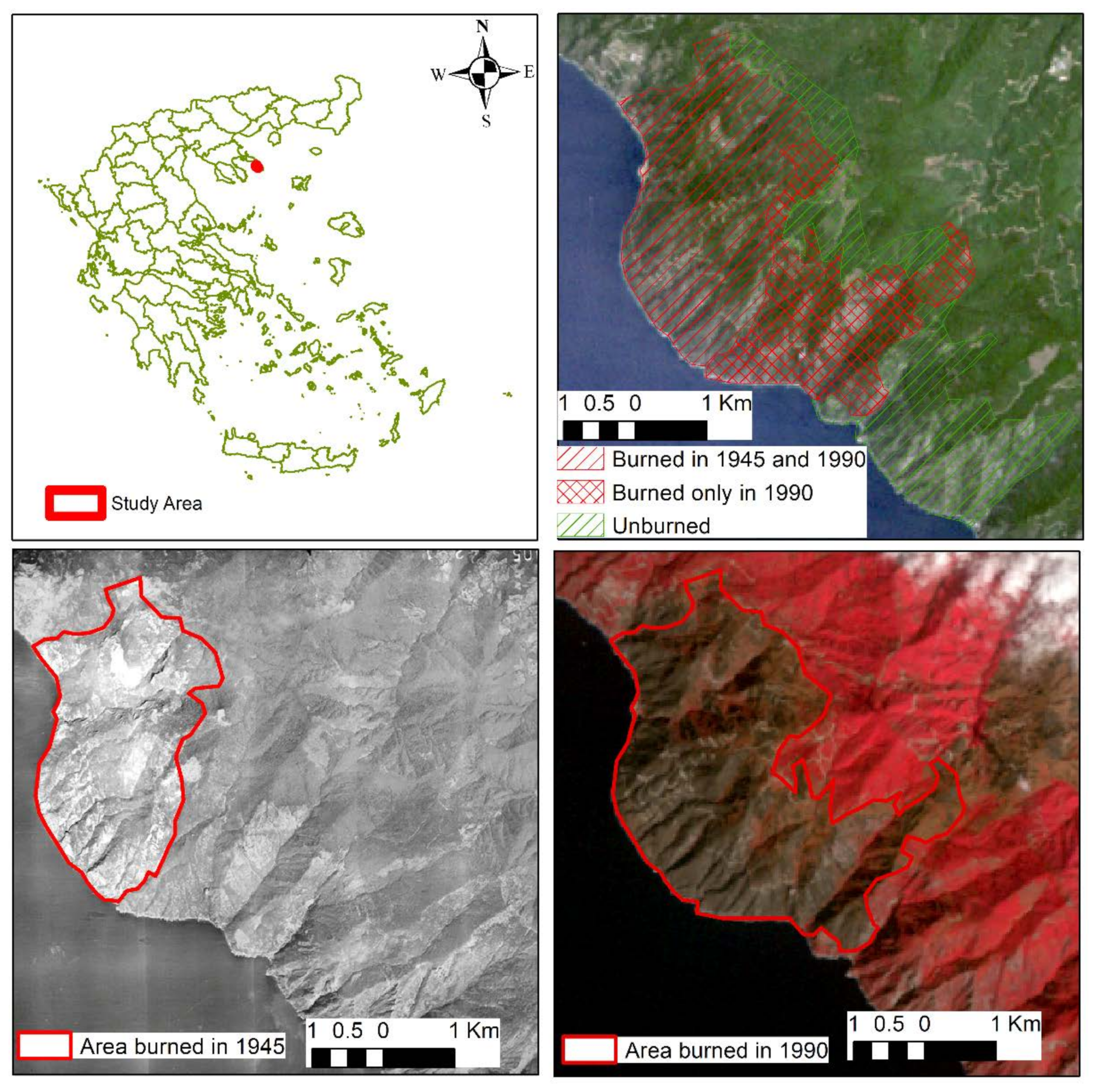
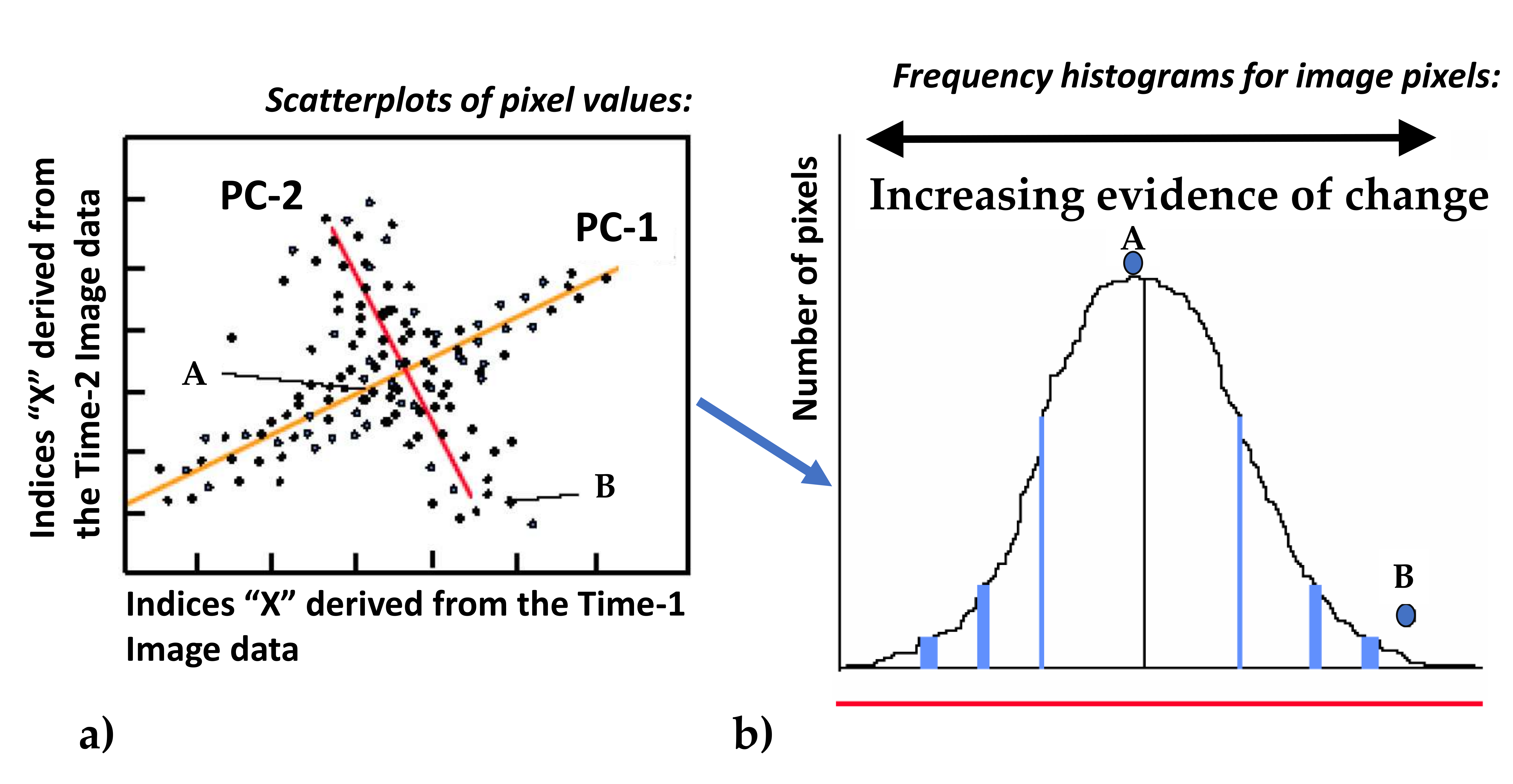
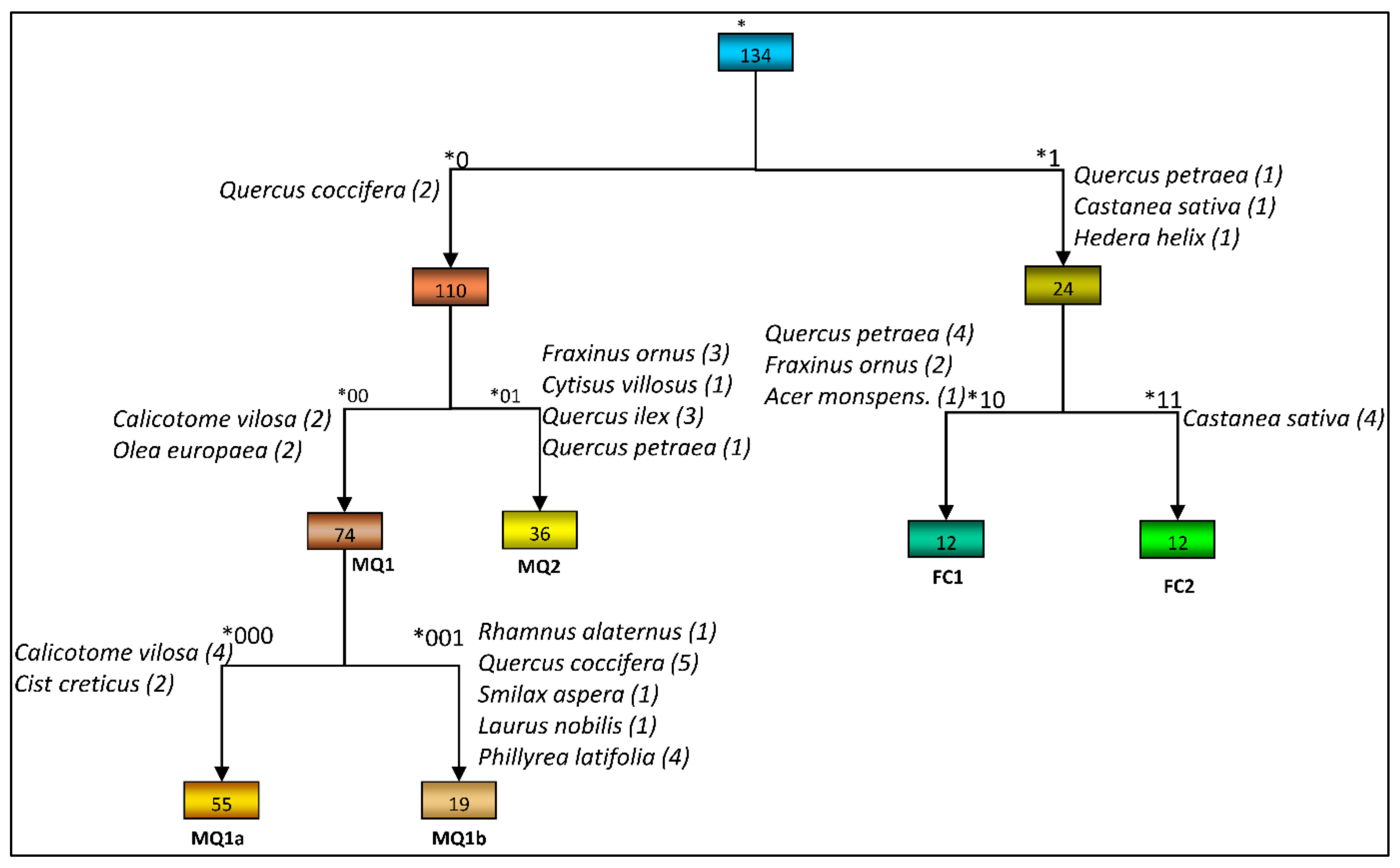
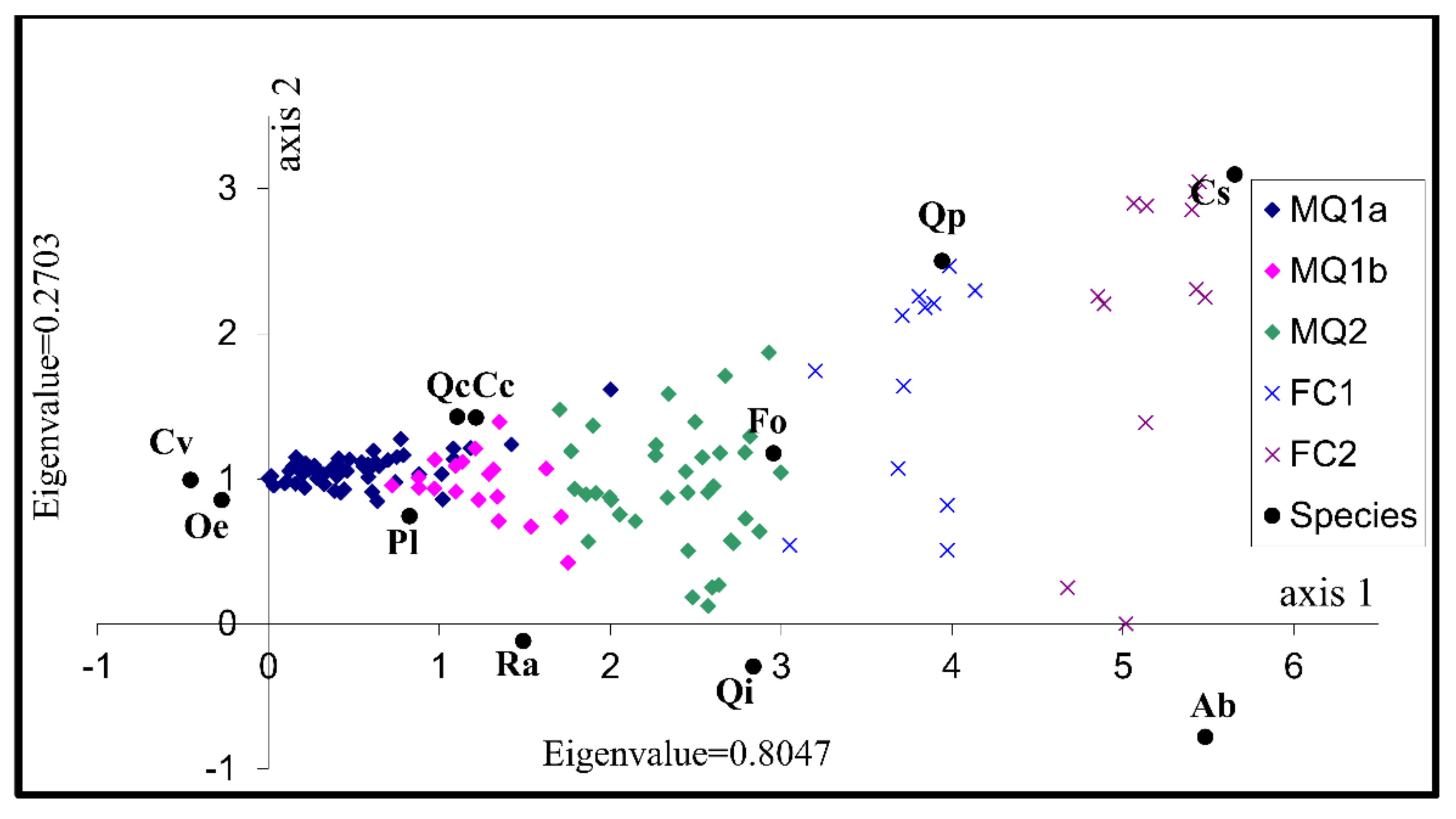
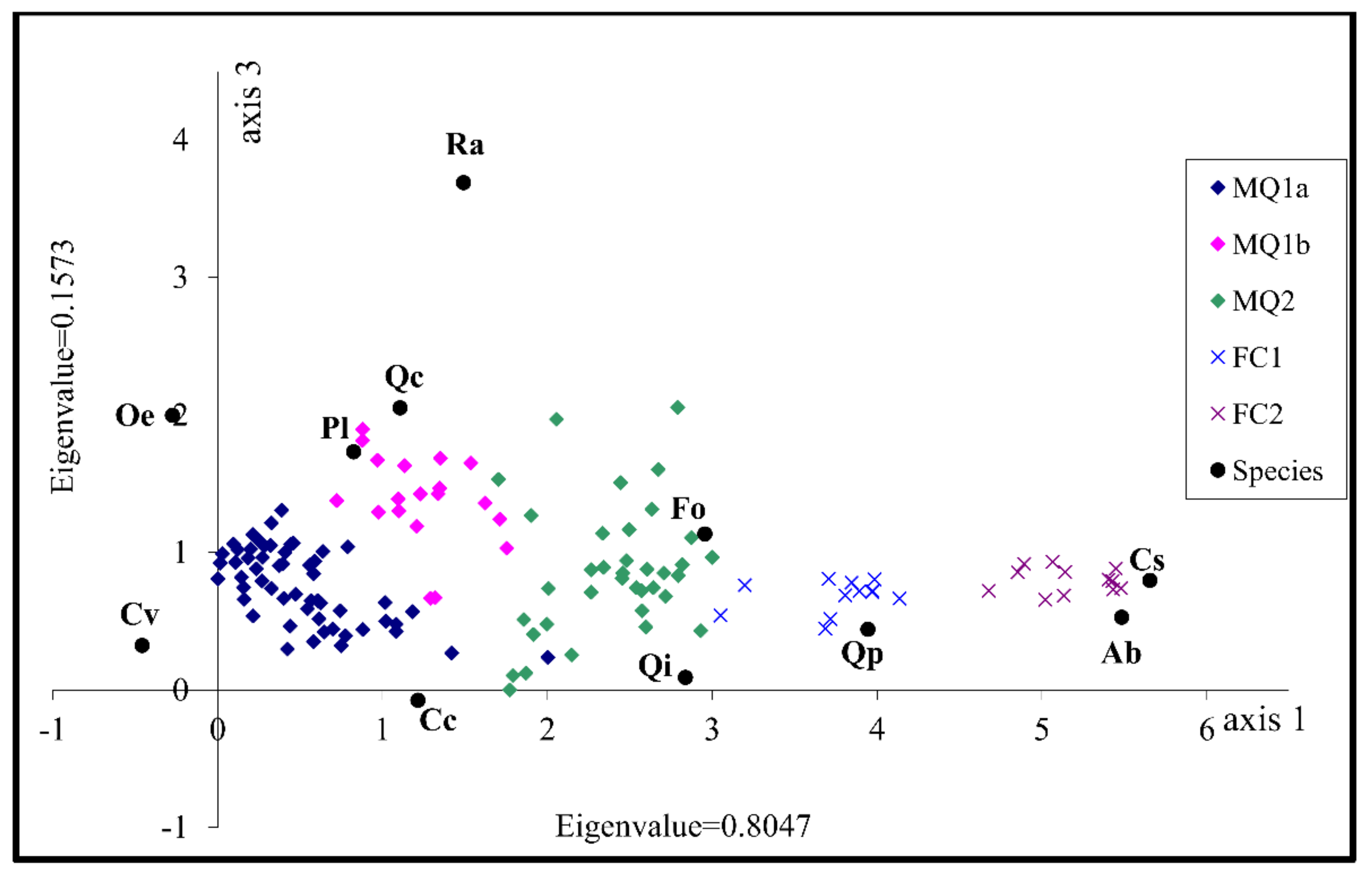
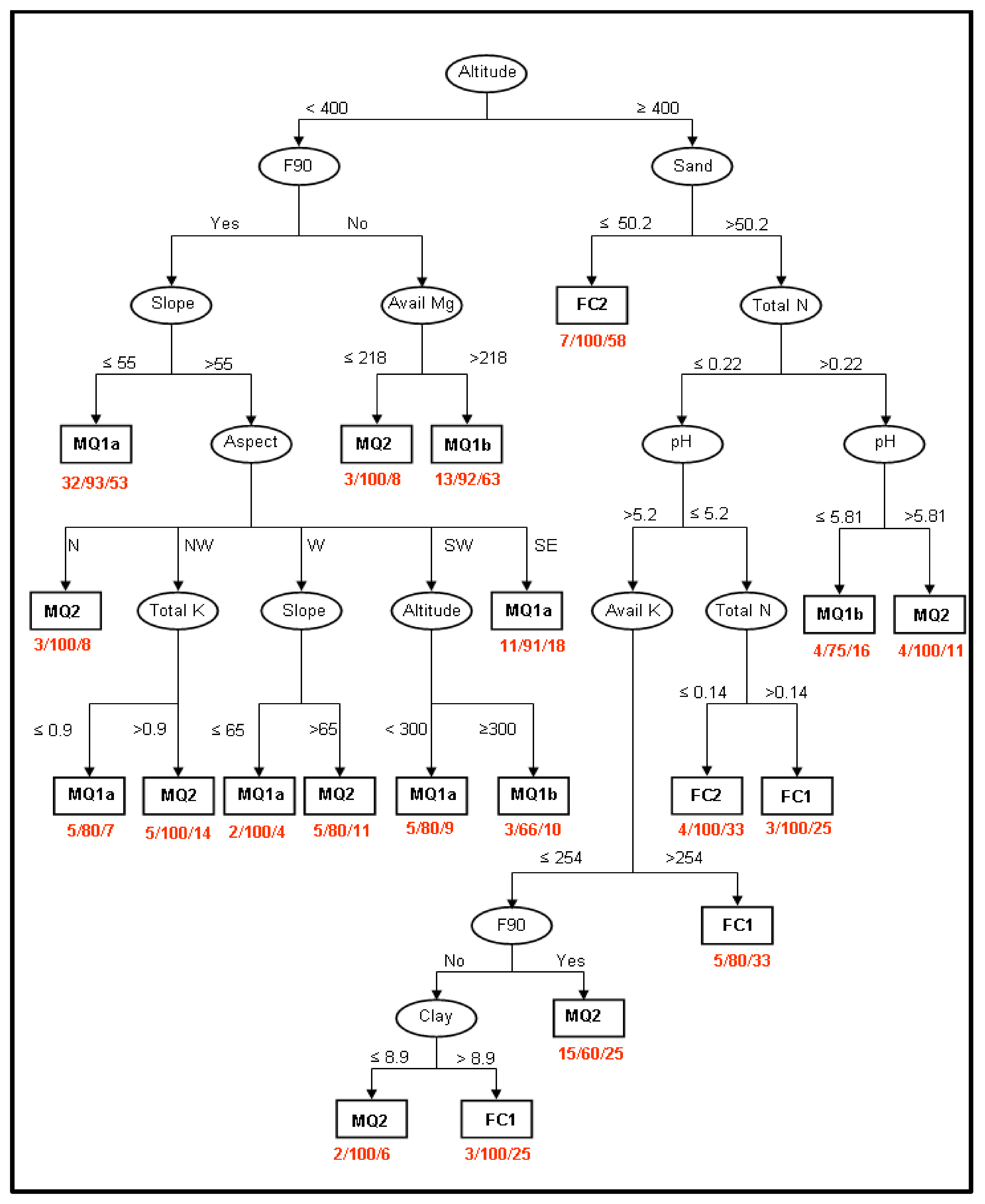
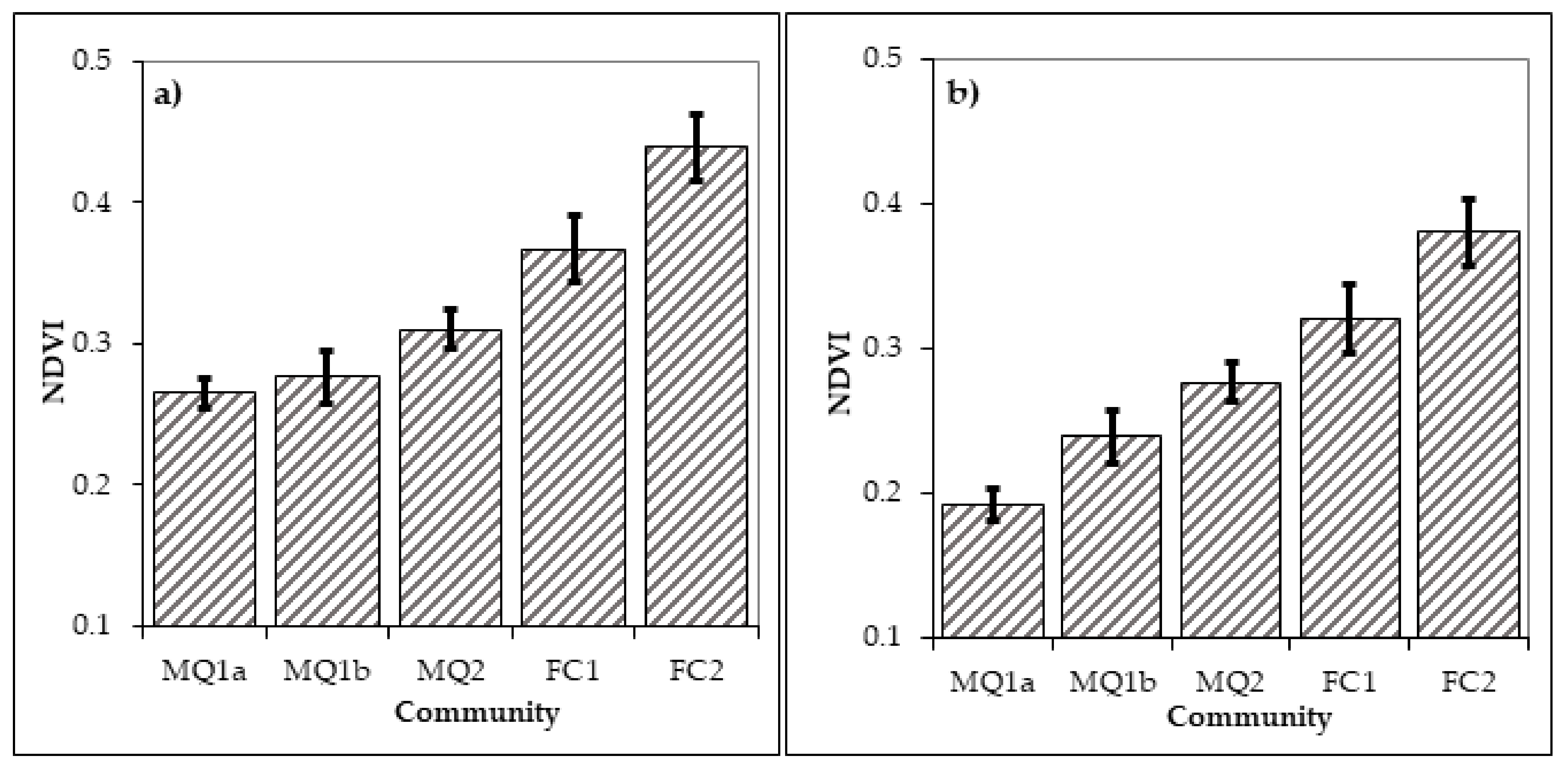
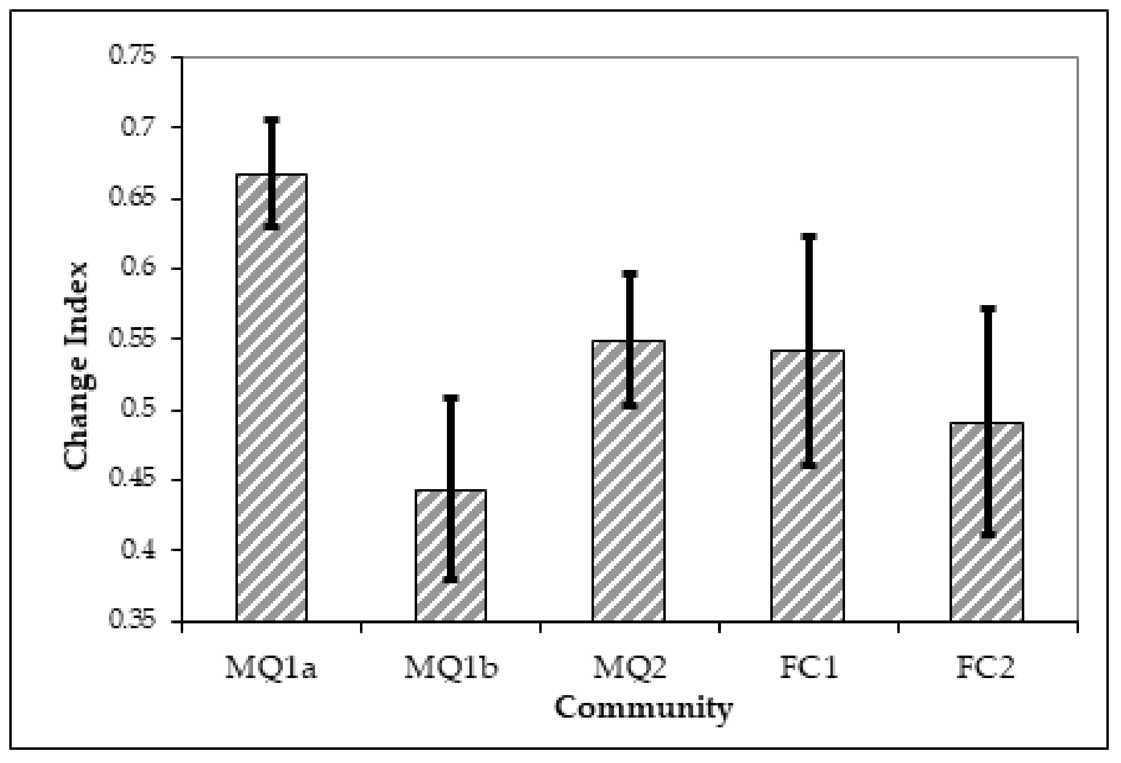
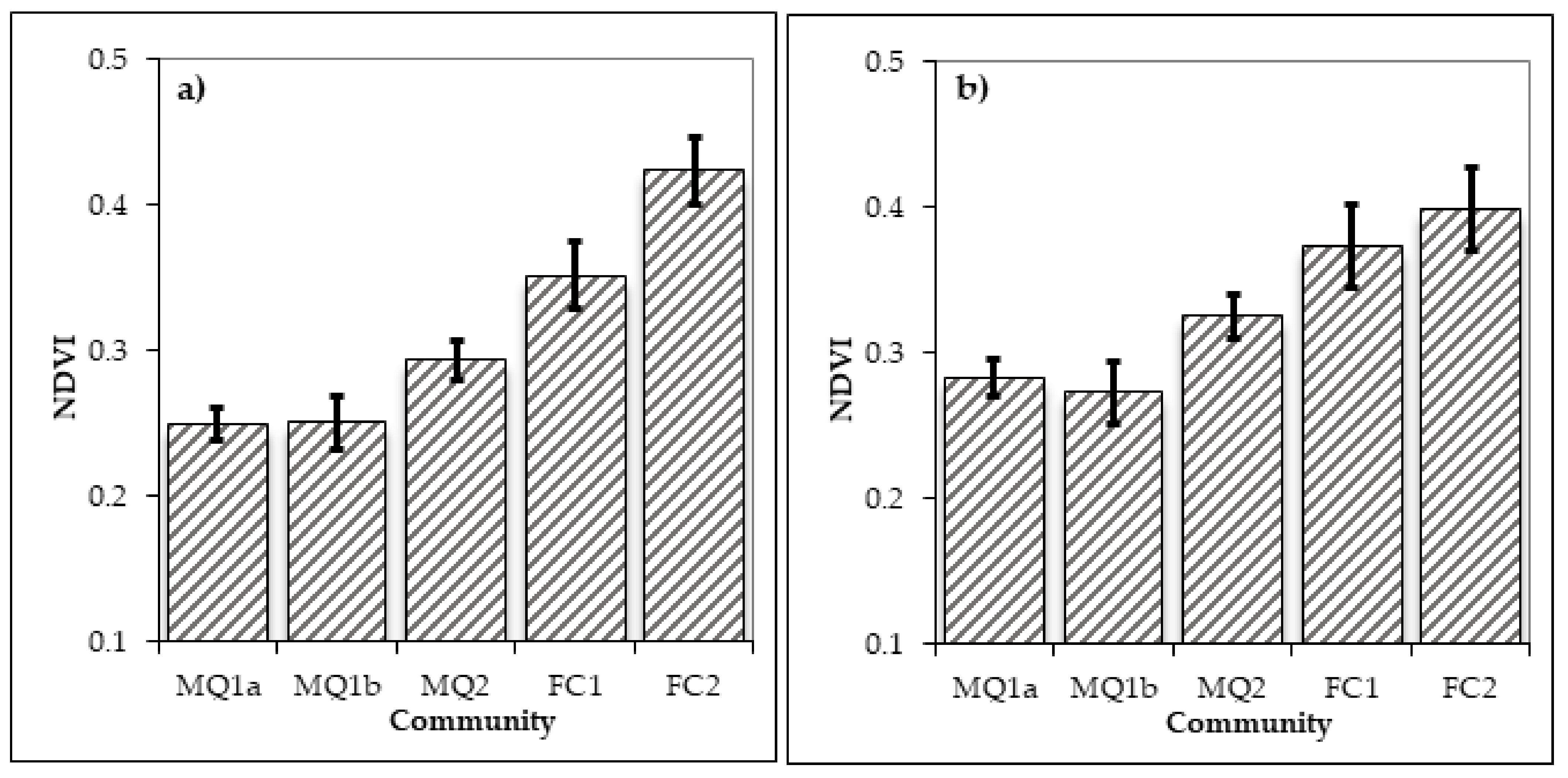
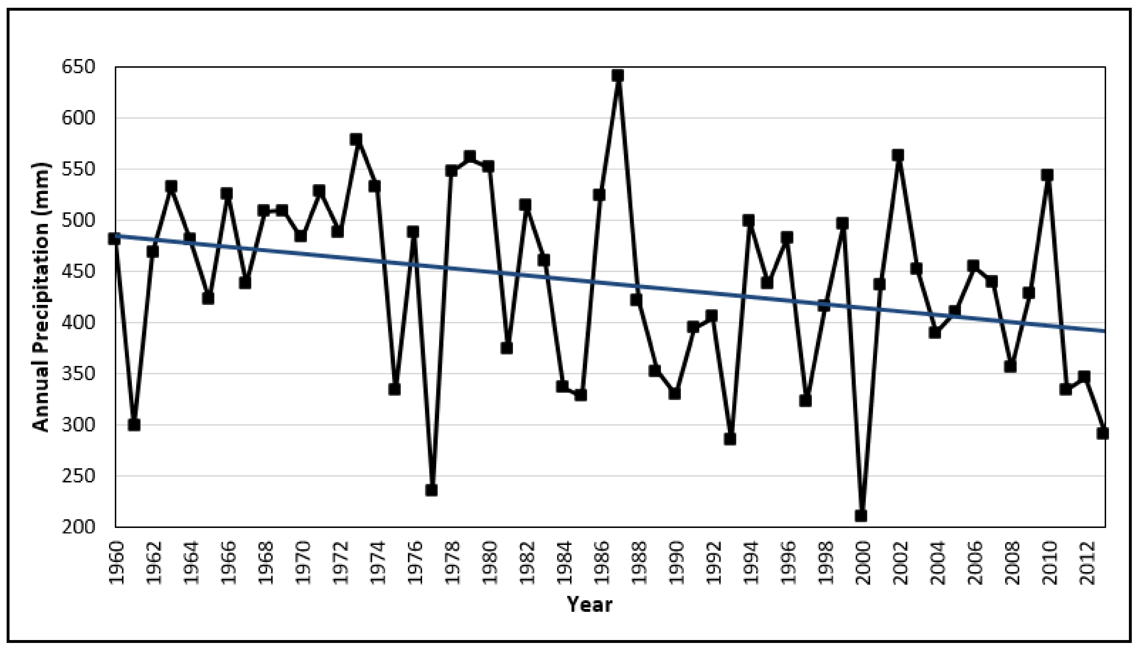
Table 1.
Spectral and Spatial characteristics of the Landsat images used in this study.
| Bands (Wavelength μm)-Spatial Resolution | ||
|---|---|---|
| Landsat 4-TM | Landsat 7-ETM | Landsat 8-OLI |
| B1-Coastal/Aerosol (0.435–0.451)–30 m | ||
| B1-Blue (0.45–0.52)–30 m | B1-Blue (0.441–0.514)–30 m | B2-Blue (0.452–0.512)–30 m |
| B2-Green (0.52–0.60)–30 m | B2-Green (0.519–0.601)–30 m | B3-Green (0.533–0.590)–30 m |
| B3- Red (0.63–0.69)–30 m | B3- Red (0.631–0.692)–30 m | B4- Red (0.636–0.673)–30 m |
| B4-NIR (0.76–0.90)–30 m | B4-NIR (0.772–0.898)–30 m | B5-NIR (0.851–0.879)–30 m |
| B5-SWIR 1 (1.55–1.75)—30 m | B5-SWIR 1 (1.547–1.749)–30 m | B6-SWIR 1 (1.566–1.651)–30 m |
| B7-SWIR 2 (2.08–2.35)–30 m | B7-SWIR 2 (2.064–2.345)–30 m | B7-SWIR 2 (2.107–2.294)–30 m |
| B6-TIR (10.40–12.50)–120 m | B6-TIR (10.31–12.36)–60 m | B10-TIR 1 (10.60–11.19)–30 m |
| B11-TIR 2 (11.50–12.51)–30 m | ||
| B9-Cirrus (1.363–1.384)–30 m | ||
| B8-Pan (0.515–0.896)–15 m | B8-Pan (0.503–0.676)–15 m | |
Table 2.
Species frequencies and abundance range for the groups identified to form communities or sub-communities. Only the constant and frequent species of each group are shown. For the explanation of frequencies and abundance symbols see Section 2.3.
Table 2.
Species frequencies and abundance range for the groups identified to form communities or sub-communities. Only the constant and frequent species of each group are shown. For the explanation of frequencies and abundance symbols see Section 2.3.
| Species | Group *000 n = 55 | Group *001 n = 19 | Group *00 n = 55 + 19 = 74 | Group *01 n = 36 | Group *10 n = 12 | Group *11 n = 12 | Total n = 134 |
|---|---|---|---|---|---|---|---|
| Quercus coccifera | V (2–5) | V (2–6) | V (2–6) | V (1–6) | III (1) | V | |
| Phillyrea latifolia | V (1–5) | V (1–6) | V (1–6) | V (1–4) | V | ||
| Ruscus aculeatus | IV (1–2) | V (1–2) | IV (1–2) | V (1–2) | V (1–2) | V (1–2) | V |
| Olea europaea | V (1–5) | IV (1–3) | V (1–5) | IV | |||
| Fraxinus ornus | III (1–2) | IV (1–2) | III (1–2) | V (1–5) | V (1–3) | III (1–2) | IV |
| Cistus creticus | V (1–4) | V (1–3) | V (1–4) | IV (1–4) | III (1–2) | IV | |
| Arbutus unedo. | IV (1–3) | IV (1–3) | IV (1–3) | IV (1–3) | IV | ||
| Asparagus acutifolious | V (1–2) | V (1–2) | V (1–2) | V (1–2) | IV | ||
| Calicotome villosa | V (2–6) | IV (1–4) | V (1–6) | III | |||
| Quercus ilex | IV (1–5) | V (1–6) | V (1–6) | III (1–3) | III | ||
| Erica arborea | III (1–4) | IV (1–3) | III (1–4) | III (1–3) | III | ||
| Spartium junceum | V (1–6) | IV (1–5) | V (1–6) | III (1–6) | III | ||
| Pistacia terebinthus | III (1–2) | IV (1–2) | IV (1–2) | III | |||
| Cytisus villosus | V (1–5) | V (1–3) | V (1–5) | III | |||
| Laurus nobilis | III (1–3) | IV (1–5) | II | ||||
| Rhamnus alaternus L. | IV (1–3) | II | |||||
| Osyris alba L. | III (1–2) | III (1–3) | III (1–3) | II | |||
| Smilax aspera | IV (1–5) | III (1–5) | II | ||||
| Lonicera implexa Aiton. | III (1) | III (1) | II | ||||
| Quercus petraea | III (1–6) | V (2–6) | V (1–3) | II | |||
| Sorbus domestica L. | III (1) | I | |||||
| Rubus sp L. | III (1) | III (1) | I | ||||
| Hedera helix L. | IV (1) | V (1–2) | I | ||||
| Acer monspessulanum L. | IV (1–2) | I | |||||
| Abies borisii–regis | III (1–2) | IV (1–6) | I | ||||
| Sorbus torminalis (L.) Crantz | III (1) | I | |||||
| Castanea sativa | IV (2–3) | V (3–6) | I | ||||
| Ruscus hypoglossum | IV (1–2) | I | |||||
| Ilex aquifolium L. | III (1–2) | III (1–2) | I | ||||
| Quercus frainetto | III (2–6) | I | |||||
| Genista tinctoria L. | V (1–3) | III (1–3) | I | ||||
| Rosa sp L. | III (1) | I | |||||
| Comm. Codenames 1 | MQ1a | MQ1b | MQ1 | MQ2 | FC1 | FC2 |
1 Codenames were given to the communities and sub-communities resulting by the interpretation of the classification results for convenience in the description and further analysis (see Section 3.1 for full community names).
Table 3.
Summary of DCA results for all samples and all species.
| Axes | 1 | 2 | 3 | 4 | Total Inertia |
|---|---|---|---|---|---|
| Eigenvalues: | 0.805 | 0.270 | 0.157 | 0.121 | 3.865 |
| Cumulative percentage variance of species data: | 20.8 | 27.8 | 31.9 | 35.0 | |
| Sum of all eigenvalues | 3.865 |
Table 4.
Mean (Mn), Standard Deviation (SD) and Median (Md) cover for all constant and frequent species in each community and sub-community.
Table 4.
Mean (Mn), Standard Deviation (SD) and Median (Md) cover for all constant and frequent species in each community and sub-community.
| Species | MQ1a | MQ1b | MQ2 | FC1 | FC2 | ||||||||||
|---|---|---|---|---|---|---|---|---|---|---|---|---|---|---|---|
| Mn | SD | Md | Mn | SD | Md | Mn | SD | Md | Mn | SD | Md | Mn | SD | Md | |
| Quercus coccifera | 19.0 | 7.5 | 20.5 | 41.0 | 17.6 | 37.0 | 13.9 | 16.1 | 9.2 | 1.5 | 3.5 | 0.3 | 0.1 | 0.4 | 0.0 |
| Phillyrea latifolia | 12.7 | 8.2 | 12.4 | 25.4 | 17.4 | 30.9 | 6.9 | 6.3 | 5.4 | 0.7 | 1.3 | 0.0 | 0.0 | 0.0 | 0.0 |
| Ruscus aculeatus | 0.9 | 1.2 | 0.6 | 2.7 | 1.6 | 2.6 | 3.7 | 2.5 | 4.3 | 2.9 | 1.7 | 3.5 | 1.6 | 1.6 | 1.4 |
| Olea europaea | 7.1 | 7.9 | 4.3 | 7.1 | 7.0 | 6.5 | 0.2 | 0.5 | 0.0 | 0.0 | 0.0 | 0.0 | 0.0 | 0.0 | 0.0 |
| Fraxinus ornus | 1.6 | 2.8 | 0.0 | 3.8 | 3.8 | 2.6 | 18.4 | 9.6 | 20.5 | 14.9 | 7.1 | 14.3 | 1.4 | 2.8 | 0.0 |
| Cistus creticus | 10.0 | 8.4 | 9.2 | 3.4 | 3.7 | 1.4 | 6.6 | 7.6 | 3.5 | 0.9 | 1.8 | 0.3 | 0.0 | 0.0 | 0.0 |
| Arbutus unedo | 2.2 | 3.2 | 0.6 | 2.4 | 3.5 | 1.4 | 4.6 | 5.6 | 2.0 | 0.1 | 0.2 | 0.0 | 0.0 | 0.0 | 0.0 |
| Asparagus acutifolious | 1.4 | 1.3 | 0.6 | 1.8 | 1.3 | 1.4 | 2.0 | 1.9 | 1.4 | 0.4 | 0.7 | 0.1 | 0.0 | 0.0 | 0.0 |
| Calicotome villosa | 48.0 | 16.0 | 51.0 | 5.0 | 7.5 | 1.4 | 0.8 | 3.1 | 0.0 | 0.0 | 0.0 | 0.0 | 0.0 | 0.0 | 0.0 |
| Quercus ilex | 1.1 | 2.4 | 0.0 | 7.5 | 10.8 | 2.6 | 29.8 | 22.0 | 28.2 | 16.6 | 22.2 | 6.8 | 1.4 | 3.5 | 0.1 |
| Erica arborea | 2.6 | 4.9 | 0.0 | 4.0 | 5.5 | 1.4 | 2.0 | 4.0 | 0.3 | 0.3 | 0.8 | 0.0 | 0.0 | 0.0 | 0.0 |
| Spartium junceum | 10.9 | 13.3 | 4.3 | 6.8 | 11.9 | 1.4 | 11.2 | 15.9 | 1.4 | 0.4 | 1.2 | 0.0 | 0.0 | 0.0 | 0.0 |
| Pistacia terebinthus | 0.8 | 1.5 | 0.1 | 1.3 | 1.4 | 0.6 | 0.3 | 0.6 | 0.0 | 0.0 | 0.0 | 0.0 | 0.0 | 0.0 | 0.0 |
| Cytisus villosus | 0.0 | 0.0 | 0.0 | 0.3 | 1.0 | 0.0 | 14.5 | 13.3 | 12.4 | 6.0 | 6.4 | 4.3 | 13.3 | 13.8 | 9.2 |
| Laurus nobilis | 0.3 | 1.2 | 0.0 | 1.8 | 3.4 | 0.1 | 7.5 | 10.6 | 1.4 | 0.1 | 0.2 | 0.0 | 0.0 | 0.0 | 0.0 |
| Rhamnus alaternus | 0.0 | 0.1 | 0.0 | 2.1 | 3.8 | 0.6 | 0.5 | 1.3 | 0.0 | 0.0 | 0.0 | 0.0 | 0.0 | 0.0 | 0.0 |
| Osyris alba | 0.8 | 1.2 | 0.0 | 1.4 | 3.0 | 0.0 | 0.6 | 1.7 | 0.0 | 0.0 | 0.0 | 0.0 | 0.0 | 0.0 | 0.0 |
| Smilax aspera | 1.2 | 4.4 | 0.0 | 3.7 | 9.9 | 1.4 | 7.3 | 13.3 | 0.0 | 0.0 | 0.0 | 0.0 | 0.0 | 0.0 | 0.0 |
| Euphorbia characias | 0.6 | 0.8 | 0.0 | 0.3 | 0.5 | 0.0 | 0.3 | 0.5 | 0.0 | 0.0 | 0.0 | 0.0 | 0.0 | 0.0 | 0.0 |
| Lonicera implexa | 0.3 | 0.9 | 0.0 | 0.3 | 0.4 | 0.0 | 0.5 | 0.6 | 0.6 | 0.2 | 0.3 | 0.0 | 0.0 | 0.0 | 0.0 |
| Quercus petraea | 0.5 | 3.4 | 0.0 | 0.2 | 1.0 | 0.0 | 7.9 | 13.0 | 2.6 | 53.4 | 25.5 | 58.9 | 7.1 | 5.2 | 7.9 |
| Sorbus domestica | 0.0 | 0.0 | 0.0 | 0.0 | 0.0 | 0.0 | 0.9 | 3.5 | 0.0 | 1.1 | 3.6 | 0.0 | 0.2 | 0.3 | 0.0 |
| Rubus sp | 0.0 | 0.0 | 0.0 | 0.0 | 0.0 | 0.0 | 0.4 | 1.6 | 0.0 | 1.2 | 1.4 | 1.0 | 0.4 | 0.7 | 0.0 |
| Hedera helix | 0.0 | 0.0 | 0.0 | 0.0 | 0.0 | 0.0 | 0.1 | 0.3 | 0.0 | 0.8 | 1.0 | 0.6 | 2.9 | 1.9 | 2.6 |
| Acer monspessulanum | 0.0 | 0.0 | 0.0 | 0.0 | 0.0 | 0.0 | 0.8 | 1.9 | 0.0 | 1.3 | 1.6 | 0.6 | 0.0 | 0.0 | 0.0 |
| Abies borisii-regis | 0.0 | 0.0 | 0.0 | 0.0 | 0.0 | 0.0 | 0.0 | 0.2 | 0.0 | 1.0 | 1.7 | 0.0 | 15.9 | 20.1 | 3.5 |
| Sorbus torminalis | 0.0 | 0.0 | 0.0 | 0.0 | 0.0 | 0.0 | 0.0 | 0.2 | 0.0 | 0.4 | 0.5 | 0.0 | 0.1 | 0.2 | 0.0 |
| Castanea sativa | 0.0 | 0.0 | 0.0 | 0.0 | 0.0 | 0.0 | 0.0 | 0.0 | 0.0 | 7.0 | 5.4 | 7.9 | 74.9 | 31.5 | 97.3 |
| Ruscus hypoglossum | 0.0 | 0.0 | 0.0 | 0.0 | 0.0 | 0.0 | 0.0 | 0.0 | 0.0 | 0.2 | 0.3 | 0.0 | 1.0 | 1.3 | 0.6 |
| Ilex aquifolium | 0.0 | 0.0 | 0.0 | 0.0 | 0.0 | 0.0 | 0.0 | 0.0 | 0.0 | 1.5 | 2.6 | 0.7 | 1.4 | 2.6 | 0.6 |
| Quercus frainetto | 0.0 | 0.0 | 0.0 | 0.0 | 0.0 | 0.0 | 0.0 | 0.0 | 0.0 | 7.9 | 18.5 | 0.0 | 13.3 | 19.9 | 0.0 |
| Genista trinctoria | 0.0 | 0.0 | 0.0 | 0.0 | 0.0 | 0.0 | 0.2 | 0.5 | 0.0 | 4.3 | 6.8 | 1.4 | 2.1 | 3.8 | 0.3 |
| Rosa sp | 0.0 | 0.0 | 0.0 | 0.0 | 0.0 | 0.0 | 0.0 | 0.0 | 0.0 | 0.2 | 0.3 | 0.0 | 0.1 | 0.2 | 0.0 |
Table 5.
Post Hoc pair-wise comparisons on the NDVI differences between the communities for August 2001 and June 1989. ns = Not significant, * = Significant, ** = Very significant, *** = Extremely significant.
Table 5.
Post Hoc pair-wise comparisons on the NDVI differences between the communities for August 2001 and June 1989. ns = Not significant, * = Significant, ** = Very significant, *** = Extremely significant.
| 1989 | 2001 | |||||||
|---|---|---|---|---|---|---|---|---|
| Community | MQ1a | MQ1b | MQ2 | FC1 | MQ1a | MQ1b | MQ2 | FC1 |
| MQ1b | 0.84 ns | <0.001 *** | ||||||
| MQ2 | <0.001 *** | 0.032 * | <0.001 *** | 0.012 * | ||||
| FC1 | <0.001 *** | <0.001 *** | <0.001 *** | <0.001 *** | <0.001 *** | 0.009 ** | ||
| FC2 | <0.001 *** | <0.001 *** | <0.001 *** | <0.001 *** | <0.001 *** | <0.001 *** | <0.001 *** | 0.003 ** |
Table 6.
Post Hoc pair-wise comparisons on the Change Index values between the communities 1989–2001. ns = Not significant, * = Significant, *** = Extremely significant.
Table 6.
Post Hoc pair-wise comparisons on the Change Index values between the communities 1989–2001. ns = Not significant, * = Significant, *** = Extremely significant.
| Community | MQ1a | MQ1b | MQ2 | FC1 |
|---|---|---|---|---|
| MQ1b | <0.001 *** | |||
| MQ2 | <0.001 *** | 0.066 ns | ||
| FC1 | <0.043 * | 0.324 ns | 0.999 ns | |
| FC2 | <0.001 *** | 0.893 ns | 0.737 ns | 0.904 ns |
Table 7.
Post Hoc pair-wise comparisons on the NDVI differences between the communities for August 2011 and July 2021. ns = Not significant, * = Significant, ** = Very significant, *** = Extremely significant.
Table 7.
Post Hoc pair-wise comparisons on the NDVI differences between the communities for August 2011 and July 2021. ns = Not significant, * = Significant, ** = Very significant, *** = Extremely significant.
| 2011 | 2021 | |||||||
|---|---|---|---|---|---|---|---|---|
| Community | MQ1a | MQ1b | MQ2 | FC1 | MQ1a | MQ1b | MQ2 | FC1 |
| MQ1b | 1 ns | 0.907 ns | ||||||
| MQ2 | <0.001 *** | 0.020 * | <0.001 *** | 0.001 ** | ||||
| FC1 | <0.001 *** | <0.001 *** | 0.009 ** | <0.001 *** | <0.001 *** | 0.029 * | ||
| FC2 | <0.001 *** | <0.001 *** | <0.001 *** | 0.010 ** | <0.001 *** | <0.001 *** | <0.001 *** | 0.741 ns |
Table 8.
Mean annual precipitation and temperature values reported in studies of Q. coccifera recovery after fire in the western Mediterranean.
Table 8.
Mean annual precipitation and temperature values reported in studies of Q. coccifera recovery after fire in the western Mediterranean.
| Country | Mean Annual Precipitation (mm) | Mean Annual Temperature (°C) |
|---|---|---|
| France (Trabaud, 1990) | 800–1000 | - |
| France (Trabaud & Lepart, 1981) | 1100 | 14.4 |
| France (Trabaud, 1991) | 919 | 13.2 |
| France (Malanson & Trabaud, 1988) | 980 | - |
| Spain (Delitti et al., 2005) | 600 | 14 |
| Spain (Lloret & Vila, 1997) | 591 | - |
| Portugal (Clemente et al., 1996) | 1080 | - |
| Current Study | 470 | 15.7 |
Publisher’s Note: MDPI stays neutral with regard to jurisdictional claims in published maps and institutional affiliations. |
© 2021 by the authors. Licensee MDPI, Basel, Switzerland. This article is an open access article distributed under the terms and conditions of the Creative Commons Attribution (CC BY) license (https://creativecommons.org/licenses/by/4.0/).
Share and Cite
MDPI and ACS Style
Xofis, P.; Buckley, P.G.; Takos, I.; Mitchley, J. Long Term Post-Fire Vegetation Dynamics in North-East Mediterranean Ecosystems. The Case of Mount Athos Greece. Fire 2021, 4, 92. https://0-doi-org.brum.beds.ac.uk/10.3390/fire4040092
AMA Style
Xofis P, Buckley PG, Takos I, Mitchley J. Long Term Post-Fire Vegetation Dynamics in North-East Mediterranean Ecosystems. The Case of Mount Athos Greece. Fire. 2021; 4(4):92. https://0-doi-org.brum.beds.ac.uk/10.3390/fire4040092
Chicago/Turabian StyleXofis, Panteleimon, Peter G. Buckley, Ioannis Takos, and Jonathan Mitchley. 2021. "Long Term Post-Fire Vegetation Dynamics in North-East Mediterranean Ecosystems. The Case of Mount Athos Greece" Fire 4, no. 4: 92. https://0-doi-org.brum.beds.ac.uk/10.3390/fire4040092