A Comparison of Time-Frequency Methods for Real-Time Application to High-Rate Dynamic Systems


1
Department of Civil, Construction, and Environmental Engineering, Iowa State University, Ames, IA 50010, USA
2
Department of Civil and Environmental Engineering, Western University, London, ON N6A 3K7, Canada Canada
3
Air Force Research Laboratory, Eglin AFB, FL 32542, USA
*
Author to whom correspondence should be addressed.
Vibration 2020, 3(3), 204-216; https://0-doi-org.brum.beds.ac.uk/10.3390/vibration3030016
Submission received: 24 July 2020
/
Accepted: 21 August 2020
/
Published: 24 August 2020
(This article belongs to the Special Issue Inverse Dynamics Problems)
Abstract
:High-rate dynamic systems are defined as engineering systems experiencing dynamic events of typical amplitudes higher than 100 g for a duration of less than 100 ms. The implementation of feedback decision mechanisms in high-rate systems could improve their operations and safety, and even be critical to their deployment. However, these systems are characterized by large uncertainties, high non-stationarities, and unmodeled dynamics, and it follows that the design of real-time state-estimators for such purpose is difficult. In this paper, we compare the promise of five time-frequency representation (TFR) methods at conducting real-time state estimation for high-rate systems, with the objective of providing a path to designing implementable algorithms. In particular, we examine the performance of the short-time Fourier transform (STFT), wavelet transformation (WT), Wigner–Ville distribution (WVD), synchrosqueezed transform (SST), and multi-synchrosqueezed transform (MSST) methods. This study is conducted using experimental data from the DROPBEAR (Dynamic Reproduction of Projectiles in Ballistic Environments for Advanced Research) testbed, consisting of a rapidly moving cart on a cantilever beam that acts as a moving boundary condition. The capability of each method at extracting the beam’s fundamental frequency is evaluated in terms of precision, spectral energy concentration, computation speed, and convergence speed. It is found that both the STFT and WT methods are promising methods due to their fast computation speed, with the WT showing particular promise due to its faster convergence, but at the cost of lower precision on the estimation depending on circumstances.
1. Introduction
High-rate dynamic systems are defined as engineering systems experiencing high-amplitude disruptions (acceleration >100 g) within a very short duration (<100 ms) [1]. Examples of high-rate systems include blast mitigation mechanisms, hypersonic aircraft, and advanced weaponry. Generally, these systems experience rapid changes in their dynamics that can cause malfunctions and sudden failures. The capability to conduct real-time identification of such changes combined with real-time adaptation is critical in ensuring their continuous operation and safety [2]. In terms of system identification, the high-rate problem consists of being able to identify and quantify changes in dynamics over a very short period of time for dynamics containing (1) large uncertainties in the external loads; (2) high levels of non-stationarities and heavy disturbance, and (3) unmodeled dynamics from changes in system configuration.
Work directly addressing the problem of high-rate state estimation, or system identification is limited. In previous work, the authors have proposed an adaptive sequential neural network with a self-adapting input space enabling fast learning of nonstationary signals from high-rate systems [3]. Although the data-based technique showed great promise at high rate state estimation, it did not provide insight into the system’s physical characteristics, as it is generally the case with data-based techniques. Physics-driven methods, such as those borrowing on model reference adaptive system (MRAS) theory, showed great promise in handling nonlinearities, uncertainties, and perturbations [4,5]. MRAS was applied to the problem of high-rate state estimation in [6], where the position of a moving cart was accurately identified under 172 ms through a time-based adaptive algorithm used in reaching the reference model with an average computing time of 93 per step, obtained through numerical simulations conducted in MATLAB. A frequency-based approach was proposed in [7] to identify the position of that same cart. Their algorithm consisted of extracting the dominating frequency through a Fourier transform over a finite set of data and matching that frequency to a set of pre-analyzed finite element models. The authors applied their algorithm experimentally using a field-programmable gate array (FPGA), and were able to accurately identify the position of the cart within 202 ms with a 4.04 ms processing time per step.
A net advantage of frequency-based methods over time-based methods is that they do not typically rely on the tuning of parameters such as adaptive gains. However, they are harder to apply in real time because they are inherently batch processing techniques. It follows that, to enable applications to high-rate systems, one must integrate a temporal approach to the frequency technique in order to extract the required real-time information, a method known as time-frequency representation (TFR). For example, this was done in [7] through the use of a non-overlapping sliding window of 198 ms length. The objective of this paper is to explore the applicability of TFRs to the high-rate problem.
TFRs are widely used for the detection and quantification of faults through vibration-based data [8]. Frequency domain characteristics, such as frequencies, damping ratios, energy in different frequency ranges, and time-frequency domain characteristics, such as time-frequency spread [9], can be used as key features to conduct structural health monitoring [9]. A number of TFRs for instant frequency recognition have been proposed. Popular approaches include linear non-parametric methods, such as short-time Fourier transform (STFT), wavelet transform (WT), and Wigner–Ville distribution (WVD) [9,10]. The application of these methods results in a trade-off between time and frequency resolutions [11]. An adaptive non-parametric method have also been proposed, including the Hilbert–Huang transform (HHT) [12,13,14], the Cauchy continuous wavelet transform (CCWT) [15], the instantaneous frequencies (IF) re-assignment methods, synchrosqueezing transform (SST) [16], and the multi-SST (MSST) [17].
In this paper, five of these methods are selected, namely the STFT, WT, WVD, SST, and MSST, and their real-time applicability are compared with a specific focus on weakly time-varying systems, here defined as systems with continuously time-varying frequencies, in opposition to abrupt changes (steps, jumps, shifts) in frequencies [18,19]. The objective is to provide a path in designing the next generation of real-time high-rate algorithms. The quantification of performance is conducted on experimental data from the DROPBEAR (Dynamic Reproduction of Projectiles in Ballistic Environments for Advanced Research) testbed [20], which includes the moving cart dynamics used in [6,7]. The remainder of the paper is organized as follows. First, the background on the five TFR methods is presented—after DROPBEAR is introduced and the performance of the methods is analyzed numerically on two different sets of experimental data. Lastly, the performance of each method is compared, and key conclusions are drawn.
2. Time-Frequency Response Methods
This section gives an introductory background on the TFR methods under comparison. These include the following traditional TFR methods: STFT, WT, WVD, and TF re-assignment methods: SST and MSST.
2.1. Traditional TFR Methods
2.1.1. Short-Time Fourier Transform
The Fourier transform of a sequence of an N discretely sampled signal to the discrete frequency domain is taken as:
where j is the imaginary unit, and k is the corresponding frequency. To integrate a temporal notion, the Fourier transform can be applied over short time segments through a moving window, where the signal can be assumed stationary between two consecutive segments, a method known as STFT. The local Fourier spectrum of each segment can be generated around the position of the window, and the frequency’s temporal variation can be observed locally. This is done by modifying Equation (1) as follows [21,22]:
where is the windowing function of length L, and m denotes a time shift. With the STFT, a narrower window will improve the time domain resolution but will result in a lower frequency domain resolution. Conversely, a wider window will improve the frequency domain resolution but will result in a lower time domain resolution.
2.1.2. Wavelet Transform
The WT method is known for its superior spectral resolution by overcoming the STFT’s requirement of predefining a window length. It provides a linear time-frequency representation based on a preselected mother wavelet using simultaneous dilation and translation operations. The discretized version of the continuous WT of a signal is written [23,24]:
where c is scaling factor. Generally, the WT method has better temporal resolution and lower frequency resolution for higher frequency contents, and better frequency resolution and lower temporal resolution for lower frequency contents. The resulting time-frequency signal transform may be blurred and cannot achieve high resolution simultaneously in time and frequency.
2.1.3. Wigner–Ville Distribution
The WVD method is an approach based on the quadratic energy density obtained through an instantaneous autocorrelation function [25]:
where the asterisk denotes the complex conjugate. Challenges in applying the WVD include interferences and negative values [26]. There are times when cross-terms produce oscillatory interference with multiple frequency components, and the magnitude of the interference may range from extremely negative to extremely positive values.
2.2. Time-Frequency Reassignment
2.2.1. Synchrosqueezing Transform
The SST method is time-frequency reallocation method that yields finer time-frequency representations for a non-stationary multi-component signal. With SST, the energies of the time-frequency coefficients are reassigned to achieve higher energy around the trajectories of IF, resulting in more accurate tracking of these IFs [27]. The SST representation is conducted using:
where is the discrete scale for which the wavelet decomposition is computed, and is a scaling step. The SST results in a more concentrated profile and unique IF curves but is inherently more computationally intensive comparing to the WT method. A limitation of the SST method is that it assumes a weakly time-varying system.
2.2.2. Multi-Synchrosqueezing Transform
The MSST method is an improvement of the SST that results in a sharper energy concentration of the TFR [17]. It does not require any other redundant parameter or a priori information to demodulate the frequency-modulated signals, and thus it can be applied beyond weakly time-varying systems. MSST is formulated to post-processes STFT:
Multiple iterations of the process can be conducted with
where is the SST at the iteration for . Increasing N will yield better IF estimates, but at the cost of higher computational time.
3. Methodology
This section introduces the research methodology. It includes a description of the experimental setup, data collection process, and TFR performance investigation methodology.
3.1. Experiment Setup
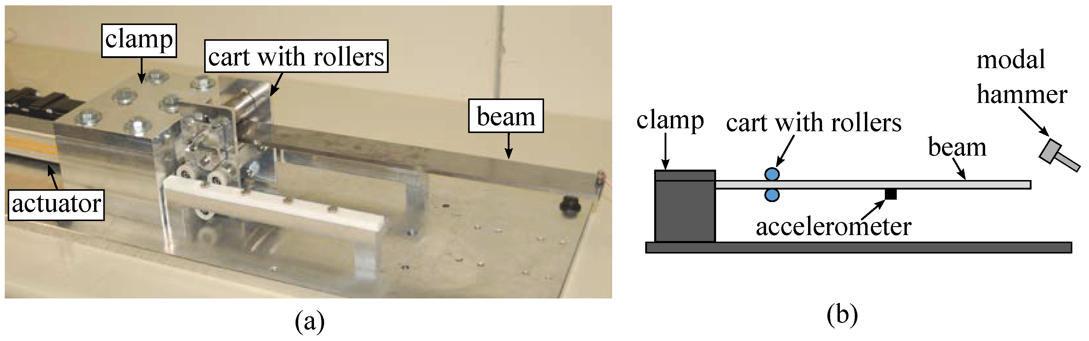
DROPBEAR is an experimental testbed designed to conduct reproducible high-rate dynamic responses [20]. Shown in Figure 1, the testbed features a cantilever steel beam with a rolling cart moving along the beam. The movable cart functions as a variable pin, used to mimic sudden or gradual changes in stiffness due to a change in boundary conditions. The beam was equipped with one PCB 353B17 accelerometer connected to the beam located 300 mm away from the clamp to measure the beam’s response to the moving cart. A modal hammer PCB 086C01 was used to excite the beam at the tip. Figure 1 also shows an electromagnet that can be used to simulate a sudden change in mass through a controlled drop. That feature was not utilized in generating test data used in this paper.
Two types of experiments were conducted. First, the beam was excited with the cart fixed at various locations (i.e., ”fixed cart configuration”): positions A, B, C, D (respectively 50 mm, 100 mm, 150 mm, and 200 mm away from the clamp). For each location, the cart was maintained in place for 2 s and the beam impacted at 0.5, 2.5, 4.5, and 6.5 s (Figure 2a). Data from the accelerometer were sampled at 1 kHz and used to compute frequency response functions (FRFs) using the estimation method [28] plotted in Figure 2c and extract the fundamental natural frequencies at 26.5, 31, 38, and 47.5 Hz (Positions A, B, C, and D, respectively). The fixed cart configuration was used to examine the performance of each TFR method over the entire dataset, without the use of sliding windows (except for the STFT). Second, the cart was moved (i.e., “moving cart configuration”) starting at 50 mm from the clamp at 0.5 s to 200 mm from the clamp over 1 s, stayed for 1.39 s, and then returned to the initial position at 4.26 s. The acceleration was sampled at 25 kHz. The time series response of the beam is plotted in Figure 2b. The moving cart configuration was used to examine the real-time applicability of methods through the use of sliding or non-overlapping sliding windows. The type and size of windows, along with the type of wavelets, were selected heuristically to obtain the best overall performance.
3.2. Performance Analysis
Analyses were performed in MATLAB 2019b, with an Intel(R) Core(TM) i7-7700 CPU 3.6 GHz. The performance of the TFR methods in the fixed cart configuration is assessed as a function of four performance metrics ( to ). Metric is the mean absolute error between the estimated and real frequency over the length n of the signal. Metric is the energy concentration of the TFR using Renyi entropy [29]. Metric is the computation time per window. Metric is the mean convergence time when the estimation error falls and remains within an error threshold, here taken as 5%. Metrics and can be expressed mathematically as follows:
In terms of performance assessment, small values for , , and are desired, while a high value for is desired. The performance of the TFR methods in the moving cart configuration is only assessed using performance metrics and , given that the problem of interest is frequency tracking.
4. Results and Discussion
This section presents results from the fixed and moving cart configurations and discusses the performance of the different TFR methods for applicability to high-rate system identification.
4.1. Fixed Cart Configuration
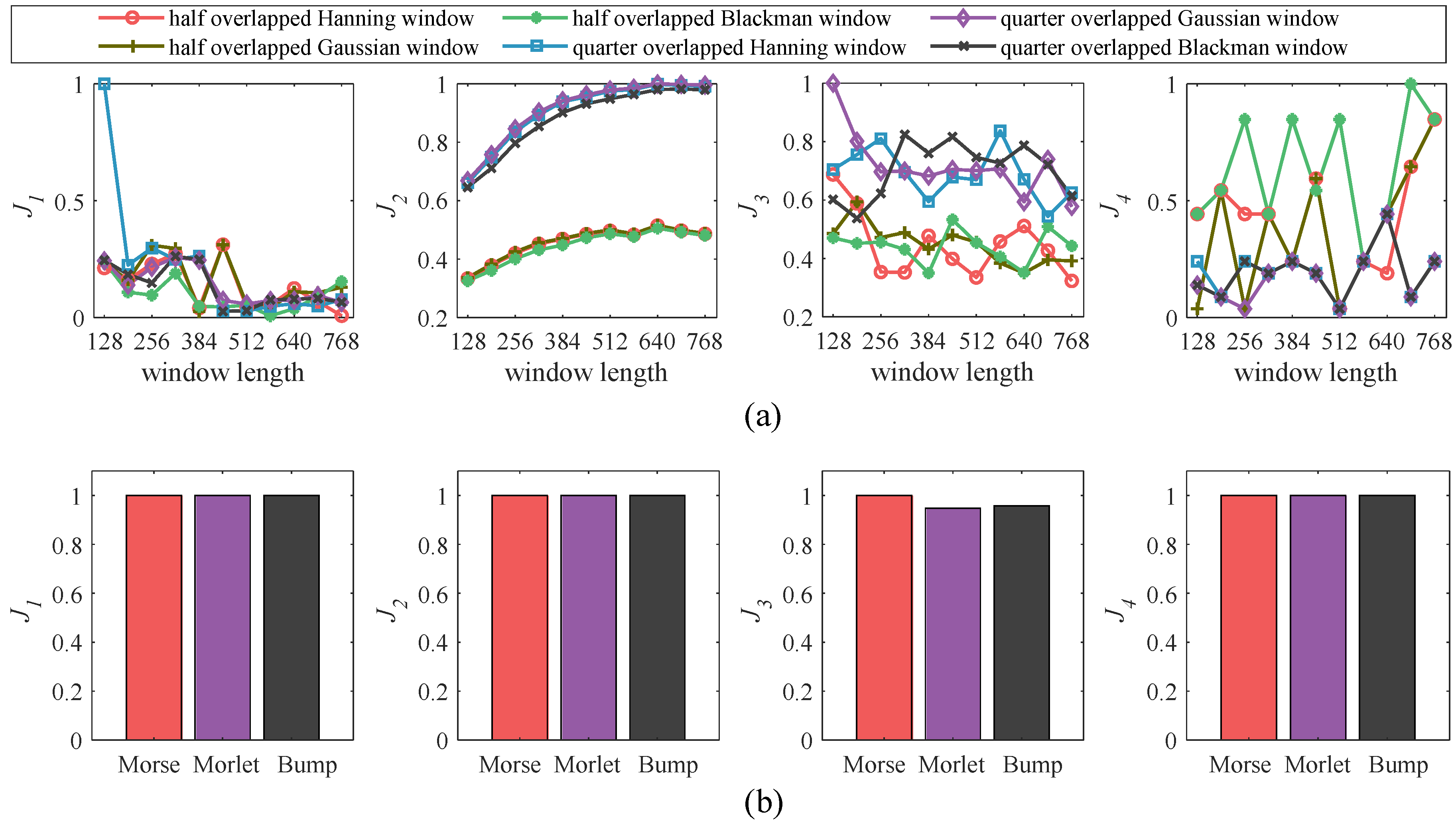
A parametric study was first conducted to study the influence of TFR parameters and select the optimal parameters in comparing performance across TFRs. The study starts with the STFT, where the window length and type are investigated. In the investigation, the window size ranged from 128 to 768 at an interval size of 64, window length overlaps were a half and a quarter of the window length, and windowing functions were Hanning, Gaussian, and Blackman, as shown in Figure 3. Figure 4a plots the results. To facilitate the comparison, the four metrics were normalized to the highest value at 1. It can be observed that both and converge after a window length of 512. In addition, under the and metrics, the half overlapped window performs better than the quarter overlapped windows. Under , the half overlapped Gaussian window performs similarly to the quarter overlapped windows. However, the other half overlapped window functions generally perform worse, and the window length of 512 appears to yield optimal results. From these results, a window length of 512 with a half-overlapping Gaussian windowing function was selected as the optimal set of parameters.
The parametric study for the WT consisted of evaluating the performance under different wavelets, including the Morse, Morlet, and Bump wavelets [30,31]. Figure 4a plots the results. Results show a similar performance across all wavelet types, with slightly better performance for the Morlet wavelet observable under . The Morlet wavelet was selected as the optimal parameter For the MSST, the number of 2 to 5 iterations were studied. Results were also similar across all iteration numbers, and thus a total of two iterations were selected as the optimal parameter.
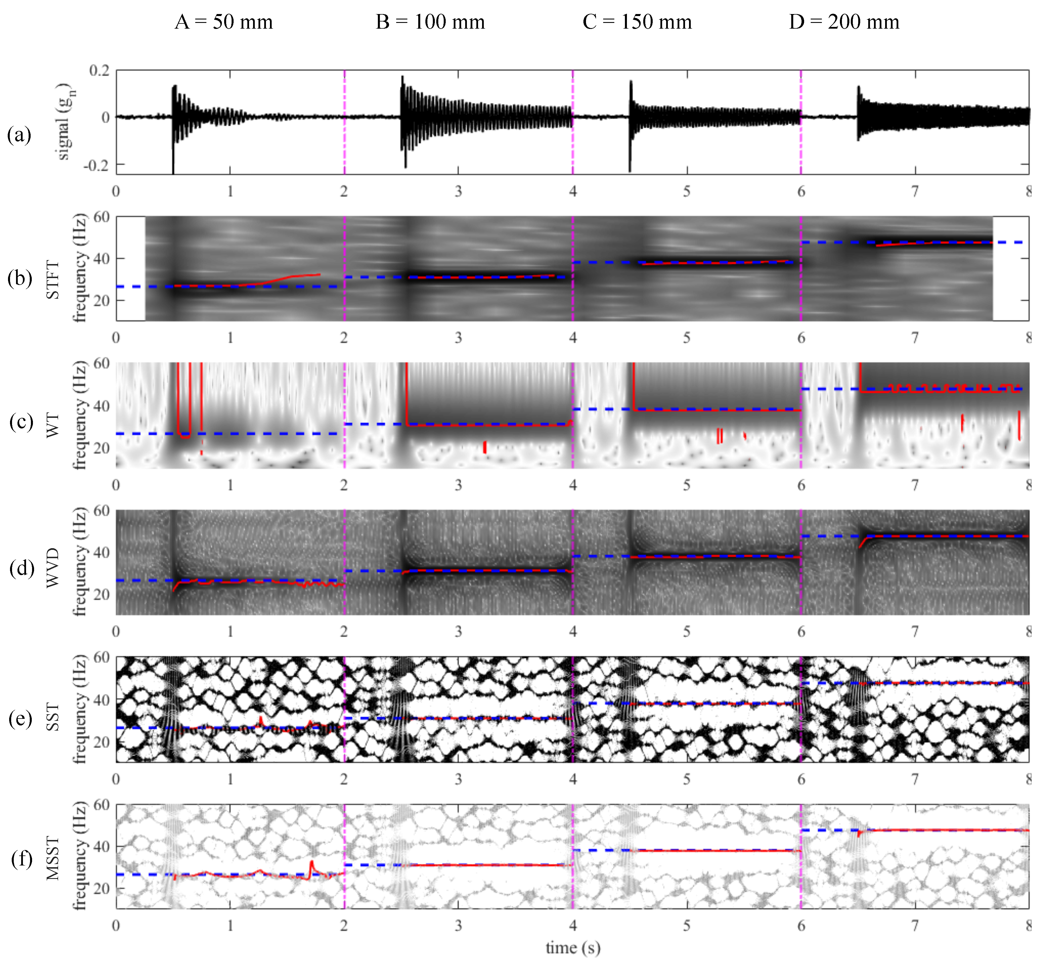
Results from the fixed cart configuration experiment using the selected optimal parameters are shown in Figure 5. Figure 5a is the time series response over 2 s under each location. Figure 5b–f show the time-frequency content extracted by the STFT, WT, WVD, SST, and MSST methods, respectively. Ridge detection is used to identify the first natural frequency (shown as a solid red line) by extracting the maximum-energy time-frequency ridge of the spectrograms [32]. The measured frequencies from the FRF (Figure 2c) are also shown in blue dashed lines. Table 1 lists performance under metrics –.
Visual observation of the time-frequency plane (Figure 5b–f) shows that the WVD provides the best frequency identification at position A, followed by the SST, while the WT yielded high variance in results. This may be attributed to the weaker acceleration response from the beam compared to other positions (Figure 5a). Over other positions, all methods appear to have identified a stable frequency, with the SST and MSST converging faster than the other methods, followed by the STFT. An examination of the performance metrics listed in Table 1 confirms these observations. The SST provided the most precise estimate of frequency, while the WT was the least precise (). The SST and MSST methods showed the highest energy concentrations (), as expected from time-frequency reassignment methods. However, their computation time () was significantly higher compared to the other methods, with the STFT and WT being the fastest. In terms of convergence (), the SST and MSST were the fastest, while the STFT was the slowest. From the static cart experiment results, it appears that the WT is one of the most applicable methods to the high-rate problem given its fast convergence speed and lower computation time, although at the cost of precision on the estimation of frequency over weak signals.
4.2. Moving Cart Configuration
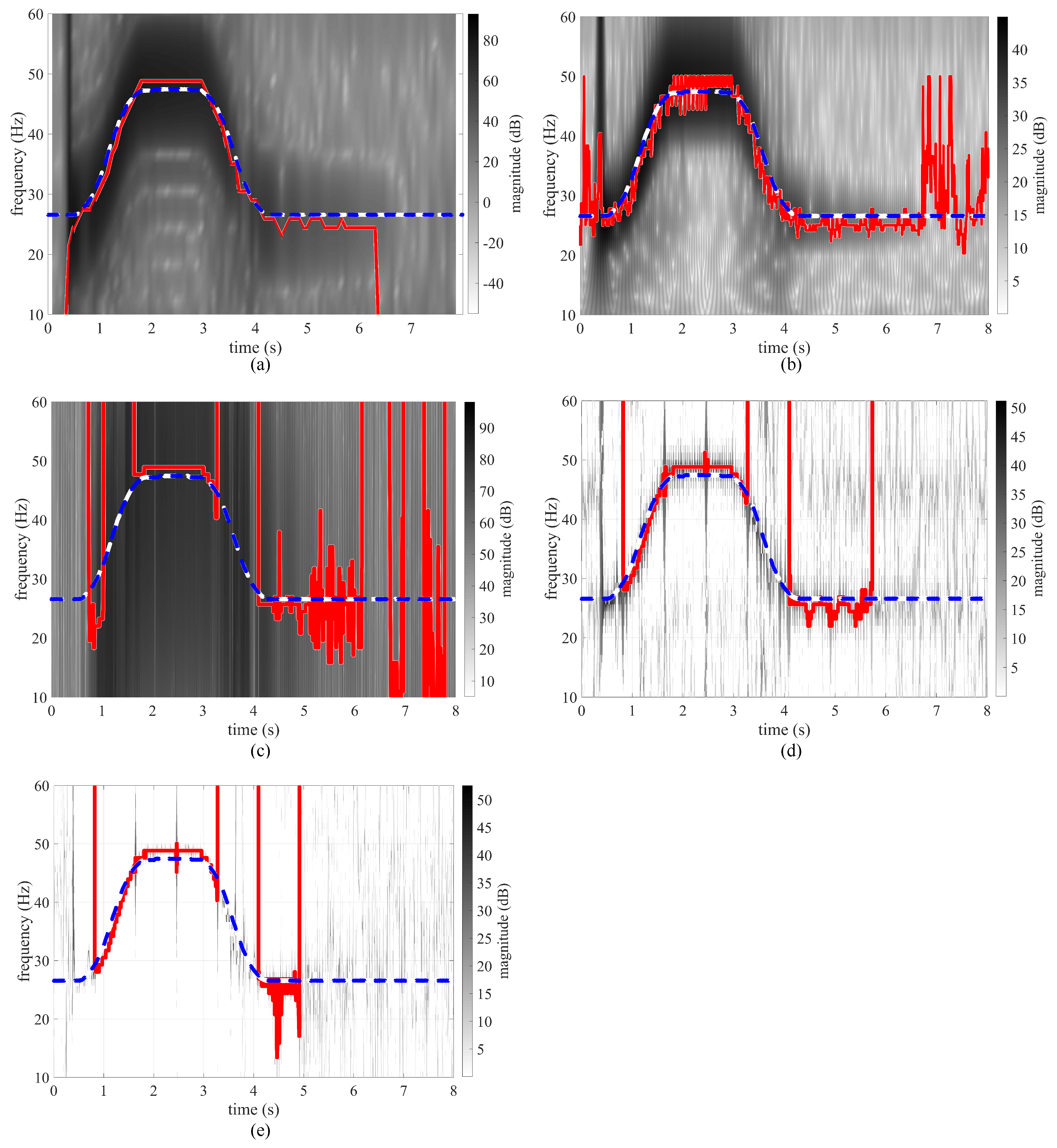
Time-frequency planes obtained from the moving cart experiment are shown in Figure 6. Results also show the estimated true temporal variation of the beam’s fundamental frequency (in dashed blue), obtained by assuming linearity of the system and interpolating between the measured frequencies from the FRF (Figure 2c) at the 50 mm and 200 mm positions. The STFT and WT were conducted with a sliding window of length 4096, corresponding to 164 ms, and the overlap size is half of the window length. Data were down-sampled from 25 kHz to 1.25 kHz to conduct the WVD in order to reduce the computational burden by maintaining a low-size window of 512 data points and improve the frequency resolution to bin sizes of 2.4 Hz, instead of 12.2 Hz under 25 kHz. The SST and MSST were processed with a non-overlapping sliding window size of 1024 data points at a reduced sampling rate of 1.25 kHz, corresponding to a duration of 819 ms. The WT was conducted using Morse wavelets, the SST used a Gaussian window, and the MSST was iterated five times, as for the fixed cart configuration. Table 2 lists results for performance metrics and , along with a summary of the processing window lengths used in the study.
A visual comparison of the fundamental frequency extracted by the TFR methods (solid red line) with the estimated true frequency (dashed blue line) in Figure 6 shows that the SFTF provided the most precise estimation of the beam’s fundamental frequency that can be linked to the cart’s location, followed by the WT. The WT showed more chattering in the results, but with a better adaptation to the varying frequency. This is confirmed by performance metric (Table 2), which also shows that the SST underperformed with respect to the other TFR methods. The computation time per iteration () was significantly faster for the STFT and WT methods, smaller than the window hopping time (82 ms). For the WVD, the down-sampling strategy enabled a computation time of 262 ms per window, instead of approximately 10 s using a window size of 2048 data points. However, despite such improvement in the frequency resolution and computational time, the WVD failed at identifying the beam frequency during the movement of the cart, as observable in Figure 6. The MSST’s computation time is significantly longer than for the other methods, attributable to the longer window lengths that were necessary in implementing the methods.
Results from the moving cart experiment showed that both the STFT and WT were adequate methods through their fast computational speed and acceptable precision on the frequency estimation. The three other methods did not provide adequate performance in terms of computation time. Moreover, the WVD did not succeed at extracting the fundamental frequency with acceptable precision. Overall, compared with results obtained under the fixed cart configuration experiment, it can be concluded that both the STFT and WT methods have good promise for real-time application to high-rate state estimation due to their fast computation time and level of precision. It is worth remarking that the WT’s precision relative to the STFT is approximately the same, unlike results seen under the fixed cart configuration where the WT’s estimation error was close to three times that of the STFT. This can be attributed to the faster convergence speed of the WT, whereas the WT was capable of adapting more quickly to a change in the system’s frequency under the moving cart configuration. Thus, it appears that the WT is more applicable to the high-rate problem, given its faster convergence speed, but this may come at the cost of lower precision on the estimation depending on circumstances.
5. Conclusions
This paper examined the promise of various time-frequency representation methods at conducting real-time high-rate state estimation. In particular, five methods were compared: the short-term Fourier transform (STFT), wavelet transform (WT), Wigner–Ville distribution (WVD), synchrosqueezing transform (SST), and multi-SST (MSST). The performance of the methods was assessed using high-rate experimental data produced on the DROPBEAR (Dynamic Reproduction of Projectiles in Ballistic Environments for Advanced Research) testbed. Such data included acceleration measurements of a beam with a cart located at fixed positions (“fixed cart configuration”) sampled at 1 kHz, and with a cart moving between two locations (“moving cart configuration”), sampled at 25 kHz.
Results from the fixed cart configuration show that both the STFT and WT methods could be performed significantly faster than the three other methods, with the WT outperforming other methods in terms of convergence speed. Under the moving cart experiment, both the STFT performed similarly in terms of frequency estimation precision, but with the STFT being computationally faster to implement. The WVD failed at identifying the fundamental frequency, while the SST and MSST had unacceptable computation times, attributable to the longer window lengths that were necessary for implementing the methods. The SST and MSST can achieve good energy concentration and estimation in fixed cart configuration, but not for the moving-cart configuration.
Overall, it appears that the WT would be a better candidate for real-time applicability to high-rate state-estimation given its relatively faster convergence, but this may come at the cost of lower precision on the estimation depending on circumstances. The performance of the WT is yet to be assessed for strongly time-varying systems to characterize high-rate mechanisms undergoing sudden and high amplitude changes in their dynamics. It should also be noted that this paper limited the investigation to only five methods over a very specific experimental dataset and that, while results point towards the WT method as a possible path to high-rate applications, different conclusions could be drawn in a different environment, in particular for systems dominated by higher frequencies. In general, it is envisioned that applications to the high-rate problem would come in the form of advanced yet computationally fast algorithms inspired by the STFT or WT methods and that their implementations in field-programmable gate arrays (FPGAs) would significantly improve their performance in terms of computation time.
Author Contributions
The authors made the following contributions: Conceptualization: J.Y., S.L., and A.S.; methodology: J.Y. and S.L.; software: J.Y.; resources: J.D.; writing—original draft preparation: J.Y. and P.S.; writing—review and editing: S.L. and A.S.; visualization: J.Y.; supervision: A.S. and S.L. All authors have read and agreed to the published version of the manuscript.
Funding
The work presented in this paper is partially funded by the National Science Foundation under award number CCSS-1937460. Their support is gratefully acknowledged. Any opinions, findings, and conclusions or recommendations expressed in this material are those of the authors and do not necessarily reflect the views of the sponsors.
Conflicts of Interest
The author(s) declared no potential conflicts of interest with respect to the research, authorship, and/or publication of this article.
Abbreviations
The following abbreviations are used in this manuscript:
| TFR | Time-frequency representation |
| STFT | Short-time Fourier Transform |
| WT | Wavelet transform |
| WVD | Wigner–Ville distribution |
| SST | Synchrosqueezed transform |
| MSST | Multi-synchrosqueezed transform |
References
- Hong, J.; Laflamme, S.; Dodson, J.; Joyce, B. Introduction to State Estimation of High-Rate System Dynamics. Sensors 2018, 18, 217. [Google Scholar] [CrossRef] [Green Version]
- Dodson, J.; Joyce, B.; Hong, J.; Laflamme, S.; Wolfson, J. Microsecond State Monitoring of Nonlinear Time-Varying Dynamic Systems. Volume 2: Modeling, Simulation and Control of Adaptive Systems Integrated System Design and Implementation Structural Health Monitoring. Proceedings of the ASME 2017 Conference on Smart Materials, Adaptive Structures and Intelligent Systems, Snowbird, UT, USA, 18–20 September 2017, American Society of Mechanical Engineers: New York, NY, USA, 2017. [Google Scholar] [CrossRef] [Green Version]
- Hong, J.; Laflamme, S.; Cao, L.; Dodson, J.; Joyce, B. Variable input observer for nonstationary high-rate dynamic systems. Neural Comput. Appl. 2018, 32, 5015–5026. [Google Scholar] [CrossRef] [Green Version]
- Kumar, R.; Syam, P.; Das, S.; Chattopadhyay, A.K. Review on model reference adaptive system for sensorless vector control of induction motor drives. IET Electr. Power Appl. 2015, 9, 496–511. [Google Scholar] [CrossRef]
- Yan, J.; Laflamme, S.; Leifsson, L. Computational Framework for Dense Sensor Network Evaluation Based on Model-Assisted Probability of Detection. Mater. Eval. 2020, 78. [Google Scholar] [CrossRef]
- Yan, J.; Laflamme, S.; Hong, J.; Dodson, J. Online Parameter Estimation under Non-Persistent Excitations for High-Rate Dynamic Systems. In Review.
- Downey, A.; Hong, J.; Dodson, J.; Carroll, M.; Scheppegrell, J. Millisecond model updating for structures experiencing unmodeled high-rate dynamic events. Mech. Syst. Signal Process. 2020, 138, 106551. [Google Scholar] [CrossRef]
- Boashash, B. Chapter 15—Time-Frequency Diagnosis, Condition Monitoring, and Fault Detection. In Time-Frequency Signal Analysis and Processing, 2nd ed.; Boashash, B., Ed.; Academic Press: Oxford, UK, 2016; pp. 857–913. [Google Scholar] [CrossRef]
- Goyal, D.; Pabla, B.S. The Vibration Monitoring Methods and Signal Processing Techniques for Structural Health Monitoring: A Review. Arch. Comput. Methods Eng. 2015, 23, 585–594. [Google Scholar] [CrossRef]
- Dörfler, M.; Matusiak, E. Nonstationary Gabor frames-approximately dual frames and reconstruction errors. Adv. Comput. Math. 2015, 41, 293–316. [Google Scholar] [CrossRef] [Green Version]
- Paul Busch, T.H.; Lahti, P. Heisenberg’s uncertainty principle. Phys. Rep. 2007, 452, 155–176. [Google Scholar] [CrossRef] [Green Version]
- Huang, N.E.; Shen, Z.; Long, S.R.; Wu, M.C.; Shih, H.H.; Zheng, Q.; Yen, N.C.; Tung, C.C.; Liu, H.H. The empirical mode decomposition and the Hilbert spectrum for nonlinear and non-stationary time series analysis. Proc. R. Soc. Lond. Ser. Math. Phys. Eng. Sci. 1998, 454, 903–995. [Google Scholar] [CrossRef]
- Chen, Y.; Liu, T.; Chen, X.; Li, J.; Wang, E. Time-frequency analysis of seismic data using synchrosqueezing wavelet transform. IEEE Geosci. Remote. Sens. Lett. 2014, 11, 2042–2044. [Google Scholar] [CrossRef] [Green Version]
- Yuan, M.; Sadhu, A.; Liu, K. Condition assessment of structure with tuned mass damper using empirical wavelet transform. J. Vib. Control 2017, 24, 4850–4867. [Google Scholar] [CrossRef]
- Sadhu, A.; Sony, S.; Friesen, P. Evaluation of progressive damage in structures using tensor decomposition-based wavelet analysis. J. Vib. Control 2019, 25, 2595–2610. [Google Scholar] [CrossRef]
- Mahato, S.; Chakraborty, A. Sequential clustering of synchrosqueezed wavelet transform coefficients for efficient modal identification. J. Civ. Struct. Health Monit. 2019, 9, 271–291. [Google Scholar] [CrossRef]
- Yu, G.; Wang, Z.; Zhao, P. Multisynchrosqueezing Transform. IEEE Trans. Ind. Electron. 2019, 66, 5441–5455. [Google Scholar] [CrossRef]
- Soudan, M.; Vogel, C. Correction Structures for Linear Weakly Time-Varying Systems. IEEE Trans. Circuits Syst. Regul. Pap. 2012, 59, 2075–2084. [Google Scholar] [CrossRef]
- Pham, D.H.; Meignen, S. High-Order Synchrosqueezing Transform for Multicomponent Signals Analysis—With an Application to Gravitational-Wave Signal. IEEE Trans. Signal Process. 2017, 65, 3168–3178. [Google Scholar] [CrossRef] [Green Version]
- Joyce, B.; Dodson, J.; Laflamme, S.; Hong, J. An Experimental Test Bed for Developing High-Rate Structural Health Monitoring Methods. Shock Vib. 2018, 2018, 1–10. [Google Scholar] [CrossRef]
- Gabor, D. Theory of communication. Part 1: The analysis of information. J. Inst. Electr.-Eng.-Part III Radio Commun. Eng. 1946, 93, 429–441. [Google Scholar] [CrossRef] [Green Version]
- Feng, Z.; Liang, M.; Chu, F. Recent advances in time–frequency analysis methods for machinery fault diagnosis: A review with application examples. Mech. Syst. Signal Process. 2013, 38, 165–205. [Google Scholar] [CrossRef]
- Mallat, S. A wavelet tour of signal processing. In The Sparse Way; Elsevier: Amsterdam, The Netherlands, 1999. [Google Scholar]
- Flandrin, P. Time-Frequency/Time-Scale Analysis; Academic press: Cambridge, MA, USA, 1998. [Google Scholar]
- Boashash, B.; Black, P. An efficient real-time implementation of the Wigner–Ville distribution. IEEE Trans. Acoust. Speech Signal Process. 1987, 35, 1611–1618. [Google Scholar] [CrossRef]
- Bradford, S.C. Time-Frequency Analysis of Systems with Changing Dynamic Properties; Earthquake Engineering Research Laboratory: Reno, NV, USA, 2006. [Google Scholar]
- Thakur, G. The Synchrosqueezing transform for instantaneous spectral analysis. In Excursions in Harmonic Analysis; Springer: Berlin/Heidelberg, Germany, 2015; Volume 4, pp. 397–406. [Google Scholar] [CrossRef] [Green Version]
- Ewins, D.J. Modal Testing: Theory, Practice, and Application; Research Studies Press: Letchworth, UK; Philadelphia, PA, USA, 2000. [Google Scholar]
- Chen, G.; Chen, J.; Dong, G. Chirplet Wigner–Ville distribution for time–frequency representation and its application. Mech. Syst. Signal Process. 2013, 41, 1–13. [Google Scholar] [CrossRef]
- Olhede, S.; Walden, A. Generalized Morse wavelets. IEEE Trans. Signal Process. 2002, 50, 2661–2670. [Google Scholar] [CrossRef] [Green Version]
- Li, L.; Cai, H.; Jiang, Q. Adaptive synchrosqueezing transform with a time-varying parameter for non-stationary signal separation. Appl. Comput. Harmon. Anal. 2020, 49. [Google Scholar] [CrossRef] [Green Version]
- Iatsenko, D.; McClintock, P.; Stefanovska, A. Extraction of instantaneous frequencies from ridges in time–frequency representations of signals. Signal Process. 2016, 125, 290–303. [Google Scholar] [CrossRef] [Green Version]
Figure 1.
DROPBEAR testbed: (a) picture and (b) schematic of the setup.

Figure 2.
(a) signal from the fixed cart configuration at 50, 100, 150, and 200 mm; (b) signal from moving cart configuration between 50 mm to 200 mm; and (c) frequency response functions (FRFs) for DROPBEAR with fixed cart positions at 50, 100, 150, and 200 mm.
Figure 2.
(a) signal from the fixed cart configuration at 50, 100, 150, and 200 mm; (b) signal from moving cart configuration between 50 mm to 200 mm; and (c) frequency response functions (FRFs) for DROPBEAR with fixed cart positions at 50, 100, 150, and 200 mm.

Figure 3.
Window functions used in STFT.

Figure 4.
Parametric investigation for (a) STFT; and (b) WT.

Figure 5.
Time-frequency planes from the fixed cart configuration obtained using the (a) signal from the fixed cart configuration at 50, 100, 150, and 200 mm; (b) STFT; (c) WT; (d) WVD; (e) SST; and (f) MSST method with extracted frequencies (red solid lines) and estimated true frequencies (dashed blue lines).

Figure 6.
Time-frequency planes from the fixed cart configuration obtained using the (a) STFT; (b) WT; (c) WVD; (d) SST; and (e) MSST method with extracted frequencies (red solid lines) and estimated true frequencies (dashed blue lines).
Figure 6.
Time-frequency planes from the fixed cart configuration obtained using the (a) STFT; (b) WT; (c) WVD; (d) SST; and (e) MSST method with extracted frequencies (red solid lines) and estimated true frequencies (dashed blue lines).


Table 1.
Fixed cart configuration time-frequency analysis comparison.
| TFR | ||||
|---|---|---|---|---|
| Method | (Hz) | () | (ms) | (ms) |
| STFT | 0.384 | 0.012 | 6.9 | 286 |
| WT | 0.729 | 0.0220 | 242 | 44 |
| WVD | 0.316 | 0.0573 | 1093 | 51 |
| SST | 0.095 | 1 | 10,505 | 1 |
| MSST | 0.155 | 0.6667 | 12,236 | 1 |
Table 2.
Moving cart configuration time-frequency analysis comparison.
| TFR | Window | ||
|---|---|---|---|
| Method | (Hz) | (ms) | (ms) |
| STFT | 0.54 | 3.8 | 82 |
| WT | 0.56 | 9.3 | 82 |
| WVD | 1.88 | 262 | 819 |
| SST | 0.91 | 288 | 819 |
| MSST | 0.66 | 543 | 819 |
© 2020 by the authors. Licensee MDPI, Basel, Switzerland. This article is an open access article distributed under the terms and conditions of the Creative Commons Attribution (CC BY) license (http://creativecommons.org/licenses/by/4.0/).
Share and Cite
MDPI and ACS Style
Yan, J.; Laflamme, S.; Singh, P.; Sadhu, A.; Dodson, J. A Comparison of Time-Frequency Methods for Real-Time Application to High-Rate Dynamic Systems. Vibration 2020, 3, 204-216. https://0-doi-org.brum.beds.ac.uk/10.3390/vibration3030016
AMA Style
Yan J, Laflamme S, Singh P, Sadhu A, Dodson J. A Comparison of Time-Frequency Methods for Real-Time Application to High-Rate Dynamic Systems. Vibration. 2020; 3(3):204-216. https://0-doi-org.brum.beds.ac.uk/10.3390/vibration3030016
Chicago/Turabian StyleYan, Jin, Simon Laflamme, Premjeet Singh, Ayan Sadhu, and Jacob Dodson. 2020. "A Comparison of Time-Frequency Methods for Real-Time Application to High-Rate Dynamic Systems" Vibration 3, no. 3: 204-216. https://0-doi-org.brum.beds.ac.uk/10.3390/vibration3030016