An Inverse Problem for Quantum Trees with Delta-Prime Vertex Conditions

Abstract

In this paper, we consider a non-standard dynamical inverse problem for the wave equation on a metric tree graph. We assume that the so-called delta-prime matching conditions are satisfied at the internal vertices of the graph. Another specific feature of our investigation is that we use only one boundary actuator and one boundary sensor, all other observations being internal. Using the Neumann-to-Dirichlet map (acting from one boundary vertex to one boundary and all internal vertices) we recover the topology and geometry of the graph together with the coefficients of the equations.

1. Introduction

This paper concerns inverse problems for differential equations on quantum graphs. Under quantum graphs or differential equation networks (DENs) we understand differential operators on geometric graphs coupled by certain vertex matching conditions. Network-like structures play a fundamental role in many problems of science and engineering. The range for the applications of DENs is enormous. Here is a list of a few.

–Structural Health Monitoring. DENs, classically, arise in the study of stability, health, and oscillations of flexible structures that are made of strings, beams, cables, and struts. Analysis of these networks involve DENs associated with heat, wave, or beam equations whose parameters inform the state of the structure, see, e.g., [1].

–Water, Electricity, Gas, and Traffic Networks. An important example of DENs is the Saint-Venant system of equations, which model hydraulic networks for water supply and irrigation, see, e.g., [2]. Other important examples of DENs include the telegrapher equation for modeling electric networks, see, e.g., [3], the isothermal Euler equations for describing the gas flow through pipelines, see, e.g., [4], and the Aw-Rascle equations for describing road traffic dynamics, see e.g., [5].

–Nanoelectronics and Quantum Computing. Mesoscopic quasi-one-dimensional structures such as quantum, atomic, and molecular wires are the subject of extensive experimental and theoretical studies, see, e.g., [6], the collection of papers in [7,8,9]. The simplest model describing conduction in quantum wires is the Schrödinger operator on a planar graph. For similar models appear in nanoelectronics, high-temperature superconductors, quantum computing, and studies of quantum chaos, see, e.g., [10,11,12].

–Material Science. DENs arise in analyzing hierarchical materials like ceramic and metallic foams, percolation networks, carbon and graphene nano-tubes, and graphene ribbons, see, e.g., [13,14,15].

–Biology. Challenging problems involving ordinary and partial differential equations on graphs arise in signal propagation in dendritic trees, particle dispersal in respiratory systems, species persistence, and biochemical diffusion in delta river systems, see, e.g., [16,17,18].

Quantum graph theory gives rise to numerous challenging problems related to many areas of mathematics from combinatoric graph theory to PDE and spectral theories. A number of surveys and collections of papers on quantum graphs appeared in previous years; we refer to the monograph by Berkolaiko and Kuchment, [19], for a complete reference list. The inverse theory of network-like structures is an important part of a rapidly developing area of applied mathematics—analysis on graphs. It is tremendously important for all aforementioned applications. In this paper, we solve a non-standard dynamical inverse problem for the wave equation on a metric tree graph.

Let $\mathsf{\Omega }=\{V,E\}$ be a finite compact and connected metric tree (i.e., graph without cycles), where V is a set of vertices and E is a set of edges. We recall that a graph is called a metric graph if every edge $e_j\in E,j=1,\dots ,N,$ is identified with an interval $(a_{2j-1},a_{2j})$ of the real line with a positive length $l_j.$ We denote the boundary vertices (i.e., vertices of degree one) by $\mathsf{\Gamma }=\{{\gamma }_0,\dots ,{\gamma }_m\}$, and interior vertices (whose degree is at least 2) by $\{v_{m+1},\dots ,v_N\}$. The vertices can be regarded as equivalence classes of the edge end points $a_j$. For each vertex $v_k$, denote its degree by ${\mathsf{{\rm Y}}}_k$. We write $j\in J\left(v\right)$ if $e_j\in E\left(v\right),$ where $E\left(v\right)$ is the set of edges incident to $v.$

The graph $\mathsf{\Omega }$ determines naturally the Hilbert space of square integrable functions $\mathcal{H}=L^2\left(\mathsf{\Omega }\right).$ We define its subspace ${\mathcal{H}}^1$ as the space of functions y on $\mathsf{\Omega }$ such that ${y|}_e\in H^1\left(e\right)$ for every $e\in E$ and ${y|}_{\mathsf{\Gamma }\backslash \left\{{\gamma }_0\right\}}=0,$ and let ${\mathcal{H}}^{-1}$ be the dual space to ${\mathcal{H}}^1$. When convenient, we denote the restriction of a function w on $\mathsf{\Omega }$ to $e_j$ by $w_j$. For any vertex $v_k$ and function $w\left(x\right)$ on the graph, we denote by $\partial w_j\left(v_k\right)$ the derivative of $w_j$ at $v_k$ in the direction pointing away from the vertex.

Our system is described by the following initial boundary value problem (IBVP) with so-called delta-prime compatibility conditions at each internal vertex $v_k$:

$$\begin{array}{ccc}\hfill u_{tt}-u_{xx}+qu& =& 0,(x,t)\in (\mathsf{\Omega }\backslash V)\times [0,T],\hfill \end{array}$$

(1)

$$\begin{array}{ccc}\hfill {u|}_{t=0}=u_t{|}_{t=0}& =& 0,x\in \mathsf{\Omega },\hfill \end{array}$$

(2)

$$\begin{array}{ccc}\hfill \partial u_i(v_k,t)& =& \partial u_j(v_k,t),i,j\in J\left(v_k\right),v_k\in V\backslash \mathsf{\Gamma },t\in [0,T],\hfill \end{array}$$

(3)

$$\begin{array}{ccc}\hfill \sum _{j\in J\left(v_k\right)}{u}_j(v_k,t)& =& 0,v_k\in V\backslash \mathsf{\Gamma },t\in [0,T],\hfill \end{array}$$

(4)

$$\begin{array}{ccc}\hfill \frac{\partial u}{\partial x}({\gamma }_0,t)& =& f\left(t\right),t\in [0,T],\hfill \end{array}$$

(5)

$$\begin{array}{ccc}\hfill u({\gamma }_k,t)& =& 0,k=1,\dots ,m,t\in [0,T].\hfill \end{array}$$

(6)

Here, T is arbitrary positive number, $q_j\in C\left([a_{2j-1},a_{2j}]\right)$ for all j, and $f\in L^2(0,T)$. The physical interpretation of conditions (3) and (4), and some other matching conditions was discussed in [20].

The well-posedness of this system is discussed in Section 2; it will be proved that $u\in C([0,T];{\mathcal{H}}^1)\cap C^1([0,T];\mathcal{H}).$ In what follows, we refer to ${\gamma }_0$ as the root of $\mathsf{\Omega }$ and f as the control.

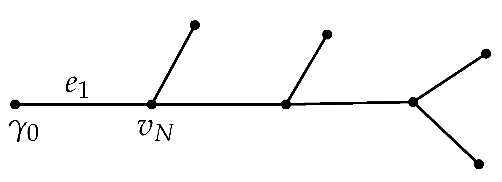
We now pose our inverse problem. Assume an observer knows the boundary condition (5), and that (6) holds at the other boundary vertices, and that the graph is a tree. The unknowns are the number of boundary vertices and interior vertices, the adjacency relations for this tree, i.e., for each pair of vertices, whether or not there is an edge joining them, the lengths $\left\{{\ell }_j\right\}$, and the function q. We wish to determine these quantities with a set of measurements that we describe now. We can suppose $v_N$ is the interior vertex adjacent to ${\gamma }_0$ with $e_1$ the edge joining the two, see Figure 1. Our first measurement is then the following measurement at ${\gamma }_0$:

$$\left(R_{0,1}f\right)\left(t\right):=u_1^f({\gamma }_0,t).$$

(7)

We show that from operator $R_{0,1}$ one can recover ${\ell }_1$ and the degree ${\mathsf{{\rm Y}}}_N$ of $v_N$. Then by a well known argument, see [21], one can then determine $q_1$.

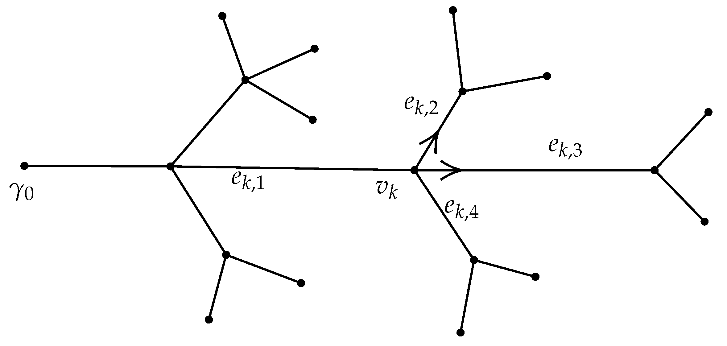
Having established these quantities, in our second step, we propose to place sensors on the edges incident to $v_N$, and using these measurements together with $R_{0,1}$ to determine the data associated to these edges. Note that the one control remains at ${\gamma }_0$. The goal is to repeat these steps until all data associated to the graph have been determined. To define the interior measurements we require more notation. For each interior vertex $v_k$ we list the incident edges by $\{e_{k,j}:j=1,\dots ,{\mathsf{{\rm Y}}}_k\}$. Here $e_{k,1}$ is chosen to be the edge lying on the unique path from ${\gamma }_0$ to $v_k$, and the remaining edges are labeled randomly, see Figure 2. Then the sensors measure

$$\left(R_{k,j}f\right)\left(t\right):=u_j^f(v_k,t),k=m+1,\dots ,N,j=2,\dots ,{\mathsf{{\rm Y}}}_k-1.$$

(8)

We show that we do not need sensors at $e_{k,1},e_{k,{\mathsf{{\rm Y}}}_k}$. Thus the total number of sensors is $1+{\sum }_{j=m+1}^N({\mathsf{{\rm Y}}}_j-2)$. It is easy to check that this number is equal to $\left|\mathsf{\Gamma }\right|-1.$ We denote by $R^T$ the $\left(\right|\mathsf{\Gamma }|-1)$-tuple $(R_{0,1},R_{N,2},R_{N,3},\dots )$ acting on $L^2(0,T).$

2. Results

Let ℓ be equal to the maximum distance between ${\gamma }_0$ and any other boundary vertex. Our main result is the following

Theorem 1.

Assume $q_j\in C\left([a_{2j-1},a_{2j}]\right)$ for all $j.$ Suppose $T<2\ell$. Then from $R^T$ one can determine the number of interior and boundary vertices, the adjacency relations of the tree, q, and the lengths of the edges.

3. Discussion

We now compare this result to others in the literature. We are unaware of any works treating the inverse problem on general tree graphs with delta-prime conditions on the internal vertices. The most common conditions for internal vertices are continuity together with Kirchhoff–Neumann condition: ${\sum }_{j\in J\left(v_k\right)}\partial u_j(v_k,t)=0$ and all references in this paragraph assume these conditions. In [21], the authors assume that controls and measurements take place at all boundary vertices but one. The authors use an iterative method called “leaf peeling”, where the response operator on $\mathsf{\Omega }$ is used first to determine the data on the edges adjacent to the boundary, and then to determine the response operator associated to a proper subgraph. In [21], the leaf peeling argument includes spectral methods that require knowing $R^T$ for all T. In [22], the methods of [21] are extended to the case where masses are placed at internal vertices, see also [23]; however these methods still require knowledge of $R^T$ for all T. Also in [22], it is proven that that for a single string of length ℓ with N attached masses and $T<2\ell$, $R_{0,1}^T$ is sufficient to solve the inverse problem. In particular, [23] uses a spectral variant of the boundary control method, together with the relationship between the response operator and the connecting operator. In [24,25], a dynamical leaf peeling argument is developed for a tree with no masses and with response operators at all but one boundary points, allowing for the solution of the inverse problem for finite T sufficiently large. An important ingredient in their leaf peeling is determining the response operators associated with subtrees, called “reduced response operators”, from the response operator associated to the original tree. In all of these papers, it is assumed that there are no interior measurements. In [26], the iterative methods from [24,25,27] are adapted to a tree with masses placed at internal vertices, with a single control at the roof and measurements there and at internal vertices. For other works on quantum graphs, see [1,16,19,28,29,30,31].

A special feature of the present paper is that we use only one control together internal observations. This may be useful in some physical settings where some or most boundary points are inaccessible. Another potential advantage of the method presented here is that we recover all parameters of the graphs, including its topology, from the $\left(\right|\mathsf{\Gamma }|-1)$-tuple response operator acting on $L^2(0,T).$ In previous papers, the authors recovered the graph topology from a larger number of measurements: the $\left(\right|\mathsf{\Gamma }|-1)\times \left(\right|\mathsf{\Gamma }|-1)$ matrix (boundary) response operator or, equivalently, from $\left(\right|\mathsf{\Gamma }|-1)\times \left(\right|\mathsf{\Gamma }|-1)$ Titchmarsh–Weyl matrix function. In [32], the inverse problems on a star graph for the wave equation with general self-adjoint matching conditions was solved by the $\left(\right|\mathsf{\Gamma }|-1)\times \left(\right|\mathsf{\Gamma }|-1)$ matrix boundary response operator.

4. Materials and Methods

4.1. Preliminaries

In what follows, we use the notations

$${\mathcal{F}}^n=\{f\in {\mathcal{H}}^n\left(\mathbb{R}\right):f\left(t\right)=0\mathrm{if}t\le 0\},$$

(9)

where ${\mathcal{H}}^n\left(\mathbb{R}\right)$ are the standard Sobolev spaces. We define the Heaviside function by $H\left(t\right)=1$ for $t<0$, and $H\left(t\right)=0$ for $t<0$. Then, we define $H_n\in {\mathcal{F}}^n$ as the unique solution to

$$\frac{d^n}{d{t}^n}{H}_n=H;$$

at times we use $H_{-1}\left(t\right),$ resp. $H_{-2}\left(t\right)$ for $\delta \left(t\right),$ resp. ${\delta }^{\prime }\left(t\right).$ Here $\delta \left(t\right)$ denotes the Dirac delta function supported at $t=0$. In this section and those that follow, we drop the superscript T from $R^T$ when convenient.

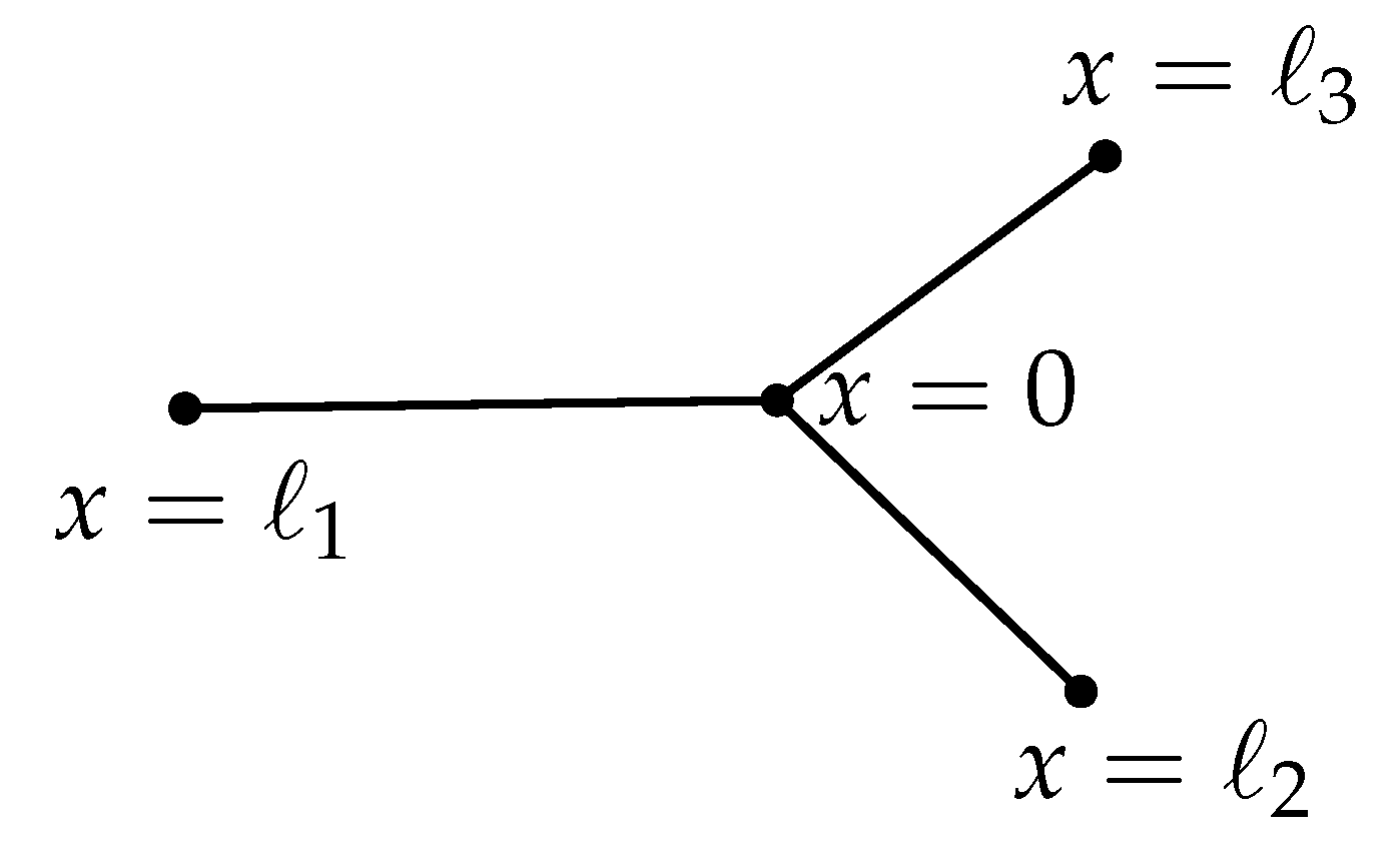
Consider a star shaped graph with edges $e_1,\dots ,e_N$. For each j, we identify $e_j$ with the interval $(0,{\ell }_j)$ and the central vertex with $x=0$, see Figure 3.

Recall the notation $q_j{=q|}_{e_j}$, and $u_j{(\ast ,t)=u(\ast ,t)|}_{e_j}$. Thus, we consider the system

$$\begin{array}{ccc}\hfill \frac{{\partial }^{2}u}{\partial t^2}-\frac{{\partial }^{2}u}{\partial x^2}+qu& =& 0,x\in e_j,j=1,\dots ,N,t\in \times [0,T],\hfill \end{array}$$

(10)

$$\begin{array}{ccc}\hfill {u|}_{t=0}=u_t{|}_{t=0}& =& 0,\hfill \end{array}$$

(11)

$$\begin{array}{ccc}\hfill \partial u_i(0,t)& =& \partial u_j(0,t),i\ne j,t\in [0,T],\hfill \end{array}$$

(12)

$$\begin{array}{ccc}\hfill \sum _{j=1}^N{u}_j(0,t)& =& 0,t\in [0,T],\hfill \end{array}$$

(13)

$$\begin{array}{ccc}\hfill \partial u_1({\ell }_1,t)& =& f\left(t\right),t\in [0,T],\hfill \end{array}$$

(14)

$$\begin{array}{ccc}\hfill u_j({\ell }_j,t)& =& 0,j=2,\dots ,N,t\in [0,T].\hfill \end{array}$$

(15)

Let $u^f$ solve (10)–(15), and set

$$g_j\left(t\right)=u_j^f(0,t),j=1,\dots ,N.$$

(16)

For (11), it is standard that the waves have unit speed of propagation on the interval, so $g_j\left(t\right)=0$ for $t<{\ell }_1$ and all j. It will be useful first to consider the vibrating string on an interval.

4.2. Representation of Solution on an Interval and Reduced Response Operator

We adapt a representation of $u^f(x,t)$ developed in [27], where only Dirichlet control and boundary conditions were considered. Fix $j\in \{1,\dots ,N\}$. We extend $q_j$ to $(0,\infty )$ as follows: first evenly with respect to $x={\ell }_j$, and then periodically. Thus $q_j(2k{\ell }_j\pm x)=q_j\left(x\right)$ for all positive integers k.

Define $w_j$ to be the solution to the Goursat-type problem

$$\left\{\begin{array}{cc}\frac{\partial w^2}{\partial s^2}(x,s)-\frac{\partial w^2}{\partial x^2}(x,s)+q_j\left(x\right)w(x,s)=0,& 0<x<s<\infty ,\\ w_x(0,s)=0,w(x,x)=-\frac{1}{2}{\int }_0^x{q}_j\left(\eta \right)d\eta ,x<0.\end{array}\right.$$

A proof of solvability of this problem can be found in [33].

Consider the IBVP on the interval $(0,{\ell }_j)$:

$$\begin{array}{ccc}\hfill {\tilde{u}}_{tt}-{\tilde{u}}_{xx}+q_j\left(x\right)\tilde{u}& =& 0,0<x<{\ell }_j,t\in (0,T),\hfill \end{array}$$

(17)

$$\begin{array}{ccc}\hfill \tilde{u}(x,0)={\tilde{u}}_t(x,0)& =& 0,0<x<{\ell }_j,\hfill \end{array}$$

(18)

$$\begin{array}{ccc}\hfill \partial \tilde{u}(0,t)& =& p\left(t\right),\hfill \end{array}$$

(19)

$$\begin{array}{ccc}\hfill \tilde{u}({\ell }_j,t)& =& 0,t>0.\hfill \end{array}$$

(20)

Let $P\left(t\right)=-{\int }_0^{t}p\left(s\right)ds.$ Then, the solution to (17)–(20) on $e_j$ can be written as

$${\tilde{u}}_j^p(x,t)=\sum _{n\ge 0:0\le 2n{\ell }_j+x\le t}{(-1)}^n\left(P(t-2n{\ell }_j-x)+{\int }_{2n{\ell }_j+x}^t{w}_j(2n{\ell }_j+x,s)P(t-s)ds\right)$$

$$+\sum _{n\ge 1:0\le 2n{\ell }_j-x\le t}{(-1)}^n\left(P(t-2n{\ell }_j+x)+{\int }_{2n{\ell }_j-x}^t{w}_j(2n{\ell }_j-x,s)P(t-s)ds\right).$$

(21)

In what follows, we only consider $t\le T$ for some finite T, so all sums will be finite.

Let us now change the condition (20) to ${\tilde{u}}_x({\ell }_j,t)=0$. In this case, the solution becomes

$$\begin{array}{ccc}\hfill {\tilde{u}}_j^p(x,t)& =& \sum _{n\ge 0:0\le 2n{\ell }_j+x\le t}\left(P(t-2n{\ell }_j-x)+{\int }_{2n{\ell }_j+x}^t{w}_j(2n{\ell }_j+x,s)P(t-s)ds\right)\hfill \\ & & +\sum _{n\ge 1:0\le 2n{\ell }_j-x\le t}\left(P(t-2n{\ell }_j+x)+{\int }_{2n{\ell }_j-x}^t{w}_j(2n{\ell }_j-x,s)P(t-s)ds\right).\hfill \end{array}$$

To represent the solution of the wave equation on the edge $e_1$ in a star graph, we must account for the control at $x={\ell }_1$. Thus it will also be useful to represent the solution of a wave equation on an interval when the control is on the right end. Consider the IBVP:

$$\begin{array}{ccc}\hfill v_{tt}-v_{xx}+q_1\left(x\right)v& =& 0,0<x<{\ell }_1,t>0,\hfill \\ \hfill v(x,0)=v_t(x,0)& =& 0,0<x<{\ell }_1,\hfill \\ \hfill \partial v(0,t)& =& 0,\hfill \\ \hfill \partial v({\ell }_1,t)& =& f\left(t\right),t>0.\hfill \end{array}$$

(22)

Set ${\tilde{q}}_1\left(x\right)=q_1({\ell }_1-x)$, and extend ${\tilde{q}}_1$ to $[0,\infty )$ by ${\tilde{q}}_1(2k{\ell }_1\pm x)={\tilde{q}}_1\left(x\right)$. Define $k_1$ to be the solution to the Goursat-type problem

$$\left\{\begin{array}{cc}\frac{\partial k^2}{\partial s^2}(x,s)-\frac{\partial k^2}{\partial x^2}(x,s)+{\tilde{q}}_1\left(x\right)k(x,s)=0,& 0<x<s,\\ k_x(0,s)=0,k(x,x)=-\frac{1}{2}{\int }_0^x{\tilde{q}}_1\left(\eta \right)d\eta ,x<{\ell }_j.\end{array}\right.$$

Let $F\left(t\right)=-{\int }_0^{t}f\left(s\right)ds$. One can then verify that

$$\begin{array}{ccc}\hfill v^f(x,t)& =& F(t-{\ell }_1+x)+{\int }_{{\ell }_1-x}^t{k}_1({\ell }_1-x,s)F(t-s)ds\hfill \\ & & +F(t-{\ell }_1-x)+{\int }_{{\ell }_1+x}^t{k}_1({\ell }_1+x,s)F(t-s)ds\hfill \\ & & +F(t-3{\ell }_1+x)+{\int }_{3{\ell }_1-x}^t{k}_1(3{\ell }_1-x,s)F(t-s)ds\hfill \\ & & +F(t-3{\ell }_1-x)+{\int }_{3{\ell }_1+x}^t{k}_1(3{\ell }_1+x,s)F(t-s)ds\hfill \\ & & \cdots \hfill \end{array}$$

(23)

Thus

$$v^f(0,t)=2\sum _{n=1}^{\infty }\left(F(t-(2n-1){\ell }_1)+{\int }_{(2n-1){\ell }_1}^t{k}_1((2n-1){\ell }_1,s)F(t-s)\right).$$

(24)

We now show that the system (10)–(15) is well-posed. Recall that ${\mathcal{F}}^1$ was defined in (9), and $g_j\left(t\right)=u_j^f(0,t)$.

Theorem 2.

 

(a) If $f\in L^2(0,T)$, then there exists a unique solution $u(x,t)$ solving the system (10)–(15), and mapping $t\mapsto u^f(x,t)$ is in $C(0,T;{\mathcal{H}}^1)\cap C^1(0,T;\mathcal{H})$.

(b) For each $j=1,\dots ,N$, the mapping $f\mapsto g_j$ is a continuous mapping $L^2(0,T)\mapsto {\mathcal{F}}^1$.

Proof. 

On $[0,{\ell }_j]$ with $j\ge 2$, the wave will be generated by the “control” $\partial (u_j^f)(0,t)$, whereas on $[0,{\ell }_1]$ the wave is generated by the two controls $\partial (u_1^f)(0,t)$, $\partial (u_1^f)({\ell }_1,t)=f(t)$. We assume first that $f\in C_0^2(0,T)$.

Let

$$p\left(t\right):={(u_j^f)}_x(0,t),\mathrm{and}P\left(t\right)=-{\int }_0^{t}p\left(s\right)ds.$$

(25)

Here, p is independent of j by (12). We have that $u^f$ is given by

$$u_1^f={\tilde{u}}_1^p+v^f,\mathrm{and}\mathrm{for}j\ge 2,u_j^f={\tilde{u}}_j^p.$$

(26)

Note that $v^f$ has already been explicitly determined in (23). Thus, by (21), we have an explicit solution for $u^f$ if we can solve for p. We now prove the existence, uniqueness, and regularity of P.

By (21) and (26), we have for $j\ge 2$,

$$\begin{array}{ccc}\hfill g_j\left(t\right)& =& P\left(t\right)+{\int }_0^t{w}_j(0,s)P(t-s)ds\hfill \\ & & +2\sum _{n\ge 1}{(-1)}^n\left(P(t-2n{\ell }_j)+{\int }_{2n{\ell }_j}^t{w}_j(2n{\ell }_j,s)P(t-s)ds\right).\hfill \end{array}$$

(27)

For $j=1$, we have by (21), (24), and (26) that

$$\begin{array}{ccc}\hfill g_1\left(t\right)& =& P\left(t\right)+{\int }_0^t{w}_1(0,s)P(t-s)ds\hfill \\ & +& 2\sum _{n\ge 1}{(-1)}^n\left(P(t-2n{\ell }_1)+{\int }_{2n{\ell }_1}^t{w}_1(2n{\ell }_1,s)P(t-s)ds\right)\hfill \\ & +& 2\sum _{n\ge 1}\left(F(t-(2n-1){\ell }_1)+{\int }_{(2n-1){\ell }_1}^t{k}_1((2n-1){\ell }_1,s)F(t-s)\right).\hfill \end{array}$$

(28)

We remark that at the moment, we have not yet solved for either P or $g_j$ for any j. Let

$$\alpha =min\{{\ell }_j,j=1,\dots ,N\}.$$

We solve for P with an iterative argument using steps of length $2\alpha$. The iterations are necessary because the upper limits in the sums in (27), (28) increase with time due to reflections of the wave at the various vertices. In what follows, we label by $G\left(t\right)$ various terms that we have already solved for, which by (24), includes $v^f(0,t)$. For $t\le {\ell }_1$ we have by unit wave speed that $P\left(t\right)=0$. Suppose now $t\in [{\ell }_1,{\ell }_1+2\alpha ]$. Then,

$$t-2{\ell }_j\le {\ell }_1+2\alpha -2{\ell }_j<{\ell }_1,$$

and hence $P(t-s)=0$ for $s\ge 2n{\ell }_j$, for all j with $n\ge 1$. By (13), we have

$$\sum _1^N{g}_j\left(t\right)=0,$$

and hence from (27) and (28) we get

$$NP\left(t\right)+{\int }_0^t(\sum _{j=1}^N{w}_j(0,s))P(t-s)ds=G\left(t\right),t\in [{\ell }_1,{\ell }_1+2\alpha ].$$

(29)

It is easy to show that this is a Volterra equation of the second kind (VESK), and so admits a unique solution P with ${\parallel P\parallel }_{L^2({\ell }_1,{\ell }_1+2\alpha )}\le {\parallel F\parallel }_{L^2(0,2\alpha )}$. Furthermore, by differentiating this equation we get ${\parallel p\parallel }_{L^2({\ell }_1,{\ell }_1+2\alpha )}\le {\parallel f\parallel }_{L^2(0,2\alpha )}$.

Having solved for P on $[0,{\ell }_1+2\alpha ]$, we now suppose $t\in [{\ell }_1+2\alpha ,{\ell }_1+4\alpha ]$. Thus for any j and any $n\ge 1$, we have $t-2n{\ell }_j\le {\ell }_1+2\alpha$, so all terms in (27), (28) involving $P(t-s)$, with $s\le 2n{\ell }_j$ and $n\ge 1$, are known. Thus by (27), (28), and ${\sum }_1^N{g}_j\left(t\right)=0,$

$$NP\left(t\right)+{\int }_0^t(\sum _{j=1}^N{w}_j(0,s))P(t-s)ds=G\left(T\right),t\in [{\ell }_1+2\alpha ,{\ell }_1+4\alpha ].$$

We can solve this VESK to determine uniquely $P\left(t\right)$ for $t\in [{\ell }_1+2\alpha ,{\ell }_1+4\alpha ]$, with the estimate ${\parallel p\parallel }_{L^2({\ell }_1,{\ell }_1+4\alpha )}\le {\parallel f\parallel }_{L^2(0,4\alpha )}$ holding. Iterating this process, we solve for the unique $P\left(t\right)$ for $t\in [0,T]$ as desired. The case for $f\in L^2(0,T)$ is then obtained by continuity. Part (a) of the Theorem follows easily from (21),(23), and (26). Part (b) of the theorem follows from Part (a) and (27) and (28). □

Define

$$R_{1}f=u_1^f({\ell }_1,t).$$

Proposition 1.

For $R_1$ one can determine $q_1$, ${\ell }_1$, and N.

Proof. 

Let $f\left(t\right)=\delta \left(t\right)$, so $F\left(t\right)=-H\left(t\right)$. From (24) and (29) one has, for $t<3{\ell }_1$,

$$NP\left(t\right)+{\int }_0^t(\sum _{j=1}^N{w}_j(0,s))P(t-s)ds=2H(t-{\ell }_1)+2{\int }_{{\ell }_1}^t{k}_1({\ell }_1,s)ds.$$

Thus, we have $P\left(t\right)=\frac{2}{N}H(t-{\ell }_1)+cont$, where $cont$ denotes various continuous functions. We have by (22)

$$\begin{array}{ccc}\hfill u_1^f({\ell }_1,t)& =& v^f({\ell }_1,t)+\tilde{u}({\ell }_1,t)\hfill \\ & =& -H\left(t\right)-{\int }_0^t{k}_1(0,s)ds+\frac{2}{N}H(t-2{\ell }_1)+cont.\hfill \end{array}$$

Clearly, the discontinuity at $t=2{\ell }_1$ gives us ${\ell }_1$ and N. That $R_{0,1}^{2{\ell }_1}$ determines $q_1$ is proven in [16]. □

Define the “reduced response operator” on $e_j$, with $j\ge 2$, by

$$\left({\tilde{R}}_{0,j}p\right)\left(t\right)={\tilde{u}}_j^p(0,t)$$

associated to the IBVP (17)–(20). From (21), we immediately obtain

Lemma 1.

For $j=2,\dots ,N$, and any $h\in C_0^{\infty }\left({\mathbb{R}}^{+}\right)$, we have

$$\left({\tilde{R}}_{0,j}h\right)\left(t\right)={\int }_0^t{\tilde{R}}_{0,j}\left(s\right)h(t-s)ds,$$

with

$${\tilde{R}}_{0,j}\left(s\right)=-1-2\sum _{n\ge 1}{(-1)}^{n}H(s-2n{\ell }_j)-{\tilde{r}}_{0j}\left(s\right),$$

(30)

with ${\tilde{r}}_{0j}\left(0\right)=0.$ If T is finite, the sums above are finite.

Proof. 

Using (25), it is easy to see that

$$P(t-2n{\ell }_j)={\int }_0^{t}H(s-2n{\ell }_j)p(t-s)ds.$$

The lemma now follows easily from (21). □

In what follows, we refer to ${\tilde{R}}_{0,j}\left(s\right)$ as the “reduced response function”. For $f\left(t\right)=\delta \left(t\right)$, we denote the solution to the system (10)–(15) as $u^{\delta }$. We also use the following.

Lemma 2.

Let $p\left(t\right)={(u_j^{\delta })}_x(0,t)$. For $j=2,\dots ,N$, we have

$$p\left(t\right)=\sum _{m\ge 1}{\psi }_m\delta (t-{\zeta }_m)+{\theta }_{m}H(t-{\zeta }_m)+a\left(t\right).$$

(31)

Here $a\in {\mathcal{F}}^1$, and $a\left(s\right)=0$ for $s<{\zeta }_1$, ${\zeta }_1={\beta }_1={\ell }_1$ and ${\psi }_1\ne 0$.

This result holds from the proof of Theorem 2, the unit speed of wave propagation, and the properties of wave reflections off $x={\ell }_j$, see [33]. The details are left to the reader.

The following result follows from (22), (25), and Lemma 2. The details of the proof are left to the reader.

Corollary 1.

Let $g_j\left(t\right)=u_j^{\delta }(0,t)$. For $j=2,\dots ,N$, we have

$$g_j\left(t\right)=\sum _{k\ge 1}{\varphi }_{k}H(t-{\gamma }_k)+A\left(t\right).$$

(32)

Here $A\in {\mathcal{F}}^1$, and $A\left(s\right)=0$ for $s<{\gamma }_1$, ${\gamma }_1={\ell }_1$.

4.3. Solution of Inverse Problem

Here, we establish some notation. We recall the following notation: for $v_k$ we list the incident edges by $\{e_{k,j}:j=1,\dots ,{\mathsf{{\rm Y}}}_k\}$. Here, $e_{k,1}$ is chosen to be the edge lying on the path from ${\gamma }_0$ to $v_k$, and the remaining edges are labeled randomly.

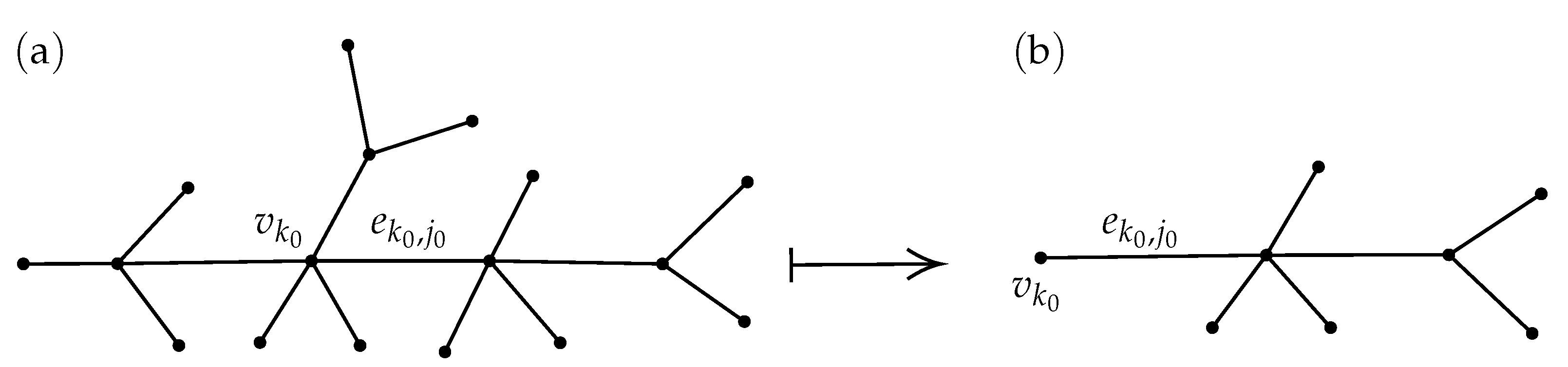
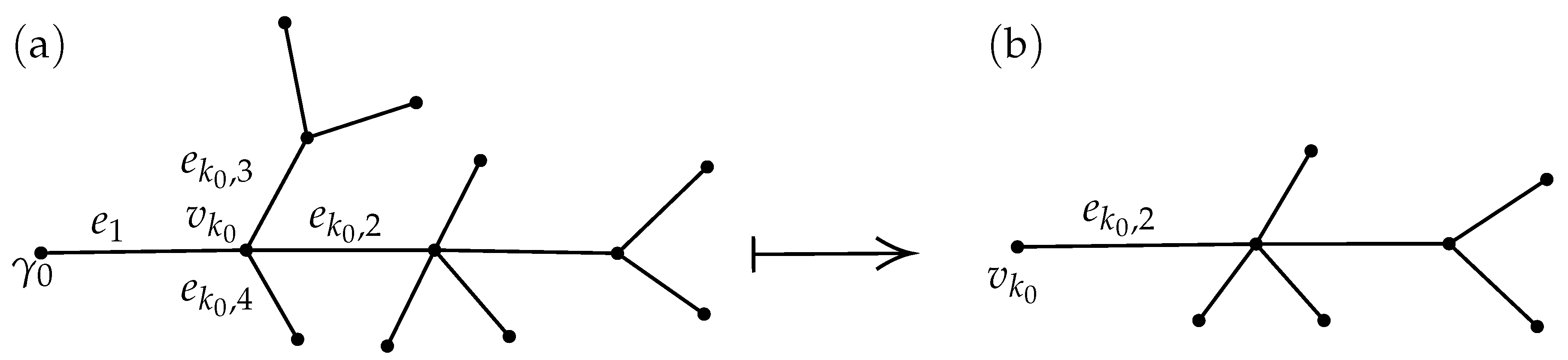
Now let $k_0$ be some fixed interior vertex, and let $j_0$ satisfy $1<j_0\le {\mathsf{{\rm Y}}}_{k_0}$. Denote by ${\mathsf{\Omega }}_{k_0}^{j_0}$ the unique subtree of $\mathsf{\Omega }$ having $v_{k_0}$ as root with incident edge $e_{k_0,j_0}$, and by $V_{k_0}^{j_0}$ the set of its vertices, see Figure 4.

We define an associated response operator as follows. Let ${\mathsf{\Gamma }}_{k_0}^{j_0}=\{v_{k_0},{\gamma }_{N_0},\dots ,{\gamma }_N\}$ be the boundary vertices on ${\mathsf{\Omega }}_{k_0}^{j_0}$. Suppose $\phi ={\phi }^b$ solves the IBVP

$$\frac{{\partial }^2\phi }{\partial t^2}-\frac{{\partial }^2\phi }{\partial x^2}+q\phi =0,x\in {\mathsf{\Omega }}_{k_0}^{j_0}\backslash V_{k_0}^{j_0},t\in \times [0,T],$$

(33)

$${\phi |}_{t=0}={{\phi }_t|}_{t=0}=0,$$

(34)

$$\partial \phi (v_k,t)=\partial {\phi }_j(v_k,t),j\in J\left(v_k\right),v_k\in V_{k_0}^{j_0}\backslash {\mathsf{\Gamma }}_{k_0}^{j_0},t\in [0,T],$$

(35)

$$\sum _{j\in J\left(v_k\right)}{\phi }_j(v_k,t)=0,v_k\in V_{k_0}^{j_0}\backslash {\mathsf{\Gamma }}_{k_0}^{j_0},t\in [0,T],$$

(36)

$$\partial \phi (v_{k_0},t)=b\left(t\right),t\in [0,T],$$

(37)

$$\phi ({\gamma }_l,t)=0,l=N_0,\dots ,N,t\in [0,T].$$

(38)

Then we define an associated reduced response operator

$$\left({\tilde{R}}_{k_0,j_0}b\right)\left(t\right)={\phi }_{j0}^b(v_{k_0},t),$$

with associated response function ${\tilde{R}}_{k_0,j_0}\left(s\right).$

Suppose we determined ${\tilde{R}}_{k_0,j_0}$. It would follow from Proposition 1 that one could recover the following data: ${\ell }_{j_0}$, $q_{j_0}$, and ${\mathsf{{\rm Y}}}_{k^{\prime }}$, where $v_{k^{\prime }}$ is the vertex adjacent to $v_{k_0}$ in ${\mathsf{\Omega }}_{k_0}^{j_0}$. In this section we will present an iterative method to determine the operator ${\tilde{R}}_{k_0,j_0}$ from the $\left(\right|\mathsf{\Gamma }|-1)$-tuple of operators, $R^T$, which we know by hypothesis for some $T<2\ell$. An important ingredient is the following generalization to a tree of Corollary 1.

Lemma 3.

Let $T<0$, and let $R_{k,j}^T$ be associated with (33)–(38), defined by (7) and (8). The response function for $R_{k,j}^T$ has the form

$$R_{k,j}\left(s\right)=r_{k,j}\left(s\right)+\sum _{n\ge 1}{\varphi }_{n}H(s-{\gamma }_n).$$

Here, $r_{k,j}\in {\mathcal{F}}^1$, and the sequence $\left\{{\gamma }_n\right\}$ is positive and strictly increasing. If T is finite then the sums are finite.

Proof. 

The proof follows from the proof of Corollary 1, together with the transmission and reflection properties of waves at interior vertices, and reflection properties at boundary vertices. □

Fix $T>2\ell$. The rest of this section shows how to recover ${\tilde{R}}_{k_0,j_0}$ from $R^T$.

Step 1

For the first step, let $v_{k_0}$ be the vertex adjacent to the root ${\gamma }_0$, with associated edge labeled $e_1$. By Proposition 1, we can use $R_{0,1}^T$ to recover ${\mathsf{{\rm Y}}}_{k_0}$, ${\ell }_1$, $q_1$.

Step 2

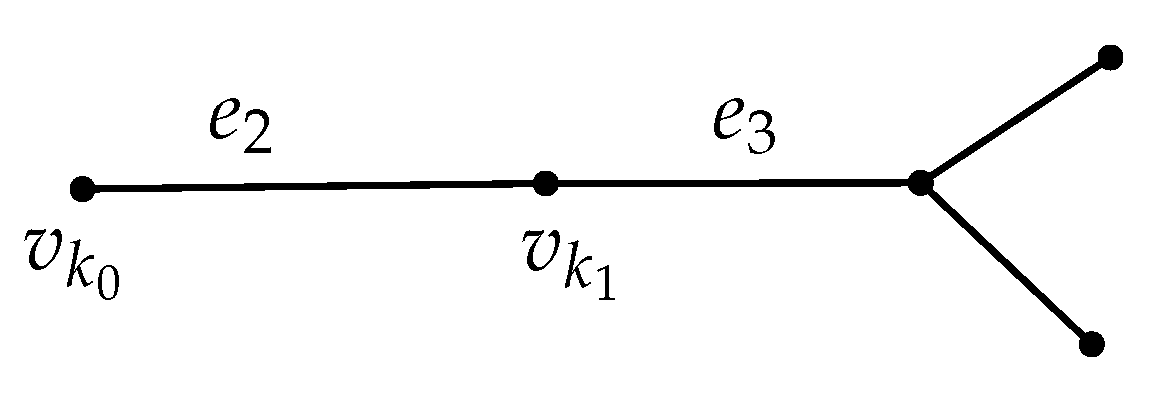
Consider $e_{k_0,2}$. In Step 2, we show how to solve for ${\tilde{R}}_{k_0,2}$, see Figure 5.

Since $v_{k_0}$ is the root of ${\mathsf{\Omega }}_{k_0}^2$, the following equation is essentially a restatement of Lemma 1 to trees; the details of its proof are left to the reader.

$${\tilde{R}}_{k_0,2}\left(s\right)={\tilde{r}}_{k_0,2}\left(s\right)+\sum _{m\ge 0}{\alpha }_{m}H(s-{\xi }_m).$$

(39)

Here, $0={\xi }_0<{\xi }_1<\dots$, and ${\tilde{r}}_{k_0,2}\left(s\right)\in {\mathcal{F}}^1$. In what follows in Step 2, for readability, we rewrite ${\tilde{r}}_{k_0,2}$ as $\tilde{r}$.

Since we know ${\ell }_1$ and $q_1$, we can solve the wave equation on $e_1$ with known boundary data. We identify $e_1$ as the interval $(0,{\ell }_1)$ with $v_{k_0}$ corresponding to $x=0$. Then $u^f$, restricted to $e_1$, solves the following Cauchy problem, where we view x as the “time” variable:

$$\begin{array}{ccc}\hfill u_{tt}-u_{xx}+q_{1}u& =& 0,x\in (0,{\ell }_1),t>0,\hfill \\ \hfill \partial u({\ell }_1,t)& =& f\left(t\right),t>0,\hfill \\ \hfill u({\ell }_1,t)& =& \left(R_{0,1}f\right)\left(t\right),t>0,\hfill \\ \hfill u(x,0)& =& 0,x\in (0,{\ell }_1).\hfill \end{array}$$

Since the function $R_{0,1}\left(s\right)$ is known, we can thus uniquely determine $u^f(0,t)=u^f(v_{k_0},t)$ and $\partial u_1^f(v_{k_0},t)$. Thus $p\left(t\right)=\partial u_2^{\delta }(v_{k_0},t)$ is determined.

We now show how p and $u_2^{\delta }(v_{k_0},t)$ can be used to determine ${\tilde{R}}_{k_0,2}\left(s\right)$. The following equation follows from the definition of the response operators for any $f\in L^2$:

$${\int }_0^t{\tilde{R}}_{k_0,2}\left(s\right)p(t-s)ds=u_2^{\delta }(v_{k_0},t)={\int }_0^t{R}_{k_0,2}\left(s\right)\delta (t-s)ds.$$

(40)

In what follows, it is convenient to extend $f\left(t\right)\in L^2(0,T)$ as zero for $t<0$. By Lemma 1 and by an adaptation of Lemma 2 to general trees, we have the following expansions:

$$\begin{array}{ccc}\hfill R_{k_0,2}\left(s\right)& =& r_{k_0,2}\left(s\right)+\sum _{n\ge 1}{\varphi }_{n}H(t-{\gamma }_n)r_{k_0,2}{|}_{s\in (0,{\beta }_1)}=0,{\beta }_1={\ell }_1,\hfill \end{array}$$

(41)

$$\begin{array}{ccc}\hfill p\left(s\right)& =& a(s-{\ell }_1)+\sum _{l\ge 1}{\psi }_l\delta (s-{\zeta }_l)+{\theta }_{l}H(s-{\zeta }_l),{\zeta }_1={\nu }_1={\ell }_1,{\psi }_1\ne 0,.\hfill \end{array}$$

(42)

Here, $r_{k_0,2}\in {\mathcal{F}}^1$ and $a\left(s\right)\in {\mathcal{F}}^1$, and $\left\{{\xi }_k\right\}$ and $\left\{{\beta }_n\right\}$ are positive and increasing. Clearly $a\left(s\right),r_{k_0,2}\left(s\right),\left\{{\psi }_m\right\},$$\left\{{\theta }_m\right\},$$\left\{{\varphi }_n\right\},$$\left\{{\gamma }_n\right\}$, can all be determined by $R_{0,1}$ and $R_{k_0,2}$, whereas for now $\tilde{r}$ and the sets $\left\{{\alpha }_m\right\},\left\{{\xi }_m\right\}$ are unknown. Inserting (39),(41) and (42) into (40), we get

$$\begin{array}{c}\hfill r_{k_0,2}\left(t\right)+\sum _n{\varphi }_{n}H(t-{\gamma }_n)={\int }_0^t\tilde{r}\left(s\right)a(t-s-{\ell }_1)ds+\sum _l{\psi }_l\tilde{r}(t-{\zeta }_l)+{\int }_0^t\sum _l{\theta }_{l}H(t-s-{\zeta }_l)\tilde{r}\left(s\right)ds\\ \hfill +\sum _m{\alpha }_m{\int }_0^{t}a(t-s-{\ell }_1)H(s-{\xi }_m)ds+\sum _{m,l}{\psi }_l{\alpha }_{m}H(t-{\zeta }_l-{\xi }_m)+\sum _{m,l}{\theta }_l{\alpha }_m{\int }_0^{t}H(s-{\xi }_m)H(t-s-{\zeta }_l)ds.\end{array}$$

(43)

Here all sums have 1 as lower limit of summation.

Lemma 4.

The sets $\left\{{\alpha }_m\right\},\left\{{\xi }_m\right\}$ can be determined by $R_{0,1}$ and $R_{k_0,2}$.

Proof. 

We mimic an iterative argument in [26]. Differentiating (43) and then matching the delta singularities, we get

$$\sum _{n\ge 1}{\varphi }_n\delta (t-{\gamma }_n)=\sum _{m\ge 1}\sum _{l\ge 1}{\psi }_l{\alpha }_m\delta (t-{\zeta }_l-{\xi }_m).$$

(44)

Since the sequences $\left\{{\gamma }_n\right\},\left\{{\zeta }_l\right\},\left\{{\xi }_m\right\}$ are all strictly increasing, clearly we have ${\gamma }_1={\zeta }_1+{\xi }_1$, so that ${\varphi }_1={\alpha }_1{\psi }_1$, and so ${\xi }_1={\gamma }_1-{\zeta }_1$ and ${\alpha }_1={\varphi }_1/{\psi }_1$. We represent that the set $\{{\varphi }_1,{\gamma }_1\},\{{\zeta }_1,{\psi }_1\}$ determines the set $\{{\xi }_1,{\alpha }_1\}$ by

$$\{{\varphi }_1,{\gamma }_1\},\{{\xi }_1,{\psi }_1\}\Rightarrow \{{\xi }_1,{\alpha }_1\}.$$

We now match the term $\delta (t-{\gamma }_2)$ with its counterpart on the right hand side of (44). There are three possible cases.

Case 1:${\gamma }_2\ne {\zeta }_2+{\xi }_1$.

In this case, we must have

$${\xi }_2={\gamma }_2-{\zeta }_1,{\alpha }_2={\varphi }_2/{\psi }_1.$$

Case 2a:${\gamma }_2={\zeta }_2+{\xi }_1$ and ${\varphi }_2\ne {\psi }_2{\alpha }_1.$ Note that the last inequality can be verified by an observer at this stage. Then ${\gamma }_2={\zeta }_1+{\xi }_2$ and ${\varphi }_2={\psi }_1{\alpha }_2+{\psi }_2{\alpha }_1.$ and hence

$${\xi }_2={\zeta }_1-{\gamma }_2,{\alpha }_2=({\varphi }_2-{\psi }_2{\alpha }_1)/{\psi }_1.$$

Case 2b:${\gamma }_2={\zeta }_2+{\xi }_1$ and ${\varphi }_2={\psi }_2{\alpha }_1.$ Then ${\gamma }_2\ne {\zeta }_1+{\xi }_2$. Note we have not yet solved for $\{{\xi }_2,{\alpha }_2\}$. In this case, we now repeat the matching coefficient argument just used with $\delta (t-{\gamma }_3)$.

Again there are three cases:

Case 2bi: ${\gamma }_3\ne {\zeta }_3+{\xi }_1$. Note all of these terms are known, so this inequality can be verified. In this case, ${\gamma }_3={\zeta }_1+{\xi }_2$, so ${\xi }_2={\gamma }_3-{\zeta }_1$ and ${\alpha }_2={\varphi }_3/{\psi }_1$.

Case 2bii: ${\gamma }_3={\zeta }_3+{\xi }_1$ and ${\varphi }_3\ne {\alpha }_1{\psi }_3$. Then ${\gamma }_3={\zeta }_1+{\xi }_2$, and ${\varphi }_3={\alpha }_1{\psi }_3+{\alpha }_2{\psi }_1$. Thus ${\xi }_2={\gamma }_3-{\zeta }_1$ and ${\alpha }_2=({\varphi }_3-{\alpha }_1{\psi }_3)/{\psi }_1$.

Case 2biii: ${\gamma }_3={\zeta }_3+{\xi }_1$ and ${\varphi }_3={\alpha }_1{\psi }_3$. Then ${\gamma }_3<{\zeta }_1+{\xi }_2$, and we need to continue our procedure with ${\gamma }_4$.

Repeating this procedure as necessary, say for a total of $N_2$ times, we solve for $\{{\xi }_2,{\alpha }_2\}$. We represent this process as

$${\{{\varphi }_k,{\gamma }_k\}}_{k=1}^{N_2}\Rightarrow {\{{\xi }_k,{\alpha }_k\}}_{k=1}^2.$$

We must have $N_2$ finite by (44) and the finiteness of the graph.

Iterating this procedure, suppose for $p\in \mathbb{N}$ we have

$${\{{\varphi }_k,{\gamma }_k\}}_{k=1}^{N_p}\Rightarrow {\{{\xi }_k,{\alpha }_k\}}_{k=1}^p.$$

Here $N_p$ is chosen to be minimal, and so ${\gamma }_{N_p}={\zeta }_1+{\xi }_p$. We wish to solve for $\{{\zeta }_{p+1},{\varphi }_{p+1}\}$.

We can again distinguish three cases:

Case 1:${\gamma }_{(N_p+1)}\ne {\zeta }_k+{\xi }_j,\forall j\le p,\forall k.$ Note that we know ${\left\{{\xi }_j\right\}}_1^p$ and $\left\{{\zeta }_k\right\}$, so these inequalities are verifiable. In this case, we must have ${\gamma }_{(N_p+1)}={\zeta }_1+{\xi }_{p+1}$ and ${\psi }_1{\alpha }_{p+1}={\varphi }_{(N_p+1)}$, so we have determined ${\alpha }_{p+1},{\xi }_{p+1}$ in this case.

Case 2: There exists an integer Q and pairs ${\{{\zeta }_{i_n},{\xi }_{j_n}\}}_{n=1}^Q$, with $j_n\le p$, such that

$${\gamma }_{(N_p+1)}={\zeta }_{i_1}+{\xi }_{j_1}=\dots ={\zeta }_{i_Q}+{\xi }_{j_Q}.$$

(45)

Note that all the numbers $\{{\zeta }_{i_n},{\xi }_{j_n}\}$ have been determined, so these equations can be all verified. We can assume all pairs $\{{\zeta }_{i_n},{\xi }_{j_n}\}$ satisfying (45) with $j_n\le p$ are listed. In this case, we have either

Case 2i: ${\varphi }_{(N_p+1)}\ne {\alpha }_{j_1}{\psi }_{i_1}+\dots +{\alpha }_{j_Q}{\psi }_{i_Q}.$ It follows then that ${\gamma }_{(N_p+1)}={\zeta }_1+{\xi }_{p+1}$, and

$${\varphi }_{(N_p+1)}={\alpha }_{p+1}{\psi }_1+{\varphi }_{j_1}{\psi }_{i_1}+\dots +{\varphi }_{j_Q}{\psi }_{i_Q}.$$

We thus solve for ${\xi }_{p+1},{\alpha }_{p+1}$.

Case 2ii: ${\gamma }_{(N_p+1)}={\varphi }_{j_1}{\psi }_{i_1}+\dots +{\varphi }_{j_Q}{\psi }_{i_Q}.$ It follows then that ${\alpha }_{(N_p+1)}\ne {\zeta }_1+{\xi }_{p+1}$, and we have to repeat this process with ${\gamma }_{(N_p+2)}$.

Repeating the reasoning in Case 2ii as often as necessary, we eventually solve for $\{{\xi }_{p+1},{\alpha }_{p+1}\}$. Thus,

$${\{{\varphi }_k,{\gamma }_k\}}_{k=1}^{N_{p+1}}\Rightarrow {\{{\xi }_k,{\alpha }_k\}}_{k=1}^{p+1}.$$

Hence, we can solve for $\{{\xi }_p:p\le L\},\{{\alpha }_p:p\le L\}$ for any positive integer L given knowledge of $R_{0,1}^T,R_{k_0,2}^T$ for $T=T\left(L\right)$ sufficiently large. □

It remains to solve for $\tilde{r}$. In what follows, we set $\tilde{R}\left(s\right)=0$ for $s<0$. We use $G\left(t\right)$ to denote various functions that we have already established to be determined by $R_{0,1}$ and $R_{k_0,2}$. Having already solved for $\{{\xi }_n,{\alpha }_n\}$, we can eliminate from (43) the Heavyside functions to get, recalling ${\zeta }_1={\ell }_1$,

$$G\left(t\right)=\sum _{l\ge 1}{\psi }_l\tilde{r}(t-{\zeta }_l)+{\int }_0^t\tilde{r}\left(s\right)(a(t-s-{\zeta }_1))+\sum _{l\ge 1}{\theta }_{l}H(t-s-{\zeta }_l)ds.$$

(46)

We solve this with an iterative argument. Let $\alpha ={min}_m\{{\zeta }_{l+1}-{\zeta }_l\}$. For $t<{\zeta }_1+\alpha$, we have for $l>1$ that $t-{\zeta }_l<0$ so $r\left(t\right)=0$. Hence

$$G\left(t\right)={\psi }_1\tilde{r}(t-{\zeta }_1)+{\int }_0^t\left({\theta }_{1}H(t-s-{\zeta }_1)+a(t-s-{\zeta }_1)\right)\tilde{r}\left(s\right)ds,t<{\zeta }_1+\alpha .$$

(47)

Letting $r=t-{\zeta }_1$, we get

$$\begin{array}{ccc}\hfill G\left(r\right)& =& {\psi }_1\tilde{r}\left(r\right)+{\int }_0^{r+{\zeta }_1}\left({\theta }_{1}H(r-s)+a(r-s)\right)\tilde{r}\left(s\right)ds,\hfill \\ & =& {\psi }_1\tilde{r}\left(r\right)+{\int }_0^r\left({\theta }_{1}H(r-s)+a(r-s)\right)\tilde{r}\left(s\right)ds,r<\alpha .\hfill \end{array}$$

We solve this VESK to determine $\tilde{r}\left(s\right),r<\alpha$. Now for $t<{\zeta }_1+2\alpha$, we have for $l>1$ that $t-{\zeta }_l<\alpha$, and so those terms in (46) with $t-{\zeta }_l$ can be absorbed in G to again give

$$G\left(r\right)={\psi }_1\tilde{r}\left(r\right)+{\int }_0^r\left({\theta }_{1}H(r-s)+a(r-s)\right)\tilde{r}\left(s\right)ds,r<2\alpha .$$

We solve this VESK to determine $\tilde{r}\left(s\right),r<2\alpha$. Iterating this procedure, we solve for $\tilde{r}\left(s\right)$ for any finite s.

Step 3 Because $R_{k_0,j}$ are determined by assumption for $j=2,\dots ,{\mathsf{{\rm Y}}}_{k_0}-1$, the functions $u_j^f(v_{k_0},t)$ are determined. In Step 2, we showed $u_1^f(v_{k_0},t)$ is also determined. Hence by (4), $u_{{\mathsf{{\rm Y}}}_{k_0}}^f(v_{k_0},t)$ is also determined. We can now carry out the argument in Step 2 on the remaining edges $e_{k_0,3},\dots ,e_{k_0,{\mathsf{{\rm Y}}}_{k_0}}$ incident on $v_{k_0}$ to determine ${\tilde{R}}_{k_0,j}$ for all j.

Step 4 For each $j=2,\dots ,{\mathsf{{\rm Y}}}_{k_0}$, we use Proposition 1, to find the associated ${\ell }_j,q_j$ together with the valence of the vertex adjacent to $v_{k_0}$. Careful reading of Steps 2 and 3 shows that we can use $R_{0,1}^T$ and $R_{k_0,j}^T$ for any $T>2({\ell }_1+{\ell }_j)$.

Step 5 Let $v_{k_1},\dots$ be the vertices adjacent to $v_{k_0}$, other than ${\gamma }_0$. We now iterate Steps 2–4 for the each of these vertices. Choose for instance $v_{k_1}$. If it were a boundary vertex, this fact would be determined in Step 4, and then this algorithm goes to the next vertex, which we, for convenience, still label $v_{k_1}$. We can thus assume $v_{k_1}$ is an interior vertex. Let us label an incident edge (other than $e_2:=e_{k_0,2}$) as $e_3:=e_{k_1,3}$, see Figure 6.

We wish to determine ${\tilde{R}}_{k_1,3}$. Mimicking Step 2, let $u^{\delta }$ solve (1)–(6), let $b\left(t\right)=\partial u_3^{\delta }(v_{k_1},t)$. We have the following formula holding by the definition of response operators:

$${\int }_0^t{\tilde{R}}_{k_1,3}\left(s\right)b(t-s)ds={\int }_0^t{R}_{k_1,3}\left(s\right)\delta (t-s)ds.$$

Of course $R_{k_1,3}\left(s\right)$ is assumed to be known. We determine b as follows. We have, from Step 2, that $p\left(t\right)=\partial u_1^{\delta }(v_{k_0},t)$ is known. We identify $e_2$ as the interval $(0,{\ell }_2)$ with $v_{k_1}$ corresponding to $x=0$.

Then $b\left(t\right)=\partial u_2^f(v_{k_1},t)$ arises as a solution to the following Cauchy problem on $e_2$, where we view x as the “time” variable:

$$\begin{array}{ccc}\hfill y_{tt}-y_{xx}+q_{2}y& =& 0,x\in (0,{\ell }_2),t>0\hfill \\ \hfill y_x({\ell }_2,t)& =& p\left(t\right),t>0\hfill \\ \hfill y({\ell }_2,t)& =& \left(R_{k_0,2}\delta \right)\left(t\right),t>0\hfill \\ \hfill y(x,0)& =& 0,x\in (0,{\ell }_2).\hfill \end{array}$$

Since $q_2,{\ell }_2,$ and $R_{k_0,2}$ are all known, we can thus determine $b\left(t\right)=y_x(0,t)$.

The rest of the argument here is a straightforward adaptation of Steps 2–4 above. The details are left to the reader.

Step 6 Arguing as in Step 5, we determine ${\tilde{R}}_{k,j}$ for all other vertices adjacent to $v_{k_0}$ and their associated edges. The details are left to the reader.

Steps above 6 Clearly this procedure can be iterated until all edges of our finite graph have been covered.

5. Conclusions

In this paper, we applied the ideas of the boundary control and leaf peeling methods to solve an inverse problem on a tree featuring non-standard, delta-prime vertex conditions on the interior. Our method required using only one boundary actuator and one boundary sensor, all other observations being internal. Using the Neumann-to-Dirichlet map (acting from one boundary vertex to one boundary and all internal vertices) we recovered the topology and geometry of the graph together with the coefficients $q_j$ of the equations. It would be interesting to see a numerical implementation of our method. It would also be interesting to adapt our methods to quantum graphs with cycles.

References

- Lagnese, J.; Leugering, G.; Schmidt, E.J.P.G. Modelling, Analysis, and Control of Dynamical Elastic Multilink Structures; Birkhauser: Basel, Switzerland, 1994. [Google Scholar]
- Gugat, M.; Leugering, G. Global boundary controllability of the Saint-Venant system for sloped canals with friction. Ann. Inst. H. Poincaré Anal. Non Lineaire 2009, 26, 257–270. [Google Scholar] [CrossRef] [Green Version]
- Alì, G.; Bartel, A.; Günther, M. Parabolic Differential-Algebraic Models in Electrical Network Design. Multiscale Model. Simul. 2005, 4, 813–838. [Google Scholar] [CrossRef]
- Bastin, G.; Coron, J.M.; dÁndrèa Novel, B. Using hyperbolic systems of balance laws for modeling, control and stability analysis of physical networks. In Proceedings of The Lecture Notes for the Pre-Congress Workshop on Complex Embedded and Networked Control Systems 17th IFAC World Congress, Seoul, Korea, 16–20 July 2008; Elsevier: Amsterdam, The Netherlands, 2008. [Google Scholar]
- Colombo, R.M.; Guerra, G.; Herty, M.; Schleper, V. Optimal control in networks of pipes and canals. SIAM J. Control Optim. 2009, 48, 2032–2050. [Google Scholar] [CrossRef]
- Hurt, N.E. Mathematical Physics of Quantum Wires and Devices; Kluwer: Dordrecht, The Netherlands, 2000. [Google Scholar]
- Joachim, C.; Roth, S. (Eds.) Atomic and Molecular Wires; NATO Science Series. Series E: Applied Sciences; Kluwer: Dordrecht, The Netherlands, 1997; p. 341. [Google Scholar]
- Kostrykin, V.; Schrader, R. Kirchoff’s rule for quantum wires. J. Phys. A Math. Gen. 1999, 32, 595–630. [Google Scholar] [CrossRef]
- Kostrykin, V.; Schrader, R. Kirchoff’s rule for quantum wires II: The inverse problem with possible applications to quantum computers. Fortschritte Derphysik 2000, 48, 703–716. [Google Scholar] [CrossRef] [Green Version]
- Kottos, T.; Smilansky, U. Quantum chaos on graphs. Phys. Rev. Lett. 1997, 79, 4794–4797. [Google Scholar] [CrossRef]
- Kottos, T.; Smilansky, U. Periodic orbit theory and spectral statistics for quantum graphs. Ann. Phys. 1999, 274, 76–124. [Google Scholar] [CrossRef] [Green Version]
- Melnikov, Y.B.; Pavlov, B.S. Two-body scattering on a graph and application to simple nanoelectronic devices. J. Math. Phys. 1995, 36, 2813–2825. [Google Scholar] [CrossRef] [Green Version]
- Adam, S.; Hwang, E.H.; Galits, V.M.; Das Sarma, S. A self-consistent theory for graphene transport. Proc. Natl. Acad. Sci. USA 2007, 104, 18392–18397. [Google Scholar] [CrossRef] [Green Version]
- Peres, N.M.R. Scattering in one-dimensional heterostructures described by the Dirac equation. J. Phys. Condens. Matter 2009, 21, 095501. [Google Scholar] [CrossRef] [Green Version]
- Peres, N.M.R.; Rodrigues, J.N.B.; Stauber, T.; Lopes dos Santos, J.M.B. Dirac electrons in graphene-based quantum wires and quantum dots. J. Phys. Condens. Matter 2009, 21, 344202. [Google Scholar] [CrossRef] [PubMed] [Green Version]
- Avdonin, S.A.; Bell, J. Determining a distributed conductance parameter for a neuronal cable model defined on a tree graph. Inverse Probl. Imaging 2015, 9, 645–659. [Google Scholar] [CrossRef]
- Bell, J.; Craciun, G. A distributed parameter identification problem in neuronal cable theory models. Math. Biosci. 2005, 194, 1–19. [Google Scholar] [CrossRef] [PubMed]
- Rall, W. Core conductor theory and cable properties of neurons. In Handbook of Physiology, The Nervous System; American Physiological Society: Rockville, MD, USA, 1977; pp. 39–97. [Google Scholar]
- Berkolaiko, G.; Kuchment, P. Introduction to Quantum Graphs, (Mathematical Surveys and Monographs; American Mathematical Society: Providence, RI, USA, 2013; Volume 186. [Google Scholar]
- Exner, P. Vertex couplings in quantum graphs: Approximations by scaled Schrödinger operators. In Mathematics in Science and Technology; World Sci. Publ.: Hackensack, NJ, USA, 2011; pp. 71–92. [Google Scholar]
- Avdonin, S.A.; Kurasov, P. Inverse problems for quantum trees. Inverse Probl. Imaging 2008, 2, 1–21. [Google Scholar] [CrossRef]
- Al-Musallam, F.; Avdonin, S.A.; Avdonina, N.; Edward, J. Control and inverse problems for networks of vibrating strings with attached masses. Nanosyst. Phys. Chem. Math. 2016, 7, 835–841. [Google Scholar] [CrossRef] [Green Version]
- Avdonin, S.A.; Avdonina, N.; Edward, J. Boundary inverse problems for networks of vibrating strings with attached masses. In Proceedings of the Dynamic Systems and Applications, Volume 7, Dynamic, Atlanta, GA, USA, 27–30 May 2015; pp. 41–44. [Google Scholar]
- Avdonin, S.A.; Mikhaylov, V.S.; Nurtazina, K.B. On inverse dynamical and spectral problems for the wave and Schrödinger equations on finite trees. The leaf peeling method. J. Math. Sci. 2017, 224, 1–15. [Google Scholar] [CrossRef] [Green Version]
- Avdonin, S.A.; Zhao, Y. Leaf peeling method for the wave equation on metric tree graphs. Inverse Probl. Imaging 2020. [Google Scholar] [CrossRef]
- Avdonin, S.A.; Edward, J. An inverse problem for quantum trees. 2020. submitted. [Google Scholar] [CrossRef]
- Avdonin, S.A.; Zhao, Y. Exact controllability of the 1-d wave equation on finite metric tree graphs. Appl. Math. Optim. 2020. [Google Scholar] [CrossRef]
- Avdonin, S.A. Control problems on quantum graphs. In Analysis on Graphs and Its Applications (Proceedings of Symposia in Pure Mathematics); AMS: Pawtucket, RI, USA, 2008; Volume 77, pp. 507–521. [Google Scholar]
- Avdonin, S.A.; Nicaise, S. Source identification problems for the wave equation on graphs. Inverse Probl. 2015, 31, 095007. [Google Scholar] [CrossRef]
- Belishev, M.I.; Vakulenko, A.F. Inverse problems on graphs: Recovering the tree of strings by the BC-method. J. Inverse Ill-Posed Probl. 2006, 14, 29–46. [Google Scholar] [CrossRef]
- Dager, R.; Zuazua, E. Wave Propagation, Observation and Control in 1-d Flexible Multi-Structures, (Mathematiques and Applications); Springer: Berlin/Heidelberg, Germany, 2006; Volume 50. [Google Scholar]
- Avdonin, S.A.; Kurasov, P.; Nowaczyk, M. Inverse problems for quantum trees II: On the reconstruction of boundary conditions for star graphs. Inverse Probl. Imaging 2010, 4, 579–598. [Google Scholar] [CrossRef]
- Avdonin, S.A.; Edward, J. Controllability for string with attached masses and Riesz bases for asymmetric spaces. Math. Control Relat. Fields 2019, 9, 453–494. [Google Scholar] [CrossRef] [Green Version]
Figure 1.
A metric tree.
Figure 2.
Sensors at vertex marked by arrows.
Figure 3.
Star with coordinate system: identified with .
Figure 4.
(a) , (b) Subtree .
Figure 5.
(a) . (b) Subtree , with .
Figure 6.
For Step 5: a subtree of .
Publisher’s Note: MDPI stays neutral with regard to jurisdictional claims in published maps and institutional affiliations. |
© 2020 by the authors. Licensee MDPI, Basel, Switzerland. This article is an open access article distributed under the terms and conditions of the Creative Commons Attribution (CC BY) license (http://creativecommons.org/licenses/by/4.0/).
Share and Cite
MDPI and ACS Style
Avdonin, S.; Edward, J. An Inverse Problem for Quantum Trees with Delta-Prime Vertex Conditions. Vibration 2020, 3, 448-463. https://0-doi-org.brum.beds.ac.uk/10.3390/vibration3040028
AMA Style
Avdonin S, Edward J. An Inverse Problem for Quantum Trees with Delta-Prime Vertex Conditions. Vibration. 2020; 3(4):448-463. https://0-doi-org.brum.beds.ac.uk/10.3390/vibration3040028
Chicago/Turabian StyleAvdonin, Sergei, and Julian Edward. 2020. "An Inverse Problem for Quantum Trees with Delta-Prime Vertex Conditions" Vibration 3, no. 4: 448-463. https://0-doi-org.brum.beds.ac.uk/10.3390/vibration3040028