Article

Comparison of Reduction Methods for Finite Element Geometrically Nonlinear Beam Structures

1
Institut of Mechanical Sciences and Industrial Applications (IMSIA), ENSTA Paris, CNRS, EDF, CEA, Institut Polytechnique de Paris, 91762 Palaiseau, France
2
Vibration University Technology Centre, Imperial College London, London SW7 2AZ, UK
3
Arts et Métiers Institute of Technology, LISPEN, HESAM Université, 8 boulevard Louis XIV, 59000 Lille, France
*
Author to whom correspondence should be addressed.
Submission received: 13 January 2021 / Revised: 18 February 2021 / Accepted: 1 March 2021 / Published: 4 March 2021
(This article belongs to the Special Issue Model Order Reduction of Nonlinear Systems)

Abstract

:
The aim of this contribution is to present numerical comparisons of model-order reduction methods for geometrically nonlinear structures in the general framework of finite element (FE) procedures. Three different methods are compared: the implicit condensation and expansion (ICE), the quadratic manifold computed from modal derivatives (MD), and the direct normal form (DNF) procedure, the latter expressing the reduced dynamics in an invariant-based span of the phase space. The methods are first presented in order to underline their common points and differences, highlighting in particular that ICE and MD use reduction subspaces that are not invariant. A simple analytical example is then used in order to analyze how the different treatments of quadratic nonlinearities by the three methods can affect the predictions. Finally, three beam examples are used to emphasize the ability of the methods to handle curvature (on a curved beam), 1:1 internal resonance (on a clamped-clamped beam with two polarizations), and inertia nonlinearity (on a cantilever beam).

1. Introduction

Model reduction methods have been investigated for a long time for thin structures experiencing large-amplitude vibrations with geometric nonlinearities [1,2]. The two main identified difficulties are that the nonlinearity is distributed, and that the dynamical phenomena displayed by these nonlinear vibrations are numerous, including jump phenomena [3], bifurcations of solutions [4,5], internal resonance and modal interactions [6,7,8,9], strong couplings [10], transition to chaos [11,12], and wave turbulence [13]. Consequently, deriving accurate and predictive reduced-order models (ROMs) requires tackling these two problems in such a manner that the possible dynamics of the ROM can mimic all of the complexity of the full-order solution. In this contribution, only the nonlinear reduction methods, where a curved subspace is derived as a reduction manifold and/or a nonlinear mapping is used, are considered. All of the linear methods based on optimal orthogonal basis selection, such as Proper Orthogonal Decomposition (POD), are not taken into account in the discussion and comparisons, since they have already been covered in numerous articles. The interested reader is referred, e.g., to [14,15,16,17,18,19] and references therein for the literature on these linear methods.
Focusing on the nonlinear methods, the first steps can be traced back to the pioneering work by Shaw and Pierre, who introduced invariant manifolds—tangent at the origin to the linear eigensubspaces—as nonlinear normal modes (NNMs) of the vibrating structures [20,21]. Using a technique used to compute the center manifold from dynamical systems theory [22,23], they proposed a general methodology that is applicable for model-order reduction of vibratory systems, which has been applied successfully on a number of examples [24,25,26]. Later on, the normal form approach, which is also a key feature of the general theory of dynamical systems, was applied to vibratory systems with the aim of proposing a method for model-order reduction [27,28,29]. In particular, the method generalizes the development led by Shaw and Pierre by proposing a full third-order nonlinear mapping, allowing one to pass from the modal coordinates to an invariant-based span of the phase space. Applications to shell problems demonstrated the ability of the method to propose efficient ROMs that are able to capture important dynamical phenomena, such as 1:1 resonance [19,28,30]. A recent development generalizes the notion of invariant manifolds and NNMs in order to propose a mathematically well-justified framework, allowing one to tackle conservative as well as dissipative systems. Spectral submanifolds (SSMs) were introduced in [31], and their use in model reduction was emphasized with different applications [32,33,34,35] to underline the accuracy of the method.
Most of the tools presented in the previous paragraph emerged from the dynamical system theory and were scarcely applied to finite element (FE)-based methods, probably because of the large size of the models. Moreover, the intensive use of industrial numerical codes in engineering applications led to the problem of using them in a non-intrusive manner, i.e., without the need to enter at the elementary level to derive the reduction method, but instead using the standard procedures and outputs of a general code to produce an ROM [36]. In this realm, the stiffness evaluation procedure (STEP), first proposed in [37] and then extended in [38], allows direct computation of the modal nonlinear coupling coefficients of a modal ROM from a set of prescribed displacements and simple algebra. However, one can note that, as such, STEP is not a reduction method, since it only offers a method to efficiently compute these coupling coefficients, without solving the issue of selecting the relevant modes of the ROM or reducing its size. On the other hand, the implicit condensation and expansion (ICE) method was introduced in [39,40,41,42]. In this case, a set of prescribed loads is used to construct a so-called stress manifold, which is then fitted in order to derive the ROM [43,44]. More recently, modal derivatives and their extension with the definition of a nonlinear mapping were used to create a quadratic manifold (QM) approach, which was derived in [45,46].
Keeping in mind their non-intrusive characteristics, applications of the methods from dynamical system theory to the peculiarity of FE-based procedures have recently been further investigated. In [47], a third-order general method was derived, whose formula allowed retrieval of the invariant manifold approach proposed by Shaw and Pierre. On the other hand, the normal form approach was adapted to the FE context in [48]. In this last contribution, a special emphasis was put on how to use the method in a non-intrusive manner in order to create accurate ROMs from the FE mesh, including forcing and damping. The method was named DNF (direct normal form).
A comparison of the ICE and QM methods with invariant manifold and spectral submanifolds was proposed in [49,50,51], showing that from the theoretical point of view, the first two methods need a slow/fast assumption between the master and slave coordinates to propose accurate ROMs. In this contribution, the comparison is put not on the theoretical basis of the methods, but rather on the given results, and numerous beam cases discretized with the FE procedure are used as illustrative examples. A particular emphasis is put on comparing the ICE method, the QM method—using either full modal derivatives (MDs) or their simplified versions, called static modal derivatives (SMDs)—and the DNF approach.
The paper is organized as follows. In Section 2, the general framework of a geometrically nonlinear structure with the FE procedure is first recalled in Section 2.1; then, the three reduction methods to be compared are reviewed. The ICE method is briefly sketched in Section 2.2, the QM method using MDs and SMDs is described in Section 2.3, and the DNF approach is detailed in Section 2.4. Section 2 closes with an analytical example used in Section 2.5—a linear beam resting on a nonlinear elastic foundation—clearly illustrating the advantages and shortcomings of the different methods. Section 3 investigates three different beam examples discretized with the FE method. Section 3.1 first considers the case of a clamped–clamped beam with increasing curvature, transforming a straight beam into a non-shallow arch. Section 3.2 considers the two polarizations of a straight clamped–clamped beam, thus tackling the case of 1:1 internally resonant dynamics where two master modes are needed. Finally, Section 3.3 considers the case of a cantilever beam. Conclusions are drawn in Section 4.

2. Reduced-Order Models for Finite Element Structures

In this section, the three reduction methods that will be compared are introduced in the general framework of finite element structures with geometric nonlinearity. The next section recalls the general background and starting equations.

2.1. Theoretical Framework

A continuous structure, semi-discretized in space with the finite element (FE) method, is considered. Since our interest is in large-amplitude vibrations, geometric nonlinearities are included in the model with a nonlinear Green–Lagrange relationship between strains and displacements. The constitutive law is linear elastic, of the Saint–Venant–Kirchhoff type [52,53,54]. The starting point is thus the equations of motion written in the physical basis for the N-dimensional vector u of generalized displacements at the nodes, where N is the number of degrees of freedom (dofs) of the FE problem. The semi-discrete, finite-dimensional equation of motion reads:
M u ¨ + C u ˙ + F ( u ) = Q ,
where M is the mass matrix, C is the damping matrix, F ( u ) represents the nonlinear restoring force, and Q represents the external force. In this contribution, the case of Rayleigh damping will be specifically considered, as commonly used in an FE context, so that one can specify for the damping matrix C = ζ M M + ζ K K , where ζ M and ζ K are two coefficients to be selected. In the context of geometrically nonlinear structures, the nonlinear part of the stiffness is polynomial and contains only quadratic and cubic terms [36,54,55], such that the restoring force is expressed as:
F ( u ) = K u + G ( u , u ) + H ( u , u , u ) ,
where K is the tangent stiffness matrix, and G and H represent, respectively, the quadratic and cubic terms. Detailed indicial expressions of G and H are reported in Appendix A for the sake of completeness. For the next developments, the linear mode basis needs to be introduced. The eigenmode shape ϕ i and its corresponding eigenfrequency ω i are solutions of
K ω i 2 M ϕ i = 0 .
The equations of motion (1) can be rewritten in the modal space using the linear change of coordinates u = P ϕ X , where P ϕ is the matrix of eigenvectors ϕ i and X represents the modal coordinates. After projection, the dynamics read
X ¨ + Ω 2 X + D X ˙ + g ( X , X ) + h ( X , X , X ) = F ,
where Ω 2 stands for the diagonal matrix composed of squared eigenfrequencies, while g and h are the quadratic and cubic terms expressed in the modal basis [37,54], the detailed expressions of which are given in Appendix A. The diagonal damping matrix in the modal basis reads D = P ϕ T C P ϕ , and the external force vector reads F = P ϕ T Q .
Reduction methods are needed in an FE context, since the number of dofs N can be prohibitively large, preventing either direct calculation of Equation (1) or the possibility of building the problem in modal space, as in Equation (4). Due to the geometric nonlinearity, nonlinear terms G and H create important couplings among dofs and among modes, which impede simple analyses or even simple truncation schemes based on linear ideas using, e.g., the frequency content of the input force Q . Consequently, numerous methods have been proposed in the past in order to reduce Equation (1) to a smaller subset of well-selected master coordinates. The next sections present three of these methods that will be compared and evaluated on dedicated beam examples.

2.2. Implicit Condensation and Expansion

The implicit condensation and expansion (ICE) method was first introduced by McEwan, Gordon, and Hollkamp [39,40,41,42], and was recently used by Kuether et al. [44] and Frangi and Gobat [43]. It is sometimes also called the applied force method (AMF), since it relies on applying a set of selected static forces on the FE model as a first step for deriving the ROM. This is in contrast with the stiffness evaluation procedure (STEP), which applies a set of prescribed static displacements to the structure from which, following simple algebra, the quadratic and cubic modal coupling coefficients, g i j p and h i j k p , can be deduced [37,38]. On the other hand, for the ICE method, a stress manifold is built from the set of prescribed applied loads [43]. This explains, in particular, why the coefficients from the ICE method strongly depend on the amplitude of the applied load, since they follow the curvature of the stress manifold, while the modal coupling coefficients of the STEP do not depend on the amplitude of the applied displacement on a large interval, since linear modal eigenspaces are not curved [51,55].
Let us briefly recall the main steps needed for deriving the ICE method. The interested reader is referred to [42,43,51] for further details. The first step is to impose body forces Q that are proportional to the inertia of a number of selected linear modes, Q = β i M ϕ i in Equation (1), with i = 1 m , m being the number of master coordinates retained in the ROM. A static problem is then solved with the FE code, and the obtained displacement field is projected onto the eigenmodes in order to get the modal displacements X p corresponding to the imposed force for p = 1 m . A mapping is thus constructed with entries β i and outputs X p . Assuming that the functional relationship is invertible, one obtains X p ( β i ) , from which the ROM can be built. At the last step, a fitting procedure is executed in order to derive functional forms from the computed clouds of points to obtain the β ( X ) from the the map X ( β ) .
The reduced-order dynamics derived by the ICE method are m-dimensional and read:
X ¨ + Ω 2 X + D X ˙ + β ( X ) = F ,
One main advantage is that the method implicitly takes into account the axial-bending nonlinear coupling that causes geometric nonlinearities; it is thus particularly appealing when working with thin, flat structures. The main drawback of the method is the fact that a fitting procedure is needed after application of the forces in order to get the nonlinear restoring force on the stress manifold. If this is not problematic when working with a single master coordinate, the inclusion of more and more master modes makes the method difficult to implement in a general m-dimensional case. More importantly, the method then becomes very sensitive to the values of the applied loads [51]. As shown in [51], the implicit condensation can never perform better than the usual static condensation, so one cannot expect to obtain better results than with the use of static condensation. A quantitative and analytic comparison with the invariant manifold approach also underlines that the stress manifold is not an invariant subspace, and that ICE can give reliable results only in cases where a slow/fast approximation exists between master and slave coordinates [49,51]. This slow/fast approximation refers to the case where the eigenfrequencies of the slave modes are very large as compared to those of the master modes, ensuring that the slave coordinates display much stiffer dynamics. A formal demonstration of this result is given in [49] as a theorem, and a practical rule to apply the slow/fast approximation was given in [51] by stating that the frequency gap between slave and master eigenfrequencies should be larger than 6 to get reliable results.

2.3. Quadratic Manifold with Modal Derivatives

In this section, the quadratic manifold (QM) method based on modal derivatives, which was first introduced in [45,46], is presented. The main idea is to derive a nonlinear mapping by using the modal derivatives as a quadratic dependence on the master coordinates to pass from the FE nodes to a reduced subspace built on a quadratic manifold. In a first subsection, we recall the definition of modal derivatives and then explain how the quadratic manifold is built from them. The presentation summarizes a general development shown in [50], where the QM method was compared to the normal form approach.

2.3.1. Definition of Full and Static Modal Derivatives

Modal derivatives were first introduced in [56] with the idea of accounting for the variation in the eigenmodes with amplitude. In that respect, let us denote as ϕ ˜ i ( u ) the amplitude-dependent eigenvector. The i j -th modal derivative Θ ij is thus introduced as the derivative of ϕ ˜ i with respect to the j-th coordinate used for the reduced basis, so that one can write [45,46,50,57]:
Θ ij ϕ i ˜ ( u ) X j | u = 0 .
In order to derive an explicit problem of which the MD will be the solution, it is convenient to rewrite the eigenvalue system defined in Equation (3) and to state the explicit dependence of the mode shape and eigenfrequency on the amplitude u , thus obtaining:
F ( u ) u ω ˜ i 2 ( u ) M ϕ ˜ i ( u ) = 0 ,
where the tangent stiffness matrix K has been replaced by the derivative of the full nonlinear restoring force F with respect to the amplitude. Note also that it has been assumed that the mass matrix is not amplitude-dependent. Expanding Equation (7) in Taylor series for small vibrations, one can observe that the first term will reproduce the usual linear eigenproblem, while the next term will make the modal derivative Θ ij appear. Since the frequency’s dependence on amplitude also appears, a second equation is used to close the problem, and the developments shown in [45,46,57] advocate for the use of the mass normalization equation: ϕ ˜ i T M ϕ ˜ i = 1 . Expanding in Taylor series also produces a second equation; finally, grouping the two gives the system from which one can compute the MD:
K ω i 2 M M ϕ i ϕ i T M 0 Θ ij ω i 2 X j = 2 G ( ϕ j , ϕ i ) 0 .
The solution of Equation (8) is generally difficult to obtain because of the singularity of the K ω i 2 M in the eigenmode directions. In addition, obtaining all the terms in Equation (8) with FE software is not straightforward, since some of them do not correspond to standard operations. Consequently, most of the results found in the literature on MDs simplify the problem given by Equation (8) by neglecting the inertia, thus defining the so-called static modal derivatives (SMDs), which are the solution of the simpler problem:
K Θ ij = 2 G ( ϕ j , ϕ i ) .
As remarked in [45,46,50], the computation of these SMDs can be performed in a non-intrusive manner with a standard FE code.

2.3.2. Reduction with the Quadratic Manifold

The modal derivatives were first introduced with the aim of completing the linear mode basis with additional vectors (MDs) in order to take into account the new spanning directions given by the curvature of the invariant manifold in phase space, and have been used as such in numerous contexts; see, e.g., [58]. However, it then appeared logical to embed these added vectors in a nonlinear mapping. Indeed, from the definition of the modal derivatives, it is possible to define a nonlinear mapping from the initial physical dofs to the master coordinates, stating that the quadratic part of the mapping is conveyed by the introduced MDs or SMDs. Following [45,46,50], one can write such a relationship in a compact form as
u = Ξ ( X ) = Φ X + 1 2 Θ ¯ ( X , X ) = i = 1 m ϕ i X i + 1 2 i = 1 m j = 1 m Θ ¯ i j X i X j ,
where Ξ stands for the quadratic nonlinear mapping, and Φ is the N × m matrix of the master eigenvectors only, i.e., it is the restriction of P ϕ to the m selected master modes; Θ ¯ i j = ( Θ i j + Θ j i ) / 2 is the symmetrized MD. The reduced-order dynamics are obtained by applying the second-order nonlinear mapping (10) to the original equations of motion (1). For that purpose, one can introduce the tangent space of the manifold P Ξ as [45,46]:
P Ξ = Ξ X
where P Ξ is a matrix whose k-th column [ P Ξ ] k is written as
[ P Ξ ] k = Ξ X k = ϕ k + j = 1 m Θ ¯ j k X j .
Deriving (10) two times with respect to t leads to:
u ˙ = Ξ ˙ = P Ξ X ˙ ,
u ¨ = Ξ ¨ = P Ξ X ¨ + P Ξ X X ˙ X ˙ .
Substituting for these in Equation (1), the reduced-order dynamics read:
P Ξ t M Ξ ¨ + P Ξ t C Ξ ˙ + P Ξ t K Ξ + P Ξ t G ( Ξ , Ξ ) + P Ξ t H ( Ξ , Ξ , Ξ ) = P Ξ t Q .
One can note, in particular, that the quadratic and cubic terms G ( Ξ , Ξ ) and H ( Ξ , Ξ , Ξ ) will produce higher orders (up to power four for the first and power six for the second), and these higher orders will not be balanced by additional terms being taken into account in the nonlinear mapping, which is a common feature in such asymptotic developments. Consequently, it might appear more reasonable to also truncate Equation (14) to the third order to maintain consistency. Following [50], one finally obtains, in full indicial notation, and by including Rayleigh damping, the third-order reduced dynamics, reading p = 1 , , m :
X ¨ p + ω p 2 X p + ( ζ M + ζ K ω p 2 ) X ˙ p + i , j = 1 m ( g i j p + ω p 2 2 θ ¯ i j p ) X i X j + θ ¯ i j p ( X ˙ i X ˙ j + X i X ¨ j ) + θ ¯ p i j ( ω j 2 X i X j + X i X ¨ j ) + ζ M i , j , k = 1 m 2 ( θ ¯ i j p ) X ˙ i X j + s = 1 N ( θ ¯ p k s θ ¯ i j s ) X ˙ i X j X k + ζ K ω p 2 i , j , k = 1 N 2 ( θ ¯ i j p ) X ˙ i X j + s = 1 N ( θ ¯ p k s θ ¯ i j s ) X ˙ i X j X k + i , j , k = 1 m h i j k p + s = 1 N g i s p θ ¯ j k s ( g i j s + ω s 2 2 θ ¯ i j s ) X i X j X k + s = 1 N ( θ ¯ p k s θ ¯ i j s ) ( X ˙ i X ˙ j X k + X ¨ i X j X k ) = F p .
In these equations, g i j p and h i j k p are the modal coupling coefficients that can be obtained by applying the STEP, and θ ¯ i j is the symmetrized expression of the MD in the modal space, which is connected to the MD via:
Θ ¯ i j = P ϕ θ ¯ i j = s = 1 N ϕ s θ ¯ i j s .
In the right-hand side of Equation (15), only F p appears, since it has been assumed that for the case under study, the forcing term is oriented along a master coordinate that is orthogonal to the symmetrized MD Θ ¯ . As shown, for example, in [50], the quadratic manifold produced by the QM approach is not an invariant subspace. In addition, the method gives reliable results only when a slow/fast assumption holds between the slave and master coordinates. In [50], it was estimated that this slow/fast assumption is well fulfilled as soon as the ratio between the eigenfrequencies of slave and master coordinates is larger than 4.

2.4. Direct Normal Form Approach

The third method that will be used for comparison purposes is the direct normal form (DNF) proposed in [48]. The DNF allows direct computation of the nonlinear mapping that enables one to pass from the physical space (dofs of the FE mesh) to the invariant manifolds of the system that are tangent to their linear counterpart at the origin (nonlinear normal modes in the sense of Shaw and Pierre [20,21]). The method builds on earlier results where the normal form was computed from the problem expressed on the modal basis (Equation (4) [27,28]). The main advantage of the direct approach proposed in [48] is that it bypasses the step of eigenmode projection, since this can be out of reach in a complex FE mesh with millions of dofs. Instead, the method uses Equation (1), i.e., the physical space and the dofs of the FE mesh, as a starting point.
The general method presented in [27,28] develops a nonlinear mapping up to the third order. On the other hand, two versions of the DNF are presented in [48], a second-order and a third-order development. In addition, a method for taking Rayleigh damping into account is proposed so that one can get reduced dynamics where the losses of the reduced dynamics do not neglect those of the slave modes. At present, the inclusion of the Rayleigh damping is only possible with the second-order DNF. For that reason, the presentation retained here will focus on the case of the second-order DNF with inclusion of damping.
The nonlinear mapping reads:
u = i n ϕ i X i + i = 1 n j = 1 n a ¯ i j X i X j + i = 1 n j = 1 n b ¯ i j X ˙ i X ˙ j + i = 1 n j = 1 n c ¯ i j X i X ˙ j ,
where n is the number of master modes used to build the ROM, and X i , together with its velocity Y i = X ˙ i , is the coordinate used to span the i-th invariant manifold. In Equation (17), ϕ i is the eigenvector and a ¯ i j , b ¯ i j , and c ¯ i j are second-order tensors, the full expressions of which are not given here for the sake of conciseness; the interested reader can find all the details in [48].
The reduced dynamics are then given by the normal form of the problem, up to the third order, by taking the Rayleigh damping into account with an assumption of small damping ratios on the master modes. It reads, p = 1 , m :
X ¨ p + ( ζ M + ζ K ω p 2 ) X ˙ p + ω p 2 X p + i = 1 n j = 1 n k = 1 n [ ( A i j k p + h i j k p ) X i X j X k + B i j k p X i X ˙ j X ˙ k + C i j k p X i X j X ˙ k ] = F p ,
where the coefficients A i j k p , B i j k p , C i j k p arise from the cancellation of non-resonant quadratic terms, Their full expression reads [48]:
A i j k p = 2 ϕ p T G ( ϕ i , a ¯ j k ) ,
B i j k p = 2 ϕ p T G ( ϕ i , b ¯ j k ) ,
C i j k p = 2 ϕ p T G ( ϕ i , c ¯ j k ) .
The reduced dynamics given in (18) are expressed on the 2 m dimensional invariant manifold. For that reason, there is no need to fulfill a slow/fast assumption to produce correct predictions. In addition, it has been shown, e.g., in [27], that the reduction to a single master coordinate is able to predict the correct hardening/softening behavior. This result was applied to analyze the type of nonlinearity of shallow spherical-cap shells in [59], and recent comparisons underline that the DNF approach follows the correct prediction, whereas the QM method fails to compute the hardening/softening behavior when the slow/fast assumption is not met [60].

2.5. Analytical Example: A Linear Beam on a Nonlinear Elastic Foundation

In order to give a first illustration of the capabilities of the different methods, a simple analytical example is first used: a simply supported linear beam resting on a nonlinear elastic foundation. This example has already been studied in, e.g., [61,62,63], in order to underline the use of invariant manifolds for producing accurate reduced-order models. As the nonlinear elastic foundation is composed of quadratic and cubic power laws, simple analytical formulas are easily derived, allowing full computation of modal coupling coefficients so that a comprehensive comparison of the abilities of the different reduction methods to predict the correct type of nonlinearity can be achieved.

2.5.1. Model Equations and Type of Nonlinearity

In non-dimensional form, the undamped transverse vibrations of the linear beam on a nonlinear elastic foundation are governed by [61,62,63]:
2 w t 2 + 4 w x 4 + α 2 w 2 + α 3 w 3 = 0 ,
where w ( x , t ) is the transverse displacement, and α 2 and α 3 are the two free parameters that balance the relative importance of quadratic and cubic couplings. Simply supported boundary conditions are assumed, reading:
w ( x , t ) = 0 , 2 w x 2 = 0 , for x = 0 , 1 .
The eigenmodes and the eigenfrequencies are easily computed as:
ϕ n ( x ) = 2 sin ( n π x ) , ω n = n 2 π 2 .
Denoting as X p the modal coordinate associated with the p-th linear mode, modal projection yields the equation of motion in the form of Equation (4), where individual quadratic and cubic modal coupling coefficients respectively read:
g i j p = α 2 0 1 ϕ i ( x ) ϕ j ( x ) ϕ p ( x ) d x , h i j k p = α 3 0 1 ϕ i ( x ) ϕ j ( x ) ϕ k ( x ) ϕ p ( x ) d x .
The three methods will be compared according to their ability to correctly predict the type of nonlinearity (hardening/softening behavior) when reducing the dynamics to a single master coordinate. In such a reduction, in the first order, the master coordinate can be written as X p ( t ) = a cos ( ω NL t ) , and the nonlinear amplitude–frequency relationship (backbone curve) can be simply expressed as ω NL = ω 1 + Γ a 2 , where ω NL is the nonlinear frequency, a is the amplitude, and Γ is a coefficient dictating the type of nonlinearity; Γ > 0 induces a hardening behavior, whereas Γ < 0 gives a softening behavior. Depending on the reduction method used, different values of Γ are obtained. Let us derive their full analytical expressions using previous developments made in [50,51,63].
Apart from the three methods listed, for this example, we will also consider the prediction given if one reduces the dynamics to the eigenmode subspace. Assuming only the linear modal coordinate p is present in the dynamics (i.e., X i = 0 for all i p ), and denoting as Γ LN p the coefficient for that case, one arrives easily at [27,63]:
Γ LN p = 5 12 ω p 2 ( g p p p ω p ) 2 + 3 8 ω p 2 h p p p p .
For the case of the ICE method, since the problem at hand has been projected onto the linear modes basis with all modal coupling coefficients known, the method reduces to a simple static condensation, so that the Γ ICE p coefficient can be derived as [51]:
Γ ICE p = 5 12 ω p 2 ( g p p p ω p ) 2 + 3 8 ω p 2 h p p p p s = 1 N s p 2 ( g p p s ) 2 ω s 2 .
For the QM method based on MDs and SMDs, general formulas were derived in [50]. The Γ coefficients for these two cases read, first assuming a QM built on full modal derivatives:
Γ MD p = 5 12 ω p 2 ( g p p p ω p ) 2 + 3 8 ω p 2 h p p p p s = 1 N s p 2 ( g p p s ω s ) 2 1 + ω p 2 ( 4 ω s 2 3 ω p 2 ) 3 ( ω s 2 ω p 2 ) 2 .
If the QM is built from the simplified expression given by the SMDs, then the formula simplifies to:
Γ SMD p = 5 12 ω p 2 ( g p p p ω p ) 2 + 3 8 ω p 2 h p p p p s = 1 N s p 2 ( g p p s ω s ) 2 1 + 4 ω p 2 3 ω s 2 .
Finally, for the DNF, since in that case, the initial problem has been projected onto the linear modes, then the full expressions of normal form given in [27,63] allow one to directly write the Γ NF p coefficient, which reads:
Γ NF p = 5 12 ω p 2 ( g p p p ω p ) 2 + 3 8 ω p 2 h p p p p s = 1 N s p 2 ( g p p s ω s ) 2 1 + 4 ω p 2 3 ( ω s 2 4 ω p 2 ) .
From the above Equations (24)–(28), it is obvious that regions of hardening or softening behavior in the parameter plane ( α 2 , α 3 ) are different, so all of the studied methods will predict different results. The aim of the next section is to highlight this and compare the predictions to a full-order solution in order to understand the ability of the reduction methods to correctly retrieve the first important nonlinear characteristics in nonlinear oscillations.

2.5.2. Results

Figure 1 shows the hardening/softening regions for the first three modes of the beam as predicted by the different methods proposed in the parameter space ( α 2 , α 3 ) . Only the sign of the prediction (hardening/softening) is reported—the lines showing the points of cancellation where Formulas (24)–(28) are vanishing. In each case, the upper left part of the plane (corresponding to large values of the cubic nonlinearity α 3 ) are linked to a hardening behavior, since a large cubic positive term is dominating. On the other hand, in the lower right part of the figure (large values of quadratic nonlinearity α 2 ), a softening behavior is at hand. The continuous line denotes the hardening/softening transition as predicted by the different methods. Five curves are compared each time. The first one corresponds to the reduction to a single linear normal mode, Equation (24). Although this simplification has been known for a long time to produce incorrect predictions in most of cases, it is reported here for the sake of completeness. The prediction given by the ICE method, Equation (25), is reported in purple, while both predictions using MD or SMD QM, Equations (26) and (27), are given in brown and blue. Finally, the prediction given by the normal form approach, Equation (28), is in red. As known from theoretical results—see, e.g., [27,63]—at the first order, the prediction given by the normal form gives the correct result, so all of the other methods can be compared to this reference. This will next be confirmed numerically by comparing to full-order solutions.
For the first mode, one can observe that the predictions given by all five methods are fully coincident. This means, in particular, that the first invariant manifold shows only a very slight curvature and is very close to the linear eigensubspace, such that restriction to a single linear mode is already correct. In that context, one also easily understands that all other reduction methods are able to catch a simple linear behavior, and thus offer good predictions. Only the ICE method gives a very slight departure, which, however, remains negligible. For mode 1, one can also observe that the slow/fast assumption is well retrieved, since the ratio ω 2 / ω 1 is equal to 4, meaning that all the slave modes fulfill the criteria given in [50,51] about the slow/fast assumption for the ICE and QM methods.
For all of the other modes, all of the methods give very different predictions, as shown in Figure 1 for modes 2 and 3. As already reported in [63], restriction to a single linear mode gives a completely erroneous prediction, meaning that the invariant manifolds have important curvatures and strongly depart from the linear subspace. Regarding the slow/fast (S/F) assumption, one can now easily understand, e.g., by forming the ratios ω n / ω 2 and ω n / ω 3 for modes 2 and 3, that the assumption is not fulfilled anymore. For mode 2, one has, for example, ω 1 / ω 2 = 1 / 4 and ω 3 / ω 2 = 2.25 ; two slave modes do not meet the S/F assumption. For mode 3, four slave modes do not fulfill the constraint. Consequently, all three reduction methods that need this frequency separation (ICE and QM with either MD or SMD) fail to accurately predict the type of nonlinearity.
In order to give more insight into these results, four specific points corresponding to selected values of ( α 2 , α 3 ) are retained, and the backbone curves are compared with a reference solution that was obtained by keeping ten linear modes in the truncation, a number sufficiently large to achieve comfortable convergence. The four points are denoted with diamonds and the letters a, b, c, and d in Figure 1. Point a is selected for mode 2, while points b, c, and d refer to mode 3. Their specific locations were selected in order to underline the different possible predictions given by all tested methods. The backbone curves were obtained numerically with a continuation method using an asymptotic–numerical method combined with harmonic balance, which was implemented in the Manlab software [64,65,66]. The reference solution was obtained by using Equation (4) with ten modes. On the other hand, the reduction methods used the reduced dynamics, as given in Equation (5) for the ICE method, Equation (15) for the MD and SMD QM (discarding damping), and Equation (18) for the DNF (again without damping).
Figure 2 reports the obtained results. Figure 2a, corresponding to point a in Figure 1, was selected, since only the DNF and QM–SMD methods should predict softening behavior, while the QM–MD and ICE methods should predict hardening. This was verified by the numerical computation. One can observe that only the normal form was able to catch the correct behavior. The softening behavior computed by the QM–SMD was is overestimated, while the MD and ICE methods predicted an unreliable solution. One can observe that this case corresponds to a quite large value of α 2 as compared to α 3 , meaning that quadratic terms dominate the cubic ones. This example thus clearly illustrates that the ICE and QM methods, with the slow/fast assumption not fulfilled, offer an incorrect processing of quadratic terms, finally leading to an incorrect prediction of the type of nonlinearity.
Figure 2b, corresponding to point b in Figure 1, shows a case where only the QM–SMD method predicts a softening behavior; all other methods give a hardening one. This result is effectively verified by the numerical computation. The solution given by the DNF method is close to the reference solution, but finally departs at large amplitudes as a consequence of the fact that the DNF method is an asymptotic expansion up to order three. In this specific case, even if the slow/fast assumption is not met for mode 3, the predictions given by the ICE and QM–MD methods are good. Even if the exact correct curvature of the backbone is not retrieved at small amplitudes, the prediction does not remain too far from the reference up to a comfortable amplitude.
Figure 2c reports a case that is close to that of Figure 2a, but now for mode 3, underlining again how incorrect predictions can be obtained. Finally, Figure 2d shows a case where the cubic nonlinearity dominates the quadratic one. In that case, one clearly observes that all of the methods are able to produce correct solutions.
As a conclusion to this simple analytical example, it has been shown that when the slow/fast assumption is not met, the ICE and QM methods based on MDs or SMDs can predict incorrect results for the type of nonlinearity. The incorrect treatment of the quadratic terms by these methods has been also specifically underlined, another concern that is different from the S/F assumption involving the eigenfrequencies. It has been shown on selected examples that when the quadratic nonlinearity is dominant, the ICE and QM methods can predict incorrect results, e.g., a hardening behavior instead of softening or values of the curvature of the backbone that are too large compared to the reference. On the other hand, the DNF method always produces the correct first-order assumption, and can only fail at large amplitudes due to its limitation related to the third-order asymptotic expansion.

3. Beam Structures Discretized with Finite Elements

In this section, the reduction methods are compared on finite element beam structures, and all of the calculations were realized with the open-source finite element software Code_Aster [67]. Three different beam examples were selected in order to test the accuracy of the methods in different contexts. The first example is a clamped–clamped beam becoming an arch through an increase in curvature. The second example is a straight beam with 1:1 internal resonance between the two possible polarizations of the fundamental mode, which was selected in order to test the methods on a case where two internally resonant master modes are needed. Finally, a cantilever beam was selected so as to illustrate the behavior of the methods when inertia nonlinearity is important.

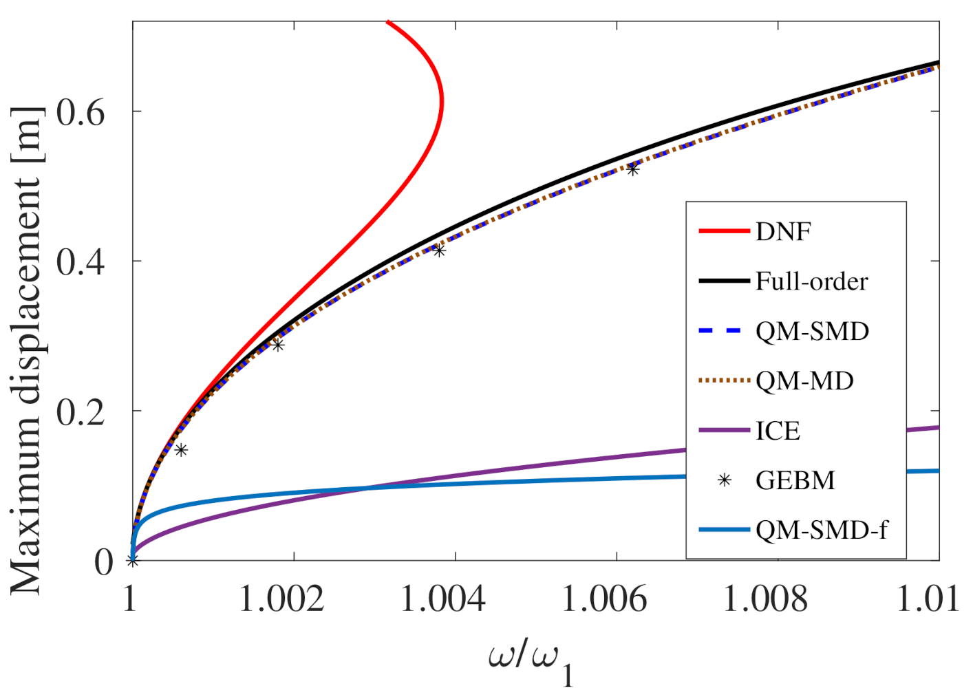
3.1. A Clamped–Clamped Beam with Increasing Curvature

The first example is a clamped–clamped beam, which is initially straight (case 1), for which two different levels of curvature are added to the neutral line in order to transform the beam into a shallow arch (case 2), and then into a non-shallow arch (case 3). Note that this example was first introduced in [50], where the comparison between the normal form result and the QM–MD and QM–SMD methods were compared on the backbone curves only. In this section, we extend these results by first adding the ICE method to the comparisons and, second, by considering a frequency-response function with damping and forcing. The geometries of the beams and the retained mesh are shown in Figure 3. The straight beam has a length of L = 0.7 m, and a square cross-section with equal thickness h and width b, h = b = 5 cm. The material is linear elastic (Young modulus E = 124 GPa, Poisson’s ratio ν = 0.3, and the density ρ = 4400 kg.m 3 ). The height of the static deflection of the shallow arch is 5.5 cm, while that of the non-shallow arch is 25 cm. Three-dimensional hexahedral finite elements with 20 nodes are used in each case. For the straight beam, 60 elements (four in the section and 15 in the length), resulting in a total number of 1287 dofs, were selected, while for the arches, a total of 96 solid elements (four in the section and 24 in the length), resulting in 2097 dofs, were used.
In each case, reduction to a single master mode is targeted by considering the nonlinear vibrations of the first bending mode. For the straight beam, the eigenfrequency of the first bending mode is f 1 = 545.60 Hz. For the shallow arch, the first bending appears as the second mode (by order of increasing frequency), with an eigenfrequency f 2 = 372.28 Hz, and for the non-shallow arch, it appears in the fourth position with f 4 = 1004 Hz. Let us first illustrate in this case how the ICE method is used to retrieve the nonlinear stiffness. Figure 4 shows the nonlinear relationship found by applying a static load of amplitude β on the first bending mode and its fitting by polynomial laws of orders 3, 5, and 7. A total of 100 values of applied loads were selected for the flat beam and the shallow arch cases, and 122 for the non-shallow arch. The load scales, as defined from the ICE method—see, e.g., [42,43,44,51]—were chosen to obtain displacements around the range of ±1.4 times the thickness for the beam case, 2 h to 3.8 h for the shallow arch, and 2.74 h to 1.56 h for the non-shallow arch. In each case, the application of the static force gives the displacement as a function of β , from which the fits allow one to invert the relationship. In particular, one can observe the appearance of strong even powers in the polynomial expansion for the last two cases with a non-symmetric restoring force. In these last two cases, the third-order approximation is not sufficient to correctly retrieve the stiffness behavior law, and an order of at least 5 is needed.
Figure 5 displays the backbone curves obtained for the three beams with increasing curvature. A reference solution was obtained via numerical continuation on all degrees of freedom by using a code with parallel implementation of the harmonic balance method and pseudo arc-length [68]. On the other hand, as the reduced dynamics were composed of a single master mode, the backbones were obtained numerically by continuation using a method combining harmonic balance and an asymptotic–numerical method implemented in Manlab [64,65,66].
In Figure 5a for the straight clamped–clamped beam, the slow/fast assumption is very well fulfilled and all methods easily catch the correct nonlinear behavior. The shallow arch results are shown in Figure 5b. In that case, the slow/fast assumption is just below the limit proposed in [50], since the ratio of eigenfrequencies between the first and the third bending modes is equal to 3.44. In addition, quadratic nonlinear couplings between bending modes appeared. For this main reason, the QM–SMD method fails to predict the correct nonlinear behavior of the backbone, as already remarked in [50]. The QM–MD and DNF reductions give almost equivalent results in terms of the backbone, which are close to the reference solution, but slightly depart when the amplitudes become large. Finally, in that case, the ICE method provides the best approximation to the reference solution, mostly because the fitting procedure is able to correctly retrieve the quadratic nonlinearity, and because the slow/fast assumption is not strongly violated. Note that for all of the figures, the ICE method was used in the reduction with the seventh-order fitted polynomial. Consequently, the order in the asymptotics is larger than in the other methods, which could also explain its better performance in that case.
In the case of the non-shallow arch, Figure 5c, the frequency ratio between third and first bending is 1.66, meaning that the slow/fast assumption is strongly broken. The consequence is that three methods are not able to retrieve the correct softening nonlinearity anymore: QM–MD and QM–SMD, as well as the ICE method, even though the ICE method is still pushed to the seventh order. In that case, the unfulfillment of the slow/fast assumption is stronger, so that whatever the order in the ICE method is, it will not converge to the correct value. On the other hand, the DNF method still predicts the correct nonlinear behavior and shows a slight departure at larger amplitudes, which is the only known limitation of the method and is linked to its asymptotic development.
A further insight is given into these results by computing the frequency-response functions (FRFs) for the three tested beams. In each case, a pointwise harmonic forcing is considered, located at the center of the beam, with an excitation frequency in the vicinity of the first bending mode. Rayleigh damping is added to the FE model, and a stiffness-proportional damping is taken into account such that the damping matrix reads C = b K . The value of the coefficient b was selected such that a damping ratio of 0.5% for the first bending mode was at hand, which leads to the following numerical values: b = 2.91 × 10 6 s for the straight beam, b = 4.27 × 10 6 s for the shallow arch, and b = 1.58 × 10 6 s for the non-shallow arch.
Figure 6 shows the obtained results when the four reduction methods are compared to the reference. Note that the treatment of the damping factor is strongly different in each case. The ICE method is the least efficient method for treating the damping. Indeed, by working on the fitting procedure of the nonlinear stiffness only, the method does not provide any means of including the damping of the slave modes in the reduced dynamics. Consequently, only the damping of the master mode is considered, which generally leads to a strong underestimation of the losses in the ROM. This is particularly true for the straight beam case in Figure 6a. On the other hand, for the two arches, the level of damping in the master mode is sufficient to approximately predict the correct maximum value in the FRF.
The other nonlinear reduction methods, QM and DNF, take the damping of the slave modes in the reduction process thanks to the nonlinear mapping. This leads to a perfect match with the reference solution in the beam case. For the arches, the problems already underlined in the backbone persist for the FRF. In particular, the QM–SMD method is not able to predict a correct FRF for the two arches, while the QM–MD method gives a correct computation for the shallow arch, but departs in the non-shallow arch case. The DNF method generally gives a correct approximation, but misses some slight quantitative information for the two arches, mainly due to the two approximations used to build the ROM: the asymptotics at the second order only and the treatment of the forcing, which are not strictly aligned with the nonlinear direction of the manifold, but simply with the linear eigenspace. The ICE method with an order of seven was used in each case, giving an excellent result in the shallow arch case, but it was generally expected to underestimate the losses, as observed in the beam and non-shallow arch cases.
As a conclusion of this example, one can observe that the ICE and QM methods need the fulfillment of the slow/fast assumption between the master and slave modes in order to predict the correct results. As already noted in [50], an incorrect treatment of the quadratic nonlinear terms in the QM–SMD method leads to problematic results once the second-order terms in the restoring force are important. The ICE method is able to rapidly propose an ROM with possibly higher orders, but fails as soon as the slow/fast assumption is violated. In addition, the method is not able to take into account the losses of the slave mode in the dynamics of the master mode. Finally, the DNF method always proposes the correct trend in terms of hardening/softening behavior, is able to properly take the damping of the slave modes into account, and is only limited to its fundamental assumptions linked to the asymptotics used and the treatment of the forcing.

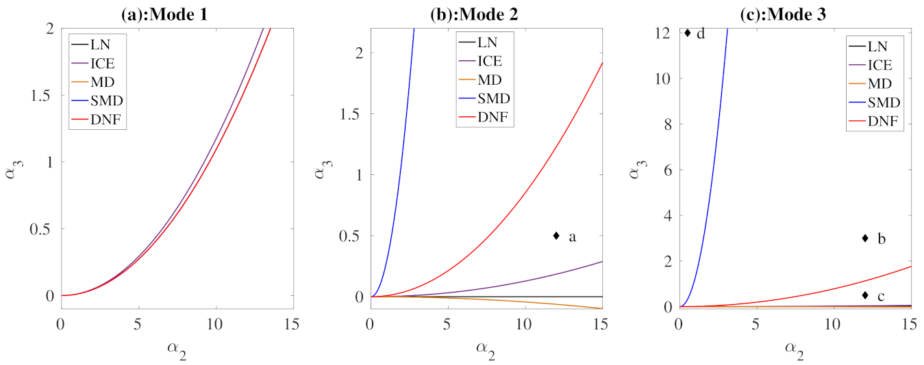
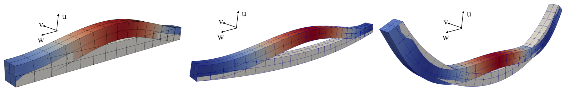
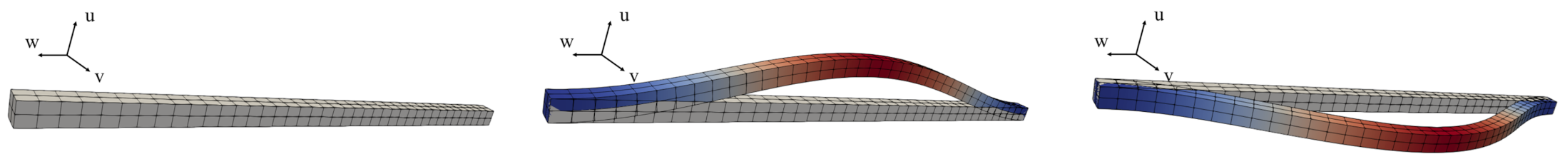
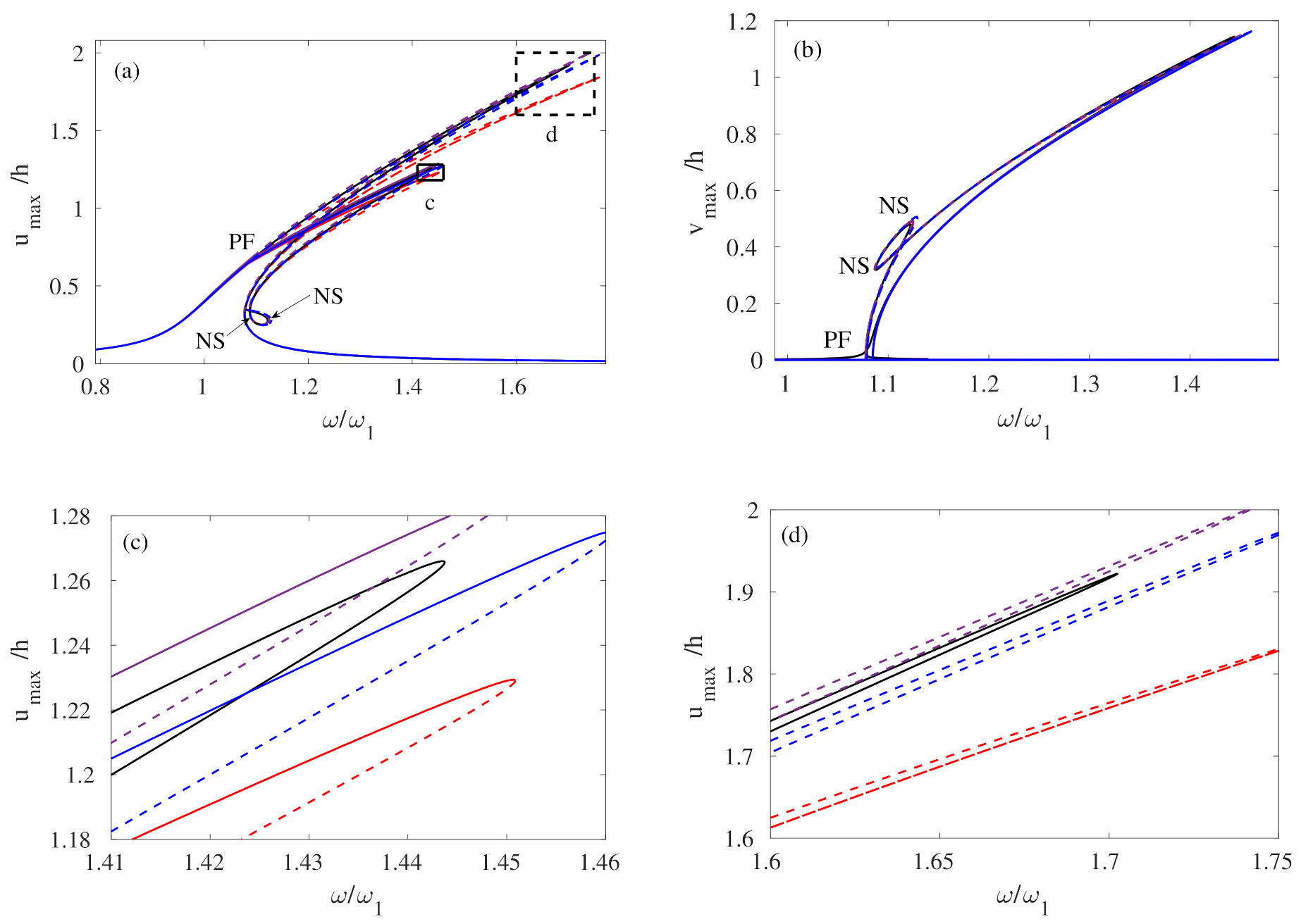
3.2. Clamped Beams with 1:1 Resonance

The second example is a straight clamped–clamped beam that is allowed to vibrate in the two bending directions, leading to different polarizations and, consequently, a 1:1 internal resonance. The objective of the comparison is to illustrate the ability of the methods to handle a more complex case with two master modes and bifurcations due to the presence of the internal resonance with the existence of coupled and uncoupled solutions [69,70].
Two different cases were investigated, where the constant parameters were: the length of the beam, 1 m, the density, ρ = 4400 kg/m 3 , the Young modulus, E = 1.04 × 10 11 Pa, and Poisson’s ratio, v = 0.3 . For the space discretization, 3D hexahedral brick elements with 20 nodes, and with 40 elements in the length and four in the cross-section, were used. The difference between the two beams is in their relative values of width b and thickness h. A first case with a perfect square section with h = b = 3 cm gives no detuning between the eigenfrequencies of the two polarizations of the first bending modes, which are perfectly equal. On the other hand, a second case with h = 3 cm and b = 3.15 cm allows the creation of a detuning of 4.92% between these two eigenfrequencies. Table 1 summarizes the geometrical parameters, and Figure 7 shows the retained mesh and the two polarizations of the fundamental bending mode (displacements along these two directions are denoted as u and v, and w is the in-plane motion).
Since the reduced dynamics contain two master coordinates, the fitting procedure for the ICE method first needs to create the two-dimensional stress manifold from which the nonlinear restoring force is deduced. The fitting procedure is illustrated in Figure 8. A total of 44 static load cases with different values of ( β 1 , β 2 ) are selected, where β i is the modal force amplitude factor applied on mode i. From these, the modal displacements ( X 1 , X 2 ) are retrieved from the static deformation, and a stress manifold is obtained, as shown in space ( X 1 , X 2 , β 1 ) in Figure 8. The load scales are chosen so as to obtain amplitudes of displacements in the range of ±1 times the thickness. The perfect and detuned cases are considered, and they show a clear symmetric stress manifold.

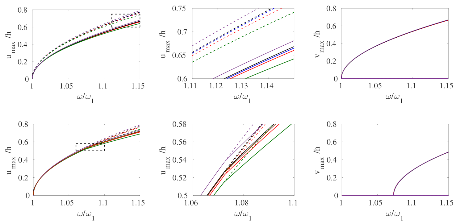
3.2.1. Backbone Curves

We first report the computation of the backbone curves in the two selected cases with and without detuning. As in the previous section, a reference solution was derived thanks to numerical continuation on the full-order model, and was compared to the ROMs with two master coordinates. The analytical solution derived in [70] allows a better understanding of the expected results. In particular, when detuning is present, an uncoupled solution in which only the lowest frequency mode is excited exists until a pitchfork bifurcation point, where this solution becomes unstable in favor of a coupled solution corresponding to an elliptic mode.
Figure 9 shows the obtained results. The first row corresponds to the case without detuning, while the second row corresponds to the case with detuning. In order to correctly represent the two vibration polarizations, the displacements at the center of the beam in the two u and v directions (see Figure 7) are reported. When there is no detuning, two types of backbone curves are numerically retrieved: an unstable solution, corresponding to an uncoupled mode where only the displacement along u is excited (such that v = 0 ), and a stable coupled solution with both u 0 and v 0 . With the detuning, the coupled solution branches from the uncoupled one at a pitchfork bifurcation point. The main conclusion is that all of the methods are able to correctly retrieve the unforced and undamped dynamics of this problem, with all the specific analytical features in terms of existence, stability, and bifurcations of the 1:1 internally resonant dynamics. This is easily explained by looking at the reduced dynamics computed by each of the methods, which are reported in Appendix B. As a matter of fact, the dynamical equations contain only the four resonant monomial terms that are also retained in the analytical developments provided in [70]. All of the other terms are negligible. The slow/fast assumption is very well fulfilled, and no quadratic terms are present. Consequently, all of the methods are able to retrieve such dynamics, which are fully driven by only four cubic terms, without invariant-breaking terms.

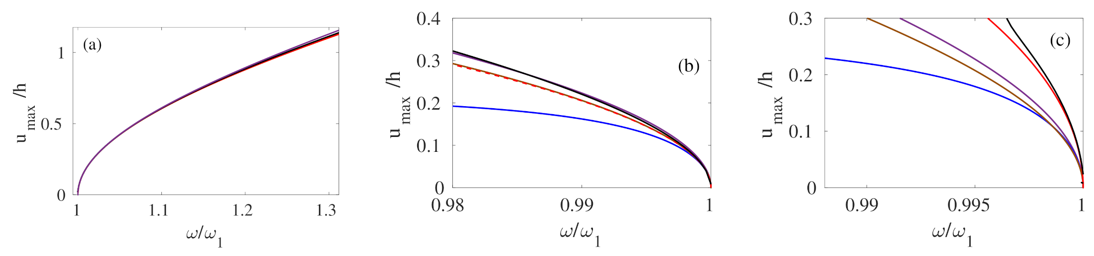
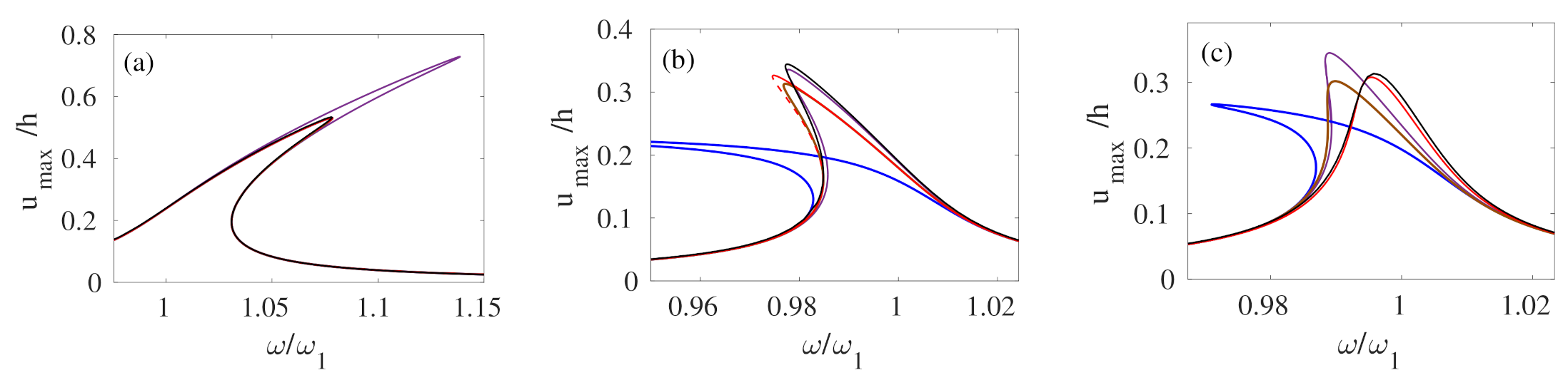
3.2.2. Frequency-Response Curves

The forced–damped dynamics are now investigated by computing the FRFs. A forcing term aligned with direction u is imposed at the center of the beam in order to excite one polarization and to observe the nonlinear coupling with the second polarization along v. A Rayleigh damping of the form C = b K is selected, with b = 1.0622 × 10 5 s , corresponding to a damping ratio of 0.5 percent for the first mode. The reduction methods are compared to the full-order reference solution, all of them being obtained by numerical continuation. Note, however, that the continuation method implemented in [68] is not yet able to perform the stability computation or to locate pitchfork bifurcation points. In order to circumvent the second limitation, a small forcing in the v direction, with an amplitude selected as 1 % of the amplitude in the u direction, is also applied. Consequently, the solution is perturbed with a non-zero solution in the v direction, allowing the continuation method to retrieve the coupled branch. On the other hand, the FRFs of the reduced dynamics are computed with Manlab [64,65,66], which reports stability and detects pitchfork bifurcations.
Let us first illustrate the results found in the case without detuning, shown in Figure 10, where the amplitude of the forcing is set to 300 N. The topology of the solution, which was already reported in other cases (see, e.g., [28]), is characterized by a pitchfork bifurcation point from which the branch of coupled solutions arise. Along this solution branch, two Neimark–Sacker bifurcation points exist, leading to quasi-periodic solutions in this area. Importantly, all of the methods are able to retrieve all of these important dynamical features. Small quantitative differences are observable. The ICE method strongly underestimates the damping in the reduced dynamics. This is, again, a consequence of the treatment of the losses by the reduction method, which is not able to take into account the damping factors of the slave modes. On the other hand, the QM and DNF methods produce a very satisfactory prediction of the full dynamics. The QM–MD and QM–SMD methods give completely equivalent results in this case; the curves fully overlap. Indeed, as reported in Appendix B, in this particular case, using either MDs or SMDs in the reduction method for building the quadratic manifold produces exactly the same equations for the reduced dynamics. Consequently, in this section, only the results of the QM–SMD method are shown in the figures. A slightly better quantitative prediction is given by the DNF method on the second polarization (companion mode); in any case, this difference is small. One can also remark that the trick used to get the coupled solution for the full-order model is visible close to the imperfect pitchfork bifurcation points for the second polarization.
The results for the beam with detuning ε = 4.92 % are shown in Figure 11, where the Rayleigh damping is now mass-proportional and has been set to C = a M with a = 9.4147 s 1 (still following the rule of 0.5 percent for the first mode), and the amplitude of the forcing is 1500 N, a large value that is needed in order to correctly enter the coupled branch solution, reaching vibration amplitudes close to two times the thickness. One can note that, in this case, all of methods give very close results. In particular, using mass-proportional damping creates damping ratios that decrease with increasing frequencies. Consequently, the damping values of the slave modes are smaller and smaller. The consequence is that most of the losses are given by the modal damping factor of the master modes, so that the ICE method is now able to give a correct prediction as compared to the other methods. The QM–MD and QM–SMD methods again perfectly overlap for the same reason as before; consequently, only the QM–SMD curve is shown. The branch of coupled solutions arises from in a pitchfork bifurcation, and two Neimark–Sacker bifurcation points exist along this branch, leading to quasi-periodic solutions. Once again, these dynamical features can be retrieved by all of the methods.
As a conclusion of this case, one can observe that all of the methods are able to reproduce the 1:1 internally resonant dynamics well by taking two master modes into account. The main reason resides in the fact that the reduced dynamics are only driven by four resonant monomial terms that are easy to retrieve, regardless of the method used. In addition, the slow/fast assumption is very well verified, so the ICE and QM methods can predict the correct results. All of these conclusions should be different in the case of a shell with 1:1 internal resonance, since in this case, the slow/fast assumption and the appearance of strong quadratic couplings would completely change the picture. A preliminary result in this direction is reported in [60], where it is observed that for a spherical-cap shell, the QM method is not able to retrieve the correct type of nonlinearity due to the violation of the slow/fast assumption.

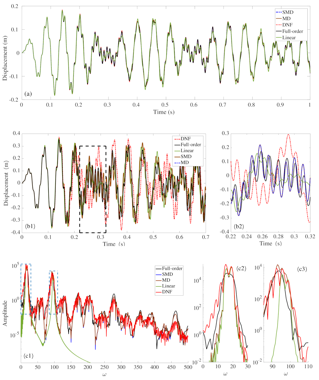
3.3. A Cantilever Beam

The last of the investigated examples is a cantilever beam with length L = 1 m and a cross-section with width b = 0.05 m and thickness h = 0.02 m. The material parameters used are the density, ρ = 4400 kg/m 3 , the elastic modulus, E = 1.04 × 10 11 Pa, and Poisson’s ratio, ν = 0.3 . The beam is discretized with a 3D hexahedral element with 20 nodes. A total of 50 elements in the length and four elements in the cross-section are used. For this last example, the backbone curve of the fundamental mode is under study, together with time-domain simulations with multi-frequency forcings, in order to test the ability of the ROMs to retrieve the correct type of nonlinearity and their accuracy with more than one master mode in the reduction basis. The first five radian eigenfrequencies of the cantilever beam are ω 1 = 99.00 (rad/s), ω 2 = 246.79 (rad/s), ω 3 = 619.31 (rad/s), ω 4 = 1529.1 (rad/s), and ω 5 = 1729.3 (rad/s), showing no obvious internal resonance relationships among them.
Let us first illustrate the computation of the backbone curve of the fundamental bending mode. The ICE procedure is illustrated in Figure 12 using a single master coordinate. A total of 100 values of applied load cases were selected to obtain displacements at the tip of the cantilever in the range of ± 0.47 m, meaning that very large displacements of up to almost one-half the length were considered. One can observe that the fitting with the third order is not accurate enough, indicating the need for a higher order. In the remainder of the computations, the ROM obtained with the ICE method is considered up to order seven.
Figure 13 shows the backbone curves. Apart from the classical analytical model initially proposed in [71] and asymptotically truncated to the third order, for which the backbone curves of the first bending modes were computed, for instance, in [72,73], very few numerical attempts to accurately compute those backbone curves for very large amplitudes have been proposed. The only reference is [74], which is based on a geometrically exact beam model (GEBM). Figure 13 reports those results with black stars, which are labeled as GEBM. Each point corresponds to the time integration of the beam model, discretized with 20 Timoshenko first-order finite elements, under harmonic driving in the steady state at the nonlinear resonance (the point at which the amplitude is maximal), which is very close to the phase resonance corresponding to the backbone curve (see [74] for details about the geometrically exact beam model and [75] for the phase resonance). This reference solution attests to a slight hardening behavior up to very large amplitudes that are equivalent to more than half the length of the beam. The results of this beam model are very close to the reference full-order solution that was obtained with the present 3D finite element model of the beam; the slight difference is attributed to the differences between the models (3D and beam model).
Comparing the ROMs, the ICE method gives the most incorrect result, with a strong overprediction of the hardening behavior. As the method is essentially static, it is known that it faces important failures when an inertia nonlinearity is present. The DNF method gives the correct behavior up to a vibration amplitude of approximately 0.2 m, meaning that the method is reliable up to 1/5 of the beam’s length. Then, the solution strongly departs from the reference. This limitation is due to the third-order dynamics of the reduction method, and taking higher orders into account would improve the result.
The QM methods—using either MDs or SMDs—give identical reduced dynamics again in this case. Importantly, they offer the best solution for this specific case, with vibration amplitudes of up to more than 0.6 times the length of the beam. One can note that the result presented here is different from the one reported in [46], where the QM–SMD method was found to fail in a similar cantilever case. In order to understand this discrepancy, another implementation of the QM-SMD method was applied to the same case, and is referred to as “QM-SMD-f” case (where the added letter -f refers to “full” QM SMD approach). In this version, the reduced dynamics used to compute the backbone curve are the untruncated ones given by Equation (14), with polynomial terms up to order seven, which are the ones used in [46] and are different from the ones we used throughout this paper, where all reduced dynamics given by the QM method have been truncated to the third order. Interestingly, the full implementation of the QM–SMD method gives very incorrect results, following the conclusions drawn in [46]. On the other hand, our implementation of the QM method with dynamics truncated up to order three gives an excellent result, underlining that unbalanced higher-order terms have a huge effect on the prediction of the reduced dynamics in this specific case.
In order to further illustrate the comparison, time responses were computed with harmonic forcings with two and three driving frequencies that were located at the free tip of the cantilever in order to test the ability of the different methods with either two or three master modes. In this last comparison, only the QM-based methods and the DNF method were studied. Indeed, as already reported in [44,51], the fitting procedure with an increasing number of master modes in the ICE method becomes more and more difficult and subject to important variations depending on the load scales selected. Second, the computations reported in [76] underline the limits of the ICE method for tackling a problem including inertia nonlinearity, such as in the present case of a cantilever beam. Finally, the incorrect results found with only one master mode, as well as preliminary computations with two master modes, clearly underline that the ICE method gives results that are too far from the reference. Therefore, the results of the ICE method will no longer be shown in this case.
For the numerical time integration, a Newmark- β scheme with β = 0.25 and γ = 0.5 was selected. The time step of τ = 0.0001 s corresponds to a sampling rate of 10 kHz with 20 points per period, ensuring accuracy up to mode 6. In addition, this value is large compared to the selected forcing frequency, and thus excites the low-frequency modes in the range of [ 15 , 300 ] Hz. A mass-proportional Rayleigh damping with C f = 2 [ M ] (in s 1 ) is taken into account, corresponding to a damping ratio of 1% for the first mode. In each case, the initial conditions correspond to the structure at rest.
The first case considers a two-frequency harmonic excitation, with driving frequencies in the vicinity of the first and third eigenfrequencies of the structure. More precisely, the temporal content of the external force reads f ( t ) = F 0 ( sin ( 1.21 ω 1 t ) + sin ( 0.97 ω 3 t ) ) , and two different amplitudes of the forcing are tested, F 0 = 400 N and F 0 = 800 N, in order to reach vibration amplitudes of up to 0.2 m (1/5 of the length of the cantilever) and 0.4 m, respectively. Figure 14 shows the obtained results, where the full-order solution assuming a linear restoring force is also shown in green. Neglecting the nonlinear terms in Equation (1) allows a direct assessment of the level of excited nonlinearity. In Figure 14a with F 0 = 400 N, the level of nonlinearity is too small and all vibrations’ data are very close to each other for the reduced models as well as for the linear assumption. This is not the case anymore for F 0 = 800 N, and Figure 14b,c show both the temporal and frequency content. The importance of the nonlinearities is particularly well assessed in Figure 14c, where one can observe that the linearized system is not able to reproduce the important frequency content outside the excitation frequencies. Now, comparing the reduction methods, the QM–MD and QM–SMD methods offer the best comparison to the full-order reference solution, with time traces and spectra that are very close. On the other hand, the DNF method slightly departs from the reference solution. This is again attributed to the second-order truncation used in the present DNF approach, and higher orders should be able to recover better results. However, one can note that the correct predictive behavior of the DNF method fails to accurately reproduce details in the time trace, but remains very close to the reference in terms of frequency content, meaning that only slight phase problems are present.
The gains in using ROMs for time integration are very important. The full-order analysis was run using Code_Aster for approximately 24 h on a 12-core processor computer with 16 GB of RAM and a CPU at 2.20GHz, and the construction and utilization of the reduced-order models only took about 3 min for the same simulation.
The last case under study is an excitation with three driving frequencies, temporal content selected as f ( t ) = sin ( 1.21 ω 1 t ) + sin ( 0.97 ω 3 t ) + sin ( 0.98 ω 5 t ) , and an amplitude of 400 N. The ROMs were built with three master coordinates corresponding to modes 1, 3, and 5. Figure 15 shows the results obtained in both the time and frequency domains. In this case, the nonlinearity is sufficiently excited with a forcing amplitude of 400 N, and very important differences already appear between time traces and frequency content. Regarding the ROMs, one can observe that the QM-based methods give excellent results that are almost coincident with those of the full-order model. On the other hand, the DNF method shows a slight departure from the reference solution. One can note, however, that this departure is moderate, with small shifts in the time domain, but a very good recovery of the frequency content. The full-order analysis was run using Code_Aster for approximately 20 h on the same computer mentioned above; the construction and utilization of the reduced-order models still only took about three minutes.
To conclude this example, the three reduction methods (ICE, QM, and DNF) were tested on a cantilever beam. The ICE method was not able to successfully handle this case, mainly due to the importance of the nonlinear inertia effects that are missed in the construction of the ROM. The DNF method gave good results up to an amplitude of 1/5 of the length of the cantilever, in line with the results reported in [48] on a clamped–free fan blade. One advantage of the method is that it always predicts the correct hardening/softening behavior at the first order, and it relies on invariant manifold theory. On the other hand, when reaching very large amplitudes, the limitation of using third-order asymptotics comes into play. The QM methods gave excellent results in this case when used with either full or static modal derivatives. This is in contrast with the results of [46], where an untruncated version of the reduced dynamics was used for that case, such that the higher-order terms introduced in the dynamics by the quadratic part were not balanced by higher-order terms in the nonlinear mapping. On the other hand, our computations show that, when limited to the third order, the QM methods give excellent predictions in the cantilever case. This result would need further investigation in order to offer a complete understanding. Indeed, at present, there are no theoretical arguments supporting a better behavior of the QM method. As demonstrated in [50], the QM methods do not project the problem on an invariant manifold and need the slow/fast assumption to retrieve the correct results. Even though the slow/fast separation is well fulfilled in this case, there is no explanation that the methods could provide such perfect predictions up to very large amplitudes. One reason might come from the acceleration terms that are produced by the method in the reduced dynamics.

4. Conclusions

In this contribution, three nonlinear reduction methods for thin beam structures vibrating with large amplitudes were compared: the implicit condensation and expansion (ICE) method, the quadratic manifold (QM) methods using either full modal derivatives (MDs) or only static modal derivatives (SMDs), and the direct normal form (DNF) method. From the theoretical point of view, the three methods propose a reduction of a curved subspace, a feature that is needed to take the nonlinear couplings into account. Only the last two propose a nonlinear mapping to go from the physical space to the reduction space, and only the DNF method relies on invariant manifolds, which is a key feature in order to produce accurate and reliable ROMs. Indeed, when the reduction subspaces are not invariant, the trajectories produced by the ROM do not correspond to any trajectory of the full system, which might be problematic. An important consequence shown in [49,50,51] is that the ICE and QM-based methods need a slow/fast separation between the master and slave coordinates in order to predict the correct results.
The methods were first compared on an academic, analytical example, a linear beam resting on a nonlinear elastic foundation, with the main aim of underlining how the ICE and QM methods can fail in their predictions due to the fact that the slow/fast assumption is not fulfilled. A feature also underlined in [50] is the incorrect treatment of the quadratic nonlinearity by the QM–SMD method, leading to unreliable results when the quadratic terms dominate.
Then, FE-based beam examples were selected in order to offer a more complete picture of the advantages and drawbacks of the methods. In the first example, the curvature was added to a straight clamped–clamped beam, enforcing important nonlinear quadratic couplings together with an unfulfillment of the slow/fast assumption. Similar conclusions to those from the academic, analytical example were drawn. A straight beam with two polarizations was then studied, showing that all of the tested methods were able to correctly retrieve these 1:1 internally resonant dynamics. Finally, a cantilever beam was investigated, showing that ICE method could not catch the correct behavior from the small amplitudes, whereas the DNF method allowed correct prediction of up to 1/5 of the length of the beam, and the QM methods gave excellent results up to larger amplitudes, more than 1/2 of the length for the backbone of the fundamental mode. It has been underlined that these results need further investigation, as they are different from the results reported in [46], and there is no theoretical support yet that can explain such good results.
As a summary of the different methods, one can underline the following results. For the ICE method, the main advantage resides in its ease of use and in the rapid and correct results it might give when only one master mode is considered and the slow/fast assumption is verified. On the other hand, it is not reliable when the S/F assumption is not valid anymore, and as it is a static method in essence, it encounters strong difficulties in a case such as the cantilever beam. Finally, the treatment of the damping is elementary, and the loss factors of the slave modes are not taken into account in the reduced dynamics, generally leading to underprediction of the losses in the reduced dynamics.
The QM methods also need the slow/fast assumption and fail in predicting the correct type of nonlinearity when it is not fulfilled. The QM–SMD method proposes a treatment of the quadratic nonlinearity that can lead to erroneous predictions. On the other hand, the QM-MD method generally gives better results. The QM methods propose an improvement as compared to the ICE method, as shown in the numerous examples derived in this article. In particular, the treatment of the damping is more robust and takes the slave modes into account. Further insight is needed in the case of the cantilever to better understand the behavior of the reduction method.
The DNF method has the invariance property embedded and generally includes the most appealing theoretical features without needing any extra assumptions for its use. It is limited to its third-order asymptotics, so the results are expected to deteriorate at very large amplitudes, which was clearly observed in the cantilever beam example. It offers a general treatment of damping that includes the slave modes. Other limitations are linked to the assumption made to take into account the forcing, which might need further developments.
All of the results presented in this paper are limited to beam examples. Further studies should enlarge the scope to include more complex structures and, more specifically, the case of shells, where the differences between the methods should be more pronounced.

Author Contributions

Writing—original draft preparation: Y.S. and C.T.; writing—review and editing: all authors; conceptualization and methodology: A.V., L.S., O.T., and C.T.; computational developments: Y.S., A.V., T.Y., and L.S.; formal analysis: A.V. and C.T.; numerical investigation: Y.S. and N.K.; supervision: L.S., O.T., and C.T. All authors have read and agreed to the published version of the manuscript.

Funding

Y. Shen wishes to thank the China Scholarship Council (No. 201806230253) for the funding of a three-year doctoral position at IMSIA, ENSTA Paris, and EDF Lab. A. Vizzaccaro is thankful to Rolls-Royce plc for the financial support. L. Salles is thankful to Rolls-Royce plc and the EPSRC for their support under the Prosperity Partnership Grant ”Cornerstone: Mechanical Engineering Science to Enable Aero-Propulsion Futures”, Grant Ref: EP/R004951/1.

Informed Consent Statement

Not applicable.

Data Availability Statement

Not applicable.

Acknowledgments

The authors are thankful to Attilio Frangi (Politecnico di Milano) for discussions on the reduction methods and Jiri Blahos for the development of the numerical continuation method for full-order solutions.

Conflicts of Interest

The authors declare no conflict of interest.

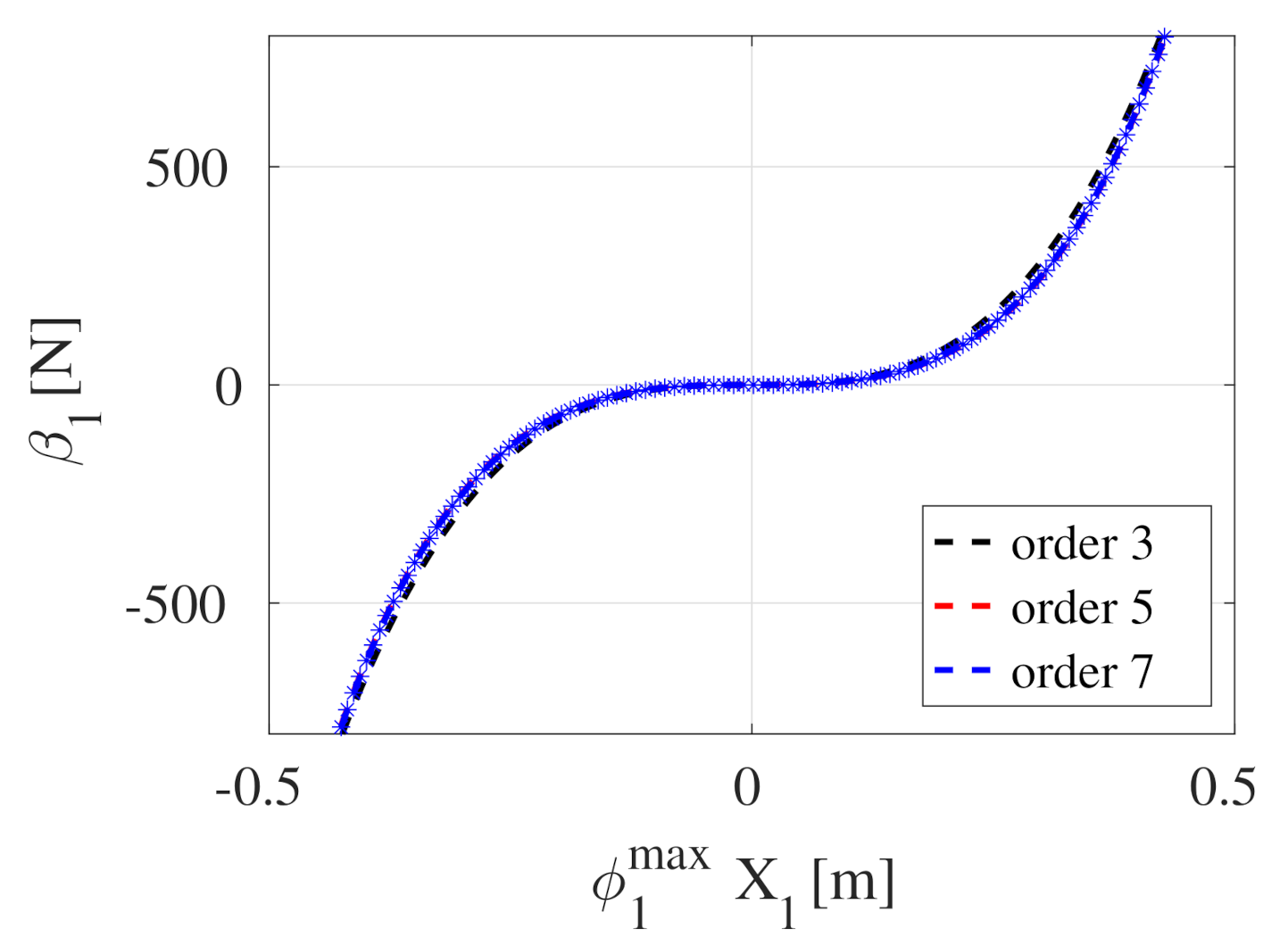
Appendix A. Representation of Quadratic and Cubic Nonlinear Terms

In this appendix, detailed expressions of the quadratic and cubic polynomial terms representing the nonlinear internal restoring force are provided for clarity. The equations of motion in physical coordinates are given by Equations (1) and (2), where the internal force vector reads F ( u ) = K u + G ( u , u ) + H ( u , u , u ) . Explicit expressions of G ( u , u ) and H ( u , u , u ) are written as:
G ( u , u ) = r = 1 N s = 1 N G r s u r u s ,
H ( u , u , u ) = r = 1 N s = 1 N t = 1 N H r s t u r u s u t ,
where G r s and H r s t are the N-dimensional vectors of coefficients G r s p and H r s t p for p = 1 , , N . Using the matrix of eigenvectors, this problem can be rewritten on the modal basis as in Equation (4), using similar notations for the quadratic and cubic tensors of coefficients. The k-th modal equation thus reads:
X ¨ k + 2 ζ k ω k X ˙ k + ω k 2 X k + i = 1 N j = i N g i j k X i X j + i = 1 N j = i N l = j N h i j l k X i X j X l = Q k ,
and the relationships between G and g and H and h read:
g i j = P ϕ T G ( ϕ i , ϕ j ) ,
h i j k = P ϕ H ( ϕ i , ϕ j , ϕ k ) .

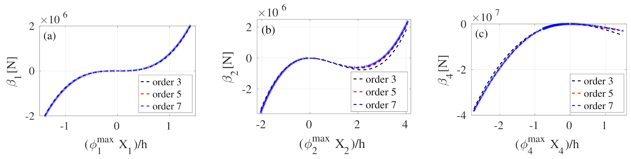
Appendix B. Reduced Dynamics for the Clamped Beam with 1:1 Resonance

In this appendix, the explicit equations used for the reduced-order dynamics of the clamped–clamped beam with 1:1 internal resonance between the two polarizations are given in order to offer a better understanding of the simulated dynamics. The equations are given only in the case without detuning and for the undamped–unforced case.
Using the ICE method, the polynomial third-order fitting from the set of imposed forcings allows one to retrieve the following reduced dynamics:
R 1 ¨ + 8.8618 e 5 R 1 + 4.3527 e 8 R 1 3 + 4.5018 e 8 R 1 R 2 2 = 0 ,
R 2 ¨ + 8.8624 e 5 R 2 + 4.3575 e 8 R 2 3 + 4.4893 e 8 R 2 2 R 1 = 0 .
Note that, in the fitting procedure, only the nonlinear terms are assessed. The linear ones are given as known from the eigenanalysis. The small difference between the two squared eigenfrequencies is the consequence of the small difference in the computed eigenfrequencies reported in Table 1, which is due to numerical roundoff. Only four monomial terms are needed, and they correspond to the ones studied in [70].
The ROM computed with the DNF method reads:
R 1 ¨ + 8.8618 e 5 R 1 + 4.5659 e 8 R 1 3 + 4.5657 e 8 R 1 R 2 2 + 0.1265 R 1 R ˙ 1 2 + 0.0042 R 2 R ˙ 1 R ˙ 2 + 0.1224 R 1 R ˙ 2 2 = 0 ,
R 2 ¨ + 8.8624 e 5 R 2 + 4.5657 e 8 R 1 2 R 2 + 4.5659 e 8 R 2 3 + 0.1265 R 2 R ˙ 2 2 + 0.0042 R 1 R ˙ 1 R ˙ 2 + 0.1224 R 2 R ˙ 1 2 = 0 .
The linear part is left unchanged (identity-tangent nonlinear mapping). One can observe that the additional monomials (involving squared velocities) are obviously negligible as compared to the four resonant cubic terms already present in Equation (A5). This clearly underlines that the dynamics are completely driven by the most simple system, with only four resonant monomial terms corresponding to 1:1 internal resonance.
Using the QM–SMD method, a different nonlinear mapping is introduced. As already observed in [50], the QM–SMD method produces many more monomial terms in the reduced dynamics, with additional terms involving the accelerations. The reduced dynamics now read:
R 1 ¨ + 8.8618 e 5 R 1 + 4.5670 e 8 R 1 3 + 4.5668 e 8 R 1 R 2 2 + 0.1263 R 1 2 R ¨ 1 + 0.1243 R 1 R 2 R ¨ 2 + 0.0021 R 2 2 R ¨ 1 + 0.1263 R ˙ 1 2 R 1 + 0.1243 R ˙ 1 R ˙ 2 R 2 + 0.0021 R ˙ 2 2 R 1 = 0 ,
R 2 ¨ + 8.8624 e 5 R 2 + 4.5670 e 8 R 2 3 + 4.5668 e 8 R 2 2 R 1 + 0.1263 R 2 2 R ¨ 2 + 0.1243 R 2 R 1 R ¨ 1 + 0.0021 R 1 2 R ¨ 2 + 0.1263 R ˙ 2 2 R 2 + 0.1243 R ˙ 2 R ˙ 1 R 1 + 0.0021 R ˙ 1 2 R 2 = 0 .
Again, one can observe that in this particularly simple case of a straight beam, all of the added terms have negligible coefficients. Again, the dynamics are driven by the simple system composed of only four cubic terms. The same is also observed when applying the QM–MD method, leading to the following reduced dynamics:
R 1 ¨ + 8.8618 e 5 R 1 + 4.5670 e 8 R 1 3 + 4.5668 e 8 R 1 R 2 2 + 0.1264 R 1 2 R ¨ 1 + 0.1243 R 1 R 2 R ¨ 2 + 0.0021 R 2 2 R ¨ 1 + 0.1264 R ˙ 1 2 R 1 + 0.1243 R ˙ 1 R ˙ 2 R 2 + 0.0021 R ˙ 2 2 R 1 = 0 ,
R 2 ¨ + 8.8624 e 5 R 2 + 4.5670 e 8 R 2 3 + 4.5668 e 8 R 2 2 R 1 + 0.1264 R 2 2 R ¨ 2 + 0.1243 R 2 R 1 R ¨ 1 + 0.0021 R 1 2 R ¨ 2 + 0.1264 R ˙ 2 2 R 2 + 0.1243 R ˙ 2 R ˙ 1 R 1 + 0.0021 R ˙ 1 2 R 2 = 0 .
In this particular case, the reduced dynamics given by QM–SMD and QM–MD are completely equivalent, explaining that the methods produce exactly the same predictions. Note, however, that this result is specific to the studied case, and more complex structures generally lead to different formulations for the MD and SMD approaches.

References

  1. Steindl, A.; Troger, H. Methods for dimension reduction and their applications in nonlinear dynamics. Int. J. Solids Struct. 2001, 38, 2131–2147. [Google Scholar] [CrossRef]
  2. Rega, G.; Troger, H. Dimension reduction of dynamical systems: Methods, models, applications. Nonlinear Dyn. 2005, 41, 1–15. [Google Scholar] [CrossRef]
  3. Nayfeh, A.H.; Mook, D.T. Nonlinear Oscillations; John Wiley & Sons: New York, NY, USA, 1979. [Google Scholar]
  4. Amabili, M. Nonlinear Vibrations and Stability of Shells and Plates; Cambridge University Press: Cambridge, UK, 2008. [Google Scholar]
  5. Awrejcewicz, J.; Krysko, V.A.; Narkaitis, G. Bifurcations of a Thin Plate-Strip Excited Transversally and Axially. Nonlinear Dyn. 2003, 32, 187–209. [Google Scholar] [CrossRef]
  6. Nayfeh, A.H.; Balachandran, B. Modal interactions in dynamical and structural systems. ASME Appl. Mech. Rev. 1989, 42, 175–201. [Google Scholar] [CrossRef]
  7. Nayfeh, A.H. Nonlinear Interactions: Analytical, Computational and Experimental Methods; Wiley Series in Nonlinear Science; John Wiley & Sons: Hoboken, NJ, USA, 2000. [Google Scholar]
  8. Thomas, O.; Touzé, C.; Luminais, E. Non-linear vibrations of free-edge thin spherical shells: Experiments on a 1:1:2 internal resonance. Nonlinear Dyn. 2007, 49, 259–284. [Google Scholar] [CrossRef] [Green Version]
  9. Monteil, M.; Touzé, C.; Thomas, O.; Benacchio, S. Nonlinear forced vibrations of thin structures with tuned eigenfrequencies: The cases of 1:2:4 and 1:2:2 internal resonances. Nonlinear Dyn. 2014, 75, 175–200. [Google Scholar] [CrossRef] [Green Version]
  10. Vizzaccaro, A.; Givois, A.; Longobardi, P.; Shen, Y.; Deü, J.F.; Salles, L.; Touzé, C.; Thomas, O. Non-intrusive reduced order modelling for the dynamics of geometrically nonlinear flat structures using three-dimensional finite elements. Comput. Mech. 2020. accepted for publication. [Google Scholar] [CrossRef]
  11. Awrejcewicz, J.; Krysko, V.A.; Saveleva, N. Routes to chaos exhibited by closed flexible cylindrical shells. ASME J. Comput. Nonlinear Dyn. 2007, 2, 1–9. [Google Scholar] [CrossRef]
  12. Touzé, C.; Thomas, O.; Amabili, M. Transition to chaotic vibrations for harmonically forced perfect and imperfect circular plates. Int. J. Non-Linear Mech. 2011, 46, 234–246. [Google Scholar] [CrossRef] [Green Version]
  13. Cadot, O.; Ducceschi, M.; Humbert, T.; Miquel, B.; Mordant, N.; Josserand, C.; Touzé, C. Wave turbulence in vibrating plates. In Handbook of Applications of Chaos Theory; Skiadas, C., Ed.; Chapman and Hall/CRC: Boca Raton, FL, USA, 2016. [Google Scholar]
  14. Kapania, R.K.; Byun, C. Reduction methods based on eigenvectors and Ritz vectors for nonlinear transient analysis. Comput. Mech. 1993, 11, 65–82. [Google Scholar] [CrossRef]
  15. Krysl, P.; Lall, S.; Marsden, J. Dimensional model reduction in non-linear finite element dynamics of solids and structures. Int. J. Numer. Methods Eng. 2001, 51, 479–504. [Google Scholar] [CrossRef]
  16. Kerschen, G.; Golinval, J. Physical interpretation of the proper orthogonal modes using the singular value decomposition. J. Sound Vib. 2002, 249, 849–865. [Google Scholar] [CrossRef] [Green Version]
  17. Sampaio, R.; Soize, C. Remarks on the efficiency of POD for model reduction in non-linear dynamics of continuous elastic systems. Int. J. Numer. Methods Eng. 2007, 72, 22–45. [Google Scholar] [CrossRef] [Green Version]
  18. Amabili, M.; Sarkar, A.; Païdoussis, M.P. Chaotic vibrations of circular cylindrical shells: Galerkin versus reduced-order models via the proper orthogonal decomposition method. J. Sound Vib. 2006, 290, 736–762. [Google Scholar] [CrossRef]
  19. Amabili, M.; Touzé, C. Reduced-order models for non-linear vibrations of fluid-filled circular cylindrical shells: Comparison of POD and asymptotic non-linear normal modes methods. J. Fluids Struct. 2007, 23, 885–903. [Google Scholar] [CrossRef] [Green Version]
  20. Shaw, S.W.; Pierre, C. Non-linear normal modes and invariant manifolds. J. Sound Vib. 1991, 150, 170–173. [Google Scholar] [CrossRef] [Green Version]
  21. Shaw, S.W.; Pierre, C. Normal modes for non-linear vibratory systems. J. Sound Vib. 1993, 164, 85–124. [Google Scholar] [CrossRef] [Green Version]
  22. Carr, J. Applications of Centre Manifold Theory; Springer: New York, NY, USA, 1981. [Google Scholar]
  23. Guckenheimer, J.; Holmes, P. Nonlinear Oscillations, Dynamical Systems and Bifurcations of Vector Fields; Springer: New York, NY, USA, 1983. [Google Scholar]
  24. Pesheck, E.; Boivin, N.; Pierre, C.; Shaw, S.W. Nonlinear Modal Analysis of Structural Systems Using Multi-Mode Invariant Manifolds. Nonlinear Dyn. 2001, 25, 183–205. [Google Scholar] [CrossRef]
  25. Jiang, D.; Pierre, C.; Shaw, S. Nonlinear normal modes for vibratory systems under harmonic excitation. J. Sound Vib. 2005, 288, 791–812. [Google Scholar] [CrossRef]
  26. Apiwattanalunggarn, P.; Pierre, C.; Jiang, D. Finite-Element-based nonlinear modal reduction of a rotating beam with large-amplitude motion. J. Vib. Control 2003, 9, 235–263. [Google Scholar] [CrossRef]
  27. Touzé, C.; Thomas, O.; Chaigne, A. Hardening/softening behaviour in non-linear oscillations of structural systems using non-linear normal modes. J. Sound Vib. 2004, 273, 77–101. [Google Scholar] [CrossRef] [Green Version]
  28. Touzé, C.; Amabili, M. Non-linear normal modes for damped geometrically non-linear systems: Application to reduced-order modeling of harmonically forced structures. J. Sound Vib. 2006, 298, 958–981. [Google Scholar] [CrossRef] [Green Version]
  29. Touzé, C. Normal form theory and nonlinear normal modes: Theoretical settings and applications. In Modal Analysis of Nonlinear Mechanical Systems; Kerschen, G., Ed.; Springer Series CISM Courses and Lectures; Springer: New York, NY, USA, 2014; Volume 555, pp. 75–160. [Google Scholar]
  30. Touzé, C.; Amabili, M.; Thomas, O. Reduced-order models for large-amplitude vibrations of shells including in-plane inertia. Comput. Methods Appl. Mech. Eng. 2008, 197, 2030–2045. [Google Scholar] [CrossRef] [Green Version]
  31. Haller, G.; Ponsioen, S. Nonlinear normal modes and spectral submanifolds: Existence, uniqueness and use in model reduction. Nonlinear Dyn. 2016, 86, 1493–1534. [Google Scholar] [CrossRef] [Green Version]
  32. Ponsioen, S.; Pedergnana, T.; Haller, G. Automated computation of autonomous spectral submanifolds for nonlinear modal analysis. J. Sound Vib. 2018, 420, 269–295. [Google Scholar] [CrossRef] [Green Version]
  33. Breunung, T.; Haller, G. Explicit backbone curves from spectral submanifolds of forced-damped nonlinear mechanical systems. Proc. R. Soc. A Math. Phys. Eng. Sci. 2018, 474, 20180083. [Google Scholar] [CrossRef] [Green Version]
  34. Jain, S.; Tiso, P.; Haller, G. Exact nonlinear model reduction for a von Kármán beam: Slow-fast decomposition and spectral submanifolds. J. Sound Vib. 2018, 423, 195–211. [Google Scholar] [CrossRef] [Green Version]
  35. Ponsioen, S.; Jain, S.; Haller, G. Model reduction to spectral submanifolds and forced-response calculation in high-dimensional mechanical systems. J. Sound Vib. 2020, 488, 115640. [Google Scholar] [CrossRef]
  36. Mignolet, M.P.; Przekop, A.; Rizzi, S.A.; Spottswood, S.M. A review of indirect/non-intrusive reduced order modeling of nonlinear geometric structures. J. Sound Vib. 2013, 332, 2437–2460. [Google Scholar] [CrossRef]
  37. Muravyov, A.; Rizzi, S. Determination of nonlinear stiffness with application to random vibration of geometrically nonlinear structures. Comput. Struct. 2003, 81, 1513–1523. [Google Scholar] [CrossRef]
  38. Perez, R.; Wang, X.Q.; Mignolet, M.P. Nonintrusive Structural Dynamic Reduced Order Modeling for Large Deformations: Enhancements for Complex Structures. J. Comput. Nonlinear Dyn. 2014, 9, 031008. [Google Scholar] [CrossRef]
  39. Ewan, M.M.; Wright, J.; Cooper, J.; Leung, A. A finite element/modal technique for nonlinear plate and stiffened panel response prediction. In Proceedings of the 19th AIAA Applied Aerodynamics Conference, Anaheim, CA, USA, 11–14 June 2001. [Google Scholar]
  40. Ewan, M.I.M. A Combined Modal/Finite Element Technique for the Non-Linear Dynamic Simulation of Aerospace Structures. Ph.D. Thesis, University of Manchester, Manchester, UK, 2001. [Google Scholar]
  41. Hollkamp, J.J.; Gordon, R.W.; Spottswood, S.M. Non-linear modal models for sonic fatigue response prediction: A comparison of methods. J. Sound Vib. 2005, 284, 1145–1163. [Google Scholar] [CrossRef]
  42. Hollkamp, J.J.; Gordon, R.W. Reduced-order models for non-linear response prediction: Implicit condensation and expansion. J. Sound Vib. 2008, 318, 1139–1153. [Google Scholar] [CrossRef]
  43. Frangi, A.; Gobat, G. Reduced order modelling of the non-linear stiffness in MEMS resonators. Int. J. Non-Linear Mech. 2019, 116, 211–218. [Google Scholar] [CrossRef]
  44. Kuether, R.J.; Deaner, B.J.; Hollkamp, J.J.; Allen, M.S. Evaluation of Geometrically Nonlinear Reduced-Order Models with Nonlinear Normal Modes. AIAA J. 2015, 53, 3273–3285. [Google Scholar] [CrossRef]
  45. Jain, S.; Tiso, P.; Rutzmoser, J.; Rixen, D. A quadratic manifold for model order reduction of nonlinear structural dynamics. Comput. Struct. 2017, 188, 80–94. [Google Scholar] [CrossRef] [Green Version]
  46. Rutzmoser, J.B.; Rixen, D.J.; Tiso, P.; Jain, S. Generalization of quadratic manifolds for reduced order modeling of nonlinear structural dynamics. Comput. Struct. 2017, 192, 196–209. [Google Scholar] [CrossRef] [Green Version]
  47. Veraszto, Z.; Ponsioen, S.; Haller, G. Explicit third-order model reduction formulas for general nonlinear mechanical systems. J. Sound Vib. 2020, 468, 115039. [Google Scholar] [CrossRef] [Green Version]
  48. Vizzaccaro, A.; Shen, Y.; Salles, L.; Blahos, J.; Touzé, C. Direct computation of nonlinear mapping via normal form for reduced-order models of finite element nonlinear structures. Comput. Methods Appl. Mech. Eng. 2020. submitted for publication. [Google Scholar]
  49. Haller, G.; Ponsioen, S. Exact model reduction by a slow–fast decomposition of nonlinear mechanical systems. Nonlinear Dyn. 2017, 90, 617–647. [Google Scholar] [CrossRef] [Green Version]
  50. Vizzaccaro, A.; Salles, L.; Touzé, C. Comparison of nonlinear mappings for reduced-order modelling of vibrating structures: Normal form theory and quadratic manifold method with modal derivatives. Nonlinear Dyn. 2020. accepted for publication. [Google Scholar] [CrossRef]
  51. Shen, Y.; Béreux, N.; Frangi, A.; Touzé, C. Reduced order models for geometrically nonlinear structures: Assessment of implicit condensation in comparison with invariant manifold approach. Eur. J. Mech. A/Solids 2021, 86, 104165. [Google Scholar] [CrossRef]
  52. Fung, Y.C.; Tong, P. Classical and Computational Solid Mechanics; World Scientific: River Edge, NJ, USA, 2001. [Google Scholar]
  53. Holzapfel, A. Nonlinear Solid Mechanics: A Continuum Approach for Engineering Science; John Wiley and Sons: Hoboken, NJ, USA, 2000. [Google Scholar]
  54. Touzé, C.; Vidrascu, M.; Chapelle, D. Direct finite element computation of non-linear modal coupling coefficients for reduced-order shell models. Comput. Mech. 2014, 54, 567–580. [Google Scholar] [CrossRef] [Green Version]
  55. Givois, A.; Grolet, A.; Thomas, O.; Deü, J.F. On the frequency response computation of geometrically nonlinear flat structures using reduced-order finite element models. Nonlinear Dyn. 2019, 97, 1747–1781. [Google Scholar] [CrossRef] [Green Version]
  56. Idelsohn, S.; Cardona, A. A reduction method for nonlinear structural dynamic analysis. Comput. Methods Appl. Mech. Eng. 1985, 49, 253–279. [Google Scholar] [CrossRef]
  57. Weeger, O.; Wever, U.; Simeon, B. On the use of modal derivatives for nonlinear model order reduction. Int. J. Numer. Methods Eng. 2016, 108, 1579–1602. [Google Scholar] [CrossRef]
  58. Sombroek, C.S.M.; Tiso, P.; Renson, L.; Kerschen, G. Numerical computation of nonlinear normal modes in a modal derivative subspace. Comput. Struct. 2018, 195, 34–46. [Google Scholar] [CrossRef] [Green Version]
  59. Touzé, C.; Thomas, O. Non-linear behaviour of free-edge shallow spherical shells: Effect of the geometry. Int. J. Non-Linear Mech. 2006, 41, 678–692. [Google Scholar] [CrossRef] [Green Version]
  60. Shen, Y.; Kesmia, N.; Touzé, C.; Vizzaccaro, A.; Salles, L.; Thomas, O. Predicting the type of nonlinearity of shallow spherical shells: Comparison of direct normal form with modal derivatives. In Proceedings of the NODYCON 2021, Second International Nonlinear Dynamics Conference, Rome, Italy, 16–19 February 2021. [Google Scholar]
  61. Shaw, S.W. An invariant manifold approach to nonlinear normal modes of oscillation. J. Nonlinear Sci. 1994, 4, 419–448. [Google Scholar] [CrossRef] [Green Version]
  62. Nayfeh, A.H.; Lacarbonara, W. On the discretization of distributed-parameter systems with quadratic and cubic non-linearities. Nonlinear Dyn. 1997, 13, 203–220. [Google Scholar] [CrossRef]
  63. Touzé, C.; Thomas, O.; Huberdeau, A. Asymptotic non-linear normal modes for large amplitude vibrations of continuous structures. Comput. Struct. 2004, 82, 2671–2682. [Google Scholar] [CrossRef] [Green Version]
  64. Cochelin, B.; Vergez, C. A high order purely frequency-based harmonic balance formulation for continuation of periodic solutions. J. Sound Vib. 2009, 324, 243–262. [Google Scholar] [CrossRef] [Green Version]
  65. Guillot, L.; Cochelin, B.; Vergez, C. A generic and efficient Taylor series–based continuation method using a quadratic recast of smooth nonlinear systems. Int. J. Numer. Methods Eng. 2019, 119, 261–280. [Google Scholar] [CrossRef] [Green Version]
  66. Guillot, L.; Lazarus, A.; Thomas, O.; Vergez, C.; Cochelin, B. A purely frequency based Floquet-Hill formulation for the efficient stability computation of periodic solutions of ordinary differential systems. J. Comput. Phys. 2020, 416, 109477. [Google Scholar] [CrossRef]
  67. Électricité de France. code_aster. Available online: https://www.code-aster.org/ (accessed on 10 February 2020).
  68. Blahoš, J.; Vizzaccaro, A.; El Haddad, F.; Salles, L. Parallel harmonic balance method for analysis of nonlinear dynamical systems. In Proceedings of the Turbo Expo, ASME 2020, London, UK, 21–25 September 2020; Volume GT2020-15392. [Google Scholar]
  69. Manevitch, A.I.; Manevitch, L.I. Free oscillations in conservative and dissipative symmetric cubic two-degree-of-freedom systems with closed natural frequencies. Meccanica 2003, 38, 335–348. [Google Scholar] [CrossRef]
  70. Givois, A.; Tan, J.; Touzé, C.; Thomas, O. Backbone curves of coupled cubic oscillators in one-to-one internal resonance: Bifurcation scenario, measurements and parameter identification. Meccanica 2020, 55, 481–503. [Google Scholar] [CrossRef]
  71. Crespo da Silva, M.R.M.; Glynn, C.C. Nonlinear flexural-flexural-torsional dynamics of inextensional beams. Part 1: Equations of motion. J. Struct. Mech. 1978, 6, 437–448. [Google Scholar] [CrossRef]
  72. Pai, P.F.; Nayfeh, A.H. Non-linear non-planar oscillations of a cantilever beam under lateral base excitations. Int. J. Non-Linear Mech. 1990, 25, 455–474. [Google Scholar] [CrossRef]
  73. Touzé, C.; Thomas, O. Reduced-order modeling for a cantilever beam subjected to harmonic forcing. In Proceedings of the of EUROMECH Colloquium 457: Nonlinear modes of vibrating systems, Frejus, France, 7–9 June 2004; pp. 165–168. [Google Scholar]
  74. Thomas, O.; Sénéchal, A.; Deü, J.F. Hardening/softening behaviour and reduced order modelling of nonlinear vibrations of rotating cantilever beams. Nonlinear Dyn. 2016, 86, 1293–1318. [Google Scholar] [CrossRef] [Green Version]
  75. Denis, V.; Jossic, M.; Giraud-Audine, C.; Chomette, B.; Renault, A.; Thomas, O. Identification of nonlinear modes using phase-locked-loop experimental continuation and normal form. Mech. Syst. Signal Process. 2018, 106, 430–452. [Google Scholar] [CrossRef] [Green Version]
  76. Kim, K.; Khanna, V.; Wang, X.Q.; Mignolet, M.P. Nonlinear reduced order modeling of flat cantilever structures. In Proceedings of the 50th AIAA/ASME/ASCE/AHS/ASC Structures, Structural Dynamics, and Materials Conference, Palm Springs, CA, USA, 4–7 May 2009. [Google Scholar]
Figure 1. Hardening/softening regions in the parameter plane ( α 2 , α 3 ) for the first three modes of a simply supported beam resting on a nonlinear elastic foundation. (a): Mode 1, (b): Mode 2, (c): Mode 3. In the legend, LN: single linear mode; ICE: implicit condensation and expansion; MD: quadratic manifold (QM) with full modal derivatives; SMD: QM with static modal derivatives; DNF: single nonlinear normal mode built from the normal form.
Vibration 04 00014 g001
Figure 2. Backbone curves for the linear beam on a nonlinear elastic foundation. (a) Second mode, α 2 = 12 , α 3 = 0.5 , (b) third mode, α 2 = 12 , α 3 = 3 , (c) third mode, α 2 = 12 , α 3 = 0.5 . (d) third mode, α 2 = 0.5 , α 3 = 12 . Reference solution (thick black line): continuation on a solution built from the 10 linear modes retained.
Vibration 04 00014 g002
Figure 3. The three beams under investigation with the mesh used and the deformed shape of the bending mode under study—flat beam with 60 elements; arches with increasing curvature and 96 elements.
Vibration 04 00014 g003
Figure 4. Illustration of the fitting procedure for the ICE method: Blue stars * represent the outputs obtained from the static applied force on the finite element (FE) model, and the dashed curve is the fitted polynomial; black: order 3, red: order 5, blue: order 7. (a) Straight beam, (b) shallow arch for which the first bending mode appears as the second mode, and (c) non-shallow arch (first bending mode in fourth position).
Vibration 04 00014 g004
Figure 5. The backbone curves for (a) the straight beam, (b) the shallow arch, and (c) the non-shallow arch. The reference solution with numerical continuation is in black. Comparison of the reduction methods with a single master coordinate; purple: ICE method, blue: QM–SMD, brown: QM–MD, and red: DNF.
Vibration 04 00014 g005
Figure 6. The frequency-response functions (FRFs) for the beam (a), shallow arch (b), and non-shallow arch (c). Red: DNF, blue: SMD, brown: MD, purple: ICE method, black: reference solution.
Vibration 04 00014 g006
Figure 7. The beam mesh and the two polarizations of the first bending mode.
Vibration 04 00014 g007
Figure 8. Illustration of the fitting procedure in the ICE method with two master modes for the case of the clamped beam without detuning ε = 0 (left) and with detuning ε = 4.92 % (right).
Vibration 04 00014 g008
Figure 9. Backbone curves of the clamped–clamped beam in 1:1 resonance. First row: without detuning, second row: with detuning. Left column: first polarization in the u direction, center column: zoom, right column: second polarization in the v direction. Comparison of the full-order reference solution (black line) to reduced-order models (ROMs) with two master modes; purple: ICE, blue: QM–SMD, brown: QM–MD, red: DNF. The green curve represents the analytical solution.
Vibration 04 00014 g009
Figure 10. Frequency-response functions for the beam with 1:1 resonance without detuning. The left column is the solution in the u direction (driven mode), and the right column is the solution in the v direction (second polarization, companion mode). The full-order reference solution (black, without stability) is compared to different ROMs. (a,b): ICE (purple) and DNF (red) methods. (c,d): QM–SMD method (blue). PF: pitchfork bifurcation point. NS: Neimark–Sacker bifurcation. Solid curves: stable part, dashed curve: unstable solution, dash-dotted curve: unstable solution between the NS points (quasi-periodic solution).
Vibration 04 00014 g010
Figure 11. Frequency-response functions for the beam with 1:1 resonance with a detuning of 4.92%. (a) The u direction (driven mode), (b) the v direction (companion mode). (c,d) Close-up views. Full-order reference solution (black) compared to ROMs obtained with the ICE method (purple), the DNF method (red), and the QM–SMD method (blue).
Vibration 04 00014 g011
Figure 12. Illustration of the fitting procedure for the ICE method on the cantilever beam. Blue stars represent the outputs obtained from static applied force on the FE model, and the dashed curve is the fitted polynomial; black: order 3, red: order 5, blue: order 7. The range of displacements in the x-axis corresponds to half the length of the cantilever beam.
Vibration 04 00014 g012
Figure 13. Backbone curves of the fundamental mode of the cantilever beam. Comparison of the reference solution (black) to the single-mode reduced dynamics given by the ICE method with fitting up to order 7 (purple), as those given by the DNF (red), QM–MD (dotted brown), QM–SMD (dashed blue), and QM–SMD-f (solid blue) methods. Black stars: reference solution obtained with the geometrically exact beam model (GEBM) taken from Figure 8 of [74].
Vibration 04 00014 g013
Figure 14. Time evolution of the vertical displacement of a point at the tip end of the cantilever beam in response to an applied concentrated force with a temporal content of f ( t ) = F 0 ( sin ( 1.21 ω 1 t ) + sin ( 0.97 ω 3 t ) ) . The reference solution (in black) is compared to three different ROMs built with two modes corresponding to master coordinates 1 and 3; blue: QM–SMD, brown: QM–MD, red: DNF. Shown in green is the full-order model assuming a linear restoring force. (a) F 0 = 400 N. (b) F 0 = 800 N. (c) The frequency content of the time signals is shown in (b) for F 0 = 800 N.
Vibration 04 00014 g014
Figure 15. Vibration response of the cantilever beam to a concentrated force applied at the tip, with an amplitude of 400 N and temporal content of f ( t ) = sin ( 1.21 ω 1 t ) + sin ( 0.97 ω 3 t ) + sin ( 0.98 ω 5 t ) . (a1) Full view of the time response in the first 0.7 s; (a2) close-up view. (b1) Fourier spectrum of the vibration up to 500 Hz; (b2,b3) close-up views of the first frequency peak (mode 1) and the second frequency peak, corresponding to mode 3. The reference solution compared to three different ROMs built with three modes is shown in black: blue: QM–SMD, brown: QM–MD, red: DNF. Full-order model with linear restoring force is shown in green.
Vibration 04 00014 g015
Table 1. Dimensions and eigenfrequencies of the clamped beams with and without detuning, where ε = ( ω 2 ω 1 ) / ω 1 .
CaseLength (m)Thickness (m)Width (m) ω 1 (rad/s) ω 2 (rad/s)Detuning ε
a10.030.03941.37941.400.0
b10.030.0315941.47987.834.92%
Publisher’s Note: MDPI stays neutral with regard to jurisdictional claims in published maps and institutional affiliations.

