
Simultaneous Regression and Selection in Nonlinear Modal Model Identification

1
ATA Engineering Inc., San Diego, CA 92128, USA
2
Glowstik Inc., Denver, CO 80222, USA
3
Department of Engineering Physics, University of Wisconsin Madison, Madison, WI 53705, USA
4
Structural Sciences Center, Air Force Research Laboratory, Wright-Patterson AFB, Dayton, OH 45433, USA
*
Author to whom correspondence should be addressed.
Vibration 2021, 4(1), 232-247; https://0-doi-org.brum.beds.ac.uk/10.3390/vibration4010016
Submission received: 9 January 2021
/
Revised: 22 February 2021
/
Accepted: 24 February 2021
/
Published: 13 March 2021
(This article belongs to the Special Issue Data-Driven Modelling of Nonlinear Dynamic Systems)
Abstract
:High fidelity finite element (FE) models are widely used to simulate the dynamic responses of geometrically nonlinear structures. The high computational cost of running long time duration analyses, however, has made nonlinear reduced order models (ROMs) attractive alternatives. While there are a variety of reduced order modeling techniques, in general, their shared goal is to project the nonlinear response of the system onto a smaller number of degrees of freedom. Implicit Condensation (IC), a popular and non-intrusive technique, identifies the ROM parameters by fitting a polynomial model to static force-displacement data from FE model simulations. A notable drawback of these models, however, is that the number of polynomial coefficients increases cubically with the number of modes included within the basis set of the ROM. As a result, model correlation, updating and validation become increasingly more expensive as the size of the ROM increases. This work presents simultaneous regression and selection as a method for filtering the polynomial coefficients of a ROM based on their contributions to the nonlinear response. In particular, this work utilizes the method of least absolute shrinkage and selection (LASSO) to identify a sparse set of ROM coefficients during the IC regression step. Cross-validation is used to demonstrate accuracy of the sparse models over a range of loading conditions.
1. Introduction
Finite element (FE) modeling is a common approach for simulating nonlinear dynamical systems. As the nonlinear equations of motion are not generally known in closed form, most simulation techniques require numerical integration in the time domain. This is computationally expensive for large models and is often unfeasible for large systems; implicit integration and its many forms, see [1], are desirable for linear structural dynamics applications because they are able to take large time steps, yet for geometrically nonlinear analysis they have the drawback that at each iteration of each time step the stiffness matrix must be reassembled and re-factored [1]. Explicit time integration, on the other hand, is able to compute each step efficiently because it does not require assembly or factorization of the global stiffness matrix [1]. The limiting factor for explicit integration is that the scheme must adhere to a conditionally stable time step that is generally orders of magnitude smaller than an implicit step.
A potential alternative to integrating the full FE model is to use a reduced order model (ROM). In general, reduced order modeling techniques project a nonlinear system onto a much smaller number of basis vectors. The lower-dimensional ROM can then be integrated at a significantly lower cost. Reduced order modeling techniques can be broadly classified as being intrusive or non-intrusive with regard to how they access the implementation of the FE software. Non-intrusive methods, which are the focus of this work, utilize FE software to solve for static displacement due to an applied force or vice-versa. For an introduction to intrusive methods, the reader is refereed to [2].
There are two common indirect approaches to nonlinear reduced order modeling. The first is the enforced displacement (ED) procedure developed by Muravyov and Rizzi [3] and further enhanced for application to complex structures by Perez and Mignolet [4,5]. One disadvantage of ED methods is that one must postulate the important displacements ahead of time in order to create an accurate ROM. The other class of methods, termed Implicit Condensation (IC), apply static loads to the structure [6,7], and hence the effects of modes that are not included in the basis are still present implicitly in the load displacement data; indeed, these methods create a ROM where any modes that are not included in the basis are statically condensed onto the basis set [5,8]. A companion method was later presented by Hollkamp and Gordon that recovers the statically condensed motions, and was termed Implicit Condensation and Expansion (ICE) [9]; this was shown to be important when predicting membrane stress. This work will focus on the IC/ICE family of methods.
Implicit Condensation methods use least squares regression to estimate a polynomial model that best fits the static force-displacement data from the FE model; e.g., they employ polynomial kernel regression [6,10]. A drawback of this approach is that the number of coefficients to identify during the regression step increases in the order of the largest polynomial within the kernel. Thus, as the number of modes included within the ROM increases, the number of coefficients to identify increases even faster. For geometrically nonlinear systems, polynomial terms up to order three are typically used [11], and as such the number of nonlinear stiffness coefficients in the ROM typically increases cubically with the number of modes. For example 2, 4, and 8-mode ROMs contain 14, 120, and 1248 nonlinear stiffness termsm respectively. Recent works have shown that polynomials up to ninth-order may be needed in some cases [12], exacerbating this problem further. Many of these coefficients typically have little contributions to the response and thus are not required to be estimated but one has no way of knowing which to exclude a priori. McEwan et al. [6,7] explored ways of measuring the importance of each term in a ROM in hopes of reducing its size, but the efforts were not conclusive. A few other works have attempted to determine which terms can be eliminated from a ROM. For example, Shen et al. [13] proposed to retain only the resonant terms in a normal forms analysis; Mignolet et al. (see, e.g., [14]) have presented various methods for eliminating the spurious terms from ED ROMs and some of their ideas may apply to IC/ICE ROMs. In spite of these efforts, in the vast majority of all recent works, all possible terms have been retained when creating IC/ICE ROMs.
Furthermore, model correlation, updating, and validation become daunting tasks because there are many terms in the ROM that might need to be tuned to bring the ROM into agreement with experimental results. It would be far preferable to identify a subset of important coefficients to deal with. Mathematically, the goal is to minimize the number of coefficients in the ROM, or the -norm of the coefficient vector. Although this is the desirable approach, it is a computationally prohibitive because it requires an exhaustive search of all possible subsets [15]. A common approach to approximate the ideal scenario is to allow a convex relaxation of the -norm problem. This corresponds to invoking a -norm penalty onto the regression problem [15].
In particular, this work explores the use of the method of least absolute selection and shrinkage (LASSO) procedure as the simultaneous regression and selection routine. LASSO was originally developed by Tibshirani [16] and is a popular tool in the fields of machine learning, statistics and data analytics for creating sparse predictor models. A sparse predictor model is one in which certain coefficients of the model are zero—i.e., their influences on the system are removed. LASSO produces these sparse solutions by penalizing the -norm of the coefficient vector during regression. As the penalization term is increased, the predictor model becomes more sparse, revealing the most important ROM parameters. From a Bayesian perspective, enforcing the -norm penalty can be viewed as placing a zero-mean Laplace prior distribution on the parameter vector [16].
A known difficulty of generating accurate ROMs is the selection of the scaling coefficients for the loads applied to the FE model [11,17]. The value of the scaling factor determines the amount of nonlinearity that is excited in the system and thus the coefficients to be estimated. Previous works [17,18] sought to find a set of optimal loads for which to excite the structure such that the ROM is accurate. This approach, although shown to be effective in certain cases, does not evaluate the ability of the ROM to generalize to other load cases and may be case dependent. As such an analyst may spend a significant amount of time trying to identify the "optimal" load scaling value for each load case. In this work a data-driven approach was utilized in which multiple sets of loads were applied to the FE model, significantly more than were required to create a single ROM, to obtain a large amount of training data. More specifically, whereas in prior works we typically chose a single load level when creating the ROM—for example, scaling all loads so that they would produce a displacement of one thickness in a beam or panel—in this work a set of loads was created with a Gaussian distribution parameterized with a certain mean and standard deviation. Note that other distributions such as uniform, Lapacian, or logarithmic could also be used to generate the load factors for training. This approach allows the model to be trained with many sets of load cases, over a range of different load amplitudes, to ensure that the ROM is accurate over a range of loading conditions.
Furthermore, an upfront metric to evaluate the accuracy of a ROM during the training phase is used. This is accomplished through a cross-validation procedure, commonly used in many scientific fields. The data generated for regression are split into two sets, a training set and a validation set. The training data are used in the regression to estimate the model coefficients and the validation set is used to evaluate the accuracy of the trained model on unseen data. This procedure evaluates the core function of the nonlinear ROM, its ability to accurately predict the nonlinear internal force for a given displacement state. Most works in the field have used subsequent evaluation metrics, such as static displacement [5,11], random response [5,11], and nonlinear normal modes [17,18]. These more complex and computationally expensive metrics indirectly evaluate the ability of the ROM to predict the nonlinear internal force. These cannot be readily incorporated into the current approach, and so are used only to check the quality of the ROMs after the fact.
The paper is organized as follows: Section 2 outlines the theory related to nonlinear structural dynamics, including the generation of ROMs, with focuses on the formulation of the polynomial estimation process. The implementation of LASSO for the regression problem at hand is detailed. Two numerical investigations of the procedure are presented in Section 3, followed by conclusions in the Section 4.
2. Theory
This section covers the theoretical framework of the dynamics associated with geometrically nonlinear response, the model reduction procedure, and ROM parameter identification via least squares and LASSO.
2.1. Nonlinear Dynamic Equations of Motion
The geometrically nonlinear elastic FE equations of motion for an n DOF system can be written as
where , , and are the mass, damping, and linear stiffness matrices respectively. , , and are the displacement, velocity, and acceleration vectors. If the only nonlinearities are geometric, then the nonlinear restoring force is only function of the current displacements. The external force vector can be random in both space and time.
The first step in creating a nonlinear ROM is similar to that for a linear ROM in which one must select which modes to include within the basis set used to span the subspace. Considering only the linear portions of Equation (1) with no damping and no external forcing, the underlying linear modes are found by solving the generalized eigenvalue problem in Equation (2)
where is the linear mode shape and is the linear natural frequency associated with the mode. The physical displacements can be expressed as a coordinate transformation consisting of the linear mode shapes included in the basis set and the modal coordinates as
where is the mass normalized mode matrix composed of the m mode shape vectors in the reduced basis set and q is the vector of time dependent modal displacements.
The nonlinear ROM equations of motion are obtained by first substituting the coordinate transformation from Equation (3) back into Equation (1) and pre-multiplying by , where is the transpose operator. Then the nonlinear modal equation becomes
The ROM’s geometrically nonlinear restoring force in the modal domain, , is a function of the modal displacements as follows:
In [11] it was shown that the nonlinear restoring force for a linear elastic system with only geometric nonlinearities (using von Kármán kinematics) can be accurately approximated with quadratic and cubic terms as
where and are the quadratic and cubic nonlinear stiffness terms respectively. However, in [12] it was shown that cubic nonlinearities in the full order FE model can lead to terms up to 9th order in a ROM. In this work we restrict the ROM to third order, and so a sufficient number of modes will need to be included such that cubic polynomials can capture the force-displacement relationships.
2.2. Generating Static Force-Displacement Data
Estimating the nonlinear stiffness terms requires applying a series of static forces in the shapes of the modes to the full FE model. Each static load case consists of combinations of the m underlying linear mode shapes up to order three. For example, a multi-mode force is the combination of the individual eigenvectors with associated scale factor, , represented as
The scale factor for each mode can be computed by prescribing a desired displacement of a certain DOF of the model with the following equation
where is the frequency of the mode of interest, is the desired displacement magnitude of the DOF of interest, and is the entry of the DOF of interest in the mode shape considered. From [11,17] it was found that displacements in the order of the thickness are sufficient to excite the nonlinearity of the system. For flat structures, a single load case would typically suffice but for curved structure multiple amplitudes are often required. In this work, as stated in the introduction, the load scaling values were generated from a multivariate normal distribution with prescribed mean and standard deviation represented as and . Once the load cases have been solved, the displacements from the nonlinear static solutions are then projected onto the reduced domain using the basis set as
Since the nonlinear stiffness coefficients of the ROM are represented as polynomial terms, the training data for the regression problem can be transformed to a linear regression problem through a polynomial kernel method. The training matrix can be formed as
where represents the sample number from one of the nonlinear static load cases from the set of N cases. If multiple load levels are used in the training, then the total number of cases consists of several sub-cases of data of size , each of which would contains enough load-displacement data to create a single ROM, as described in [11]. The nonlinear portion of the modal internal force, for each modal equation, is computed by removing the linear contribution to the internal force:
The regression problem to identify the parameters for the mode can then be written in the following form.
where is the vector containing the unknown nonlinear stiffness coefficients and . Note that the same modal displacement matrix is used for each regression problem to identify the parameters for a given mode. For a given system, the number of nonlinear coefficients, , is a function of the number of modes m in the reduced linear basis set given by
where [11]. Clearly, the number of nonlinear terms that must be found scales as . For large basis sets the number of terms becomes extremely large with many terms that end up being negligible.
2.3. Estimating the Nonlinear Stiffness Terms
This section reviews least squares regression and its previous use in estimating the nonlinear stiffness terms. The second subsection presents some of the rationale that could be used to define a minimal ROM and explains how LASSO is used to obtain a specific sparse solution set corresponding to statistically significant parameters.
2.3.1. Least Squares Estimator
Least squares regression is the approach used in most recent works (e.g., [11,17]) to estimate the nonlinear stiffness coefficients. The least squares approach is proven, straightforward, and readily available in most scientific computing packages. For a set of observations, least squares finds the solution that minimizes the mean squared error on the norm as
The nonlinear stiffness terms from the least squares regression problem can be found via a closed form expression known as the normal equations as
or if the system size is large, this can be solved iteratively using a gradient descent approach or one of its many variants [19].
2.3.2. Least Absolute Shrinkage and Selection Operator (LASSO)
Even though ROMs significantly reduce the number of DOF in a given system, the number of parameters of the ROM can still be exceptionally large. Another drawback of computing ROMs using least squares regression is that there is no metric for determining which nonlinear stiffness terms contribute most to the dynamic response. This work explores the use of least absolute shrinkage and selection operator (LASSO) to drive the cost function for low-contributing nonlinear stiffness terms to zero.
In essence the goal is to find a set of model coefficients that minimizes the squared error and also that minimizes the number of terms in or its norm, as mentioned earlier. These are two competing objectives, so one would have to determine a weighting between them that produces the best results—i.e., the smallest model that has acceptable accuracy. In practice it proves difficult to use the norm; however, an algorithm from the machine learning community known as LASSO is able to solve a similar problem.
For a set of observations, LASSO determines the solution that minimizes the mean squared error on the norm as well and the norm of the coefficient vector. LASSO adds a penalty term to the least squares optimization function that is proportional to the norm, where a penalty of zero is simply least squares regression. LASSO, then minimizes the following optimization function
where is a regularization term associated with the LASSO procedure. The solutions become more sparse as this parameter is increased. There is no closed form solution of Equation (16) but it is still a convex optimization problem and can be solved iteratively using a coordinate descent algorithm [20].
2.3.3. Repeated K-Fold Cross-Validation and Hyper-Parameter Selection
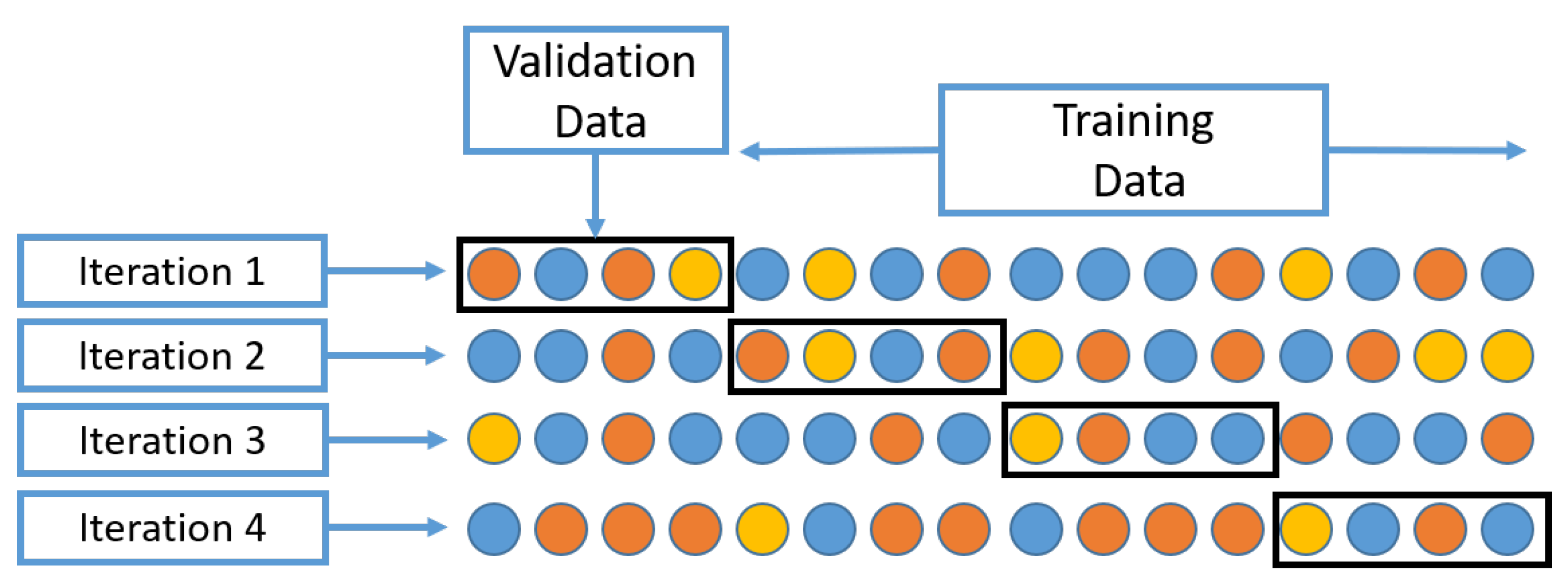
Cross-validation is used in this work to provide an up-front identification of the accuracy of a ROM and to identify the optimal regularization term, . In this work we are using k-fold cross validation, although other forms are available, such as exhaustive cross validation, leave-p-out cross validation, and leave-one-cross validation, among many more [21]. K-fold cross validation is a simple form of cross validation in which the set of available data is split into two portions, the training set and the validation set, with the number k referring to the number of groups the data are split into. A graphical representation is demonstrated in Figure 1.
The error function used during the cross validation is
where the matrix consists of a subset of the polynomial coefficient matrix from Equation (10) and the vector consists of the a subset of the nonlinear modal forces corresponding to the validation set as defined by the k-fold cross validation procedure. The polynomial coefficients, , are the polynomial coefficients subset of the coefficients estimated using the training set. The total error during cross-validation is found as
Once the scores are retained from the cross-validation stage, one is able to select the hyper-parameter, the lasso regularization parameter in this work, that provides the most accurate model. In the context of this work, the most accurate model is represented by the model which has the lowest mean squared error (MSE) during cross validation. In this work the MSE is used as the error metric for each k-split, but there are other options as well, such as median absolute error (MAE), which is less sensitive to outliers in the residual. There is potential that this error metric would produce an optimal model with different regularization parameter .
2.3.4. Discussion on Computational Cost
One disadvantage of such an approach is that it requires a larger number of nonlinear static load cases to generate the training data for a ROM compared to traditional IC method. However, this cost is offline and completely parallelizable, as each static load case can be computed independently of the others. Once the coefficients of the sparse ROM have been identified via LASSO, the computational cost of using the ROM in subsequent analyses—static solvers, time integrator, etc.—is comparable to that of a traditional IC ROM when both have a low number of modes included. As the number of modes in the basis set increases, the number of nonlinear terms increases in the order of cubically, resulting in a larger evaluation cost of the nonlinear force function Equation (6). The sparse ROM has the ability to reduce this cost with savings proportional to the sparsity of the resulting ROM. The computational savings are analogous to those of dense vs. sparse matrix multiplication.
As mentioned, the coordinate descent algorithm is used to solve the regularized regression problem of Equation (16). This is an iterative solver which for a design matrix of N samples by p parameters scales . As the number of modes (m) increases, the number of nonlinear stiffness terms, i.e., design parameters, increases , resulting in each iteration of the coordinate descent algorithm scaling with respect to modes as . It is also possible that for larger systems with many parameters that the number of iterations to converge will increase. Fortunately, the coordinate descent can be parallelized and some of this computational burden can be alleviated.
3. Numerical Examples
3.1. Flat Beam
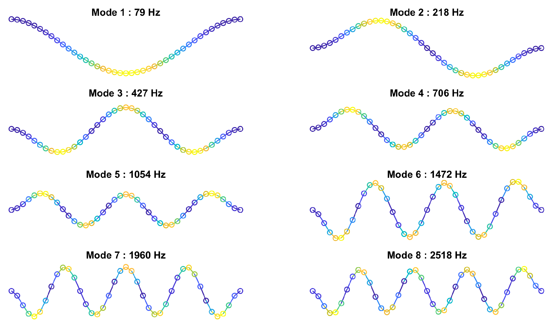
The first numerical study is a flat clamped-clamped beam that exhibits geometric nonlinearity. This beam has been used in numerous previous studies [22,23] to evaluate ROM building procedures. The beam has a length of 228.6 mm (9 in), a width of 12.7 mm (0.5 in), a thickness of 0.7874 mm (0.031 in), a modulus of elasticity of E = , a density of = , and a Poisson’s ratio of 0.29. The beam was modeled with 40 2-node beam elements and restrained to in-plane motion resulting in a total of 117 DOF. The first eight linear normal modes of the beam are presented in Figure 2. In this case a 2-DOF ROM is considered, consisting of the modes 1 and 3 of the flat beam. The ROM contains seven nonlinear stiffness terms per modal DOF, three quadratic, and four cubic, resulting in 14 total terms.
3.1.1. ROM Training and Nonlinear Stiffness Terms
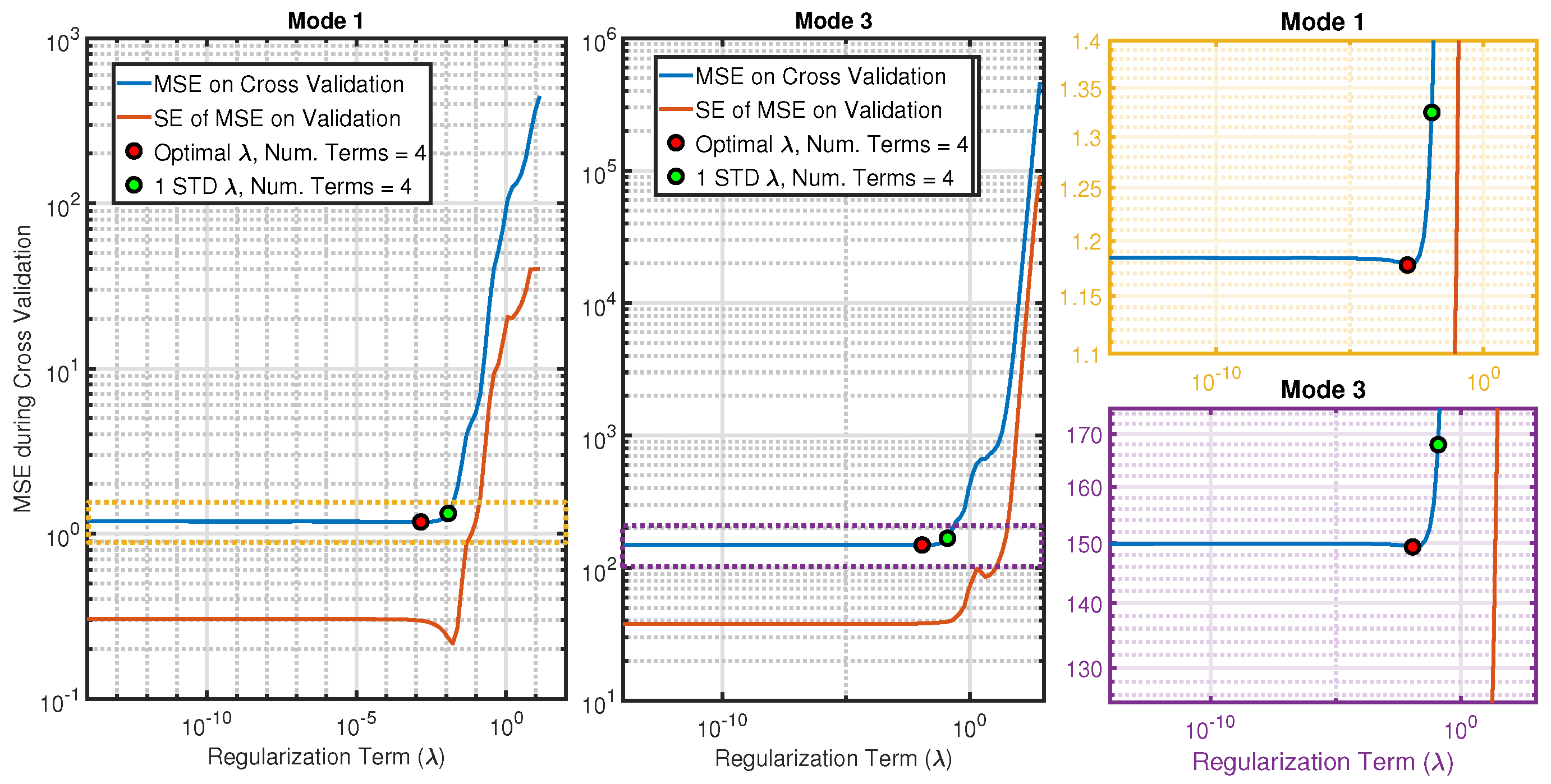
The training data for the flat beam ROM consisted of 10 separate sets of load case data, each of which contained eight load cases and was a complete set in that it contained all of the typical permutations of the modal loadings [22] and thus could have been used to obtain a single ROM with the conventional approach. The result was 80 total static load cases with the matrix from the linear system of equations presented in Equation (12) having size . The load scaling values for the forces used to excite the model were created from a normal distribution with a mean of and , where is the thickness of the beam (0.031 in). The cross-validation training results for the ROMs are presented in Figure 3. The MSE is plotted as a function of the regularization parameter. In both cases it was found that the optimal penalty term and the corresponding number of terms per modal DOF were both four, corresponding to a model that contains only the cubic terms. The actual decrease in MSE relative to the LS solution was less than in both cases, indicating that this model has an MSE that is nearly as low as a model with many more coefficients. The STD value identified on the plots can be used as a metric to determine how much MSE may be acceptable relative to the optimal model. For the flat beam case at hand, the sparsity did not change between the optimal model and model so there would be no benefit to using the model. For other application cases there could be large variations in the sparsity between the optimal and model in which it may be advantageous to use the sparser model and the point allows reference to amount of additional error associated with the model.
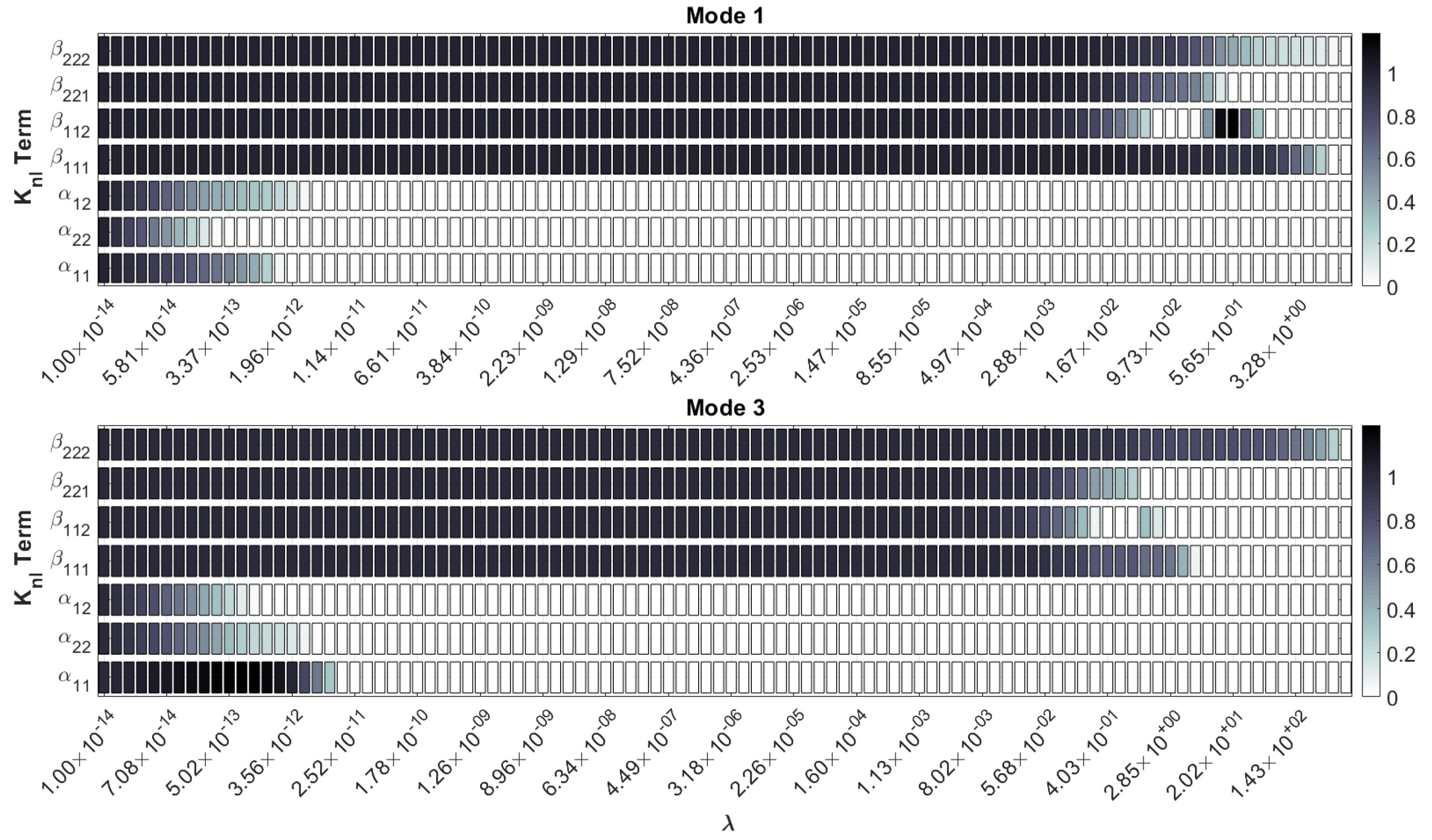
The nonlinear stiffness coefficients of the 2-DOF ROM identified via LASSO are presented in Figure 4. In each plot the nonlinear stiffness coefficients are normalized to the values identified using least squares regression. For the first modal equation, the terms that are removed first are the quadratic ones. Following that, the is removed but shortly after comes back into the solution as is removed. Then at a value of the only term to remain is the term. The sparse predictor models created via LASSO for the first modal equation correspond well with what is known about the beam. The quadratic terms are known to be negligible because the beam is flat and it makes sense that the most important term is the parameter. For the second modal equation the same trend was found, with the quadratic terms being removed early on and again the last term retained in the model being the cubic value associated with the second mode alone .
3.1.2. Evaluation of Accuracy
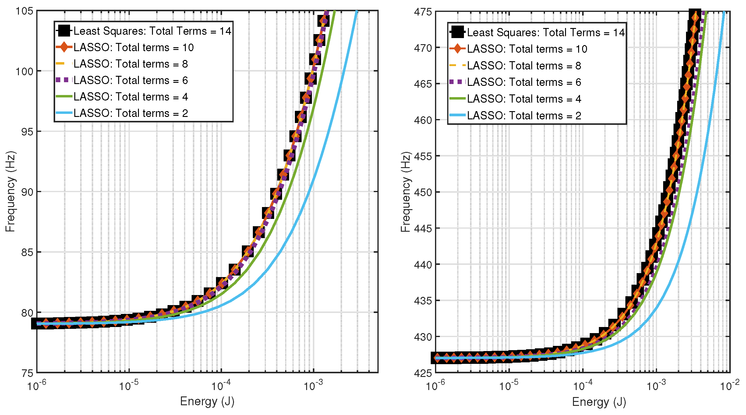
To evaluate the accuracy of the ROMs created using LASSO, the models were compared with the least squares model. The metrics used to compare the numerical models were the nonlinear normal modes (NNMs), which define the amplitude-frequency dependence of a nonlinear system, and hence enable a strong comparison between the ROMs [23,24]. The two NNMs of the numerical models, represented as frequency energy plots (FEPs), are shown in Figure 5. The NNMs were computed using the Multi-Harmonic Balance (MHB) method as in [25] with three harmonics included within the solution. The two-mode ROM created in this example contained only these two modes.
The ROMs made using LASSO were comparable with the NNM computed from the LS ROM. The LASSO ROMs remained accurate compared to the LS ROM for the first NNM when it was reduced down to six terms, or only of its original size. For the second NNM, the LASSO ROMs maintained accuracy when reduced down to eight nonlinear stiffness terms, or a sparsity value of . After less than eight terms were retained within the ROM, the NNM started to lose accuracy. This was expected because from Figure 3 the MSE during cross-validation increases after removing more than optimal number of terms, three per modal DOF, resulting in six in total removed. This simple example has shown that LASSO with cross-validation can identify those terms in a simple ROM that are most important, and that it produces results that agree with our expectations based on the physics of the problem. The next section tackles a more challenging problem.
3.2. Curved Panel
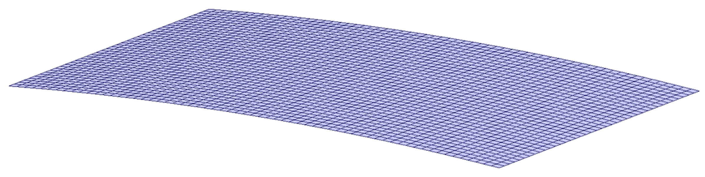
The second numerical study is on a curved panel, originally presented in [11] and also studied in [9]. The panel is 247.65 mm (9.75 in) by 400.05 mm (15.75) in along the curved direction which has a radius of curvature of 2540 mm (100 in). The panel has fixed boundary conditions along all sides. The finite element of the panel is shown in Figure 6 consisting of 63 elements along the curved direction and 24 along the flat direction. The panel is made of stainless steel with a modulus of elasticity of 204.8 GPa (28,500 ), poisson’s ratio of , and a density of = 7870 kg/m (7.48 × 10).
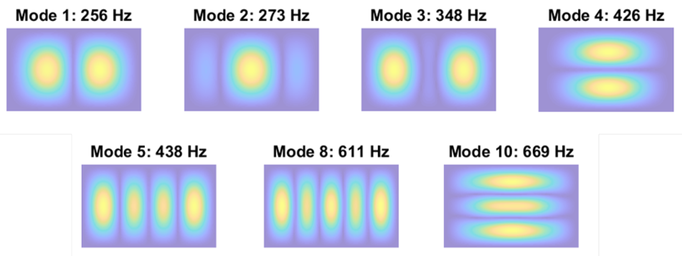
Based on insights in previous work [8], one must include a significant number of the symmetric bending modes in the basis set in order to accurately capture the response of the structure to a base excitation (equivalent to a uniform pressure load on the panel). The basis set for the largest reduced order model used for this structure consisted of modes 1, 2, 3, 4, 5, 8, and 10—seven modes in total. The linear modes of the structure used within the basis set are shown in Figure 7. This 7-mode ROM will be used in the evaluation of accuracy section to follow but due to the size of the ROM (112 stiffness terms per modal DOF resulting in 784 nonlinear stiffness terms total) it is difficult to portray the nonlinear stiffness terms and training results as was done in the previous section. For each ROM made, the load cases consisted of 10 observations of loading such that each case (378 static loads) contained enough information to generate a single ROM. The result is 3780 total static load cases with the matrix from the linear system of equations presented in Equation (12) having size . The scaling factors of each of the 10 observations were again sampled from a normal distribution with a mean of 1x the plate’s thickness and a standard deviation of 0.1× the thickness. Before showing those results, a 4-mode ROM consisting of modes 1, 2, 3, and 4 was used to demonstrate the training and nonlinear stiffness parameter identification.
3.2.1. Training and Nonlinear Stiffness Identification
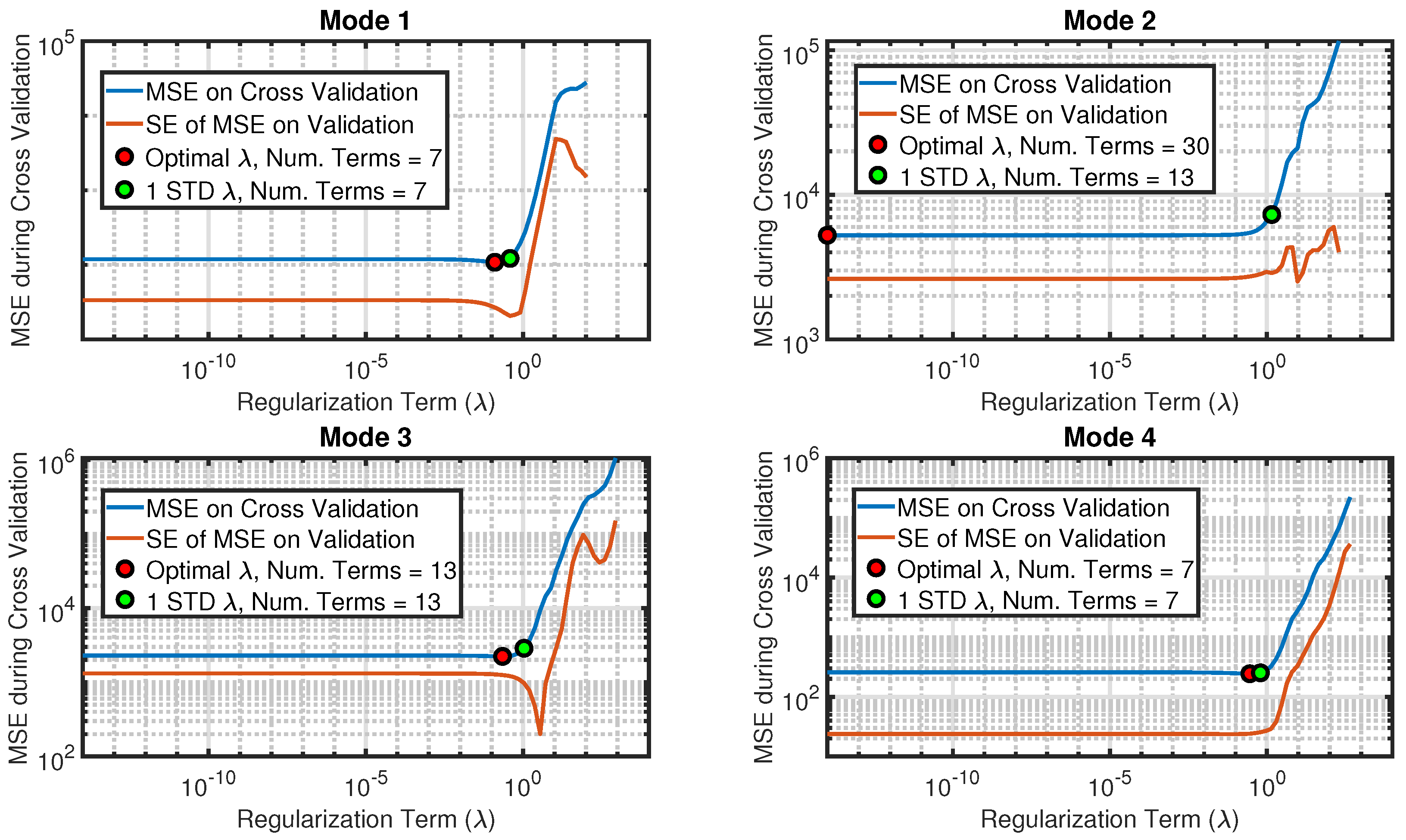
The cross-validation results when generating the a 4-mode ROM are presented in Figure 8 for each mode included within the ROM. The MSE of the k-fold cross validation is presented along with the standard error (SE) of the MSE for each value of . Furthermore, the optimal lambda is presented for each case. For each case the MSE is relatively constant from low values of lambda, corresponding to near least squares solutions, up until the optimal values for each mode. For modes 1, 3, and 4 the optimal values were near 1. For mode 2, the primary bending mode, the optimal corresponded to a or a least squares solution. For modes 1, 3, and 4 the optimal regularization coefficient occurs right before the model began to become inaccurate, because too many coefficients were removed.
Three sparsity plots are shown in Figure 9, showing the terms that would be retained and their relative magnitudes for three cases: (1) the least squares solution (all terms retained), (2) the optimal solution identified via cross-validation, and (3) a solution in which terms with the smallest magnitude are removed. The later is used to demonstrate that lasso does not simply remove the lowest magnitude prediction variables; the magnitude selection procedure removes different parameters from the model than LASSO does, and furthermore, if one were to perform a procedure in this manner, the parameters that are retained in the model would not be changed from the initial LS estimate and may not be optimal.
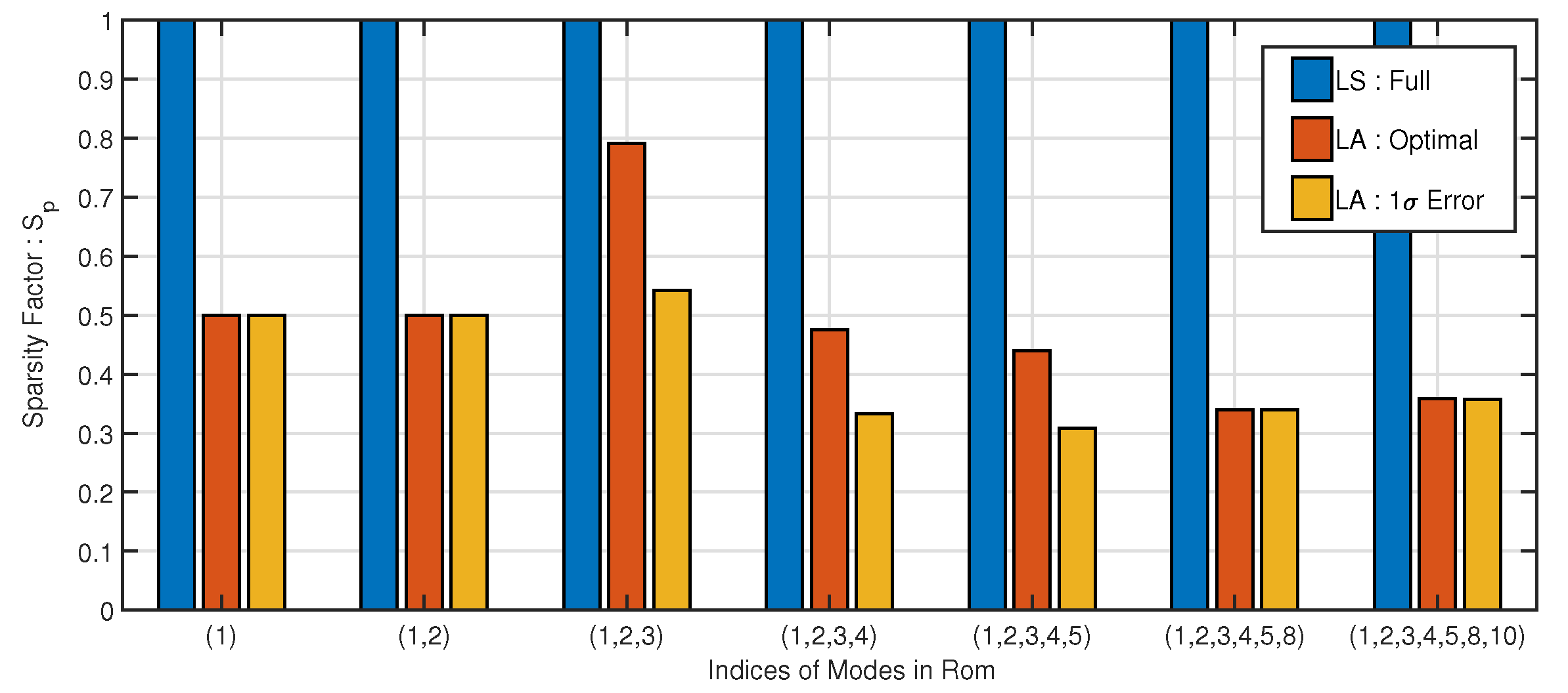
The same procedure was applied to ROMs from single mode up to the 7-mode ROM with modes (1–5,8,10) as described earlier, and the resulting sparsities for the optimal model and 1-standard deviation error models are presented in Figure 10. The sparsity parameter, , is the ratio of non-zero coefficients retained in the model to the number of total coefficients of the LS model. In each case the LASSO procedure identifies an optimal model, in terms of MSE during cross-validation, that is sparse. In many of the cases the error model produces a similar sparsity model as the optimal.
3.2.2. Dynamic Accuracy Evaluation
For this structure the dynamic accuracy was evaluated by computing NNMs of the ROM using the multi-harmonic balance method [25], projecting the response to the physical domain via the basis set to obtain an initial displacement, , and integrating the response over one period. The accuracy is then determined by the periodicity of the response as in [26], using the following definition,
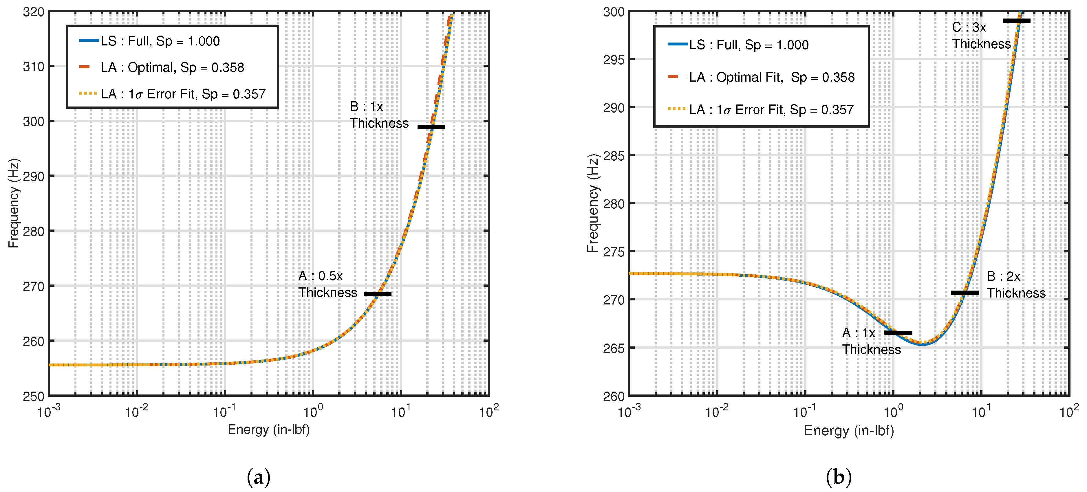
where is the displacement at the end of the integration over the period. This metric provides a measure of how well the NNM of the ROM captures the true NNM of the full FE model. The first two nonlinear normal modes of the curved panel are presented in Figure 11 in subplots (a) and (b) respectively. For both NNMs there is little discrepancy between the curves for each of the numerical models.
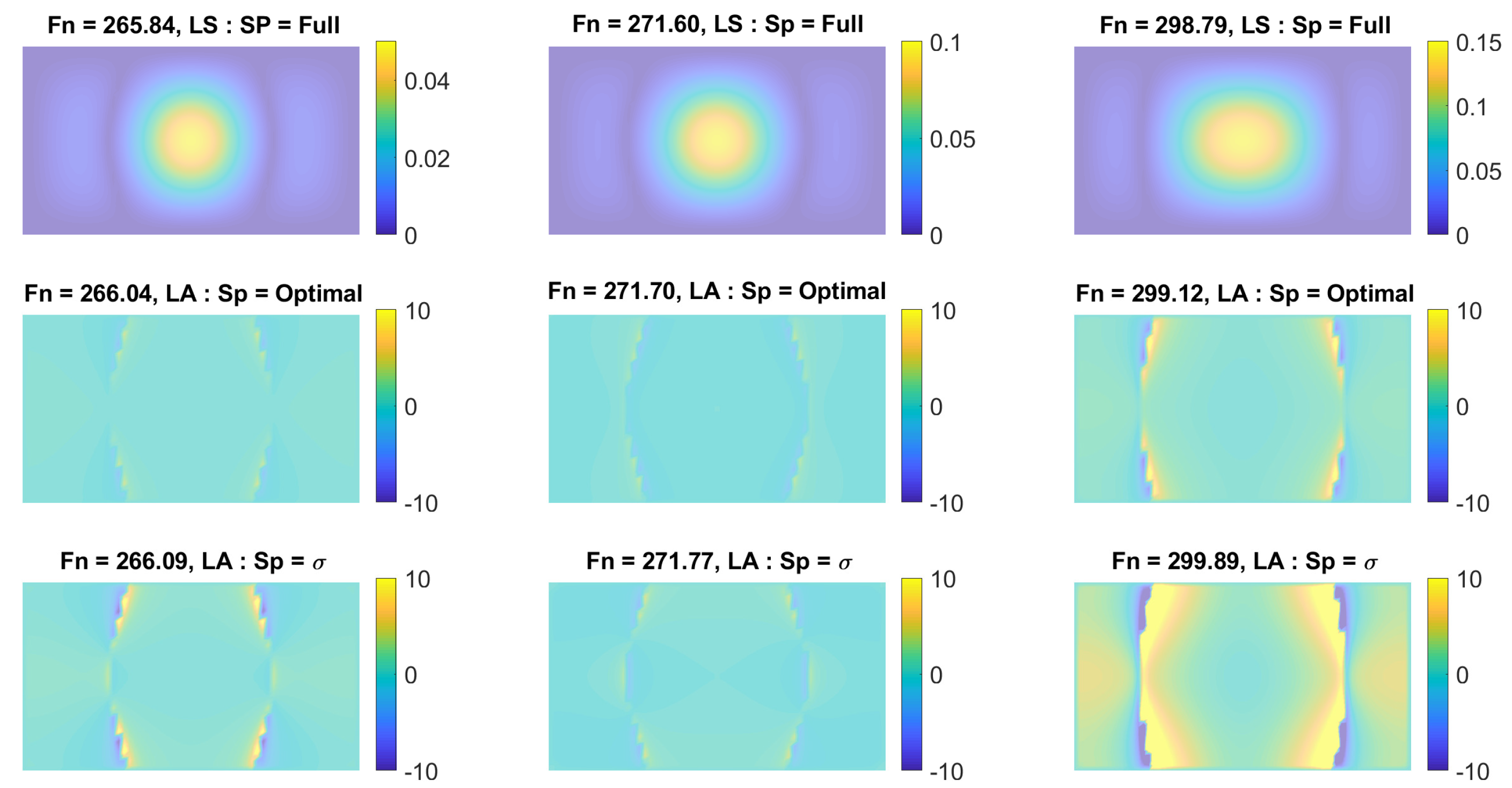
The displacements along the NNM at the points described in subplot(b) of Figure 11 for the full sparsity ROM model are presented in Figure 12 along the first row where the contour units are inches. The percent difference between the optimal sparsity ROM and the full sparsity ROM are plotted along the second row where the contour units are percent difference. In general the percent difference in the displacement field is low, less than 5%, for each solution except near the nodal lines of the mode. The percent difference between the sparsity ROM and the full sparsity ROM are plotted along the third row. In general the ROM does a good good at predicting the displacement field except at the third solution point near 300Hz where there are differences about 10% across a large portion of the model.
The periodicity metric for each of the points designated in Figure 11 for the second NNM are presented in Table 1 for each model. Additionally, the periodicity values from a model using a single set of load cases is presented to compare with previous ROM building approaches (e.g., in [17]). For example, when using least squares with all load cases, the periodicity value at point B is indicating that when the full FEM is integrated over one cycle using the initial conditions found by that ROM, the response of the full FEM is periodic with a maximum error of only . In contrast, using the authors’ prior approach (second row of Table 1), the error is more than two times higher at . Looking at the LASSO results, we see that, although the LS model performs better than the LASSO models at all three points along the NNM, the LASSO model with optimal MSE increases the periodicity error only very slightly and yet it has a sparsity value of 0.358, or is smaller. The model has larger error, especially at point C, where the maximum response amplitude is 3× the thickness of the structure. A value of NA is given at point C for the LS model, which was generated with only one set of data with load levels set to give a deformation of 1× the thickness, because the NNM computation algorithm was not able to converge up to that high of a response; often a faulty ROM cannot be integrated in time or shows instability for large displacements.
4. Conclusions
This work has demonstrated that simultaneous regression and selection via LASSO is an effective procedure to reduce the number nonlinear stiffness terms in a ROM while maintaining accurate response predictions. In particular, the procedure was applied to a well-characterized case study of a flat beam in which the procedure removed the known unimportant terms, the quadratic terms of the system.
Application of LASSO to the curved plate better demonstrated its benefit as a useful tool to help to identify the important nonlinear stiffness parameters of the ROM, which could not be predicted easily using physical arguments. In the 7-mode ROM case, the LASSO approach was able to reduce the number of coefficients by while maintaining accurate response predictions, as evaluated by using nonlinear normal modes. Even then, the level of reduction achieved was far less than was possible for the flat beam; this deserves further investigation in a future study.
Furthermore, a procedure has been developed and applied to the systems at hand using a data-driven approach to alleviate the need to identity optimal scaling factors for the load cases used to generate the ROM. This procedure is enhanced by using cross-validation during the training stage to evaluate the accuracy of the ROM. In both cases, the results showed that the larger MSE during cross-validation corresponded to less accurate ROMs in terms of their NNMs, supporting the use of cross-validation as a metric to evaluate the ROMs.
Author Contributions
Conceptualization, C.V.D., and M.A.; methodology, C.V.D., A.M., M.A. and J.H.; software, C.V.D. and A.M.; formal analysis, C.V.D. and A.M.; investigation, C.V.D. and A.M.; writing—original draft preparation, C.V.D., A.M. and M.A.; writing—review and editing, C.V.D., A.M., M.A. and J.H.; supervision, M.A. and J.H. All authors have read and agreed to the published version of the manuscript.
Funding
This research was funded by the Air Force Office of Scientific Research, Award # FA9550-17-1-0009, under the Multi-Scale Structural Mechanics and Prognosis program managed by Jaimie Tiley.
Institutional Review Board Statement
Not applicable.
Informed Consent Statement
Not applicable.
Conflicts of Interest
The authors declare no conflict of interest.
References
- Cook, R.D.; Malkus, D.S.; Plesha, M.E.; Witt, R.J. Concepts and Applications of Finite Element Analysis; Wiley: New York, NY, USA, 1974; Volume 4. [Google Scholar]
- Shi, Y.; Mei, C. A Finite Element Time Domain Modal Formulation for Large Amplitude Free Vibrations of Beams and Plates. J. Sound Vib. 1996, 193, 453–464. [Google Scholar] [CrossRef]
- Muravyov, A.A.; Rizzi, S.A. Determination of nonlinear stiffness with application to random vibration of geometrically nonlinear structures. Comput. Struct. 2003, 81, 1513–1523. [Google Scholar] [CrossRef]
- Perez, R.; Wang, X.Q.; Mignolet, M.P. Nonintrusive structural dynamic reduced order modeling for large deformations: Enhancements for complex structures. J. Comput. Nonlinear Dyn. 2014. [Google Scholar] [CrossRef]
- Mignolet, M.; Przekop, A.; Rizzi, S.; Spottswood, M. A review of indirect/non-intrusive reduced order modeling of nonlinear geometricstructures. J. Sound Vib. 2013, 332, 2437–2460. [Google Scholar] [CrossRef]
- McEwan, M.; Wright, J.; Cooper, J.; Leung, A. Combined Modal/Finite Element Analysis Technique for the Dynamic Response of a Non-linear Beam to Harmonic Excitation. J. Sound Vib. 2001, 243, 601–624. [Google Scholar] [CrossRef]
- McEwan, M.; Wright, J.; Cooper, J.; Leung, A. A finite element/modal technique for nonlinear plate and stiffened panel response prediction. In Proceedings of the 19th AIAA Applied Aerodynamics Conference, Anaheim, CA, USA, 11–14 June 2001; p. 1595. [Google Scholar]
- Hollkamp, J.J.; Spottswood, M.S.; Gordon, R.W. Nonlinear modal models for sonic fatigue response prediction: A comparison of methods. Sound Vib. 2005, 284, 1145–1163. [Google Scholar] [CrossRef]
- Hollkamp, J.J.; Gordon, R.W. Modeling Membrane Displacements in the Sonic Fatigue Response Prediction Problem. In Proceedings of the 46th AIAA/ASME/ASCE/AHS/ASC Structures, Structural Dynamics and Materials Conference, Austin, TX, USA, 18–21 April 2005. [Google Scholar]
- Rizzi, S.A.; Przekop, A. System identification-guided basis selection for reduced-order nonlinear response analysis. J. Sound Vib. 2008, 315, 467–485. [Google Scholar] [CrossRef]
- Gordon, R.W.; Hollkamp, J.J. Reduced-Order Models for Acoustic Response Prediction; Technical, Tech Report: AFRL-RB-WP-TR-2011-3040; Air Force Research Laboratory, Wright-Patterson AFB: Dayton, OH, USA, 2011. [Google Scholar]
- Nicolaidou, E.; Melanthuru, V.R.; Hill, T.L.; Neild, S.A. Accounting for Quasi-Static Coupling in Nonlinear Dynamic Reduced-Order Models. J. Comput. Nonlinear Dyn. 2020, 15. [Google Scholar] [CrossRef]
- Shen, Y.; Béreux, N.; Frangi, A.; Touzé, C. Reduced order models for geometrically nonlinear structures: Assessment of implicit condensation in comparison with invariant manifold approach. Eur. J. Mech. A/Solids 2021, 86, 104165. [Google Scholar] [CrossRef]
- Wang, X.; Mignolet, M.P. Uncertainty Quantification of Nonlinear Stiffness Coefficients in Non-Intrusive Reduced Order Models. In Proceedings of the 38th International Modal Analysis Conference (IMAC XXXVIII), Orlando, FL, USA, 10–13 February 2020. [Google Scholar]
- Dong, H.; Chen, K.; Linderoth, J. Regularization vs. Relaxation: A conic optimization perspective of statistical variable selection. arXiv 2015, arXiv:1510.06083. [Google Scholar]
- Tibshirani, R. Regression shrinkage and selection via the lasso. J. R. Stat. Soc. Ser. (Methodol.) 1996, 58, 267–288. [Google Scholar] [CrossRef]
- Kuether, R.J.; Deaner, B.; Hollkamp, J.J.; Allen, M.S. Evaluation of Geometrically Nonlinear Reduced-Order Models with Nonlinear Normal Modes. AIAA J. 2015, 53, 3273–3285. [Google Scholar] [CrossRef]
- VanDamme, C.I.; Allen, M.S. Using nnms to evaluate reduced order models of curved beam. In Rotating Machinery, Hybrid Test Methods, Vibro-Acoustics & Laser Vibrometry, Volume 8; Springer: Berlin/Heidelberg, Germany, 2016; pp. 457–469. [Google Scholar]
- Boyd, S.; Vandenberghe, L. Convex Optimization; Cambridge University Press: New York, NY, USA, 2004. [Google Scholar]
- Friedman, J.; Hastie, T.; Tibshirani, R. Regularization paths for generalized linear models via coordinate descent. J. Stat. Softw. 2010, 33, 1. [Google Scholar] [CrossRef] [PubMed] [Green Version]
- Refaeilzadeh, P.; Tang, L.; Liu, H. Cross-Validation. In Encyclopedia of Database Systems; Liu, L., Özsu, M.T., Eds.; Springer: Boston, MA, USA, 2009; pp. 532–538. [Google Scholar]
- Gordon, R.; Hollkamp, J. Reduced-Order Models for Acoustic Response Prediction of a Curved Panel. In Proceedings of the 52nd AIAA/ASME/ASCE/AHS/ASC Structures, Structural Dynamics and Materials Conference, Structures, Structural Dynamics, and Materials and Co-located Conferences, Denver, CO, USA, 4–7 April 2011. [Google Scholar] [CrossRef]
- Kuether, R.J.; Allen, M.S. Validation of Nonlinear Reduced Order Models with Time Integration Targeted at Nonlinear Normal Modes. In Nonlinear Dynamics, Volume 1; Conference Proceedings of the Society for Experimental Mechanics Series; Springer: Cham, Switzerland, 2016. [Google Scholar]
- Kerschen, G.; Peeters, M.; Vakakis, A.F.; Golinval, J.C. Nonlinear normal modes, Part I: A useful framework for the structural dynamicist. Mech. Syst. Signal Process. 2009, 23, 170–194. [Google Scholar] [CrossRef] [Green Version]
- VanDamme, C.I.; Moldenhauer, B.; Allen, M.S.; Hollkamp, J.J. Computing Nonlinear Normal Modes of Aerospace Structures Using the Multi-harmonic Balance Method. In Nonlinear Dynamics, Volume 1; Springer: Berlin/Heidelberg, Germany, 2018; pp. 247–259. [Google Scholar]
- Kuether, R.J.; Allen, M.S. A numerical approach to directly compute nonlinear normal modes of geometrically nonlinear finite element models. Mech. Syst. Signal Process. 2014, 46, 1–15. [Google Scholar] [CrossRef]
Figure 1.
Graphical depiction of k-fold cross validation with 4 folds.

Figure 2.
Linear normal modes of the flat beam. Modes 1 and 3 are used within the base set.

Figure 3.
Mean squared error (MSE) and standard error (SE) of a 1,3-mode reduced order model (ROM) when using k-fold cross validation for each value. The two subplots on the right are zoomed in portions of the plots on the left and center.
Figure 3.
Mean squared error (MSE) and standard error (SE) of a 1,3-mode reduced order model (ROM) when using k-fold cross validation for each value. The two subplots on the right are zoomed in portions of the plots on the left and center.

Figure 4.
Nonlinear stiffness coefficients of the first and third modal equations versus the least absolute selection and shrinkage (LASSO) regularization parameter . The nonlinear stiffness coefficients were normalized with respect to the values estimated using least squares.
Figure 4.
Nonlinear stiffness coefficients of the first and third modal equations versus the least absolute selection and shrinkage (LASSO) regularization parameter . The nonlinear stiffness coefficients were normalized with respect to the values estimated using least squares.

Figure 5.
Frequency energy plot of the first (left) and third (right) nonlinear normal modes (NNMs) of the flat beam for ROMs created using least squares and using LASSO with various penalty terms.
Figure 5.
Frequency energy plot of the first (left) and third (right) nonlinear normal modes (NNMs) of the flat beam for ROMs created using least squares and using LASSO with various penalty terms.

Figure 6.
Finite element model of the curved panel.

Figure 7.
Shapes of the linear modes included in the basis set for the ROM used in this study.

Figure 8.
Mean squared error (MSE) and standard error (SE) of k-fold cross validation for each value.
Figure 8.
Mean squared error (MSE) and standard error (SE) of k-fold cross validation for each value.

Figure 9.
Nonlinear stiffness coefficient matrices for three different sets of sparsity approaches: (1) The least squares solution (all terms shown would be retained), (2) the optimal solution identified via cross-validation (terms in white are eliminated), and (3) a solution in which terms with the smallest magnitude are removed (terms in white are eliminated). The colorbar gives the log of the stiffness term; values below are zero.

Figure 10.
Bar plot depicting the sparsity factors for various orders of ROMs.

Figure 11.
Nonlinear normal modes of the curved panel computed from ROM with modes 1, 2, 3, 4, 5, 8, and 10 included within the basis set. Subplot (a), NNM of first mode. Subplot (b), NNM of the second mode. NNMs were computed using the Multi-Harmonic Balance (MHB) method with 5 harmonics included.
Figure 11.
Nonlinear normal modes of the curved panel computed from ROM with modes 1, 2, 3, 4, 5, 8, and 10 included within the basis set. Subplot (a), NNM of first mode. Subplot (b), NNM of the second mode. NNMs were computed using the Multi-Harmonic Balance (MHB) method with 5 harmonics included.

Figure 12.
The first row of contours are the full finite element (FE) model displacements at the NNM solutions designated in Figure 11 for the full ROM model. The second row of contours are the percentage differences in the displacements fields of the optimal model with respect to the full model. The third row of contours are the percentage differences in the displacement fields of the optimal model with respect to the full model.


Publisher’s Note: MDPI stays neutral with regard to jurisdictional claims in published maps and institutional affiliations. |
© 2021 by the authors. Licensee MDPI, Basel, Switzerland. This article is an open access article distributed under the terms and conditions of the Creative Commons Attribution (CC BY) license (http://creativecommons.org/licenses/by/4.0/).
Share and Cite
MDPI and ACS Style
Van Damme, C.; Madrid, A.; Allen, M.; Hollkamp, J. Simultaneous Regression and Selection in Nonlinear Modal Model Identification. Vibration 2021, 4, 232-247. https://0-doi-org.brum.beds.ac.uk/10.3390/vibration4010016
AMA Style
Van Damme C, Madrid A, Allen M, Hollkamp J. Simultaneous Regression and Selection in Nonlinear Modal Model Identification. Vibration. 2021; 4(1):232-247. https://0-doi-org.brum.beds.ac.uk/10.3390/vibration4010016
Chicago/Turabian StyleVan Damme, Christopher, Alecio Madrid, Matthew Allen, and Joseph Hollkamp. 2021. "Simultaneous Regression and Selection in Nonlinear Modal Model Identification" Vibration 4, no. 1: 232-247. https://0-doi-org.brum.beds.ac.uk/10.3390/vibration4010016