Article

Computational Analysis of the Active Control of Incompressible Airfoil Flutter Vibration Using a Piezoelectric V-Stack Actuator

by
Carmelo Rosario Vindigni
1,
Calogero Orlando
2,* and
Alberto Milazzo
3
1
Independent Researcher, 97015 Modica, Italy
2
Faculty of Engineering and Architecture, Kore University of Enna, 94100 Enna, Italy
3
Department of Civil, Environmental, Aerospace, and Materials Engineering—DICAM, Università degli Studi di Palermo, 90133 Palermo, Italy
*
Author to whom correspondence should be addressed.
Submission received: 6 February 2021 / Revised: 22 March 2021 / Accepted: 29 March 2021 / Published: 9 April 2021

Abstract

:
The flutter phenomenon is a potentially destructive aeroelastic vibration studied for the design of aircraft structures as it limits the flight envelope of the aircraft. The aim of this work is to propose a heuristic design of a piezoelectric actuator-based controller for flutter vibration suppression in order to extend the allowable speed range of the structure. Based on the numerical model of a three degrees of freedom (3DOF) airfoil and taking into account the FEM model of a V-stack piezoelectric actuator, a filtered PID controller is tuned using the population decline swarm optimizer P D S O algorithm, and gain scheduling (GS) of the controller parameters is used to make the control adaptive in velocity. Numerical simulations are discussed to study the performance of the controller in the presence of external disturbances.

1. Introduction

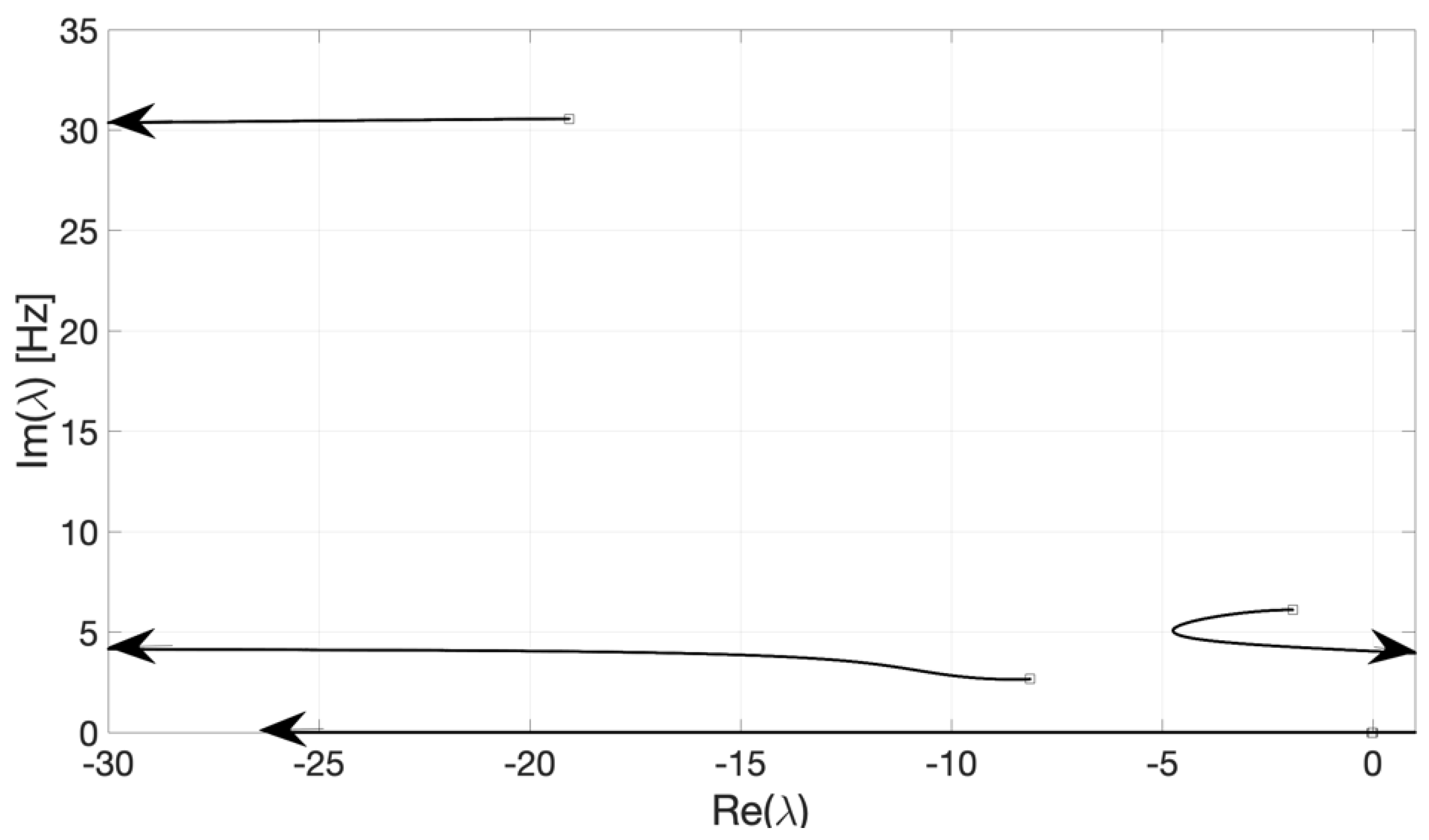
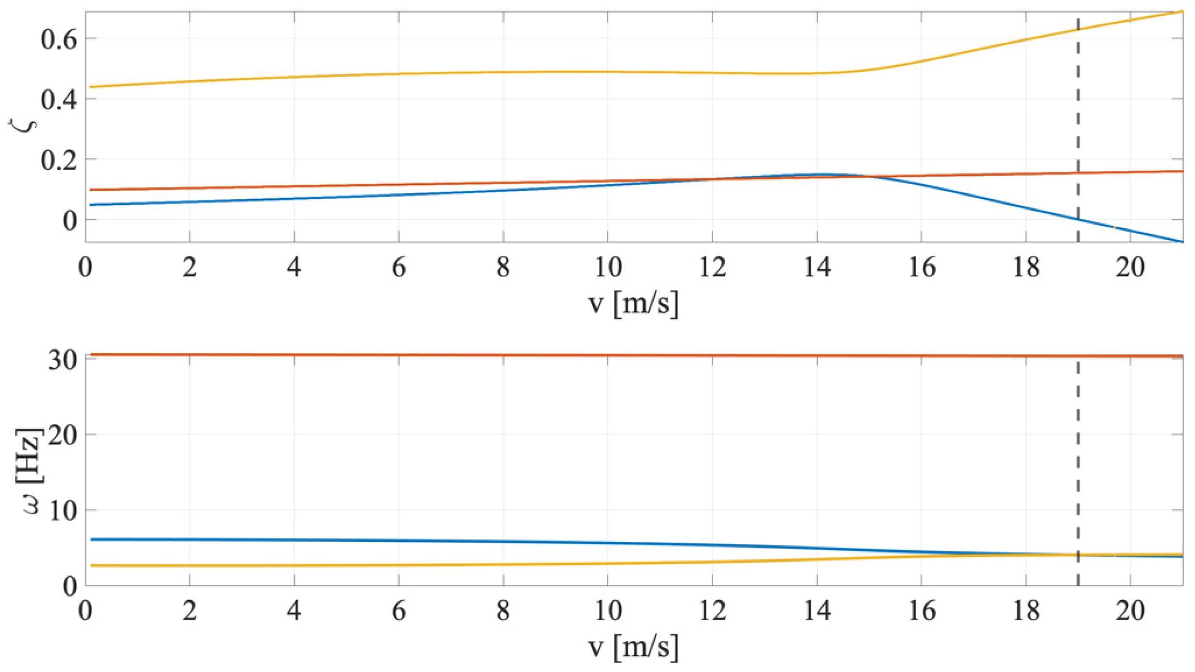
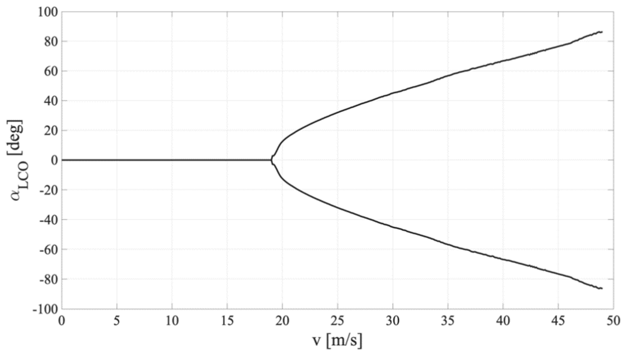
The flutter phenomenon is a dynamic instability that arises in lifting structures. It starts when the velocity becomes greater than a critical speed value, namely the flutter boundary. The fluid does not absorb the structure’s energy anymore but increases it as the damping becomes negative in value, causing a condition of fatigue or damage to the structure. The amplitude of the flutter oscillations can grow indefinitely in the linear model, particularly for divergent flutter, or reach a constant amplitude, such as with limit cycle oscillations (LCOs), when there are stiffness or aerodynamic nonlinearities, like in the actual case. By studying the variation of the damping ratio with the airstream velocity, it is possible to recognize different types of flutter [1] such as soft flutter, which is characterized by a slight slope of the damping ratio–speed curve, and hard flutter, which presents an abrupt variation of the damping ratio beyond the critical point and the hump mode, which is characterized by an initial reduction of damping that becomes negative in value and then increases to become positive again, describing a closed flutter region. The danger in reaching flutter instability is not only related to the high amplitude that can be encountered, but also to the fatigue effect and the increase of the control surface’s freeplay that it can cause. Over the years, many measures have been taken to prevent the rise of aeroelastic vibration phenomena. These can be mainly divided into two categories: passive and active methods. The study of mass balance belongs to the category of passive methods. The dimension and the position of masses strongly influence the amplitude and the frequency of flutter oscillations and modify the coupling mechanism between the bending and torsional vibration modes. A possible passive solution may be reached by moving the center of mass of each structural element of the wing closer to the axis of elasticity (AE) or by installing some concentrated masses to modify the wing’s moment of inertia, with the aim of reducing the amount of energy extracted from the fluid [2]. The modern methods used for flutter suppression are active methods. These use the data recorded from sensors installed on the structure, such as accelerometers, that are elaborated by a control system to properly move some aerodynamic surfaces or to implement other changes in the structure shape in order to obtain the desired dynamic behavior. The first examples of technology for the control of aeroelastic oscillations were based on the movement of aerodynamic surfaces, such as the trailing edge flap, by means of servo-hydraulic systems [3]. However, hydraulic systems present some drawbacks, such as the multiple conversions of the energy from one type to another, (e.g., from mechanical to hydraulic and to mechanical again). Conversions of energy lead to losses which, in turn, require higher nominal power of the system and higher weight as well. Lastly, it has to be said that hydraulic systems usually do not reach high bandwidth values. Thus, considering that aeroelastic phenomena are characterized by high frequencies, it follows that they might not be suitable for flutter suppression. The above-mentioned problems have motivated a growing interest in deformation-induced actuators, such as piezoelectric actuators. These, in fact, allow one to obtain mechanical power directly from electric energy. However, piezoelectric actuation does not allow for obtaining large displacements; thus, amplification mechanisms are to be studied. The first attempts of piezoelectric actuation were related to the use of bimorph beams realized by bonding two piezoelectric layers such that when an electric voltage is applied, one stretches while the other contracts, and bending deformations of the beam are obtained. Applications of this technology have been studied for the active control of helicopter blade twist by Waltz and Chopra [4] and for the flutter suppression of cantilever wings by Heeg [5]. An innovative method for wing oscillation control consists of the integration of actuators into the structure such that the geometry of the structure itself can be modified, usually in terms of the airfoil camber. This technology is called morphing actuation and has been studied since the 1990s, a period in which greater knowledge of piezoelectric materials was acquired, allowing the modeling of these materials in thin patches that can be integrated into the structure. The first studies that aimed at verifying the feasibility of piezoelectric morphing actuation were carried out by Lazarus et al. [6] along with numerous other scholars. However, they focused on the realization of all-movable aerodynamic surfaces not specifically designed for aeroelastic suppression. On the contrary, the technology presented by Fichera et al. [7] was specifically designed for aeroelastic suppression. They proposed a trailing edge morphing actuator capable of a 25 Hz bandwidth and a ±15° maximum equivalent rotation. It is made of two panels: one is an Macro-Fiber Composite-MFC piezo patch sandwich, which is the active part of the actuator, while the other is made of an aluminum alloy. Both panels are fixed on the wing box on one end and on a slider on the other end. In particular, the slider has airfoil trailing edge geometry and allows the two panels to slide in the deformed configuration. Other works dealing with piezoelectric actuation for aeroelastic suppression are based on the installation of piezo patches on the structure’s surface. The actuation of the patches is combined with modern control techniques in order to obtain a robust suppression system [8].
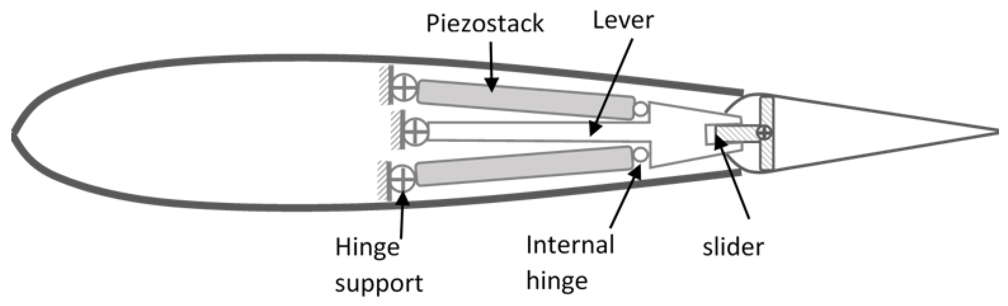
Other simpler configurations of piezoelectric actuation deal with the use of piezoelectric stacks. Piezo stacks are made by overlapping several piezoelectric layers in order to obtain a rod able to elongate or compress after the application of an electric voltage. Since this configuration does not allow one to obtain large displacements, some amplification mechanisms have been studied. Among others, there are the so-called X and V configurations. The mechanism presented by Hall and Prechtl [9] is based on an X configuration that allows amplification of the compression deformation of the stacks, resulting in a vertical displacement. On the other hand, the amplification mechanism proposed by Ardelean and Clark [10] takes advantage of two piezoelectric stacks arranged in a V configuration. The latter configuration is the one selected for the investigation carried out in the present study.
In order to realize the flutter suppression of the airfoil, using the movement of aerodynamic surfaces, many studies have been carried out over the years, and some solutions were reported in the following. In the work of Chen et al. [11], a two-degrees-of-freedom airfoil was considered, while the presence of both the leading edge and trailing edge aerodynamic surfaces was taken into account only in the expressions of the aerodynamic loads. The control method used by Chen et al. [11] was based on a sliding mode controller (SMC) (i.e., a nonlinear state feedback controller capable of changing its own structure when the system assumes different states). Thus, this controller presents robustness properties to external disturbances and uncertainties. However, the conventional SMC assumes that the controller could switch from one value to another instantaneously, and this is not possible in real-life applications due to the presence of delays. Therefore, the same authors proposed a high-order sliding mode controller (HOSMC) that was introduced after the backstepping procedure. In this way, a continuous input is provided to the controller [12]. In the studies of Na et al. [13] and Yang et al. [14], the model of a three-degrees-of-freedom airfoil was taken into account. Thus, the dynamic of the aerodynamic surface was considered. The control strategy proposed by Na et al. [13] was based on an LQR control implementing full-state feedback. Again, this leads to the necessity of having a system that is completely observable. The authors introduced the presence of measure noises and output disturbances, and thus a linear quadratic Gaussian (LQG) controller associated with a sliding mode observer has been implemented, since this architecture is capable of noise decoupling and shows robustness properties to disturbances. Yang et al. [14] instead specified that the LQR and LQG controllers are based on mathematical knowledge of the disturbances. Thus, when there are some uncertainties, these strategies lose robustness. In order to take into account the uncertainties in the design of the controller, Yang et al. [14] proposed H loop shaping, which is implemented by defining a generalized plant that encloses all the dynamic features to be controlled, such as sensors and actuator dynamics and so on, and introducing two different input vectors, namely the control input vector and the exogenous input vector. Then, the disturbance–output transfer function is defined, and the minimization problem of its infinity norm is solved. In the works of Wang et al. [15] and Zhang et al. [16], neural networks were associated with a full-state feedback–feedforward controller. This strategy has been studied by Bemelli-Zazzera et al. [17], too. They introduced the use of dynamic neural networks that were capable of changing their own weights through active training in order to adapt to the parameter variation during the normal functioning of the system. In the work of Andrievsky et al. [18], simple adaptive control (SAC) was implemented for the flutter suppression of an airfoil using an implicit reference model (IRM) and the pacification theorem. The authors implemented an adaptive control capable of flutter suppression in both the cases of the presence of actuator delays and the lack thereof.
Recent works dealing with active flutter suppression, carried out in the framework of projects financed by the European Union and the USA, have been presented. In the work carried out by Takarics and Vanek [19], a low-order, control-oriented LPV model of the aircraft was obtained using the bottom-up approach. The order of the nonlinear aeroservoelastic model subsystems is reduced, paying attention to capture accurately the flutter modes. Then, the controller is designed considering a polytopic LPV representation. In the work proposed by Waitman and Marcos [20], a high-fidelity, nonlinear aeroservoelastic model of the FLEXOP aircraft was considered, and three H optimal controllers were tuned and scheduled for different true airspeed values, increasing the damping of the flutter modes at these velocities. This approach led to a flutter boundary increase of 30%. Another recent work carried out by Theis et al. [21] dealt with the flutter suppression of the mini MUTT aircraft model, built at the University of Minnesota. The H loop shaping method was used in order to design a controller that presented good robustness to a wide variety of uncertainties. Pusch [22] studied a method based on the blending of control inputs and measurement outputs to isolate individual aeroelastic modes in order to use SISO controllers. In Schmidt et al. [23], the authors presented a study on drone flight dynamics, taking into account aeroelastic effects modeled by using the mean–axis formulation and quasi-steady aerodynamics. The rigid and aeroelastic model of the drone has since been used to study several controllers for autopiloting, considering the flutter instability as well.
In this work, one of the objectives is to present an FEM model of a V-stack piezoelectric actuator for the flutter suppression of an airfoil. Thus, the finite element model of the actuator is first introduced, and the behavior of the FEM model is compared with the experimental data in order to validate it. The second aim is to propose a heuristic method called population decline swarm optimization for tuning a simple control strategy based on a filtered PID controller by looking for the minimization of the integral of time absolute error (ITAE). This approach is used to set gain scheduling of the controller parameters in order to realize a velocity-dependent flutter suppression system and extend the flight envelope of the airfoil.
This paper is organized as follows. In Section 2, the numerical model of a three-degrees-of-freedom airfoil is described, and the augmented state space model for the time domain analysis is introduced. In 
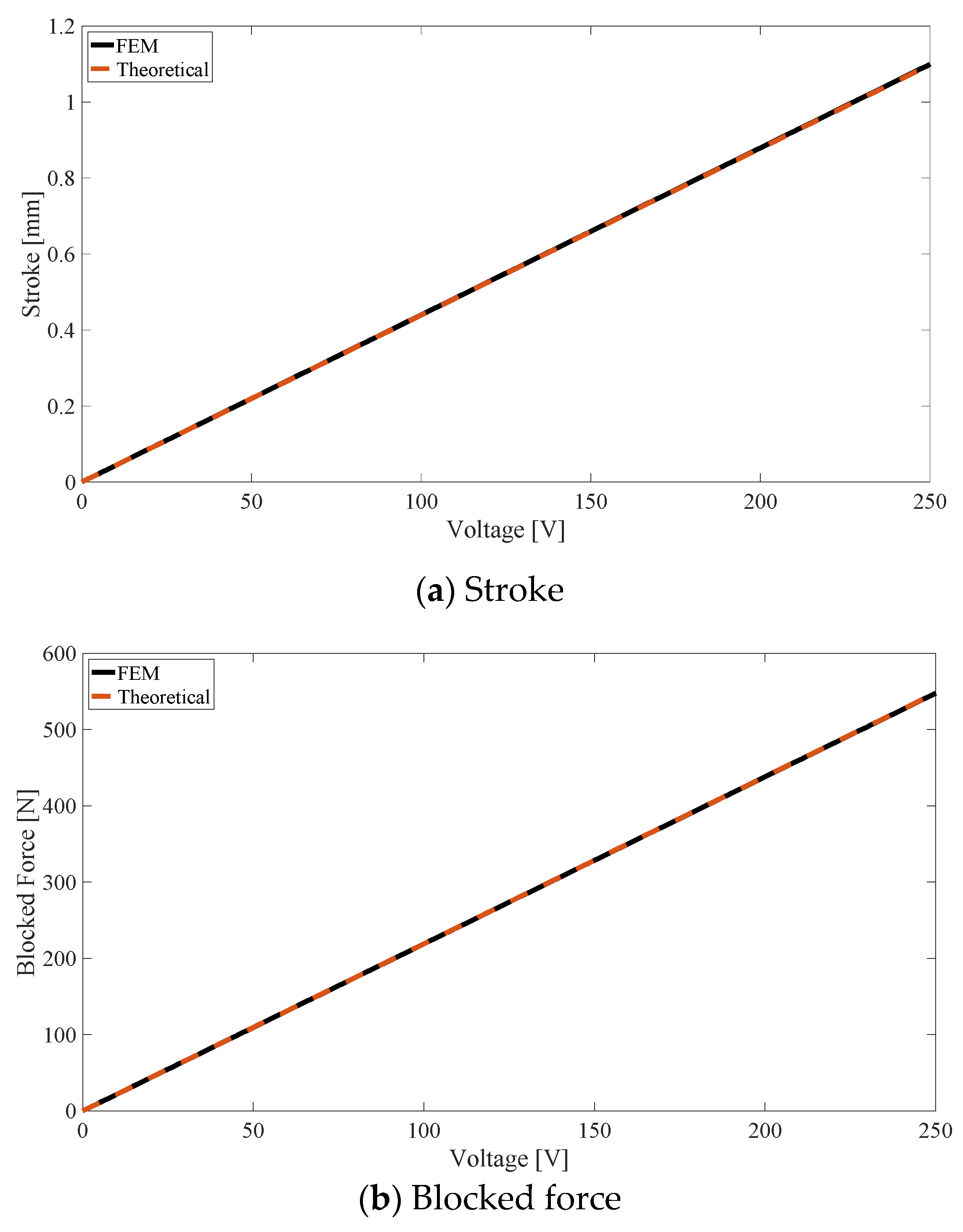
Section 3, the actuator is studied, introducing the finite element formulation of the piezo stacks. Starting from the state space model, the transfer function that relates the actuator tip’s vertical displacement to the input voltage is computed. In Section 4, the tuning of the gain scheduling-filtered PID controller is done. The filtered PID controller is tuned using the P D S O algorithm by minimizing the ITAE of the error of the pitch angle. In order to set up an adaptive control in the velocity, the gain scheduling approach is introduced, and the optimization algorithm is used to find the optimal controllers for different velocity values. In 
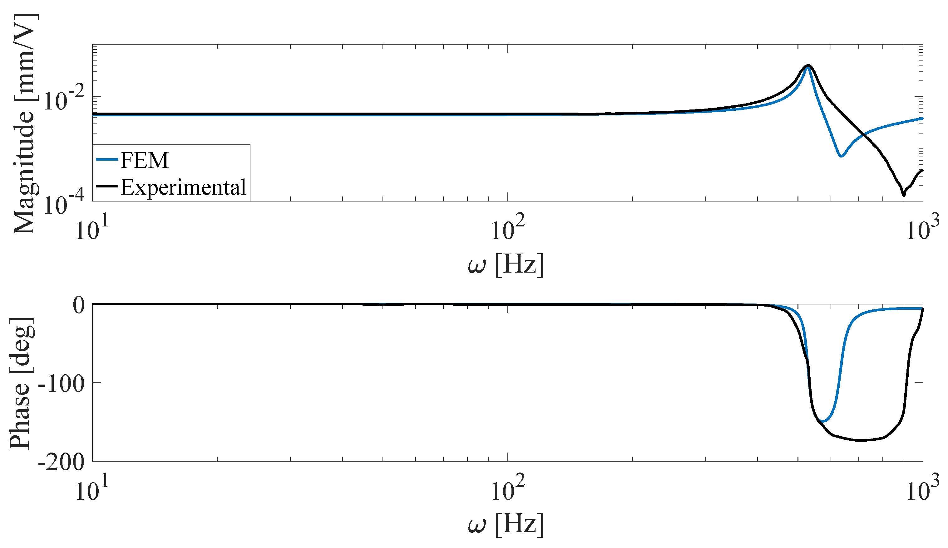
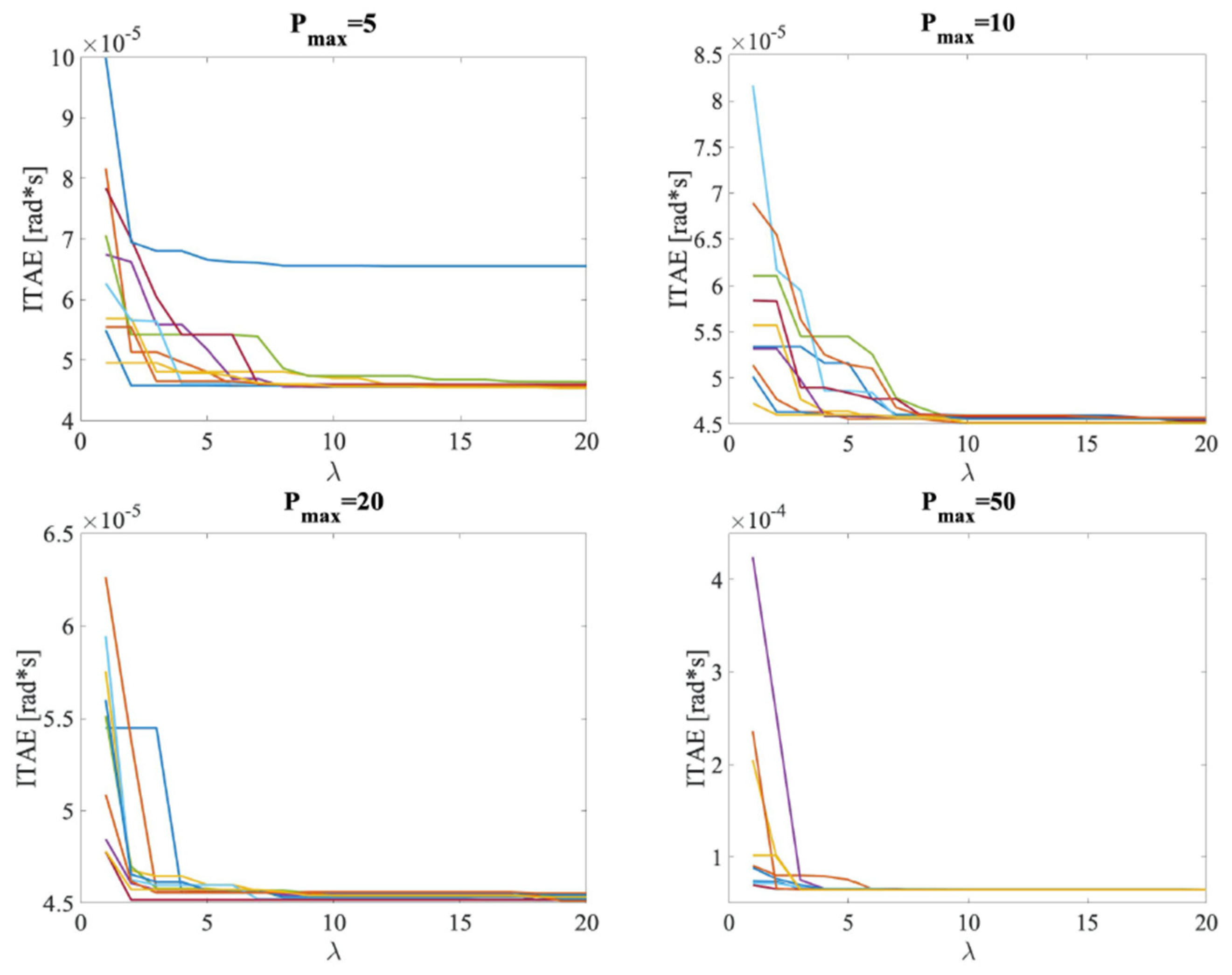
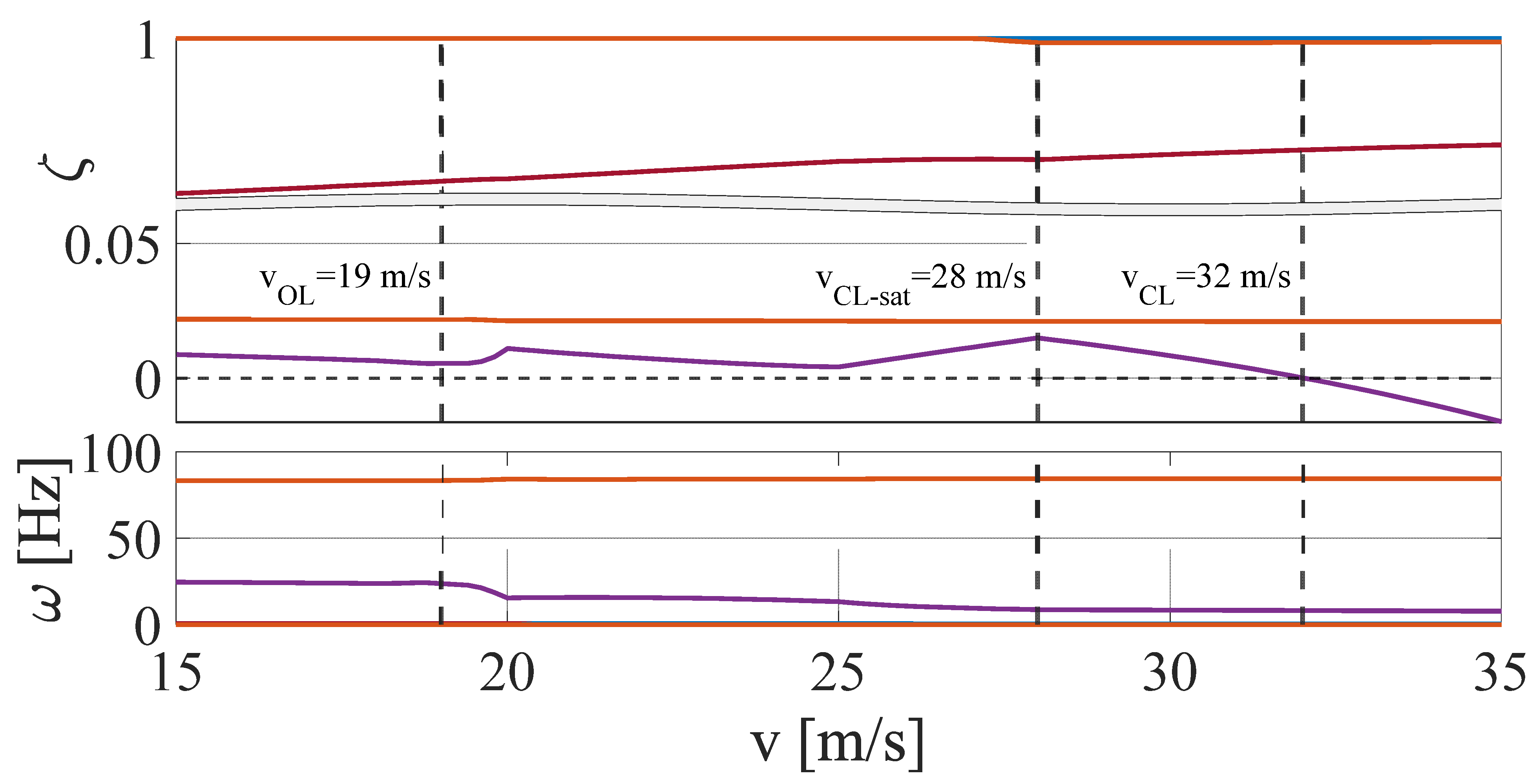
Section 5, the open loop analysis of the system for the identification of the flutter boundary is first carried out. Then, the validation of the static and dynamic behavior of the actuator is done. Moreover, the convergence results of the P D S O optimization procedure are also shown. At last, the comparison between open-loop and closed-loop responses is presented, and some critical situations are simulated in order to study the performance of the closed-loop system.

2. 3DOF Airfoil Model

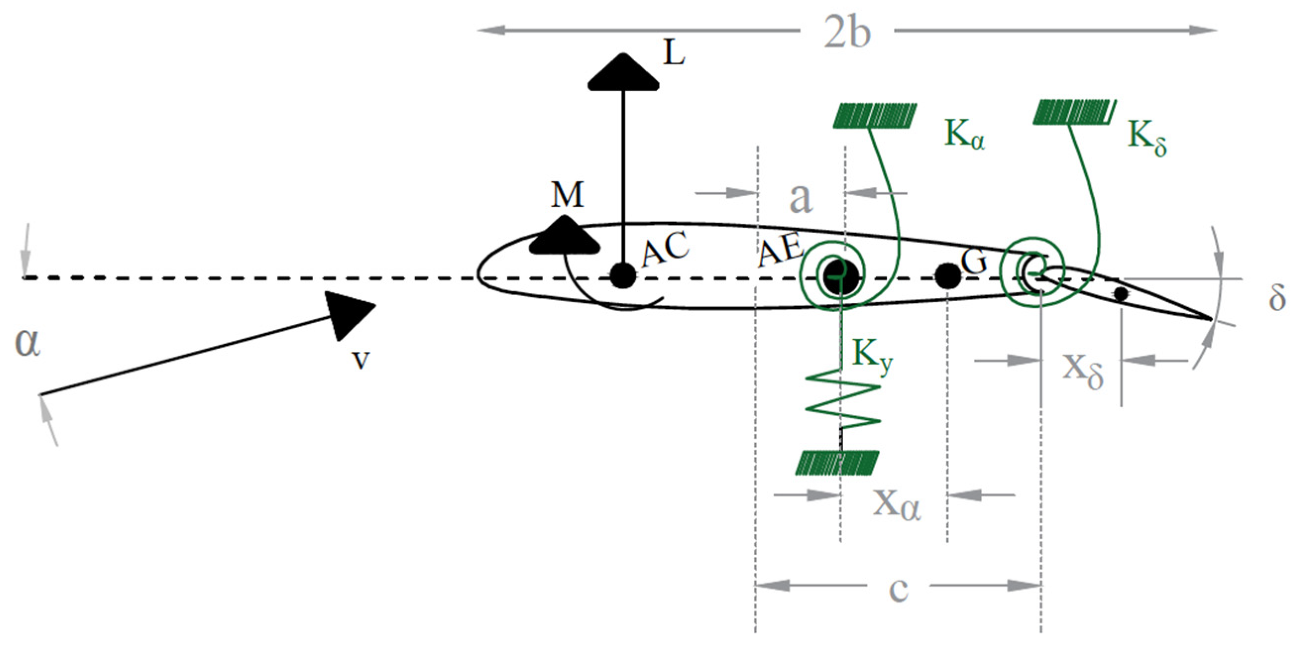
In order to study the flutter phenomenon, a simplification was introduced by reducing the wing to its representative mean airfoil and, as a consequence, a two-dimensional structural model could be considered. The torsional deformability of the wing, which was considered as a beam with a thin-walled section, was simulated by a spring of stiffness K α placed in the axis of elasticity (AE), which represented the constraint. The flexional stiffness was simulated by the heave spring K y . Due to the presence of the flap a third spring of stiffness, K δ was introduced in order to take into account the hinge behavior. In this way the three-degrees-of-freedom concentrated parameters model of the wing, shown in Figure 1, was obtained. Of course, this model had to be considered as a first approximation of the structure, useful for the preliminary studies carried out in this work.
In order to obtain the equations of motion of the three-degrees-of-freedom (3DOF) airfoil, the balance between the inertial, elastic and aerodynamic forces was imposed, writing the system in Equation (1) [24]. The nonlinear stiffness term K α 3 was also considered in order to take into account that nonlinear effects could arise for large displacements, introducing the limit cycle oscillation phenomenon:
{ I α α ¨ + [ I δ + b ( c a ) S δ ] δ ¨ + S α y ¨ + K α α + K α 3 α 3 = M [ I δ + b ( c a ) S δ ] α ¨ + I δ δ ¨ + S δ y ¨ + K δ δ = M S α α ¨ + S δ δ ¨ + m t o t y ¨ + K y y = L
where α and δ are the pitch and flap rotation angles, respectively, while y is the plunge displacement, I α and I δ are the inertia moments, S α and S δ are the static moments, m t o t is the total mass of the wing and the support blocks, L is the lift force and M and M are the aerodynamic moments acting on the airfoil and on the flap, respectively.
In order to carry out the stability analysis of the airfoil, it could be useful to take into account the nondimensional equations of motion. Thus, the first and the second equations of the system in (1) were divided by the term m b 2 , while the third equation was divided by the term m b , obtaining the following system:
{ r α 2 α ¨ + [ r δ 2 + ( c a ) x δ ] δ ¨ + x α y ¨ + r α 2 ω α 2 α ( 1 + γ α 2 ) = M m b 2 [ r δ 2 + ( c a ) x δ ] α ¨ + r δ 2 δ ¨ + x δ y ¨ + r δ 2 ω δ 2 = M m b 2 x α α ¨ + x δ δ ¨ + m t o t m y ¨ + ω y 2 y = L m b
where ω α and ω δ , ω y are the uncoupled natural frequencies, r α and r δ are the gyration radius divided by the semi-chord of the airfoil b and γ is the nonlinear stiffness coefficient, such that K α 3 = γ K α .
In order to obtain the state space model of the system, it was convenient to write the system in matrix form at first (see Equation (3)). The generalized displacement vector X = [ α δ y ] T , the generalized force vector F and the matrices M s and K s , namely the generalized inertia matrix and the stiffness matrix that are reported in Appendix A, were defined:
M s X ¨ + K s X = F
In order to introduce the structural damping contribution, the procedure described by Liu and Dowell [25] was followed, and the damping factors obtained experimentally were treated in the numerical model as modal damping factors. The structural damping matrix was written as
B s = ( Λ T ) 1 B m o d Λ 1
where Λ is the modal matrix, while the modal damping matrix was defined as
B m o d = [ 2 m 1 ω 1 ζ 1 0 0 0 2 m 2 ω 2 ζ 2 0 0 0 2 m 3 ω 3 ζ 3 ]
where m i , ω i and ζ i are the modal masses, the coupled natural frequencies and the measured damping ratios, respectively.
Once the matrices were defined, the model could be written as
M s X ¨ + B s X ˙ + K s X = F
Before defining the state space representation of the analyzed problem, the aerodynamic force model must be introduced.

2.1. Aerodynamic Model

The aerodynamic model considered in this work was the one formulated by Theodorsen [26] for an oscillating airfoil. It was based on the potential flow theory and on the hypothesis that the amplitude of the oscillations is so small that they can be treated as perturbations. According to this theory, the aerodynamic force and moments are functions of the Lagrangian parameters and of the Theodorsen constants T i , reported in Appendix B. The aerodynamic loads were written as follows:
L = ρ b 2 ( v π α ˙ + π y ¨ π b a α ¨ v T 4 δ ˙ T 1 b δ ¨ ) 2 π ρ v b C ( K ) ( v α + y ˙ + b ( 1 2 a ) α ˙ + T 10 v δ π + b T 11 δ ˙ 2 π )
M = ρ b 2 { π ( 1 2 a ) v b α ˙ + π b 2 ( 1 8 + a 2 ) α ¨ + ( T 4 + T 10 ) v 2 δ [ T 1 T 8 ( c a ) T 4 + T 11 2 ] v b δ ˙ [ T 7 + ( c a ) T 1 ] b 2 δ ¨ a π b y ¨ } + 2 π ρ v b 2 ( 1 2 + a ) C ( K ) ( v α + y ˙ + b ( 1 2 a ) α ˙ + T 10 v δ π + b T 11 δ ˙ 2 π )
M = ρ b 2 { [ 2 T 9 T 1 + T 4 ( a 1 2 ) ] v b α ˙ + 2 T 13 b 2 α ¨ + v 2 ( T 5 T 4 T 10 ) δ π v b T 4 T 11 δ ˙ 2 π T 3 b 2 δ ¨ π T 1 b y ¨ } ρ v b 2 T 12 C ( K ) ( v α + y ˙ + b ( 1 2 a ) α ˙ + T 10 v δ π + b T 11 δ ˙ 2 π )
where it appears that the Theodorsen function of the reduced frequency K = b ω v , where v is the airstream velocity and ω is the frequency of the motion. The Theodorsen function was defined as a function of the Hankel function of the second kind as follows:
C ( K ) = H 1 ( 2 ) ( K ) H 1 ( 2 ) ( K ) + i H 0 ( 2 ) ( K )
The structural and aerodynamic formulation discussed is suitable for the analysis of the system in the frequency domain, from which information about the flutter boundary can be obtained. For the aim of this work, it was convenient to introduce time domain analysis. The Duhamel formulation [27] that allows for modeling the arbitrary motion of the airfoil instead of the simple harmonic one was thus introduced by writing the circulatory contribution to the aerodynamic loads as follows:
L c = C ( K ) U ( t ) = U ( 0 ) ϕ ( τ ) + 0 τ U ( σ ) σ ϕ ( τ σ ) d σ
where U ( t ) = v α + y ˙ + b ( 1 2 a ) α ˙ + T 10 v δ π + b T 11 δ ˙ 2 π and ϕ ( τ ) c 0 c 1 e c 2 τ c 3 e c 4 τ have values c 1 = 0.165 , c 2 = 0.0455 , c 3 = 0.335 and c 4 = 0.3 [27].
By integrating parts of Equation (11), a simplified expression of L c was obtained:
L c = U ( τ ) ϕ ( 0 ) + 0 τ U ( σ ) ϕ ( τ σ ) σ d σ
In addition, using the Padè approximation, it could be written as a second-order differential equation, where the two aerodynamic augmented states x ¯ and x ¯ ˙ appear (see Equation (13)):
L c = ( c 0 c 1 c 3 ) U ( t ) + c 2 c 4 ( c 1 + c 3 ) x ¯ + ( c 1 c 2 + c 3 c 4 ) x ¯ ˙

2.2. Augmented State Space Form

The numerical model of the 3DOF airfoil belongs to the class of parameter varying systems, as it depends on the velocity of the airstream. Considering a fixed speed value, the 3DOF model could be considered as a time-invariant system, and thus the augmented state space formulation could be used for the time domain tuning of the controller, introducing the state vector x T = [ α δ y / b α ˙ δ ˙ y ˙ / b x ¯ x ¯ ˙ ] and writing Equations (6)–(9) in matrix form:
M x ˙ = N x + T u + ( x )
Then, the dynamic matrix A = M 1 N was computed. The state input matrix B was defined, taking into account that the input was the flap deflection u = δ c . Thus, B was a column matrix equal to the second column of the dynamic matrix. Lastly, the output state matrix C was imposed to be the identity matrix in the hypothesis of ideal sensors for all the variables. The augmented state space model is written as follows:
{ x ˙ = A x + B u + F ( x ) y = C x
where the term ( x ) = M 1 ( x ) takes into account the nonlinear stiffness contribution.
All the matrices are reported in Appendix A.

3. V-Stack Piezoelectric Actuator

In order to actuate the trailing edge flap for the flutter suppression of the airfoil, the V-stack piezoelectric actuator shown in Figure 2 was chosen [10]. The actuator worked by amplifying the piezoelectric stacks’ deformation induced by an electric voltage. In fact, the two stacks were mounted in a V configuration, and this made the actuator easily installable inside a typical wing structure. By imposing an input voltage, one stack stretched while the other contracted, producing a vertical displacement of the actuator’s tip. The vertical displacement was then transformed in a rotation of the flap through a slider [10].
The piezoelectric stacks were made by overlapping a number n of piezoelectric elements with alternate poling, having alternate positive and negative electrodes printed on the external surfaces. When an electric voltage was imposed, the stacks stretched or contracted along their axes, while the other deformations were negligible. The linear electro-mechanical problem can be expressed by the equation system given by ANSI/IEEE Standard 175-1987 (i.e., the strain charge form), written as follows:
{ ε = S σ + d T E D = d σ + ϵ T E
where ε is the strain, σ is the stress, S is the compliance matrix, d is the piezoelectric matrix, E is the electric field, D is the electric displacement and ϵ is the dielectric constant.

3.1. FEM Model

3.1.1. Piezoelectric Stack Finite Element Model

Taking into account the particular functioning of the piezoelectric stack, Equation (16) can be reduced to the equilibrium equation along the poling direction 3 and, considering the ith piezoelectric layer, it can be written as
ε 33 i = S 33 i σ i 33 + d 33 i E
Then, in the hypothesis that every layer has the same thickness t , compliance S 33 and piezoelectric behavior d 33 , the total stack strain is
ε 33 T = Δ L L = ε 33 i t L = n t L ( S 33   σ 33 + d 33 Δ V t )
where L is the length of the stack and Δ V is the electric voltage imposed. Since n t = L from Equation (18), the stress can be gained:
σ 33 = ε 33 T S 33 d 33 S 33 t Δ V
In order to obtain the element stiffness matrix and the equivalent nodal piezoelectric force vector, the virtual work principle was introduced and, under the hypothesis of absence of external forces, it is written as
L * = ε T σ d Ω = 0
where d Ω is the infinitesimal volume. Substituting Equation (19) into Equation (20) and taking into account that the strain ε and nodal displacement δ are related (i.e., ε = B δ , where B is the finite element strain displacement matrix obtained by deriving the shape function matrix with respect to the space variable), the virtual work can be expressed as
L * = B T 1 S 33 L B d A d L   δ B T d 33 S 33 t Δ V d A d L = 0
where A is the section of the stack.
Due to the particular operating behavior of the stack, the axial behavior was first considered. Substituting into Equation (21) the B matrix of the linear rod finite element, B = 1 L [ 1 1 ] , the equilibrium equation along the axial direction was obtained:
E A L [ 1 1 1 1 ] δ = [ d 33 E A t d 33 E A t ] Δ V
Thus, the element stiffness matrix k ˜ e = E A L [ 1 1 1 1 ] and the equivalent piezoelectric stack nodal force vector F ˜ Δ V = [ d 33 E A t d 33 E A t ] Δ V were defined.

3.1.2. Actuator Finite Element Model

In order to obtain the finite element model of the actuator, the simplified structural scheme shown in Figure 3a was considered, and the mesh shown in Figure 3b was introduced. With the aim of taking into account the presence of the internal hinges of the actuator, four elements of very small lengths and moments of inertia were introduced close to points 3 and 4. In this way, equilibrium was maintained while the flexional stiffness was reduced.
Each finite element of the mesh was a beam and had three degrees of freedom for each node that could be collected in the vector δ T = [ δ i x δ i y φ i δ j x δ j y φ j ] , with i and j being the nodes of the beam while x and y are the local reference system variables along, and normal to, the beam axis oriented from i to j. The element stiffness matrix was the one computed from the Euler–Bernoulli beam. The stacks’ equivalent nodal force vector was obtained, extending the one computed for the piezoelectric rod:
F ˜ Δ V = [ d 33 E A t 0 0 d 33 E A t 0 0 ] T Δ V
In order to obtain the structural discretized model, a coordinate transformation from the local to the global reference frame was introduced, and the structural stiffness matrix was computed.
The structural nodal force vector is defined as follows:
[ F 3 X F 3 Y F 4 X F 4 Y ] = [ E s t a c k ( 1 3 ) A s t a c k ( 1 3 ) d 33 ( 1 3 ) cos θ ( 1 3 ) t ( 1 3 ) E s t a c k ( 1 3 ) A s t a c k ( 1 3 ) d 33 ( 1 3 ) sen θ ( 1 3 ) t ( 1 3 ) E s t a c k ( 2 4 ) A s t a c k ( 2 4 ) d 33 ( 2 4 ) cos θ ( 2 4 ) t ( 2 4 ) E s t a c k ( 2 4 ) A s t a c k ( 2 4 ) d 33 ( 2 4 ) sen θ ( 2 4 ) t ( 2 4 ) ] Δ V
where d 33 ( 2 4 ) = d 33 ( 1 3 ) , since the piezoelectric stacks work anti-symmetrically, and θ is the angle between the global X and the beam local x axes.
The finite element model K S T δ = F was obtained and, by imposing the boundary conditions, the static behavior of the actuator could be studied, resolving the system:
{ K 11 δ u + K 12 δ k = F k K 12 T δ u + K 22 δ k = F u
where the subscripts u and k stand for unknown and known, respectively.
As the study of the dynamic behavior of the actuator was in the aim of this work, the equations of motion of the structure were written. Thus, the consistent mass matrix of the beam was introduced:
m ˜ e = ρ A l 420 [ 140 0 0 70 0 0 0 156 22 l 0 54 13 l 0 22 l 4 l 2 0 13 l 3 l 2 70 0 0 140 0 0 0 54 13 l 0 156 22 l 0 13 l 3 l 2 0 22 l 4 l 2 ]
With this, the structural mass matrix M S T was computed.
The structure equations of motion were written in line with the findings of Paz and Kim [28]:
M S T δ ¨ + K S T δ = F
In order to take into account the structural damping contribution, the damping matrix was computed. For the piezo stacks’ damping contribution, the dielectric loss factor tan δ was taken into account as it is related to the quality factor Q by the relation tan δ = 1 Q , and with the damping factor being ζ = 1 2 Q , it could be obtained that [29]
ζ = tan δ 2
The equations of motion of the stacks in the local frame are
m ˜ e δ ˜ ¨ + C ˜ s t a c k δ ˜ ˙ + k ˜ s t a c k δ ˜ = F ˜ Δ V
where m ˜ e , C ˜ s t a c k and k ˜ s t a c k are the mass, damping and stiffness matrices in the local frame, respectively. It can be seen that there was an analogy between Equation (29) and the classic mass-spring-damper equation of motion. Therefore, the following equality can be imposed:
m ˜ e 1 C ˜ s t a c k = 2 ζ ω n
In addition, the damping matrix is computed as
C ˜ s t a c k = tan δ ω n m ˜ e
where ω n is the natural frequency of the actuator modes, though only the first is retained in this work.
The damping of the steel elements of the actuator was instead introduced using the Rayleigh model:
C = a M + b K
where a and b are arbitrary coefficients, computed in this work using a population decline swarm optimization P D S O algorithm, described in Appendix C. The P D S O algorithm was implemented for the identification of the actuator experimental frequency response, presented by [10], choosing as an objective function the percentage error % E M r between the experimental resonance peak M r = 3.95 × 10 2 m m V and the one computed from the finite element model. The optimization problem is written as
min % E M r s . t . a m i n a a m a x b m i n b b m a x
Each particle had two coordinates P λ i = [ a i b i ] λ that could assume only the values inside the research space ( 1 E 5 a 1 E 3 , 1 E 5 b 1 E 3 ). The research space limits were chosen by a trial and error approach, looking for minimization of the percentage error. The algorithm parameters were chosen as follows: c c = c s = 2.025 , μ m i n = 0.4 , μ m a x = 0.9 , Λ = 40 , ζ = 0.5 and Δ = 10 . The minimum value of the objective function min % E M r = 0.0055 % was already obtained for an initial maximum number of particles equal to 20, and the minimum point had the coordinates a = 1.5 E 4 , b m i n = 1.7 E 5 .
By introducing the damping contribution and imposing the boundary conditions, the equations of motion of the actuator are written as
M 11 δ ¨ u + C 11 δ u ˙ + K 11 δ u = F k
In order to obtain the theoretical frequency response, the transfer function of the actuator was computed. The state space model was introduced, defining the state vector x T = [ δ i δ i ˙ ] and the following matrices:
A = [ 0 ( n x n ) I ( n x n ) M 11 1 K 11 M 11 1 C 11 ] ;   B = [ 0 ( n x 1 ) M 11 1 F n ] ;   D = 0 ( n x 1 ) ;
where n is the degree of freedom of the actuator. The C matrix was defined in such a way that the model returned as an output the vertical displacement of point 6 (i.e., the tip of the actuator). The transfer function is computed as
G v 6 = C ( s I A ) 1 B + D
Lastly, it must be pointed out that to model the internal hinges of the actuator, four finite elements having a length equal to 1% of the membership elements were introduced. The fictitious finite element moments of inertia were obtained by dividing the membership element ones by a factor f, chosen in such a way that the minimum error on the static and dynamic behavior was obtained. For the sake of clarity, looking at Figure 3b, the membership element of the fictitious hinge finite element 10–3 is the finite element 1–10. Figure 4 shows the percentage errors computed between the FE model and the experimental results of the piezoelectric V-stack actuator stroke, namely δ 6 Y , of its blocked force F 6 Y and of the resonance frequency as a function of the fictitious hinge factor f. Looking at Figure 4, it appears that the optimal dividing factor choice was f = 10 6 .

4. Gain-Scheduled Filtered PID Active Controller

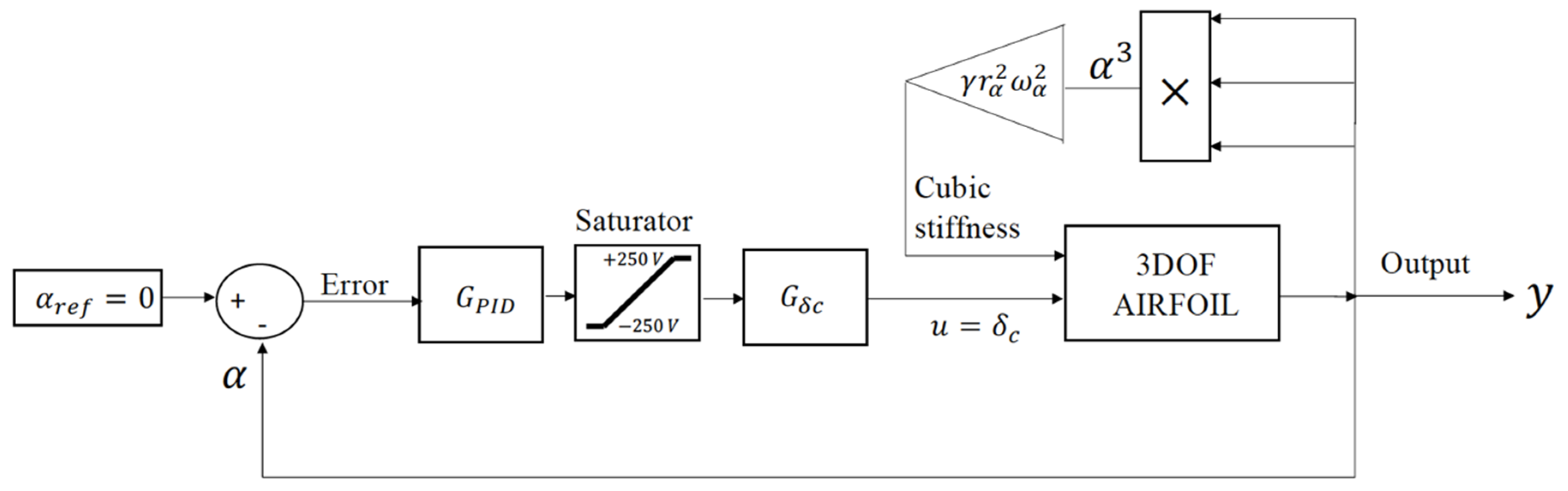
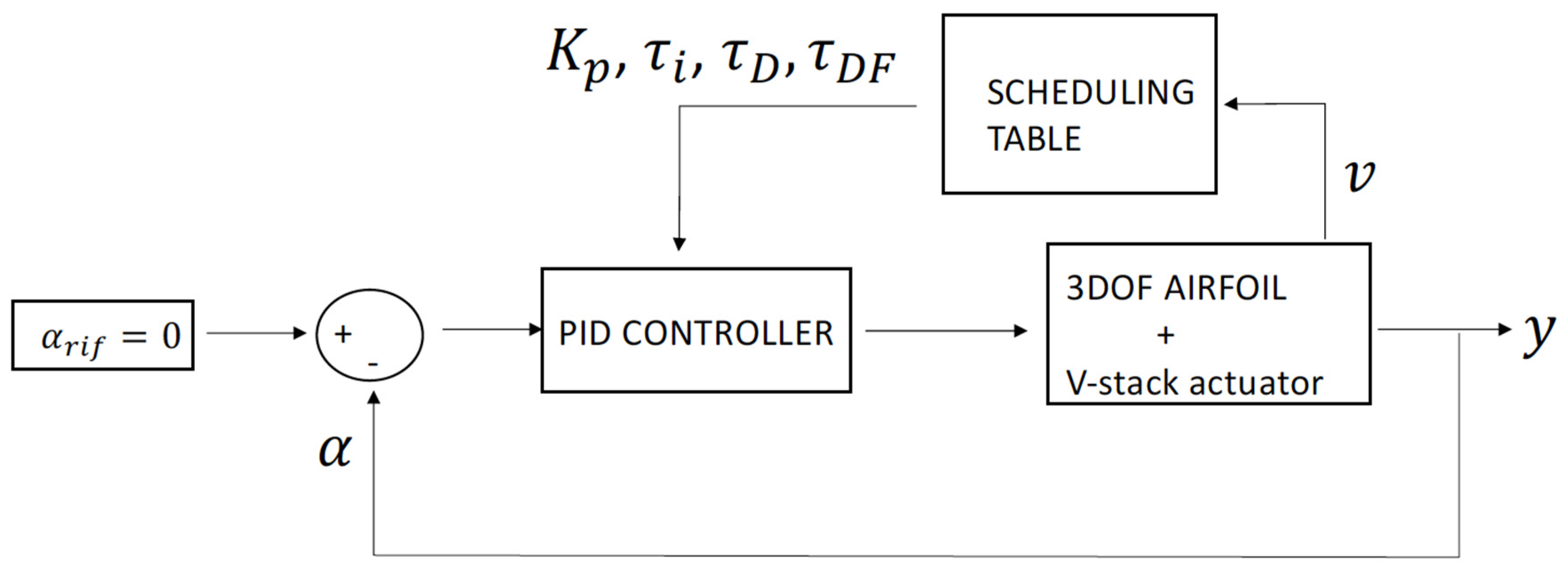
The control architecture chosen in this work and shown in Figure 5 was based on an output feedback scheme based on a filtered Proportional-Integral-Derivative fPID controller that presented some benefits. This type of controller presented a simplicity in implementation and installation and, moreover, it only requested one output measure, thus asking for the implementation of only one sensor device and allowing us to avoid the complication of the controller scheme introduced by, for instance, state observers. These are some of the reasons that currently still motivate the use of PID controllers in the industry [
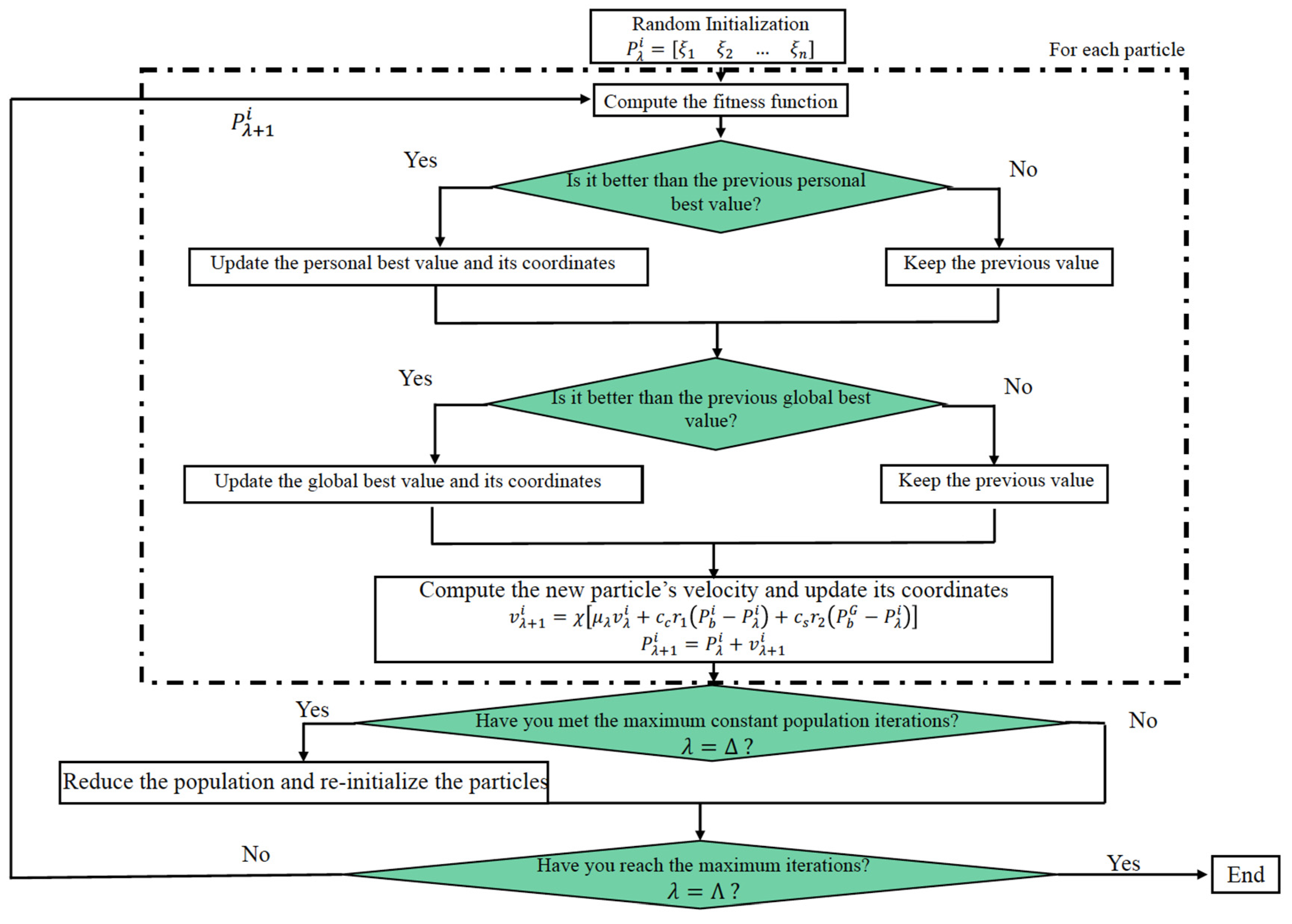
30]. Moreover, the PID controller had a fixed structure, and the problem reduced to the tuning of its parameters, which were made in this work using a population decline swarm optimization P D S O algorithm. The principal issue of choosing a PID controller is that it is not adaptive with the system’s change of parameters. In this work, in order to make the controller adaptive in velocity, a gain scheduling (GS) approach was used.
The filtered PID controller acted by minimizing the error function e ( t ) = α r e f ( t ) α ( t ) , being α r e f ( t ) = 0 r a d , because the aim was to stabilize the system. The reference signal sent to the actuator was the voltage input, and it was computed as the sum of three terms: one proportional to the current error, one proportional to the time integral of the error, ensuring the system reached the desired setpoint, and the last term proportional to the filtered error time derivative [30]:
Δ V ( t ) = K p [ e ( t ) + 1 τ i 0 t e ( τ ) d τ + e D ( t ) ]
where e D ( t ) is the solution of the following first-order differential equation:
τ D F e ˙ D + e D = τ D e ˙
The choice of a controller with all three components was related to the peculiarities of each term. In fact, a proportional-only controller could not make the system able to reach the setpoint. By increasing the proportional gain, the difference between the actual and desired values could be reduced, but the system would encounter more oscillations for the rapid transient; thus, the integral contribution was added. At least, the derivative terms allowed the system to tackle the rapid transient easily, as the derivative gave information on the evolution of the error. Thus, the controller was able to forecast and fill the eventual delays, leading to a reduction of the oscillation amplitude.
The controller parameters, namely K p ,   τ i , τ D and τ D F , had to be tuned in such a way that no instabilities due to the control were introduced, and the flap displacement had to be able to stabilize the airfoil in the shortest time. In order to obtain the PID controller at the flutter speed, a P D S O algorithm was used, and the fitness function to be minimized was chosen to be the integral of time absolute error (ITAE).
It is worth noting that that, strictly speaking, heuristic optimizers did not find the actual optimum, but their solution was always the best parameter configuration among all the other configurations that were tested. This means that the controller might be suboptimal because it is just the best among the tested ones. This is particularly true when a flat region of the performance index is found. Thus, considering that the PID tuning was gained via a numeric metaheuristic approach, the obtained controller was to be considered as a suboptimal one. With regard to the objective function, it should be noted that the ITAE was chosen because it had the ability to highlight the divergence error that occurred when incorrect controller parameters were used and the flutter vibration started increasing slowly. The mathematical expression of the fitness function is the following:
I T A E = t 0 T w | e ( t ) | t d t
where t 0 is the instant of perturbation and T w is the time window chosen for the computation of the function, being large enough to include the entire transient response, but not too much to affect the computational cost of the algorithm. In this study, it was imposed to be t 0 = 0 s and T w = 1 s.
Each particle P i at each iteration λ was defined in the algorithm by four coordinates P λ i = [ K p i τ i i τ D i τ D F i ] λ , and the minimization problem was expressed as follows:
min I T A E ( P λ i ) s . t . l o c a l   s t a b i l i t y K p m i n K p K p m a x τ i m i n τ i τ i m a x τ D m i n τ D τ D m a x τ D F m i n τ D F τ D F m a x
where the research space limits were chosen by a preliminary trial and error approach.
As the speed can vary, the 3DOF airfoil model is a parameter varying system, and for this family of dynamic systems, the simplest method to obtain adaptive controllers is the gain scheduling (GS) method. The GS method was implemented by defining a set of controllers tuned for different working conditions of the system, which were identified by an appropriate scheduling variable, in this case the airstream speed. However, each controller guaranteed the desired performance only locally, and thus an interpolation of the controller parameters had to be introduced [31]. The gain scheduling control architecture used is shown in Figure 6.
In order to compute the scheduling table, the P D S O algorithm was used for different velocity values, and the optimal PID controller for each one was found. A set of linear, time-invariant sub-optimal controller parameters was obtained, and a linear interpolation of the PID parameters was introduced to obtain a parameter-varying controller.

5. Numerical Results

In this section, the numerical results of the aeroelastic model and the FEM actuator model are analyzed. First, the open-loop analysis of the 3DOF airfoil is carried out, and then the validation of the FEM model of the actuator is done. Lastly, some critical case studies for the closed-loop system are analyzed.

5.1. Open-Loop Analysis of the Aeroelastic System

The experimental model considered in this work was the one studied by Ardelean et al. [4] at Duke University, and its parameters are listed in Table 1. In order to study the stability of the airfoil, the eigenvalue problem det ( λ I A ) = 0 was solved, and the root locus, shown in Figure 7, was obtained, varying the airstream velocity. It can be seen that the system had three pairs of complex eigenvalues and a pair of real eigenvalues. Instability was reached when the real part of one complex eigenvalues pair became positive in value.
In order to determine the flutter speed, the damping ratio variation with the airstream velocity was studied, obtaining the diagram shown in Figure 8, where it can be seen that the damping ratio related to the unstable eigenvalue became negative in value for a speed equal to v f l u t t e r = 19 m s while the flutter frequency was ω f l u t t e r = 4.2   Hz . These results are in accordance with the ones presented by Ardelean et al. [32].
When the flutter speed was exceeded, the limit cycle oscillation (LCO) phenomenon arose. Thus, the oscillations presented a growing amplitude with the velocity. In Figure 9, the LCO amplitudes on α with the airstream velocity are shown.

5.2. Actuator Validation

The curves of the tip’s vertical displacement and blocked force versus the electric voltage obtained from Equation (25) were compared with the theoretical ones presented by Ardelean et al. [10]. This is shown in Figure 10, where it can be seen that the FEM and theoretical curves almost overlapped. In fact, errors of 0.15 % for the stroke and 0.055 % for the blocked force were obtained. The actuator’s data are listed in Table 2.
In order to validate the dynamic behavior of the actuator, the bode diagram of the transfer function computed in Equation (35) was compared with the experimental frequency response of the actuator presented by Ardelean et al. [10]. From Figure 11, it can be seen that in the bandwidth region extending up to 200 Hz, the two curves overlapped, while some differences appeared beyond the first natural frequency of the actuator. These differences were due to the actuator’s parameters’ uncertainty and the difference between the theorical and real values of the materials’ constants. However, it is worth noting that such a discrepancy would not affect the closed-loop system, while the flutter frequency of the airfoil fell in the bandwidth region. Therefore, the FEM model was acceptable for the frequency range of interest.

5.3. GS-fPID Controller Tuning

The minimization problem defined in Equation (39) was solved using the P D S O algorithm. First of all, the research space limits were defined as 0.10 V d e g K p 2 E 4 V d e g , 1   s τ i 1 E 4   s , 1 E 4   s τ D 1   s e 1 E 4   s τ D F 3   s . For a larger research space, a higher number of particles was needed to achieve the convergence and the computational cost of the procedure’s increases. The algorithm parameters were chosen as was done before for the damping contribution in the FEM model of the actuator, and four optimizations were done with different maximum numbers of particles P m a x = [ 5 10 20 50 ] in order to study the convergence of the procedure. For each optimization, the algorithm was run 10 times, and the final values of the objective function were analyzed to compute the minimum, maximum, median and standard deviation. These convergence indexes are shown in Table 1, while in Figure 12, the ITAE trends for any initial swarm size are shown.
From the results shown in Table 1, it can be seen that the minimum objective function value was I T A E m i n = 4.51 E 5 r a d s , and it was already obtained for a maximum number of particles P m a x = 20 . The coordinates of the point of minimum were K p = 7.8 E 3 V d e g ; τ i = 1 E 4 s; τ D = 0.255 s; τ D F = 1 s. The values of the time constants were the same for each initial swarm size, so they are not reported in Table 3. It can be seen that, by increasing the initial swarm size, the possibility to lock into local minima reduced (see Figure 12), and the values of the convergence indexes reduced because of the higher research capability. However, the CPU time increased, as expected.
In order to tune the gain scheduling adaptive controller, the P D S O algorithm was used for each speed value of the vector v = [ 15 18 18.5 19.5 20 25 28 ] , obtaining the scheduling table reported in Table 4. From the results reported in Table 4, it can be seen that in the speed range higher than 19 m/s, τi assumed the research space upper limit value. It has been noted that, by increasing the upper limit, τi tended to always assume its higher value, while the other parameters remained unchanged. This behavior indicates that, in such a range of velocities, the integral contribution to the controller was negligible when compared with the proportional and derivative ones. Thus, the heuristic tuning procedure suggests that a PD scheme would be more suitable in such speed range. Moreover, looking at Table 4, it can also be noted that τD and τDF reached, in some cases, the limiting values of their research spaces. By carrying out numerical tests, it was noted that if a wider research space was selected for τD and τDF, several pairs of τD and τDF values would give the same minimum value of the objective function. This indicates a flat region of the objective function with respect to these variables.
Moreover, regarding the tendencies of the obtained scheduling values, it must be noted that the heuristic approaches were useful because they allowed for finding good solutions despite the complexity of the objective function. Moreover, they also allowed for finding a good solution even when the shape of the objective function was not known. This was the case when a performance index, such as the ITAE, was selected as an objective function. The physical meaning of the performance index must, of course, be clear, but its behavior with respect to both the tuning parameters (such as the PID gains in the present work) and the system’s parameters (such the velocity) is generally unknown or hard to obtain analytically (particularly when nonlinearities are also present). The metaheuristic algorithms allow for treating such optimization problems in an easy way, but to know the reason why some solutions are obtained using the metaheuristic optimization is hard, and this is what it takes. The designer just has to ensure that the obtained solution is meaningful from physical and technological points of view. In particular, one of the points to be addressed is the stability of the controlled plant. In this work, by means of an engineering approach, it was verified by carrying out numerical simulations of the nonlinear closed-loop system and looking for PID parameter sets that ensure the local linearized plant stability (aware of the fact that the local stability may not be straightforward in ensuring the stability of the time-varying systems that can ask for ad hoc adaptive approaches).
Figure 13 shows the damping ratio and the natural frequencies of the closed-loop system as a function of the advancing velocity. The modes associated with the structural V-stack mechanism were omitted for the sake of clarity of the diagram. In particular, when looking at the closed-loop modal damping ratio trend, it can be seen that a pair of conjugate poles became unstable for velocities higher than 32 m s . It is worth noting that to obtain the modal characteristics shown in Figure 13, the closed-loop system was linearized. However, when the actuator saturation was taken into account, the controller was no longer able to stabilize the system for speed values higher than 28 m s , as will be shown in the next numerical studies. Thus, the flutter boundary of the closed loop system was 28 m s .
In Figure 14, the pole map of the PID transfer function is shown. The PID transfer function had two poles; one pole was always equal to zero, while the other changed with the airstream velocity, according to the change of the PID parameters. In fact, starting from a speed of 15 m s , the normalized frequency of the real non-zero pole assumed a value of ω n = 0.074   Hz , and when the open-loop flutter boundary was reached, it assumed the value ω n = 0.159   Hz , which was maintained until a speed of 25 m s . This stemmed from the absence of poles that were too fast, allowing its implementation into a flight computer which could have a sampling of 5 ms (see, for instance, Waitman and Marcos [20]).

5.4. Closed-Loop Analysis

The PID parameters obtained from the optimization done in Section 5.3 were then used to run a simulation of the closed-loop system at the flutter speed. The initial state vector for the simulation was x 0 T = [ 0.05 0.025 0 0 0 0 0 0 ] , and the responses shown in Figure 15 were obtained. It can be seen that the system was able to suppress the flutter oscillations on α in less than 0.1 seconds without any overshoot, while for the plunge displacement and the flap deflection, the maximum values were y m a x = 0.0011   m and δ m a x = 14.9 ° , respectively.
As in the first case study for the closed-loop system with a gain-scheduling adaptive controller, a linear variation of the speed, starting from 15 m s and with a 2 m s 2 slope, was considered, and the responses shown in Figure 16 and Figure 17 were obtained. It can be seen that the initial perturbation was rapidly suppressed, as clearly shown in Figure 17, where the time window was limited to one second of analysis. Then, at the time instant t = 2   s , the flutter boundary of the open-loop system was reached. Thus, it started oscillating, with increasing LCOs as the speed increased. On the other hand, the closed-loop system did not show oscillations until the time instant t = 6.5   s , when flap-unstable oscillations arose, suggesting that the closed-loop flutter boundary was exceeded. Looking at the velocity diagram in Figure 16, the closed loop-flutter boundary is represented by the speed of 28 m s , as previously stated. It can be said that the adaptive controller was able to stabilize the system in the new flight envelope assigned.
Looking at Figure 8, it can be noted that the instability arose after an abrupt variation of the damping ratio, starting from the velocity value v = 15 m s . Thus, it was useful to study the controller performance in such a critical speed range. The controller stress case was chosen to be a speed ramp from 15 m s to 28 m s with different acceleration values, while a constant disturbance on the flap deflection equal to 5 ° occurred. From the responses shown in Figure 18, it can be seen that the transient response was almost equal for all the accelerations studied, and the unstable oscillations that occurred after reaching the closed-loop flutter boundary had the same amplitudes. Therefore, the controller reaction was considered good for both the considered velocity variation and the disturbance.
As in the last closed loop case study, a sinusoidal velocity variation within the range v [ 15 m s 28 m s ] was imposed, while a random disturbance on the flap deflection δ d [ 5 ° 5 ° ] occurred. From the responses shown in Figure 19, it can be seen that the controller was able to face up to the simultaneous variation of speed and the disturbances, avoiding instability conditions and maintaining the state variable peaks at acceptable values from a mechanical point of view. In fact, it can be seen that during the transient response, the rotation of the airfoil assumed the maximum value α m a x = 1.1 ° , the flap deflection was limited to δ m a x = 15 ° , and the plunge displacement presented a pick equal to y m a x = 10 3 m . In addition, all three responses were stabilized to the equilibrium point in almost 0.7 seconds, presenting slight fluctuations due to the presence of the disturbance.

6. Conclusions

In this paper, the numerical model of a three-degrees-of-freedom airfoil was studied in order to predict the flutter boundary of the system. With the aim of taking into account the piezoelectric V-stack actuator, a finite element model was introduced. The validation of the static and dynamic behavior of the actuator with the experimental data given in the literature was carried out. A heuristic swarm method named P D S O was employed for the tuning of a gain-scheduling adaptive controller based on a filtered PID controller. An increase of the flutter boundary of the system of about 47% was obtained. Lastly, in order to study the performance of the closed-loop system, several simulations were carried out, considering critical values of acceleration and speed and taking into account the presence of disturbances. The actuator FEM model computed in this work can represent a starting point for the study of the influence of materials and geometric configurations in the V-stack actuator flutter suppression capability. Moreover, the airfoil flutter suppression PDSO tuning approach presented in this work could be used, for instance, as a reference approach for a less simple model or hardware in the loop control tuning of an aerodynamic surface, using the local sensors’ output time histories to define the objective function to be minimized.

Author Contributions

Conceptualization, C.O. and A.M.; Data curation, C.R.V.; Methodology, C.O. and A.M.; Software, C.R.V.; Supervision, A.M.; Writing—original draft, C.R.V.; Writing—review & editing, C.O. All authors have read and agreed to the published version of the manuscript.

Funding

This research received no external funding.

Institutional Review Board Statement

Not applicable.

Informed Consent Statement

Not applicable.

Data Availability Statement

Not applicable.

Conflicts of Interest

The authors declare no conflict of interest.

Appendix A

3DOF Airfoil Matrices

In accordance with Li et al. [27], the matrices of the 3DOF airfoil structural model reported here.
For the nondimensional equations of motion from Equation (3), the following matrices are defined:
M s = [ r α 2 r δ 2 + ( c a ) x δ x α r δ 2 + ( c a ) x δ r δ 2 x δ x α x δ m t o t m ] K s = [ r α 2 ω α 2 0 0 0 r δ 2 ω δ 2 0 0 0 ω y 2 ]
For the state space model in Equation (15), the following matrices are defined, where the subscripts s and n c stand for structural and non-circulatory, respectively:
M n c = ρ m [ π b 2 ( 1 8 + a 2 ) [ T 7 + ( c a ) T 1 ] b 2 π a b 2 2 T 13 b 2 T 3 b 2 π T 1 b 2 π a b 2 T 1 b 2 π b 2 ] K n c = ρ m [ 0 ( T 4 + T 10 ) v 2 0 0 ( T 5 T 4 T 10 ) v 2 π 0 0 0 0 ] B n c = ρ m [ π ( 1 2 a ) v b [ T 1 T 8 ( c a ) T 4 + T 11 2 ] v b 0 [ 2 T 9 T 1 + T 4 ( a 1 2 ) ] v b T 4 T 11 v b 2 π 0 π v b v T 4 b 0 ] R T = [ 2 π ρ v ( a + 1 2 ) m ρ v T 12 m 2 π ρ v m ] S 1 = [ v T 10 v π 0 ] S 2 = [ b ( 1 2 a ) b T 11 2 π b ] S 3 = [ c 2 c 4 ( c 1 + c 3 ) v b ( c 1 c 2 + c 3 c 4 ) v ] M t = M s M n c K = K s K n c 1 2 R S 1 B = B s B n c 1 2 R S 2 D = R S 3 E 1 = [ 0 0 0 v b v T 10 π b 0 ] E 2 = [ 0 0 0 ( 1 2 a ) T 11 2 π 1 ] E 3 = [ 0 1 c 2 c 4 ( v 2 b ) ( c 2 + c 4 ) v b ] M = [ I 0 0 0 M t 0 0 0 I ] N = [ 0 I 0 K B D E 1 E 2 E 3 ]

Appendix B

Theodorsen Constants

The constants T i that appear in the aerodynamic load expressions in Equations (7)–(9) are reported here in accordance with NACA report n.496 [26]:
T 1 = c arccos ( c ) 1 3 ( 2 + c 2 ) 1 c 2 T 2 = c ( 1 c 2 ) ( 1 + c 2 ) 1 c 2 arccos ( c ) + c 2 arccos 2 ( c ) T 3 = 1 4 c ( 7 + 2 c 2 ) 1 c 2 arccos ( c ) ( 1 8 + c 2 ) arccos 2 ( c ) 1 8 ( 1 c 2 ) ( 5 c 2 + 4 ) T 4 = c 1 c 2 arccos ( c ) T 5 = 2 c 1 c 2 arccos ( c ) arccos 2 ( c ) + c 2 1 T 6 = T 2 T 7 = 1 8 c ( 2 c 2 + 7 ) 1 c 2 ( 1 8 + c 2 ) arccos ( c ) T 8 = c arccos ( c ) 1 3 ( 2 c 2 + 1 ) 1 c 2 T 9 = 1 2 [ 1 3 ( 1 c 2 ) 3 + a T 4 ] T 10 = 1 c 2 + arccos ( c ) T 11 = ( 1 2 c ) arccos ( c ) + ( 2 c ) 1 c 2 T 12 = ( 2 + c ) 1 c 2 ( 2 c + 1 ) arccos ( c ) T 13 = 1 2 [ T 7 + ( c a ) T 1 ]

Appendix C

Population Decline Swarm Optimization: P D S O

The P D S O is a variant of particle swarm optimization (PSO). It is a stochastic optimization procedure based on a social model for which a swarm of particles is defined, and for each one, a set of variables is assigned. The aim of the algorithm is to find the values of the parameters associated with the minimum point of the objective function [30]. At the first iteration step, a set of coordinates inside the research space are defined, and a set of random directional velocity values are assigned to each particle. Then, the objective function is computed for each particle and it is assigned as an individual best value, while the minimum objective function value among all the particles is searched for to define the global minimum. At the end of the iteration, the new coordinates and velocities of the particles are computed in order to make them follow the best solution. During successive iterations, it is verified that the new coordinates fall in the research space defined, and the individual and global best solutions are updated. The algorithm stops when a convergence condition is achieved or when the maximum iterations Λ are reached. The flowchart of the algorithm is shown in Figure A1.
The P D S O is a PSO algorithm, where the reduction of the number of particles is considered during its evolution. In fact, a decline factor ζ < 1 is defined, and when a certain number of iterations Δ is reached, the population is reduced ( P = ζ P m a x ). While a higher maximum number of particles is related to greater research capability and a lower probability of the local minimum lock problem, it leads to a higher computational cost of the procedure. A proper setting of parameters allows for a best compromise between the initial global search capability and final faster exploitation ability of the swarm. A reinitialization of some particle coordinates and velocities can be introduced together with the population reduction. In this way, new trajectories of the particles are explored, reducing the local minimum lock events.
The mathematical formulation of the algorithm is explained in the following. First of all, a number n of parameters ξ is assigned to each particle.
Figure A1. P D S O flowchart.
Vibration 04 00024 g0a1
P λ i = [ ξ 1 ξ 2 ξ n ]
where λ = 1 , 2 , , Λ is the actual iteration step. Thus, after the objective function is computed for each particle, their positions are updated:
P λ + 1 i = P λ i + v λ + 1 i
where v λ + 1 i is the updated velocity, defined as
v λ + 1 i = χ [ μ λ v λ i + c c r 1 ( P b i P λ i ) + c s r 2 ( P b G P λ i ) ]
where c c and c s are the cognitive and social acceleration coefficients, respectively; r 1 and r 2 are random coefficients inside the range [ 0 1 ] ; and μ λ is the inertia factor introduced to balance the local and global searches, varying linearly with the iterations according to the following relation:
μ λ = μ m a x ( 1 λ Λ ) + μ m i n λ Λ
At last, χ is the constriction factor introduced to avoid the explosion of the swarm, computed as
χ = 2 | 2 ϕ ϕ 2 4 ϕ
where ϕ = c c + c s > 4 is imposed in order to ensure the stability of the algorithm [33].
The population reduction model is defined as suggested by Orlando and Alaimo [30]:
P λ = { P m a x    s e λ = 1 P λ ζ    s e λ Δ = λ Δ P λ 1    o t h e r w i s e
where the notation x stands for the integer part of x , such that x = x .

References

  1. Jonsson, E.; Riso, C.; Lupp, C.A.; Cesnik, C.E.; Martins, J.R.; Epureanu, B.I. Flutter and post-flutter constraints in aircraft design optimization, Prog. Aerosp. Sci. 2019, 109, 100537. [Google Scholar]
  2. Landa, P.S.; Strelkov, S.P.; Yakovleva, M.V. Bending-torsional flutter of an airfoil with balance mass. Radiophys. Quantum Electron. 1968, 11, 628–632. [Google Scholar] [CrossRef]
  3. Giurgiutiu, V. Review of smart-materials actuation solutions for aeroelastic and vibration control. J. Intell. Mater. Syst. Struct. 2000, 11, 525–544. [Google Scholar] [CrossRef]
  4. Walz, C.; Chopra, I. Design and testing of a helicopter rotor model with smart trailing edge flaps. AIAA meeting paper. In Proceedings of the Adaptive Structures Forum, Hilton Head, SC, USA, 21–22 April 1994; p. 1767. [Google Scholar]
  5. Heeg, J. Analytical and Experimental Investigation of Flutter Suppression by Piezoelectric Actuation; National Aeronautics and Space Administration, Office of Management, Scientific and Technical Information Program: Washington, DC, USA, 1993.
  6. Lazarus, K.B.; Crawley, E.F.; Bohlmann, J.D. Static aeroelastic control using strain actuated adaptive structures. J. Intell. Mater. Syst. Struct. 1991, 2, 386–410. [Google Scholar] [CrossRef]
  7. Fichera, S.; Isnardi, I.; Mottershead, J.E. High-bandwidth morphing actuator for aeroelastic model control. Aerospace 2019, 6, 13. [Google Scholar] [CrossRef] [Green Version]
  8. Han, J.H.; Tani, J.; Qiu, J. Active flutter suppression of a lifting surface using piezoelectric actuation and modern control theory. J. Sound Vib. 2006, 291, 706–722. [Google Scholar] [CrossRef]
  9. Hall, S.R.; Prechtl, E.F. Design of a high efficiency, large stroke, electromechanical actuator. Smart Mater. Struct. 1999, 8, 13. [Google Scholar]
  10. Ardelean, E.V.; Cole, D.G.; Clark, R.L. High Performance ‘‘V-stack’’ Piezoelectric Actuator. J. Intell. Mater. Syst. Struct. 2004, 15, 879–889. [Google Scholar] [CrossRef]
  11. Chen, C.L.; Peng, C.C.; Yau, H.T. High-order sliding mode controller with backstepping design for aeroelastic systems. Commun. Nonlinear Sci. Numer. Simul. 2012, 17, 1813–1823. [Google Scholar] [CrossRef]
  12. Utkin, V.; Poznyak, A.; Orlov, Y.; Polyakov, A. Conventional and high order sliding mode control. J. Frankl. Inst. 2020, 357, 10244–10261. [Google Scholar] [CrossRef]
  13. Na, S.; Librescu, L.; Kim, M.H.; Jeong, I.J.; Marzocca, P. Robust aeroelastic control of flapped wing systems using a sliding mode observer. Aerosp. Sci. Technol. 2006, 10, 120–126. [Google Scholar] [CrossRef]
  14. Yang, P.; Li, Q.D.; Ren, Z.; Tan, Q.K.; Fan, Y. Active control method on flutter suppression of a high-aspect-ratio two-dimensional airfoil with a control surface. In Proceedings of the 2014 IEEE Chinese Guidance, Navigation and Control Conference, Yantai, China, 8–10 August 2014; p. 2745. [Google Scholar]
  15. Wang, Z.; Behal, A.; Marzocca, P. Model-free control design for multi-input multi-output aeroelastic system subject to external disturbance. J. Guid. Control Dyn. 2011, 34, 446–458. [Google Scholar] [CrossRef]
  16. Zhang, K.; Wang, Z.; Behal, A.; Marzocca, P. A continuous robust control strategy for the active aeroelastic vibration suppression of supersonic lifting surfaces. Int. J. Aeronaut. Space Sci. 2012, 13, 210–220. [Google Scholar] [CrossRef] [Green Version]
  17. Bernelli-Zazzera, F.; Mantegazza, P.; Mazzoni, G.; Rendina, M. Active flutter suppression using recurrent neural networks. J. Guid. Control Dyn. 2000, 23, 1030–1036. [Google Scholar] [CrossRef]
  18. Andrievsky, B.; Kudryashova, E.V.; Kuznetsov, N.V.; Kuznetsova, O.A.; Leonov, G.A. Simple adaptive control for airfoil flutter suppression. Math. Eng. Sci. Aerosp. 2018, 9, 5. [Google Scholar]
  19. Takarics, B.; Vanek, B. Tensor product model-based robust flutter control design for the FLEXOP aircraft. IFAC-PapersOnLine 2019, 52, 134–139. [Google Scholar] [CrossRef]
  20. Waitman, S.; Marcos, A. H∞ Control Design for Active Flutter Suppression of Flexible-Wing Unmanned Aerial Vehicle Demonstrator. J. Guid. Control Dyn. 2020, 43, 656–672. [Google Scholar] [CrossRef] [Green Version]
  21. Theis, J.; Pfifer, H.; Seiler, P.J. Robust control design for active flutter suppression. In Proceedings of the AIAA Atmospheric Flight Mechanics Conference, San Diego, CA, USA, 4–8 January 2016; p. 1751. [Google Scholar]
  22. Pusch, M. Aeroelastic mode control using H2-optimal blends for inputs and outputs. In Proceedings of the 2018 AIAA Guidance, Navigation, and Control Conference, Kissimmee, FL, USA, 8–12 January 2018; p. 618. [Google Scholar]
  23. Schmidt, D.K.; Danowsky, B.P.; Seiler, P.J.; Kapania, R.K. Flight-dynamics and flutter analysis and control of an MDAO-designed flying-wing research drone. In Proceedings of the AIAA Scitech 2019 Forum, San Diego, CA, USA, 7–11 January 2019; p. 1816. [Google Scholar]
  24. Conner, M.D.; Tang, D.M.; Dowell, E.H.; Virgin, L.N. Nonlinear behavior of a typical airfoil section with control surface freeplay: A numerical and experimental study. J. Fluids Struct. 1997, 11, 89–109. [Google Scholar] [CrossRef]
  25. Liu, L.; Dowell, E.H. Harmonic balance approach for an airfoil with a freeplay control surface. AIAA J. 2005, 43, 802–815. [Google Scholar] [CrossRef]
  26. Theodorsen, T. General theory of aerodynamic instability and the mechanism of flutter. NACA Tech. Rep. 1934, 496, 413–433. [Google Scholar]
  27. Li, D.; Guo, S.; Xiang, J. Aeroelastic dynamic response and control of an airfoil section with control surface nonlinearities. J. Sound Vib. 2010, 329, 4756–4771. [Google Scholar] [CrossRef] [Green Version]
  28. Paz, M.; Kim, Y.H. Structural Dynamics; Springer: Berlin/Heidelberg, Germany, 1991. [Google Scholar]
  29. Siebert, W.M. Circuits, Signals, and Systems; MIT Press: Cambridge, MA, USA, 1986. [Google Scholar]
  30. Orlando, C.; Alaimo, A. A robust active control system for shimmy damping in the presence of free play and uncertainties. Mech. Syst. Signal Process. 2017, 84, 551–569. [Google Scholar] [CrossRef]
  31. Veselý, V.; Ilka, A. Gain-scheduled PID controller design. J. Process Control 2013, 23, 1141–1148. [Google Scholar] [CrossRef]
  32. Ardelean, E.V.; McEver, M.A.; Cole, D.G.; Clark, R.L. Active flutter control with a v-stack piezoelectric flap actuator. J. Aircr. 2006, 43, 482–486. [Google Scholar] [CrossRef]
  33. Lim, S.Y.; Montakhab, M.; Nouri, H. A Constriction Factor Based Particle Swarm Optimization for Economic Dispatch. In Proceedings of the 2009 European Simulation and Modelling Conference, Leicester, UK, 26–28 October 2009. [Google Scholar]
Figure 1. Three-degrees-of-freedom (3DOF) airfoil concentrated parameters model.
Vibration 04 00024 g001
Figure 2. V-stack piezoelectric actuator integrated in the wing structure (adapted from [10]).
Vibration 04 00024 g002
Figure 3. Finite element model of the actuator. (a) Simplified actuator scheme; (b) Mesh of the actuator.
Vibration 04 00024 g003
Figure 4. Influence of the fictitious finite element factor f.
Vibration 04 00024 g004
Figure 5. Closed-loop system.
Vibration 04 00024 g005
Figure 6. Gain scheduling control architecture.
Vibration 04 00024 g006
Figure 7. Root locus.
Vibration 04 00024 g007
Figure 8. Damping ratio and frequency variations with the airstream velocity.
Vibration 04 00024 g008
Figure 9. Limit cycle oscillation (LCO) amplitude variation with velocity.
Vibration 04 00024 g009
Figure 10. Actuator static behavior.
Vibration 04 00024 g010
Figure 11. Comparison between FEM and experimental frequency response.
Vibration 04 00024 g011
Figure 12. Integral of time absolute error (ITAE) vs. λ at the flutter speed.
Vibration 04 00024 g012
Figure 13. Damping ratio and frequency variations of the closed-loop system.
Vibration 04 00024 g013
Figure 14. Pole migration of the gain-scheduled PID.
Vibration 04 00024 g014
Figure 15. Closed-loop system time histories.
Vibration 04 00024 g015
Figure 16. Comparison between open-loop and closed-loop responses to the linear velocity variation.
Vibration 04 00024 g016
Figure 17. Magnification of the transient responses to the linear velocity variation.
Vibration 04 00024 g017
Figure 18. Controller stress case.
Vibration 04 00024 g018
Figure 19. Responses to the sinusoidal velocity variation and random disturbance.
Vibration 04 00024 g019
Table 1. 3DOF airfoil data.
ParameterValueParameterValueParameterValue
b   ( m ) 0.18 a −0.5 c 0.5
x α 0.3211 x δ 0.0217 ρ   ( K g / m 3 ) 1.225
r α 0.6407 r δ 0.0818 γ 3
K α   ( Nm / rad ) 32.28 K δ   ( Nm / rad ) 13.06 K y   ( N / m ) 1055.12
ζ 1 0.1 ζ 2 0.05 ζ 3 0.45
m t o t   ( ) 2.61 m w i n g   ( K g )2.258 m f l a p   ( K g ) 0.352
Table 2. Actuator FEM model data.
DataValueDataValue
L   ( mm )80 A s t a c k   ( mm 2 ) 10 × 10
R   ( mm )110 A l e v e r   ( mm 2 ) 342.8
B   ( mm )12 A t i p   ( mm 2 ) 194
b   ( mm )5.5 A 3 4   ( mm 2 ) 100
I l e v e r   ( mm 4 )608.5 I t i p   ( mm 4 ) 38
I 3 4   ( mm 4 ) 3330 E s t a c k   ( Pa ) 4.5 × 10 10
E s t e e l   ( Pa ) 2.1 × 10 11 d 33   ( m / V ) 425 × 10 12
ρ s t a c k   ( K g / m 3 ) 7700 d 33 *   ( 1 / V ) 5.97 × 10 6
ρ s t e e l   ( K g / m 3 )   7700
Table 3. P D S O convergence results.
P D S O P m a x 5102050
I T A E m i n 4.55 × 10 5 4.53 × 10 5 4.51 × 10 5 4.51 × 10 5
I T A E m a x 6.39 × 10 5 6.55 × 10 5 4.57 × 10 5 4.55 × 10 5
M e d i a n ( I T A E ) 4.6 × 10 5 4.56 × 10 5 4.55 × 10 5 4.52 × 10 5
σ I T A E 5.7 × 10 6 6.26 × 10 6 2.24 × 10 7 1.4 × 10 7
K p [ V d e g ] 7860784078007800
t C P U (s)1533506901350
Table 4. Scheduling table.
P m a x   =   20
v   ( m s ) 151818.519.5202528
K p   ( V deg ) 6754.4 6789.3 6981.3 8028.5 3665.2 1459.1 1239.2
τ i   ( s ) 3981 7657 4036 10,000 10,000 10,000 10,000
τ D   ( s ) 1 1 1 0.121 0.121 1.26 0.0001
τ D F   ( s ) 2.14 2.3 2.3 1 1 1 3
Publisher’s Note: MDPI stays neutral with regard to jurisdictional claims in published maps and institutional affiliations.

