Properties of SU(2) Center Vortex Structure in Smooth Configurations


Atominstitut, Technische Universität Wien, 1040 Vienna, Austria
*
Author to whom correspondence should be addressed.
Particles 2021, 4(1), 93-105; https://0-doi-org.brum.beds.ac.uk/10.3390/particles4010011
Submission received: 12 February 2021
/
Accepted: 26 February 2021
/
Published: 3 March 2021
Abstract
:New analysis regarding the structure of center vortices is presented: Using data from gluonic SU(2) lattice simulation with Wilson action, a correlation of fluctuations in color space to the curvature of vortex fluxes was found. Finite size effects of the S2-homogeneity hint at color homogeneous regions on the vortex surface.
PACS:
11.15.Ha; 12.38.Gc1. Introduction
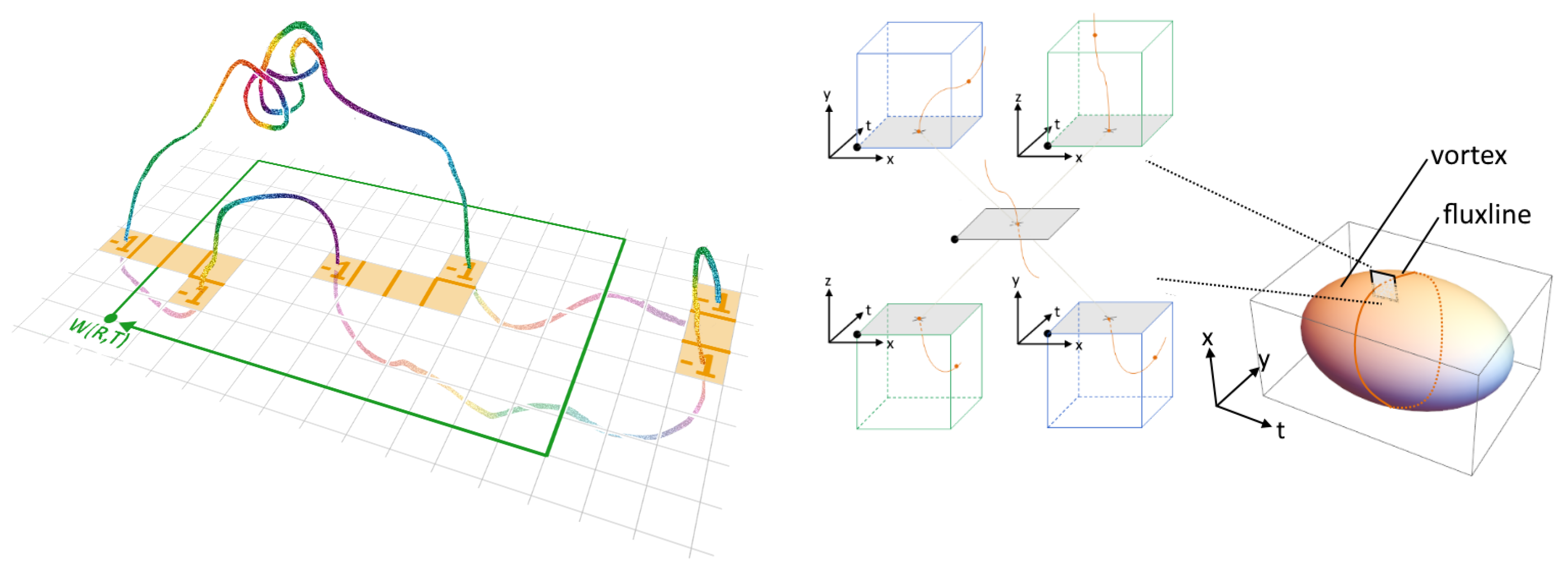
The center vortex model of Quantum Chromodynamics [1,2] explains confinement [3] and chiral symmetry breaking [4,5,6] by the assumption that the relevant excitations of the QCD vacuum are Center vortices, closed color magnetic flux lines evolving in time. In four-dimensional space-time, these closed flux lines form closed surfaces in dual space, see Figure 1. In the low-temperature phase, they percolate space-time in all dimensions.
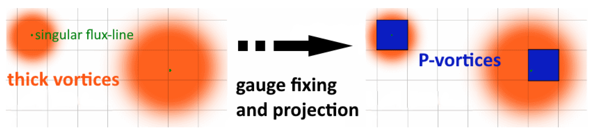
In Maximal Center gauge, the center vortex surface can be detected by the identification of Wilson loops evaluating to non-trivial center elements and by projecting the links to the center degrees of freedom—the piercing of a Wilson loop by a center flux line contributes a non-trivial factor to the numerical value of the loop. The detection of plaquettes pierced by a flux line is schematically shown in Figure 2.
The vortex flux has a finite thickness, but is located by thin P-vortices. As long as these P-vortices successfully locate vortices, we speak of a valid vortex-finding property. A problem concerning this property was discovered by Bornyakov et al. [7]. We were able to resolve these problems using an improved version of the gauge-fixing routines [8,9,10] and could show, for relatively small lattices, that center vortices reproduce the string tension. We found hints towards a color structure existing on the vortex surface [11]. This color structure might be directly related to the topological charge of center vortices and could lead to a more detailed explanation of their chiral properties. Their study is especially complicated by the fact that measurements of the topological charge require sufficiently smooth field configurations, whereas the quality of the center vortex detection suffers with increasing smoothness of the lattice, that is, the vortex-finding property can get lost during smoothing or cooling of the lattice. We want to bring more light to these difficulties by an analysis of the following:
- Correlation between color structure and surface curvature,
- Size of color-homogeneous regions on the surface, and
- Influence of cooling on color-homogeneous regions on the surface, and
- Influence of smoothing the vortex surface on color-homogeneous regions.
As this is the first time these measurements are performed with our algorithms, this work is to be understood as a proof of concept.
2. Materials and Methods
Our lattice simulation is based on gluonic SU(2) Wilson action with inverse coupling covering an interval from to in steps of . The corresponding lattice spacing a is determined by a cubic interpolation of literature values given in Table 1 and complemented by an extrapolation according to the asymptotic renormalization group equation
We assume a physical string tension of . Our analysis is performed on lattices of size , and and .
We use an improved version of maximal center gauge to identify the position of the flux lines building up the vortex surface via center projection. The improvements are described in detail in the Refs. [8,9,10] and identify non-trivial center regions by perimeters evaluating to non-trivial center elements. These regions are used as guidance for maximal center gauge. By simulated annealing, we look for gauge matrices SU(2) at each lattice point x, so that the functional
is maximized. After fixing the gauge, we project to center degrees of freedom and identify the non-trivial plaquettes, but save the un-projected lattice for our measurements concerning the color structure.
These measurements are based on the S2-homogeneity which compares the color vector of two plaquettes related to the same lattice point. With the two plaquettes written as , the S2-homogeneity is defined as

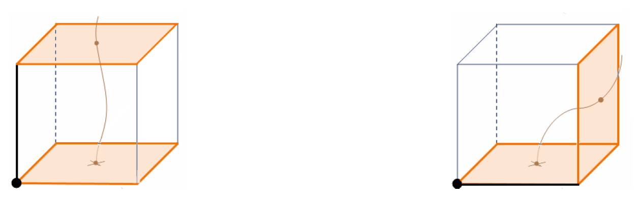
By calculating the S2-homogeneity of two plaquettes that are pierced by a center flux-line, we restrict the measurement to the vortex surface, and can distinguish the two scenarios depicted in Figure 3:
- Parallel plaquettes corresponding to a weakly curved flux-line, that is, plaquettes located in the same plane in dual space.
- Orthogonal plaquettes, plaquettes that are neighbours in dual space but have different orientation, corresponding to strongly curved flux-lines,
As the curvature of the flux-line directly correlates to the curvature of the vortex surface, this allows an analysis of the correlation between S2-homogeneity and curvature of the vortex surface.
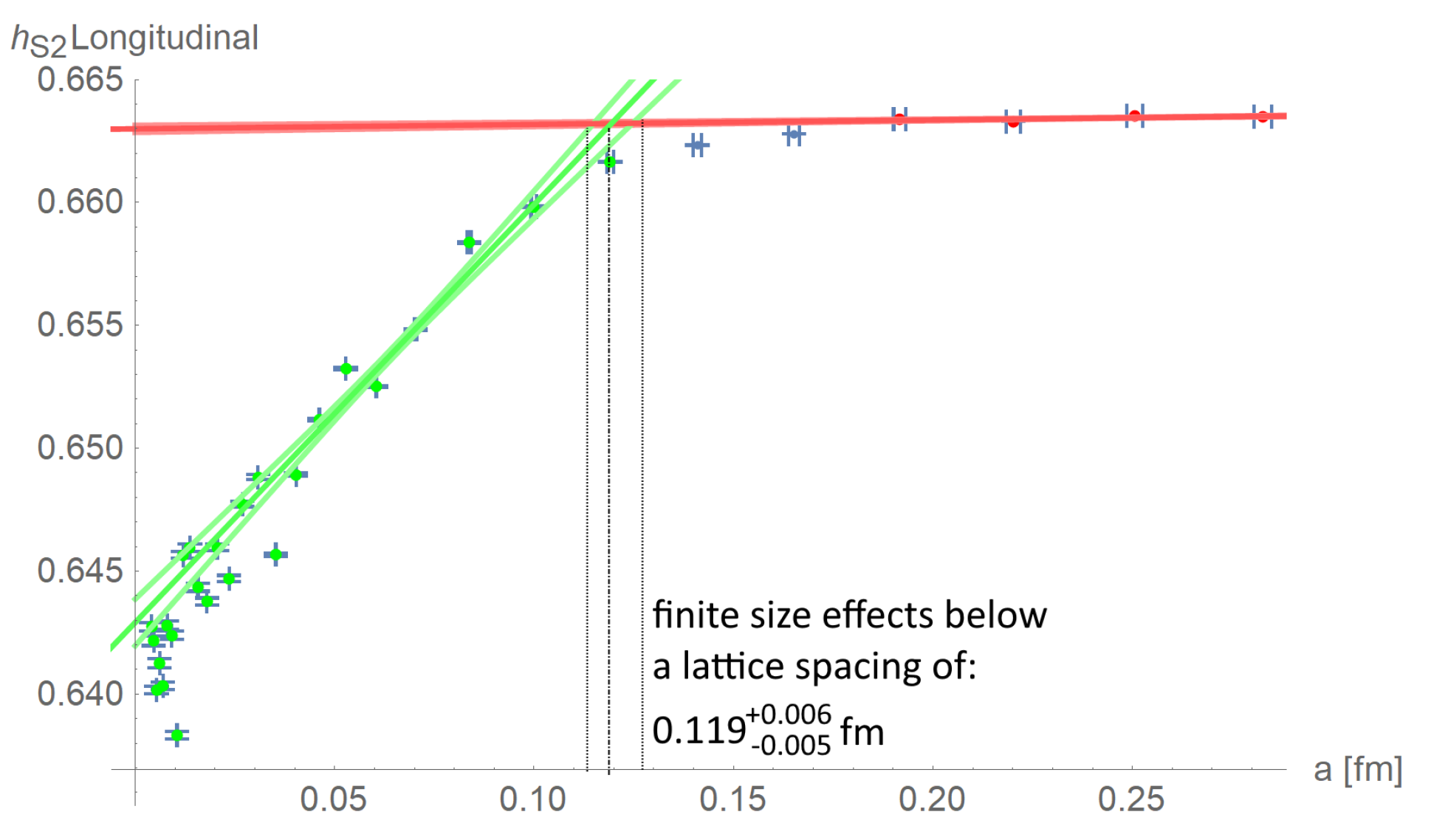
Calculating the S2-homogeneity for different lattice spacings and lattice sizes allows to examine the size of homogeneous regions on the vortex surface by exploiting finite-size effects. We assume that for sufficiently big lattices, the S2-homogeneity is independent of the lattice size and, at most, linear-dependent on the lattice spacing. As long as the color structure fits into the lattice, we assume a decoupling of this structure from the lattice parameters. Shrinking the lattice by reducing the lattice spacing allows to identify the physical lattice extent below which finite size effects introduce stronger dependencies on the lattice parameters, see Figure 4.
Varying the physical lattice size by changing the number of lattice sites and repeating the procedure, we can check whether these finite size effects define a physical scale independent of the lattice parameters—at the onset of the finite size effects, the lattice spacing times the lattice size should be a constant defining the size of color-homogeneous regions on the vortex surface. With decreasing lattice sizes, the onset of the finite size effects occurs at lower values of ; hence, we choose small lattices to perform these measurements. As this procedure requires sufficiently good statistics at high values of , we include in the averages all pairs of plaquettes belonging to the same P-vortex.
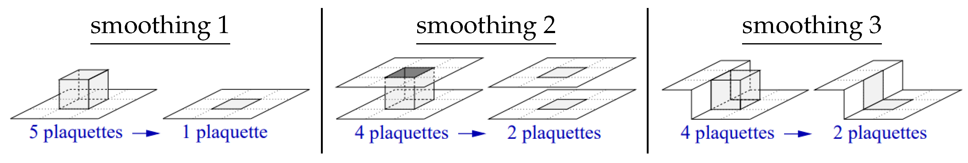
For measurements of topological properties, sufficiently smooth configurations are required, but smooth configurations complicate the vortex detection. There are many different procedures for generating such smooth configurations or smoothing excitations belonging to specific degrees of freedom. We use Pisa Cooling [17] with a cooling parameter of 0.05. Repeating the aforementioned measurements in cooled configurations, we compare the influence of a direct smoothing of the vortex surface, described in detail in [18,19], with the effects of cooling. The smoothing procedure consists of “cutting out” parts of the vortex surface and “sewing together” the surface again, see Figure 5.
Additional to the three depicted procedures, we have “smoothing 0”, which deletes isolated unit-cubes and is part of all other listed smoothing routines. All smoothing procedures remove short-range fluctuations from the vortex surface and are considered to have no influence on the infra-red degrees of freedom, but smoothing two has an influence on the connectivity of the vortex surface in contrast to the other smoothing methods.
3. Results
We start by presenting our findings concerning the correlation between the color structure and surface curvature of vortices. The measurements were performed on lattices of size , and the data show a clear distinction between weakly and strongly curved parts of the vortex surface with respect to S2-homogeneity: the more the vortex surface is curved, the smaller the value of the color-homogeneity.
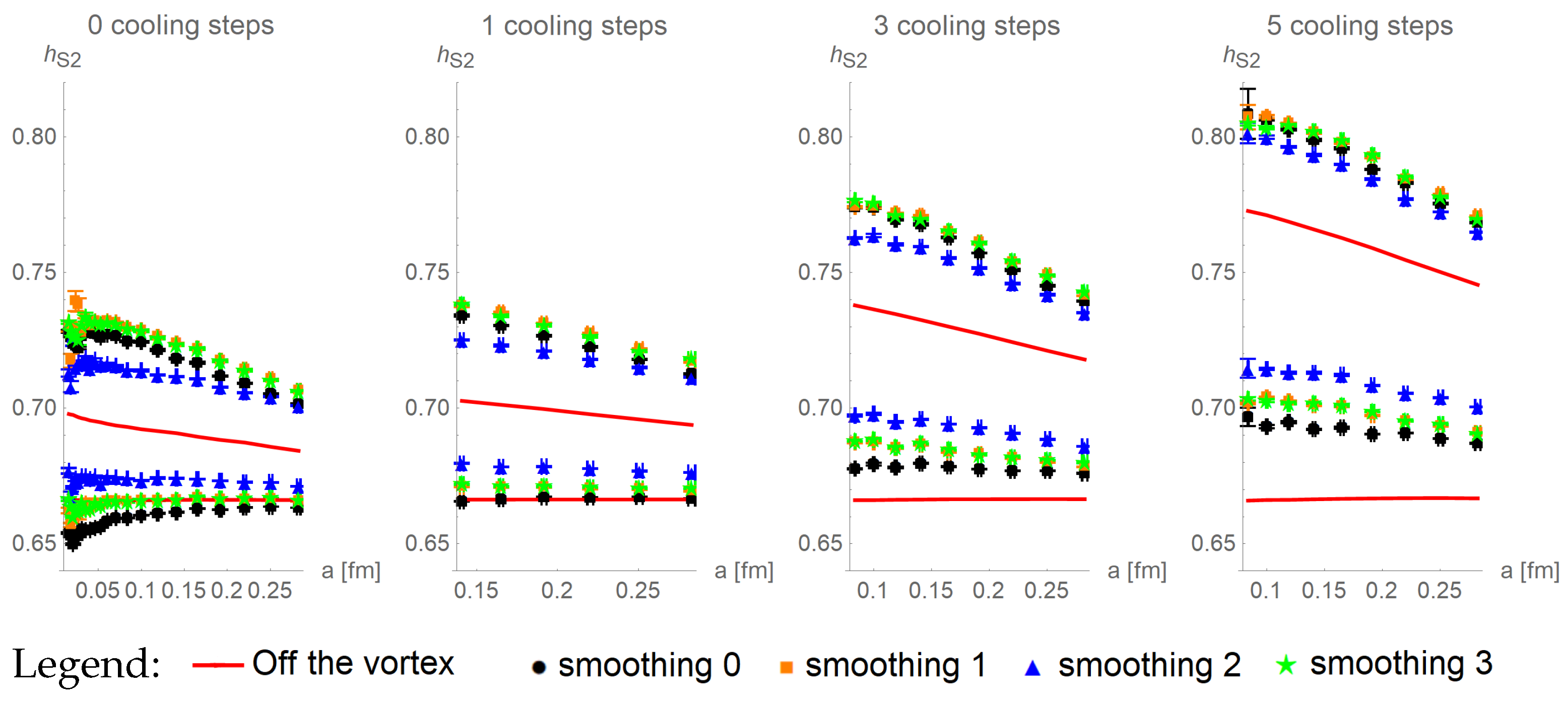
This can be seen in Figure 6, where we show distinct evaluations of the S2-homogeneity for parallel plaquette pairs (larger values) and orthogonal plaquette pairs (smaller values) for various smoothing and cooling steps. The difference between parallel and perpendicular plaquettes indicates a clear correlation of fluctuations in color space to fluctuations in space-time. increases with more intense cooling, especially for parallel plaquettes. Additionally, the mentioned difference and the correlation increases. It is interesting to observe that with cooling, this difference between parallel and perpendicular plaquette pairs increases more for pairs off the vortex (red lines) than for pairs on P-vortices (data points). For 0 cooling steps, the difference between the red lines is roughly 50% of the difference between data points. This difference increases to ≈ for five cooling steps. Since the thickness of vortices increases with cooling and P-vortices stay thin, “off the P-vortex” can still be “on the thick vortex” and those pairs “on the thick vortex” contribute to the “off the vortex” averages. This shows that the correlation between curvature and S2-homogeneity is a property of the thick vortices, and not of the surrounding vacuum.
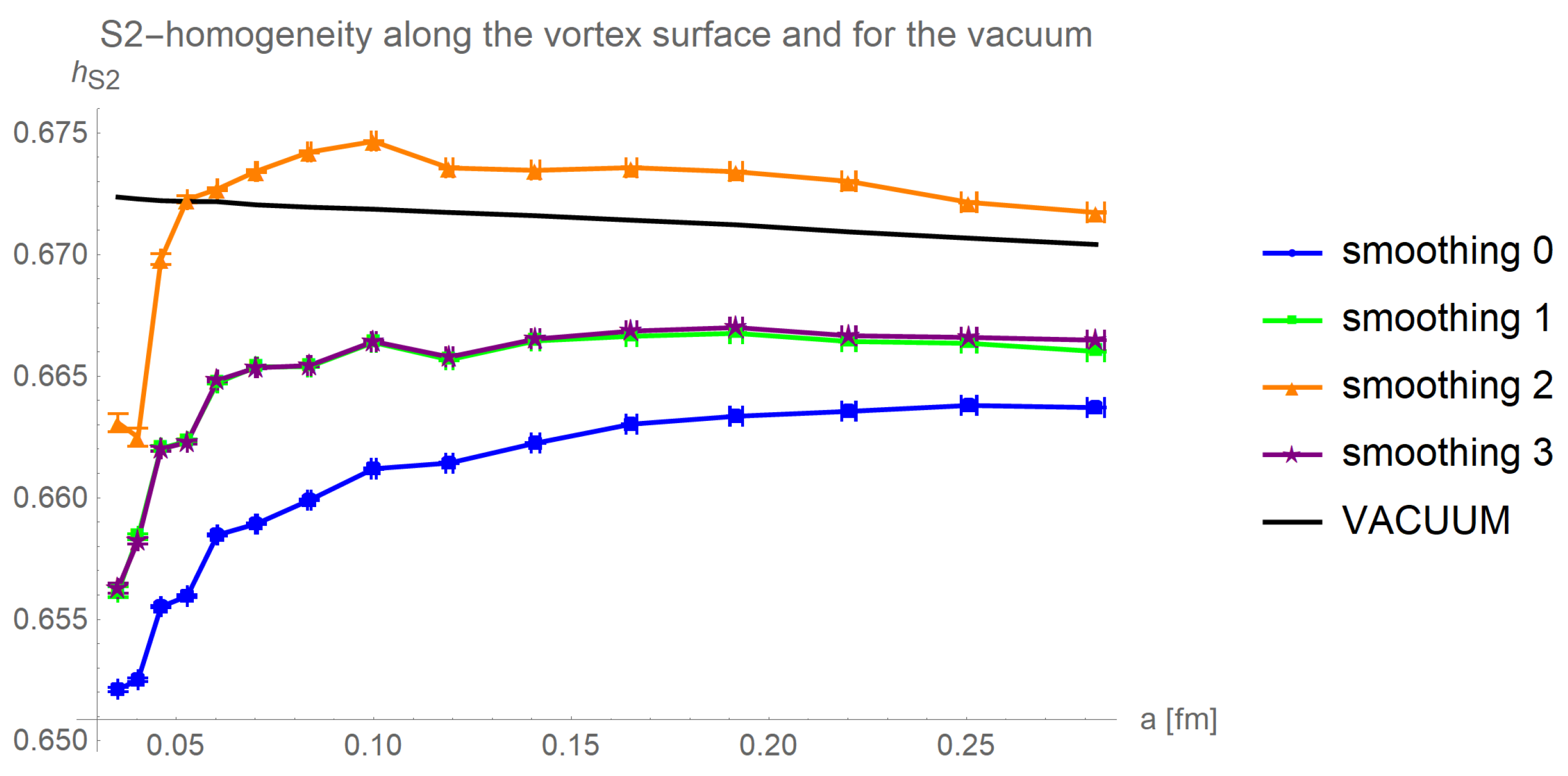
Comparing the different smoothing procedures, it can be seen that smoothing 1 and smoothing 3 lead to quantitatively identical results, with a homogeneity raised above those of smoothing 0. With smoothing 2, the difference between weak and strong curvature is reduced: The homogeneity of weak curvature is decreased, and the homogeneity of strong curvature increased. As smoothing 2 is the only procedure influencing the connectivity of the vortex surface, we conclude that this connectivity might be of importance in further considerations of the color structure, and that smoothing 2 should be used with care. This is strengthened by the fact that smoothing 2 results in the vortex becoming overall more homogeneous than the vacuum, see Figure 7.
A non-trivial color structure is indicated by color inhomogeneities, hence we suspect that smoothing 2 cuts out parts of the vortex surface that might carry potential color structure.
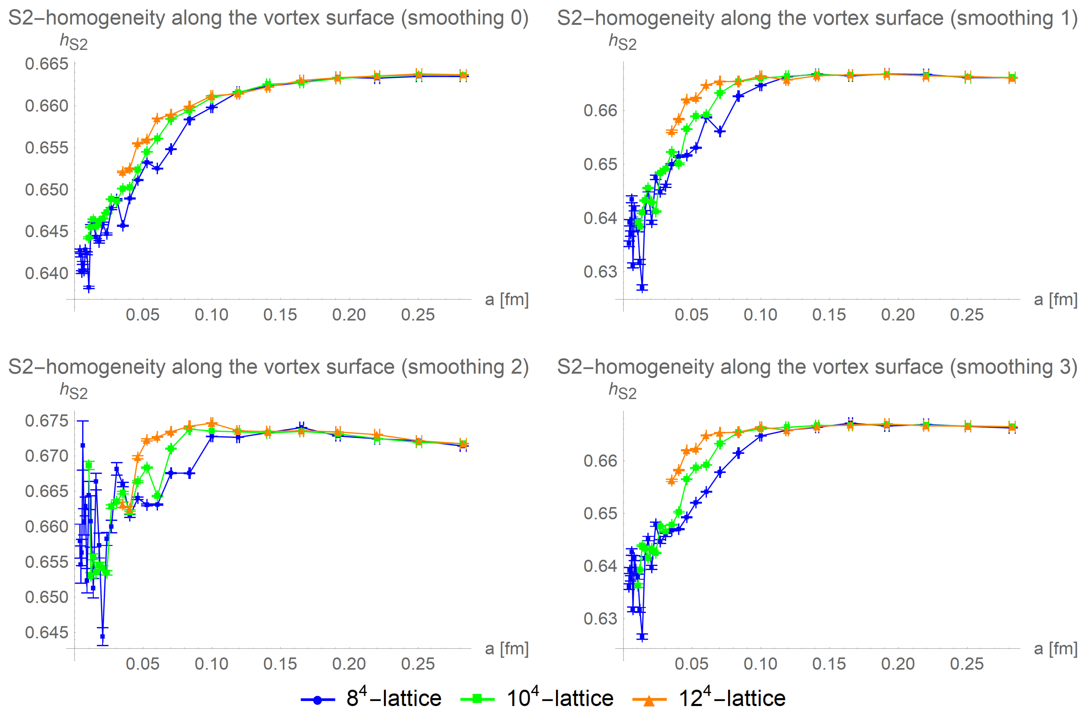
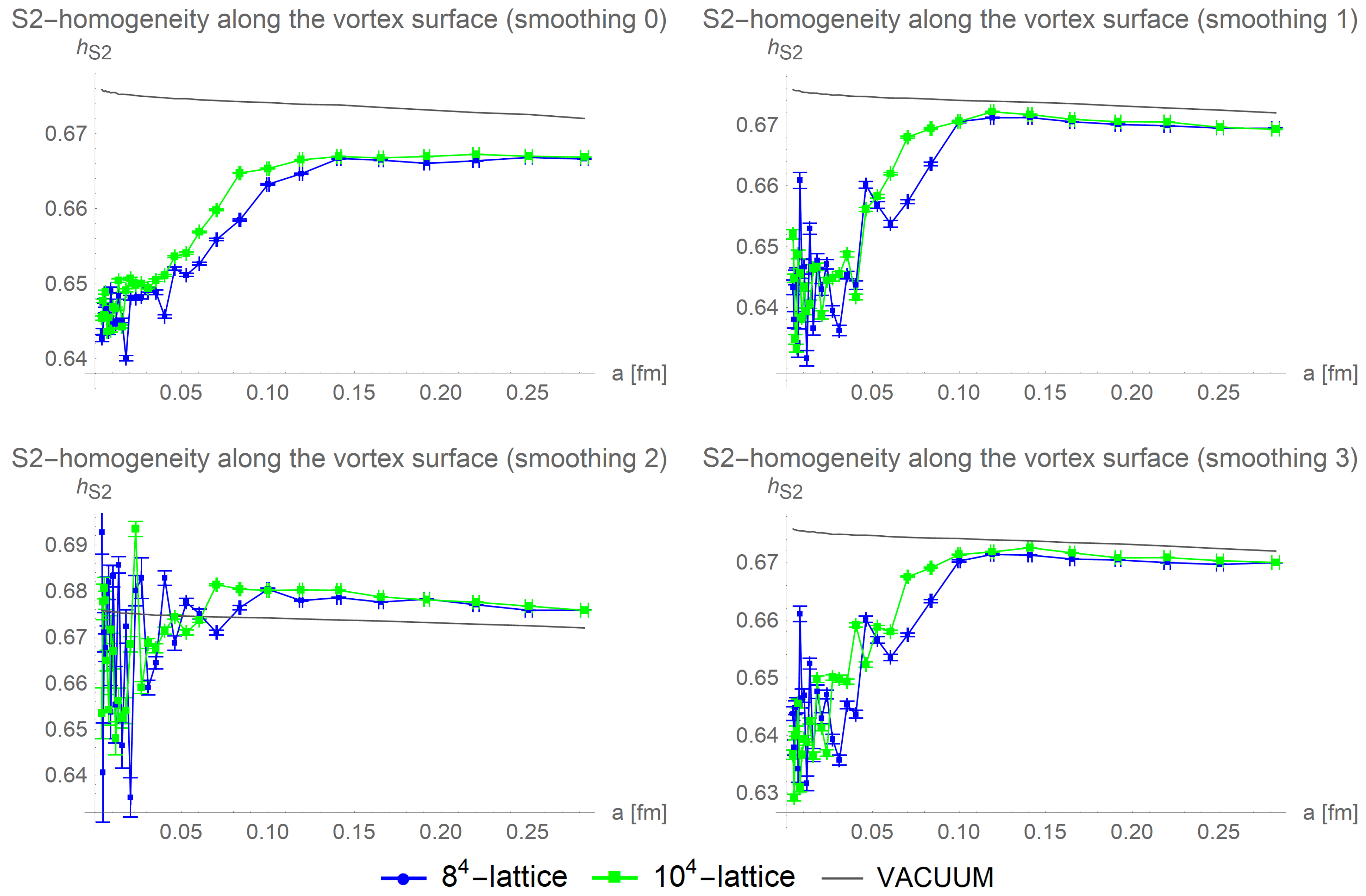
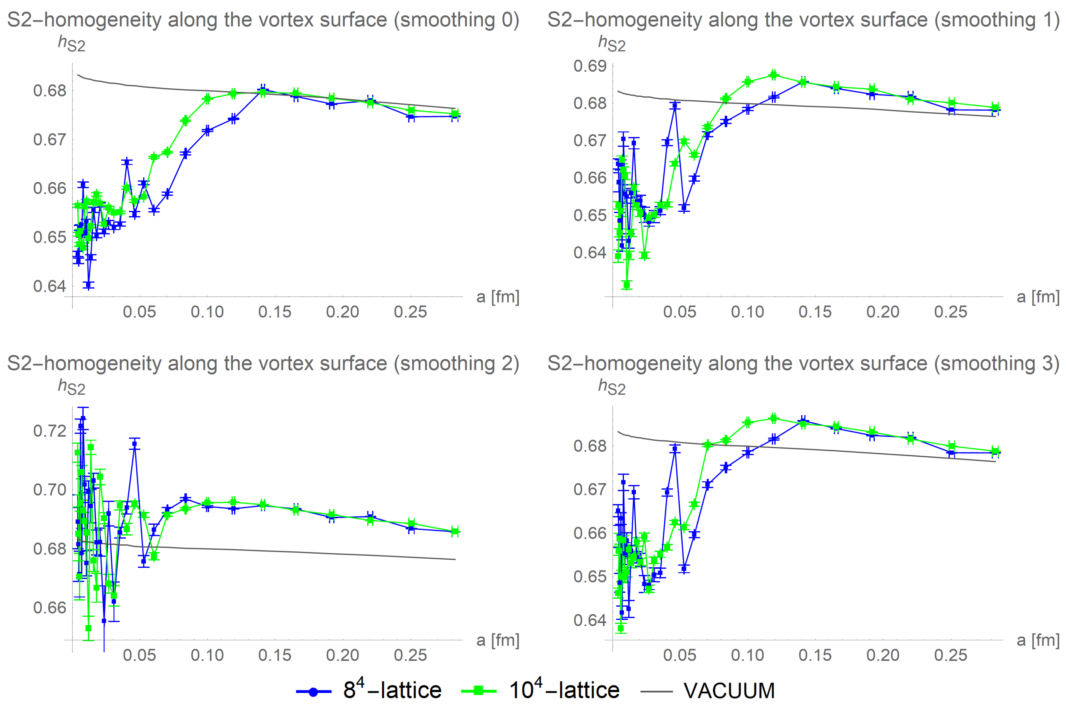
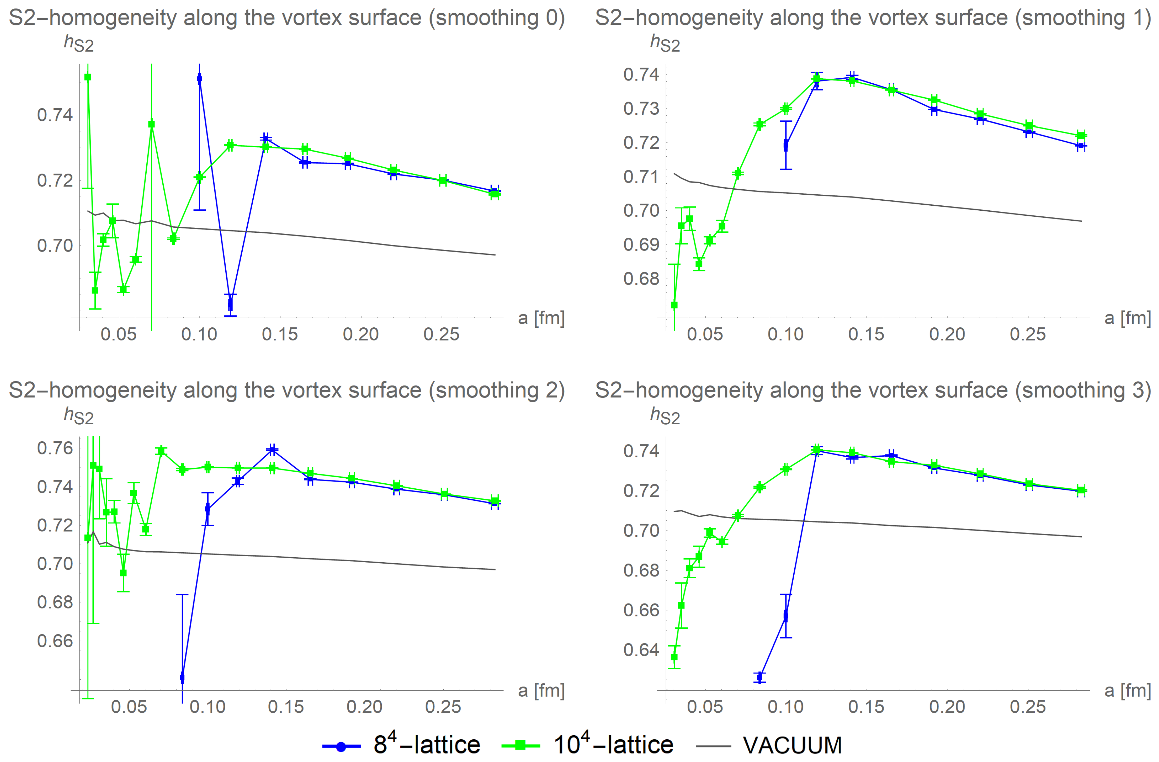
The dependency of the S2-homogeneity on the physical lattice volume allows a more detailed investigation of the color structure on the vortex surface. In Figure 8, we compare the S2-homogeneity along the vortex surface for different lattice sizes and smoothing procedures. We find a loss of the S2-homogeneity for small lattice volumes and give arguments that the loss of the homogeneity is caused by finite size effects, indicating a physical non-vanishing size of color-homogeneous regions. We estimate the size of these homogeneous regions by linear fits to the values of the S2-homogeneity in the large and small volume regions, as shown in Figure 4. This procedure is applied to different lattice sizes and numbers of cooling steps.
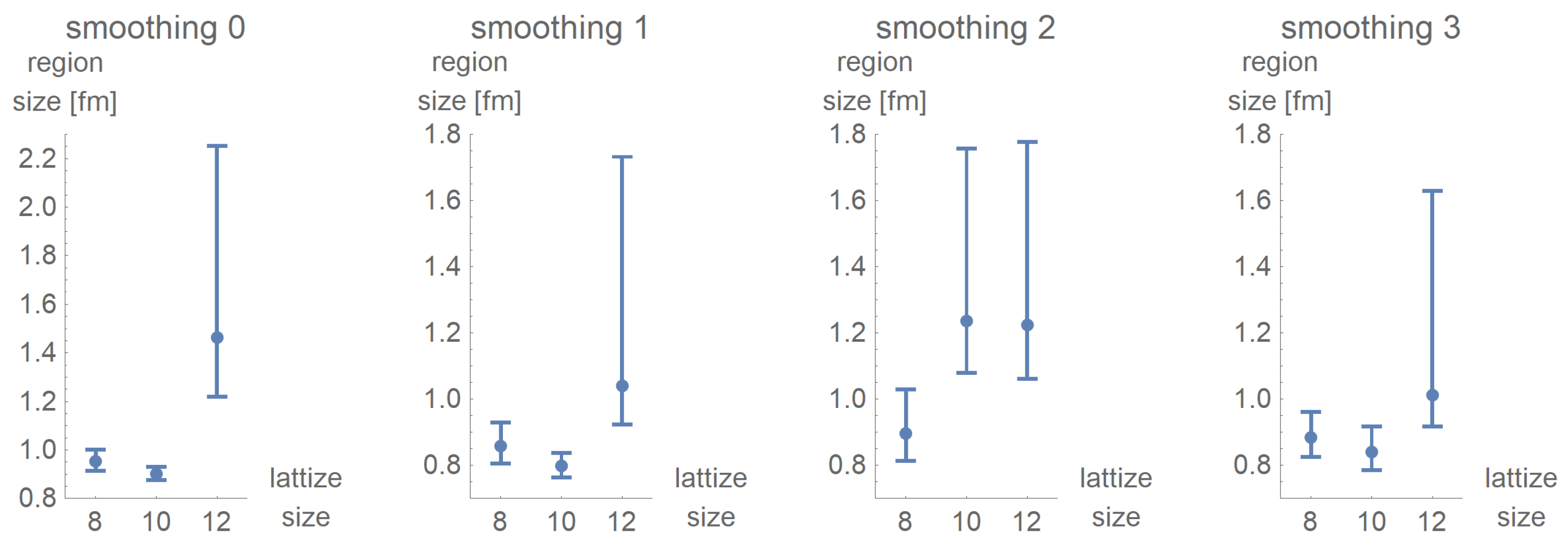
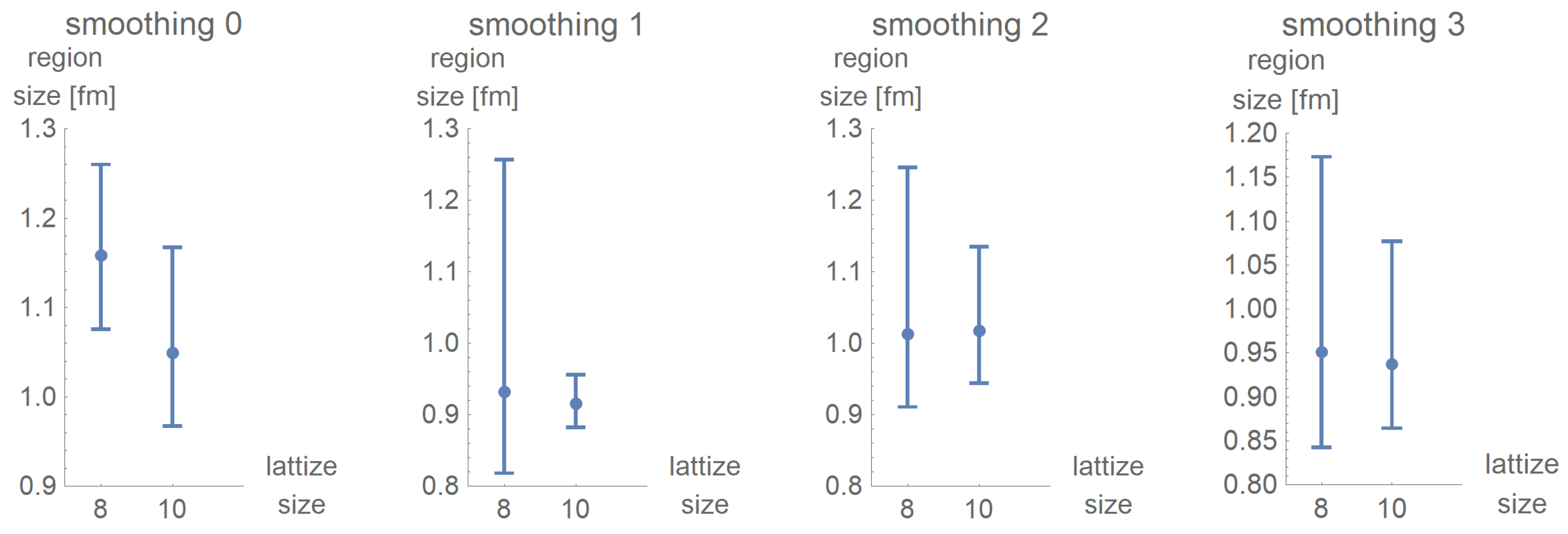
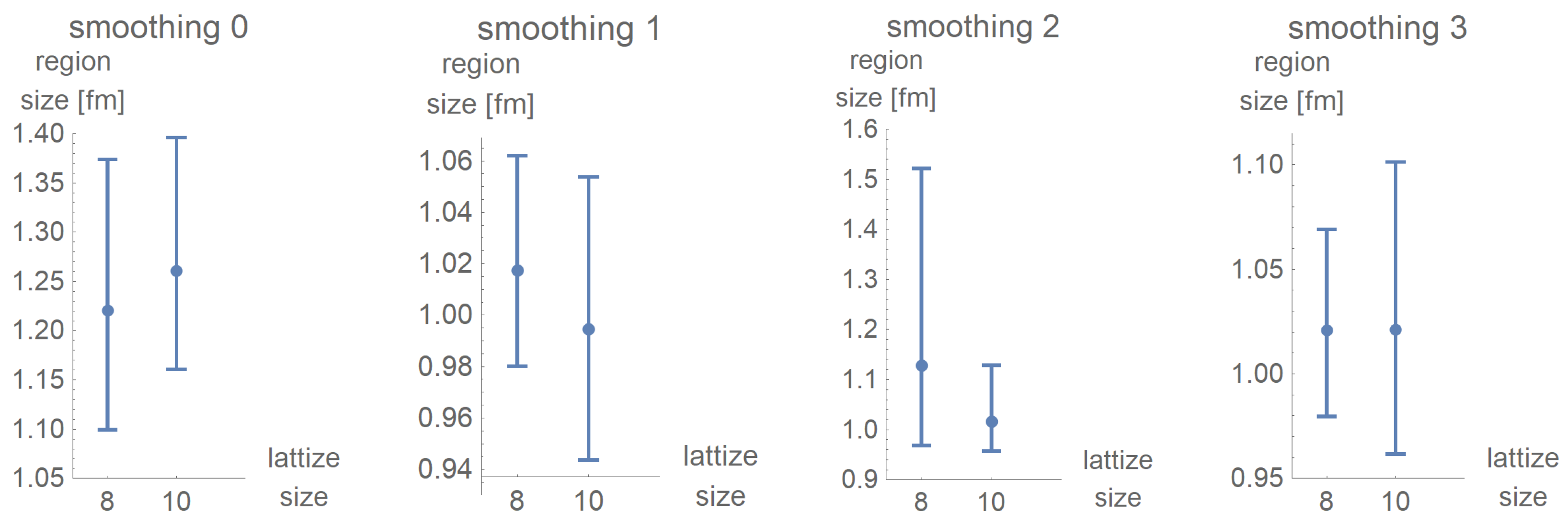
Multiplying the lattice spacing at the intersection with the lattice extent, we estimate the size of the homogeneous regions. In Figure 9, it can be seen that the values are compatible within errors for smoothing 0, smoothing 1, and smoothing 3 on lattices of size and . The measurements in lattices of size result in higher values with bigger errors.
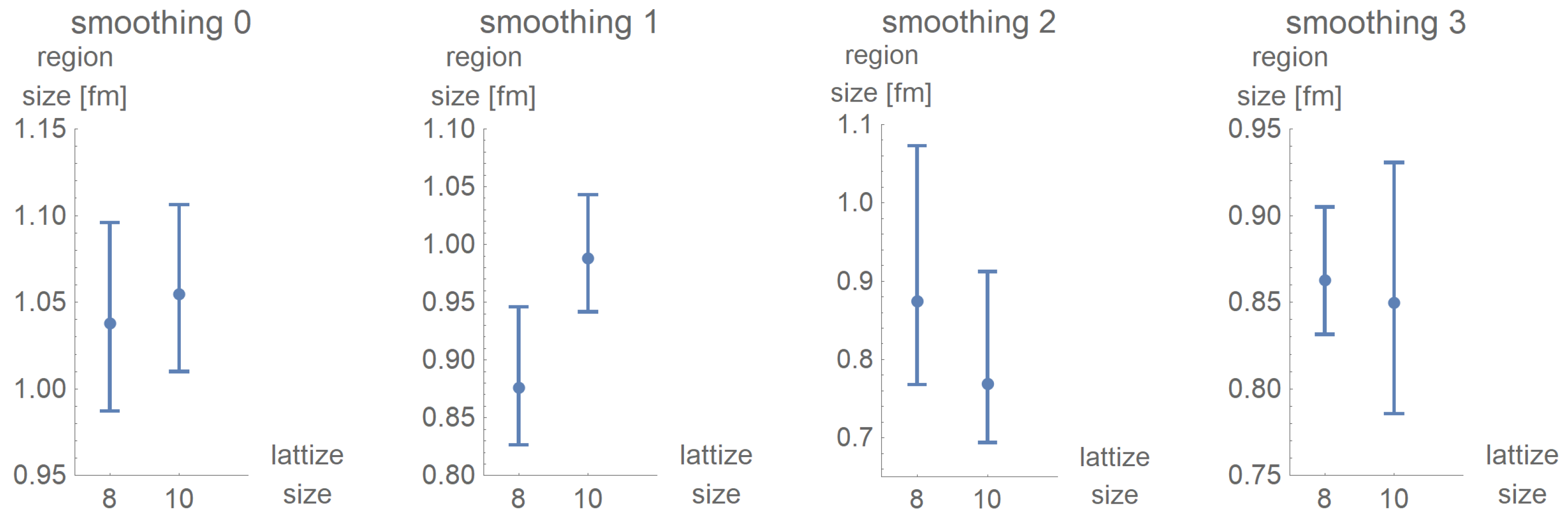
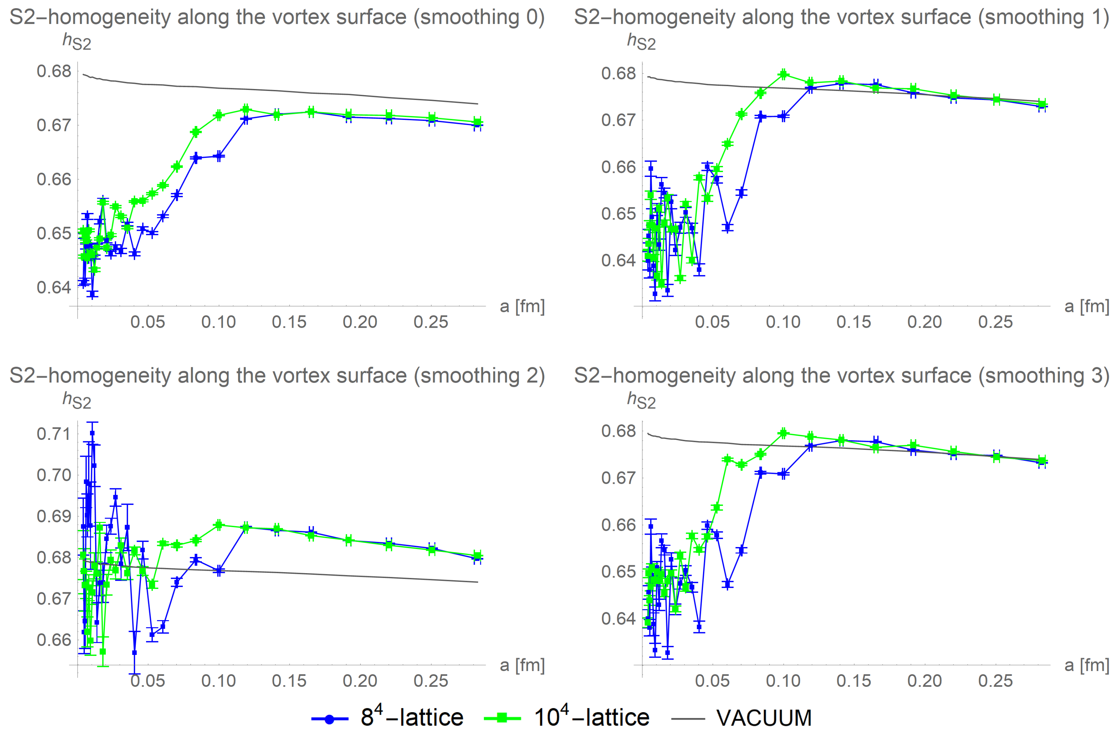
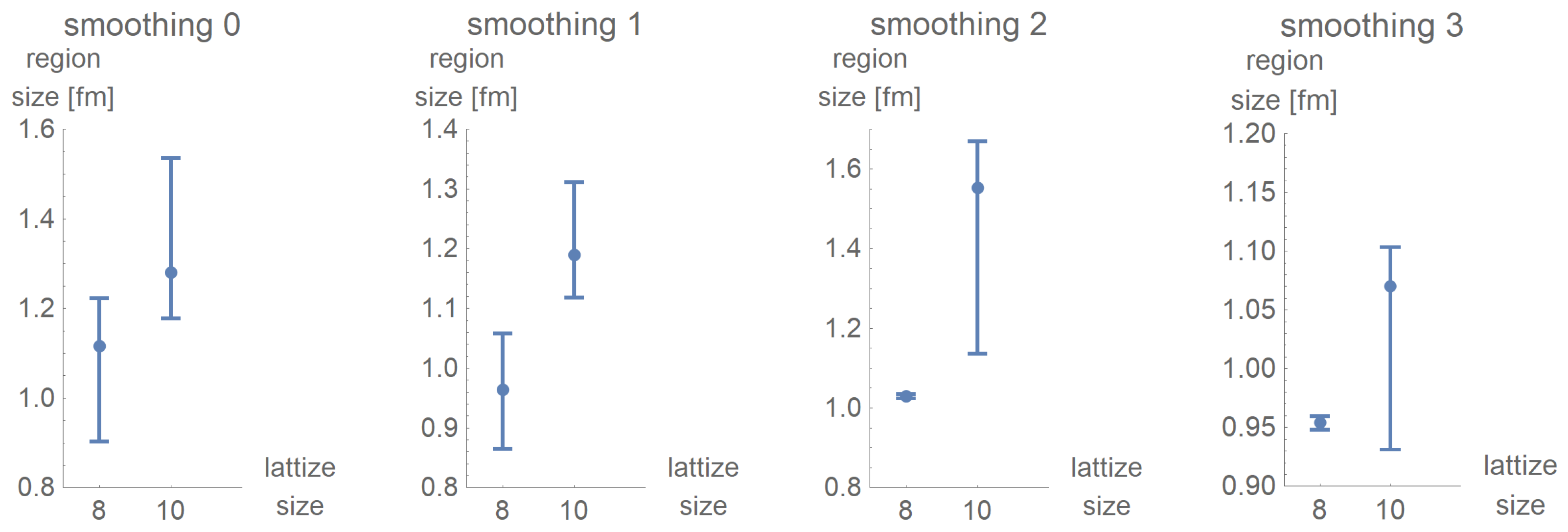
The estimate of the size of the homogeneous regions is repeated for different numbers of cooling steps in lattices of size and . This allows to infer the influence of the smoothness of the lattice on homogeneous regions. In Figure 10, the S2-homogeneities are shown after one cooling step.
Of interest is that with cooling the S2-homogeneities of the different smoothing procedures become more and more similar to those of smoothing 2. In Figure 11 the corresponding sizes of the color homogeneous regions are shown.
After two cooling steps, smoothing 1 results in the S2-homogeneity of the vortex becoming no longer distinguishable from the vacuum, see Figure 12.
A small increase in the size of homogeneous regions is observable, see Figure 13.
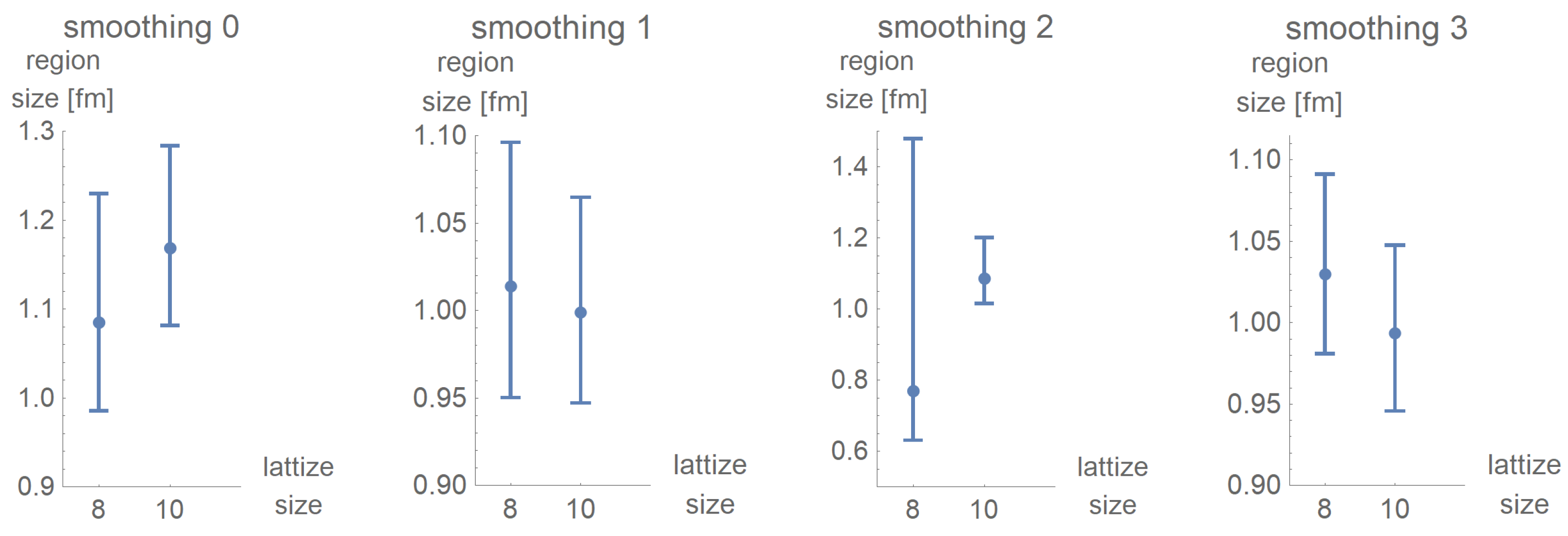
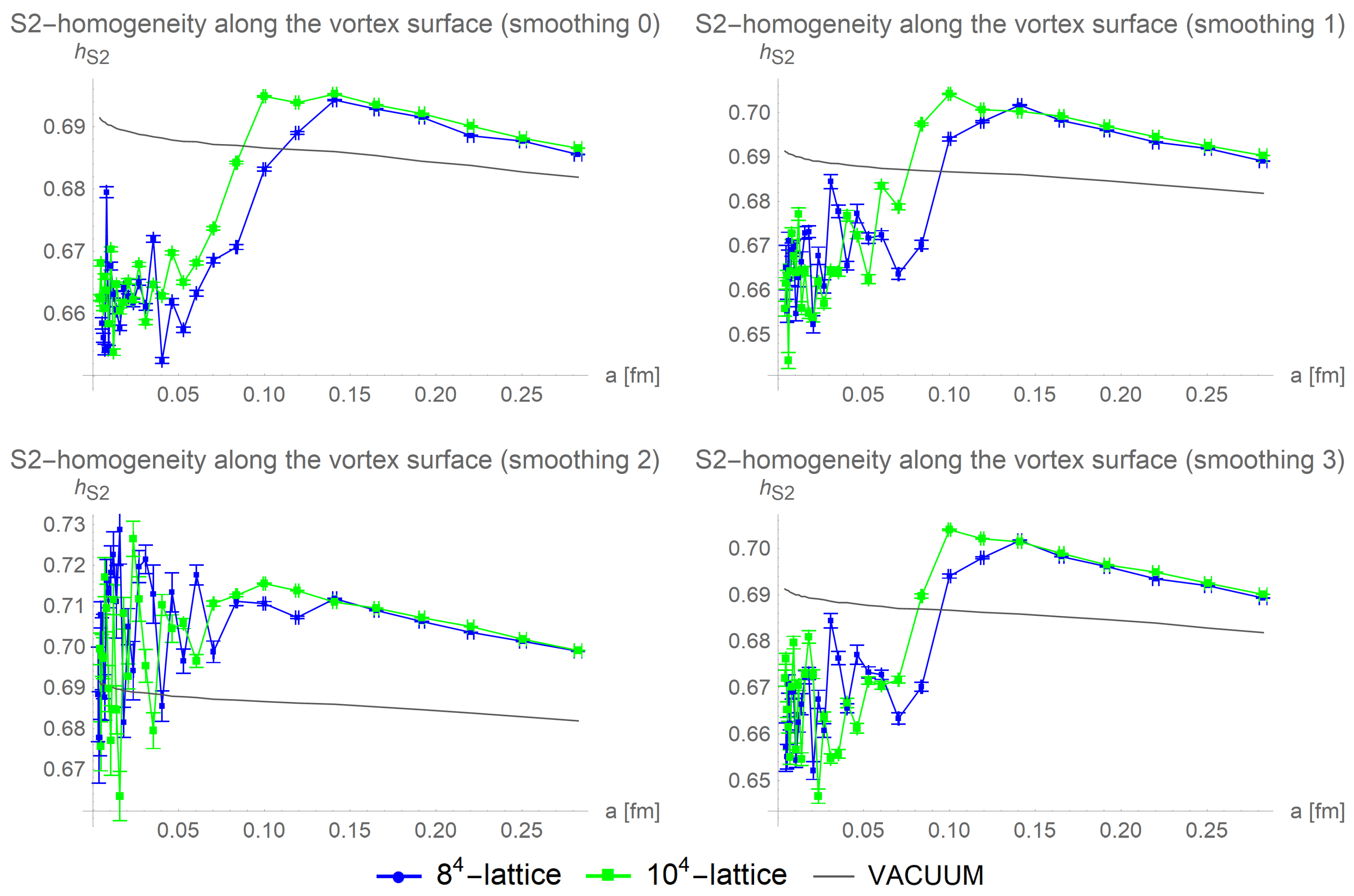
After three cooling steps, smoothing 1, smoothing 2, and smoothing 3 result in the S2-homogeneity of the vortex growing above those of the vacuum, while the homogeneity of smoothing 0 is no longer distinguishable from those of the vacuum, see Figure 14. The corresponding size of the color homogeneous regions is shown in Figure 15.
After five cooling steps, all smoothing procedures result in the vortex becoming more homogeneous than the vacuum as is depicted in Figure 16. The corresponding size of the color homogeneous regions is shown in Figure 17.
The calculations with 10 cooling steps were complicated by a loss of the vortex-finding property. In many of the configurations with 10 cooling steps, no vortices could be detected, making the configurations unusable for analyzing color structures on the vortex surface. The cause for this loss of the vortex-finding property and a possible resolution is of special interest, as it hints at possible ways to improve the vortex detection algorithms. This topic is discussed in another article [20]. The S2-homogeneities of the usable part of the data are shown in Figure 18.
The line fits used to identify the onset of the finite size effects became problematic, causing a possible underestimation of the error; hence, data resulting from 10 cooling steps should be taken with care. The corresponding size of the color homogeneous regions is shown in Figure 19.
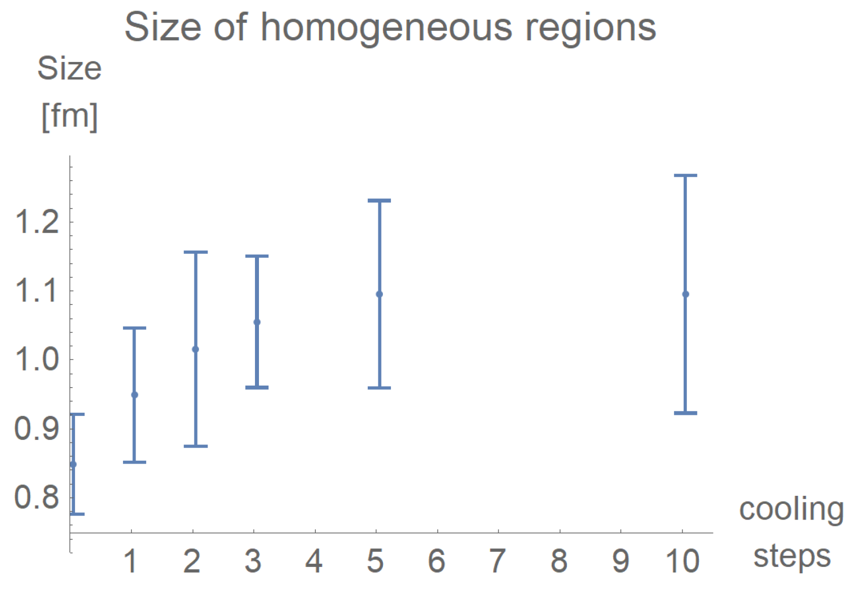
As the error bars result from intersections of line fits, they are not necessarily symmetric. To combine the data, the error bar was interpreted as two separate datapoints. Using the data from the lattize sizes and with smoothing 0, smoothing 1, and smoothing 3, we estimate the size of the homogeneous regions to the values shown in Figure 20.
The estimation starts at fm without cooling, reaching fm after 10 cooling steps. This increase seems to have a maximal value, that is, cooling does not let the size of homogeneous regions increase to infinity. The dependency of the S2-homogeneities on the lattice spacing below the onset of the finite size effects showed hints at a stepwise reduction. Distinguishing whether these resulted from random fluctuations of our data or were caused by a quantization of the sizes of the homogeneous regions might be possible with more lattice data.
4. Discussion
Our results show that curvature of flux lines correlates with fluctuations in color space. This correlation becomes stronger when cooling procedures are applied, but weakens when the connectivity of the vortex surface is harmed. The correlation seems to be a special feature along the center vortex surface, as it weakens when restricting the analysis to plaquettes that are not pierced.
As intersections and twistings of vortices can produce topological charge and the twisting of the vortex is correlated to color fluctuations, see [21], our data strengthens the assumption that the color structure of vortices directly relates to topological charge, enabling center vortices to explain chiral symmetry breaking.
Complications concerning measurements of the topological charge and center vortices raise the question of whether the topological properties of center vortices get lost during cooling, or if the properties are kept but the vortex detection fails. Our data indicate the latter because a possible loss of the color structure due to expanding color homogeneous regions on the vortex surface is not probable, as the size of these regions seems to be bound by an upper limit. Cooling increases the S2-homogeneity of the Vortex more than it increases the homogeneity of the vacuum.
The finite size of these color homogeneous regions is of further interest, concerning the question whether the vortex surface covers the defining the color space or not. It indicates that finite areas on this color cannot correspond to arbitrarily big areas on the vortex surface.
To stay sufficiently far away from finite size effects and guarantee a sufficiently high resolution concerning homogeneous regions, our advice is to keep the physical lattice volume well above, and the lattice spacing well below 0.78 fm. As our analysis at a higher number of cooling steps suffered from a loss of the vortex-finding property, further improvements at detecting center vortices in lattice simulations are needed. Further analysis of this loss of the vortex finding property is to be published in [20].
Author Contributions
Conceptualization, R.G. and M.F.; Formal analysis, R.G.; Investigation, R.G.; Software, R.G. and M.F.; Supervision, M.F.; Writing—original draft, Rudolf Golubich; Writing—review & editing, M.F. All authors have read and agreed to the published version of the manuscript.
Funding
This research received no external funding.
Institutional Review Board Statement
Not applicable.
Informed Consent Statement
Not applicable.
Data Availability Statement
The data presented in this study are available on request from the corresponding author.
Acknowledgments
We thank the company Huemer-Group (www.huemer-group.com, accessed on 3 March 2021) and Dominik Theuerkauf for providing the computational resources speeding up our calculations.
Conflicts of Interest
The authors declare no conflict of interest.
References
- ’t Hooft, G. On the phase transition towards permanent quark confinement. Nucl. Phys. B 1978, 138, 1–25. [Google Scholar] [CrossRef]
- Cornwall, J.M. Quark confinement and vortices in massive gauge-invariant QCD. Nucl. Phys. B 1979, 157, 392–412. [Google Scholar] [CrossRef]
- Del Debbio, L.; Faber, M.; Giedt, J.; Greensite, J.; Olejnik, S. Detection of center vortices in the lattice Yang-Mills vacuum. Phys. Rev. D 1998, 58, 094501. [Google Scholar] [CrossRef] [Green Version]
- Faber, M.; Höllwieser, R. Chiral symmetry breaking on the lattice. Prog. Part. Nucl. Phys. 2017, 97, 312–355. [Google Scholar] [CrossRef] [Green Version]
- Höllwieser, R.; Schweigler, T.; Faber, M.; Heller, U.M. Center Vortices and Chiral Symmetry Breaking in SU(2) Lattice Gauge Theory. Phys. Rev. 2013, D88, 114505. [Google Scholar] [CrossRef] [Green Version]
- Höllwieser, R. Center Vortices and Topological Charge. arXiv 2017, arXiv:hep-lat/1706.06436. [Google Scholar]
- Bornyakov, V.G.; Komarov, D.A.; Polikarpov, M.I.; Veselov, A.I. P vortices, nexuses and effects of Gribov copies in the center gauges. In Proceedings of the Quantum Chromodynamics and Color Confinement, Proceedings, International Symposium, Confinement 2000, Osaka, Japan, 7–10 March 2000; eprint: hep-lat/0210047 reportNumber: ITEP-LAT-2002-18. pp. 133–140. [Google Scholar]
- Golubich, R.; Faber, M. The Road to Solving the Gribov Problem of the Center Vortex Model in Quantum Chromodynamics. Acta Phys. Pol. B Proc. Suppl. 2020, 13, 59–65. [Google Scholar] [CrossRef]
- Golubich, R.; Faber, M. Center Regions as a Solution to the Gribov Problem of the Center Vortex Model. Acta Phys. Pol. B Proc. Suppl. 2021, 14, 87. [Google Scholar] [CrossRef]
- Golubich, R.; Faber, M. Improving Center Vortex Detection by Usage of Center Regions as Guidance for the Direct Maximal Center Gauge. Particles 2019, 2, 30. [Google Scholar] [CrossRef] [Green Version]
- Golubich, R.; Faber, M. Thickness and Color Structure of Center Vortices in Gluonic SU(2) QCD. Particles 2020, 3, 31. [Google Scholar] [CrossRef]
- Bali, G.S.; Schlichter, C.; Schilling, K. Observing long color flux tubes in SU(2) lattice gauge theory. Phys. Rev. D 1995, 51, 5165–5198. [Google Scholar] [CrossRef] [PubMed] [Green Version]
- Booth, S.P.; Hulsebos, A.; Irving, A.C.; McKerrell, A.; Michael, C.; Spencer, P.S.; Stephenson, P.W. SU(2) potentials from large lattices. Nucl. Phys. 1993, B394, 509–526. [Google Scholar] [CrossRef] [Green Version]
- Michael, C.; Teper, M. Towards the Continuum Limit of SU(2) Lattice Gauge Theory. Phys. Lett. 1987, B199, 95–100. [Google Scholar] [CrossRef]
- Perantonis, S.; Huntley, A.; Michael, C. Static Potentials From Pure SU(2) Lattice Gauge Theory. Nucl. Phys. 1989, B326, 544–556. [Google Scholar] [CrossRef]
- Bali, G.S.; Fingberg, J.; Heller, U.M.; Karsch, F.; Schilling, K. The Spatial string tension in the deconfined phase of the (3+1)-dimensional SU(2) gauge theory. Phys. Rev. Lett. 1993, 71, 3059–3062. [Google Scholar] [CrossRef] [PubMed] [Green Version]
- Campostrini, M.; Di Giacomo, A.; Maggiore, M.; Panagopoulos, H.; Vicari, E. Cooling and the String Tension in Lattice Gauge Theories. Phys. Lett. B 1989, 225, 403–406. [Google Scholar] [CrossRef]
- Bertle, R. The Vortex Model in Lattice Quantum Chromo Dynamics. Dissertation. 2005. Available online: http://www.ub.tuwien.ac.at/diss/AC04798186.pdf (accessed on 3 March 2021).
- Bertle, R.; Engelhardt, M.; Faber, M. Topological susceptibility of Yang-Mills center projection vortices. Phys. Rev. D 2001, 64. [Google Scholar] [CrossRef] [Green Version]
- Golubich, R.; Faber, M. A possible resolution to troubles of SU(2) center vortex detection in smooth lattice configurations. Universe. submitted.
- Höllwieser, R.; Faber, M.; Heller, U.M. Intersections of thick center vortices, Dirac eigenmodes and fractional topological charge in SU(2) lattice gauge theory. J. High Energy Phys. 2011, 2011. [Google Scholar] [CrossRef] [Green Version]
Figure 1.
(left) After transformation to maximal center gauge and projection to the center degrees of freedom, a flux line can be traced by the following non-trivial plaquettes. (right) Due to the evolution in time, such a flux can be traced in two dimensions. In dual space, it results in a closed surface.

Figure 2.
Vortex detection as a best-fit procedure of P-Vortices to thick vortices shown in a two-dimensional slice through a four-dimensional lattice.
Figure 2.
Vortex detection as a best-fit procedure of P-Vortices to thick vortices shown in a two-dimensional slice through a four-dimensional lattice.

Figure 3.
Depicted are two plaquettes that are related to the same lattice-point via parallel transport along the single edge depicted as a thicker black line. We distinguish two scenarios: (left) Two parallel pierced plaquettes correspond to a weakly curved flux-line. (right) Two orthogonal pierced plaquettes correspond to a strongly curved flux-line.

Figure 4.
The S2-Homogeneity on the vortex surface is shown for an -lattice for different lattice spacings. The data points, used for the fit of the upper, nearly horizontal red line are marked in red. The green line at small values of the lattice spacing a is fit to the green data points. The allocation of the data points to the lines is based on minimizing the sum of horizontal and vertical squared deviations. For both lines, a mean prediction band is calculated, and the respective intersections define the lattice spacing below which finite size effects dominate. Multiplying this lattice spacing with the lattice size gives the physical size of the homogeneous regions.

Figure 5.
The effect of the smoothing procedures on the vortex surface is depicted, taken from Figure 5.8 [18].
Figure 5.
The effect of the smoothing procedures on the vortex surface is depicted, taken from Figure 5.8 [18].

Figure 6.
Averaged over 10 configurations of size , the S2-homogeneity for four different cooling strengths is shown in the four diagrams. For each of them, we applied the smoothing procedures 0, 1, 2, and 3, indicated by different symbols (see the legend), and performed distinct evaluations of for weakly and strongly curved regions on the vortex surface. These two types of regions lead to clearly separated values of : low values for strongly curved, and high values for weakly curved regions.

Figure 7.
Averaged over 100 configurations of size , the S2-homogeneity along the vortex surface is shown for different smoothing procedures. The vacuum value (black line), that is, the value throughout the whole lattice, is shown for comparison.
Figure 7.
Averaged over 100 configurations of size , the S2-homogeneity along the vortex surface is shown for different smoothing procedures. The vacuum value (black line), that is, the value throughout the whole lattice, is shown for comparison.

Figure 8.
Averaged over 100 configurations, the S2-homogeneity along the vortex surface is compared for different lattice sizes and smoothing procedures. With increasing lattice size, the curves shift to smaller lattice spacing, indicating finite size effects.
Figure 8.
Averaged over 100 configurations, the S2-homogeneity along the vortex surface is compared for different lattice sizes and smoothing procedures. With increasing lattice size, the curves shift to smaller lattice spacing, indicating finite size effects.

Figure 9.
The estimation of the size of color-homogeneous regions on the vortex surface is done by fitting two lines to the data, see Figure 4. The asymmetric errors are calculated via the mean prediction bands of the respective fits.
Figure 9.
The estimation of the size of color-homogeneous regions on the vortex surface is done by fitting two lines to the data, see Figure 4. The asymmetric errors are calculated via the mean prediction bands of the respective fits.

Figure 10.
Averaged over 100 configurations, the S2-homogeneity along the vortex surface is compared for different lattice sizes and smoothing procedures after one cooling step. Observe that cooling increases the overall homogeneity on the vortex surface.
Figure 10.
Averaged over 100 configurations, the S2-homogeneity along the vortex surface is compared for different lattice sizes and smoothing procedures after one cooling step. Observe that cooling increases the overall homogeneity on the vortex surface.

Figure 11.
After one cooling step, the extension of homogeneous regions is not significantly bigger than without cooling. For further analysis, the data of smoothing 2 will be ignored.
Figure 11.
After one cooling step, the extension of homogeneous regions is not significantly bigger than without cooling. For further analysis, the data of smoothing 2 will be ignored.

Figure 12.
Averaged over 100 configurations, the S2-homogeneity along the vortex surface is compared for different lattice sizes and smoothing procedures after two cooling steps. The vortex is no longer distinguishable from the vacuum for smoothing 1 and smoothing 3.
Figure 12.
Averaged over 100 configurations, the S2-homogeneity along the vortex surface is compared for different lattice sizes and smoothing procedures after two cooling steps. The vortex is no longer distinguishable from the vacuum for smoothing 1 and smoothing 3.

Figure 13.
With two cooling steps, an increase in the size of homogeneous regions becomes apparent, but the big error bars of the respective data do not allow a precise statement.
Figure 13.
With two cooling steps, an increase in the size of homogeneous regions becomes apparent, but the big error bars of the respective data do not allow a precise statement.

Figure 14.
Averaged over 100 configurations, the S2-homogeneity along the vortex surface is compared for different lattice sizes and smoothing procedures after three cooling steps. The vortex is no longer distinguishable from the vacuum for smoothing 0, and all other smoothing procedures homogenize the vortex compared to the vacuum.

Figure 15.
Estimated size of color-homogeneous regions after three cooling steps.

Figure 16.
Averaged over 100 configurations, the S2-homogeneity along the vortex surface is compared for different lattice sizes and smoothing procedures after five cooling steps. All smoothing procedures result in a vortex more homogeneous than the vacuum.
Figure 16.
Averaged over 100 configurations, the S2-homogeneity along the vortex surface is compared for different lattice sizes and smoothing procedures after five cooling steps. All smoothing procedures result in a vortex more homogeneous than the vacuum.

Figure 17.
Estimated size of color-homogeneous regions after five cooling steps.

Figure 18.
The S2-homogeneity along the vortex surface is compared for different lattice sizes and smoothing procedures after 10 cooling steps. The vortex detection mostly failed, and only a minority of the data collected could be used.
Figure 18.
The S2-homogeneity along the vortex surface is compared for different lattice sizes and smoothing procedures after 10 cooling steps. The vortex detection mostly failed, and only a minority of the data collected could be used.

Figure 19.
Estimated size of color-homogeneous regions after five cooling steps. The error bars are to be considered with care.
Figure 19.
Estimated size of color-homogeneous regions after five cooling steps. The error bars are to be considered with care.

Figure 20.
The dependence of the size of homogeneous regions on the number of cooling steps is estimated by combining the data from the lattice sizes , , respectively smoothing 0, smoothing 1, and smoothing 3.
Figure 20.
The dependence of the size of homogeneous regions on the number of cooling steps is estimated by combining the data from the lattice sizes , , respectively smoothing 0, smoothing 1, and smoothing 3.


Table 1.
The values of the lattice spacing in fm and the string tension corresponding to the respective value of are taken from the Refs. [12,13,14,15,16], setting the physical string tension to .
| 2.3 | 2.4 | 2.5 | 2.635 | 2.74 | 2.85 | |
|---|---|---|---|---|---|---|
| a [fm] | 0.165 (1) | 0.1191 (9) | 0.0837 (4) | 0.05409 (4) | 0.04078 (9) | 0.0296 (3) |
| [lattice] | 0.136 (2) | 0.071 (1) | 0.0350 (4) | 0.01459 (2) | 0.00830 (4) | 0.00438 (8) |
Publisher’s Note: MDPI stays neutral with regard to jurisdictional claims in published maps and institutional affiliations. |
© 2021 by the authors. Licensee MDPI, Basel, Switzerland. This article is an open access article distributed under the terms and conditions of the Creative Commons Attribution (CC BY) license (http://creativecommons.org/licenses/by/4.0/).
Share and Cite
MDPI and ACS Style
Golubich, R.; Faber, M. Properties of SU(2) Center Vortex Structure in Smooth Configurations. Particles 2021, 4, 93-105. https://0-doi-org.brum.beds.ac.uk/10.3390/particles4010011
AMA Style
Golubich R, Faber M. Properties of SU(2) Center Vortex Structure in Smooth Configurations. Particles. 2021; 4(1):93-105. https://0-doi-org.brum.beds.ac.uk/10.3390/particles4010011
Chicago/Turabian StyleGolubich, Rudolf, and Manfried Faber. 2021. "Properties of SU(2) Center Vortex Structure in Smooth Configurations" Particles 4, no. 1: 93-105. https://0-doi-org.brum.beds.ac.uk/10.3390/particles4010011