Article

Zoning of a Newly-Planted Vineyard: Spatial Variability of Physico-Chemical Soil Properties

by
José Manuel Mirás-Avalos
1,*,
María Fandiño
2,
Benjamín J. Rey
2,
Jorge Dafonte
2 and
Javier J. Cancela
2,*
1
Unidad de Suelos y Riegos (Asociada a EEAD-CSIC), Centro de Investigación y Tecnología Agroalimentaria de Aragón (CITA), Av. Montañana, 930, 50059 Zaragoza, Spain
2
GI-1716, Projects and Planification, Dpto. Ingeniería Agroforestal, Escola Politécnica Superior de Enxeñaría, Universidad de Santiago de Compostela, Rúa Benigno Ledo s/n, 27002 Lugo, Spain
*
Authors to whom correspondence should be addressed.
Submission received: 3 August 2020 / Revised: 9 October 2020 / Accepted: 12 October 2020 / Published: 14 October 2020

Abstract

:
Soil properties show a high spatio-temporal variability, affecting productivity and crop quality within a given field. In new vineyard plantations, with changes in the initial topographic profile, this variability is exacerbated due to the incorporation of soil from different origins and qualities. The aim of the current study was to characterize the variability of soil properties in a newly established vineyard, and delineating zones for site-specific management of fertilization. For this purpose, the soil apparent electrical conductivity (ECa) in the first 150 cm was measured with an electromagnetic induction sensor. A soil sampling was performed following a regular grid (35 × 35 m, 149 samples), collecting samples down to 40 cm depth for determining soil chemical properties. Spatial variability was assessed through semivariogram calculation and ordinary kriging. The soil properties that better represent the variability in this newly established vineyard were pH, effective cation exchange capacity (ECEC), carbon content, clay and ECa. The ECa was homogeneous all over the vineyard, except for the area closer to the river where a greater human intervention had occurred, with contributions of external soil at a greater depth. Soil properties showed a great spatial variability. Interpolated maps allowed for detecting areas with a lack of nutrients in which a differential fertilization could be performed in search of a sustainable and balanced production. The information provided by the maps of pH, ECEC and carbon and potassium contents allow for performing a differential management of the vineyard in terms of fertilization. In addition, the results obtained suggest that the vineyard should be divided into two sectors for a differential irrigation management. The ECa was not significantly correlated to most of the soil properties determined in the current study; however, it allowed for a low-cost mapping of the vineyard soil and established large areas of management within the vineyard.

1. Introduction

Soil properties vary considerably both in space and time due to regional differences such as climate, topography, vegetation and parent material [1]. In addition, other factors, including crops, tillage intensity and fertilization, modify soil properties. As a consequence, the management of soil variability is a great challenge to agricultural producers. Therefore, soil characterization is essential for understanding the effects of land management on soil attributes and optimize resource efficiencies, agrosystem sustainability and soil protection [2], especially in the implantation of new orchards and vineyards, with 20–30 year lifetimes.
In the case of crops with a high-added value, such as vineyards, the spatial variability of soil properties is of extraordinary relevance as it has been proven to significantly affect plant vigor, yield and fruit chemical composition [3,4]. Despite this, vineyard zoning has been mainly focused at the regional or Designation of Origin (DO) scales [5]; however, a detailed analysis at the plot level is required for assessing within-vineyard variability and, consequently, facilitating site-specific management [6]. Several authors highlighted the relevance of this site-specific management for increasing the efficiency in the use of agricultural inputs (fertilizers, irrigation, spraying, etc.) [7,8]. In this sense, the description of the spatial variability of soil properties through maps obtained by interpolation could be useful for site-specific management [9]. However, soil sampling is time-consuming and expensive; therefore, a suitable amount of data for obtaining these maps is difficult to obtain [10].
In this context, electromagnetic induction sensors may provide useful information on the spatial variability of certain soil properties within a given field [10]. Soil apparent electrical conductivity (ECa) measured using geophysical methods such as electromagnetic induction can be an indirect indicator of important soil physical and chemical properties, such as salinity, clay content, cation exchange capacity, organic matter and soil water content [11]. In fact, ECa has been used as a surrogate measure of soil texture [12] and clay content [13]. In vineyards, ECa values proved to be up to three-fold different in two contrasting Australian vineyards and correlate with petiole nutrient levels and yield [14]. Several authors have characterized vineyards using ECa measurements [15,16,17,18]. A recent study in a vineyard from NW Spain showed that ECa measurements improved the predictions of soil water content, vine stem water potential and grape composition (total soluble solids and pH), suggesting the usefulness of these measurements for delineating zones within the vineyard susceptible to a site-specific management [6]. However, these characterizations referred to established vineyards, while new plantations have been overlooked despite the fact that the management of a vineyard in its initial stages (plantation) is critical to obtain a homogeneous vine growth all over the field; this result is linked to soil fertility and plant nutrition.
In this context, the aim of the current work is to determine key variables for zoning a newly established vineyard located in Rías Baixas DO (NW Spain) through soil fertility analyses, ECa measurements and geostatistical techniques. The generated maps could be useful for delineating zones within the vineyard, allowing site-specific management of agricultural inputs.

2. Materials and Methods

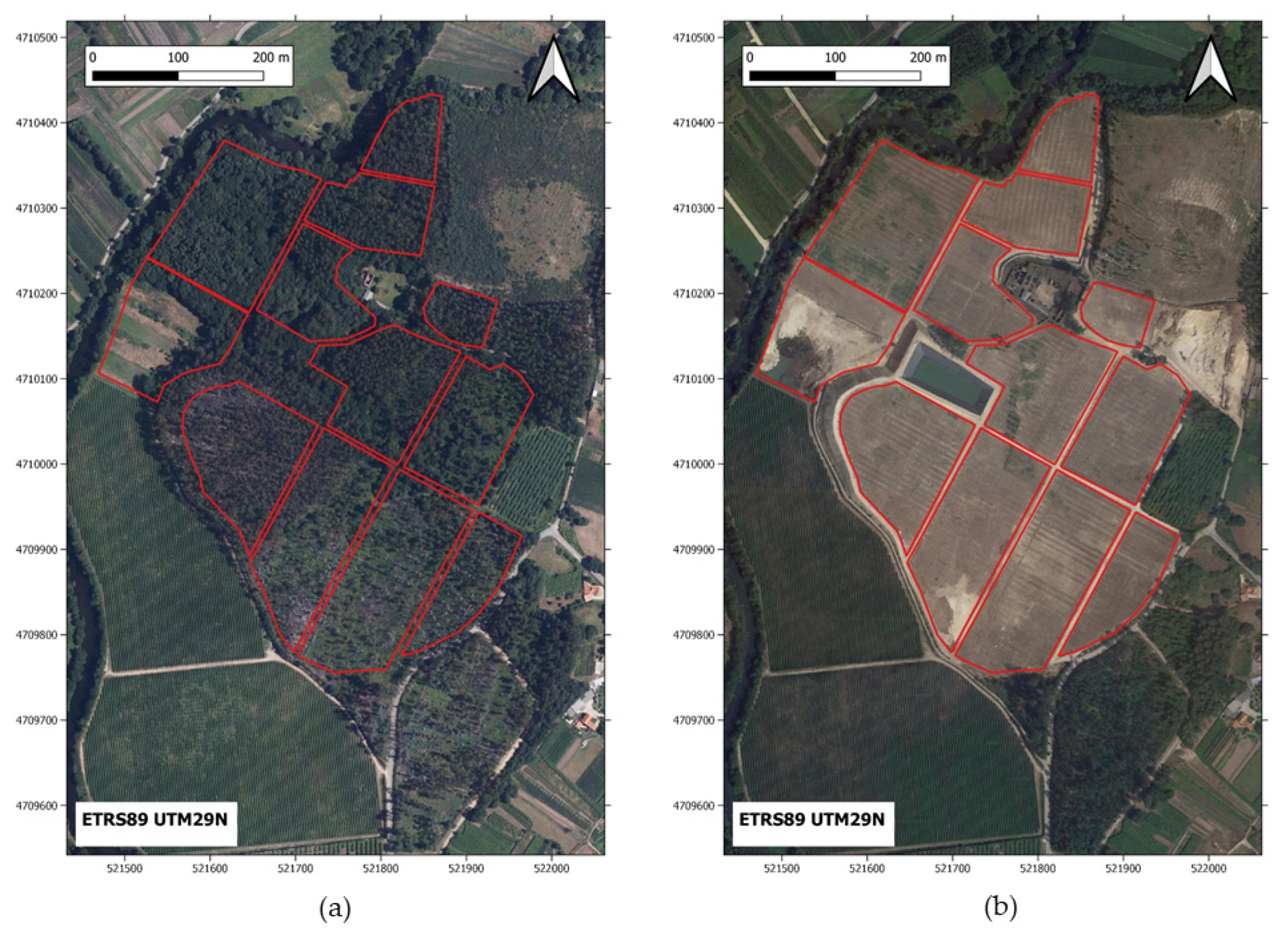
2.1. Description of the Study Site

The experiment was conducted in a newly planted vineyard located in Ribadumia in NW Spain (42°32′37.65″ N, 8°44′03.91″ W; 28 m above sea level), within the Rías Baixas DO. The total study area was 17.5 ha. The plantation was performed in 2018–2019 after finishing the land movements required for adapting the area prior to the design of the new vineyard (Figure 1). The zone closer to the river has been previously used for agricultural purposes, whereas the rest of the surface of this new vineyard has been devoted to forest for the last 20 years (Figure 1).
A fertigation system, using surface drip irrigation, was installed in 2019, allowing the application of water and nutrients through twelve irrigation sectors (Figure 1). Soil sample collection in this study was performed before the installation of the fertigation system. Climate at this site is Atlantic, with 14.3 °C of annual average temperature and 1432 mm of annual rainfall, as recorded in the nearest weather station (5 km) during the period from 2003 to 2017. The soil at this site is developed upon granite bedrocks and is classified as an Anthrosol [19].

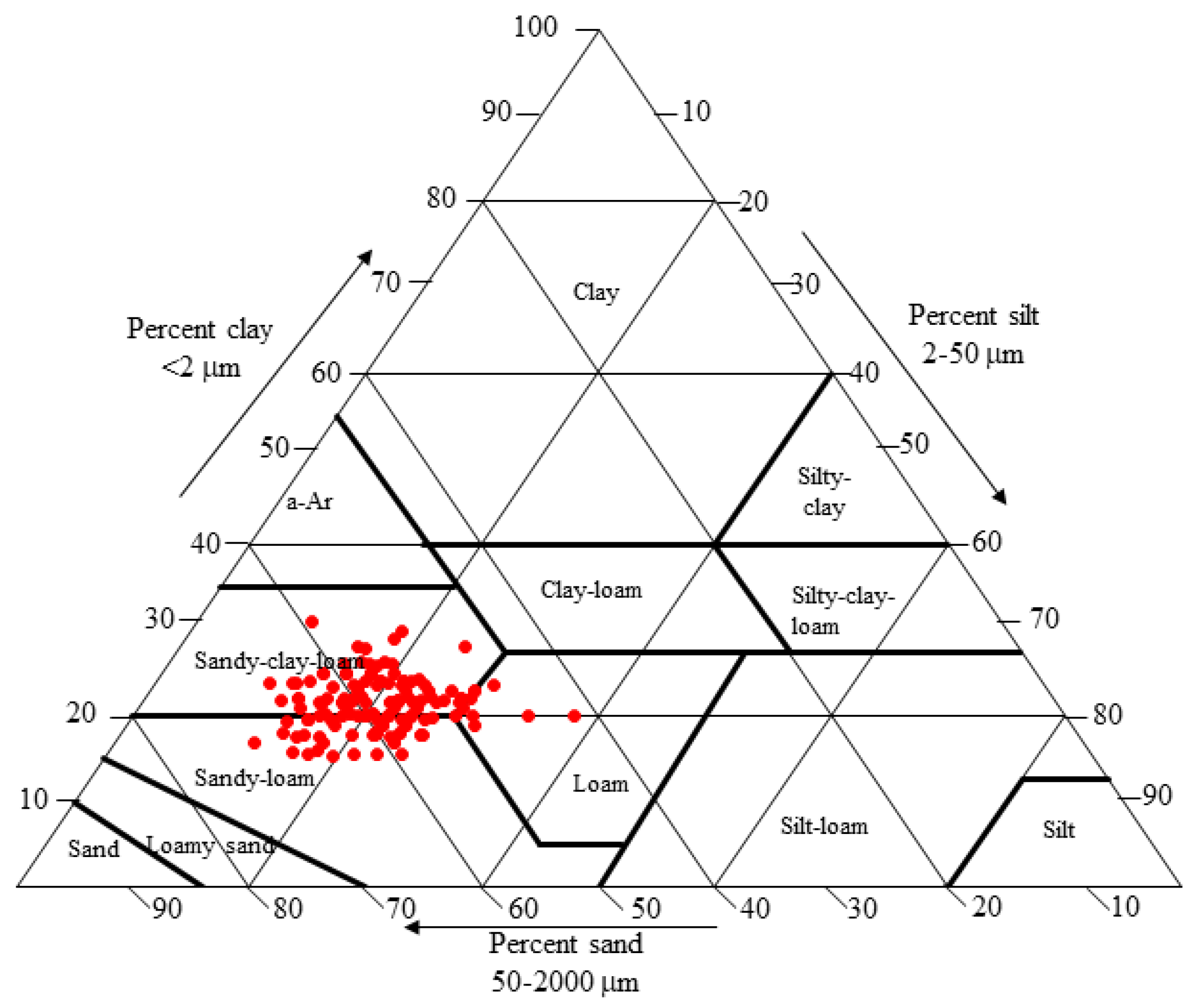
2.2. Soil Sampling and Analysis

Soil samples were taken from the surface horizon (0–40 cm depth) following a 35 × 35 m grid (n = 149) for physico-chemical analysis. Samples were air-dried and sieved to 2.00 mm. Soil physical and chemical properties were determined according to standard methods [20]. Particle size analysis (coarse and fine fractions as well as the contents in sand, silt and clay) was conducted after organic matter destruction with H2O2, elimination of Fe and Al oxihydroxides with HCl and dispersion with hexametaphosphate and sodium carbonate. Particles >50 mm were separated by wet sieving, while those <50 mm were separated through the pipette method. Soil pH was determined in water and 1 M KCl (soil: solution 1:2.5) using a pH-meter (Multimeter MM41, Crison, L’Hospitalet de Llobregat, Barcelona, Spain). Total organic carbon and nitrogen contents were measured with an elemental analyzer (TruSpec-CHNS, LECO Corporation, St. Joseph, MI, USA). From the content in organic carbon, the value of organic matter was computed. Exchangeable Ca, Mg, Na, K, Al and effective cation exchange capacity (ECEC) were determined following extraction with 1 M ammonium chloride, using atomic absorption and emission spectroscopy (Optima 4300 DV, Perkin Elmer, Boston, MA, USA) [21]. The ECEC was computed as the sum of Ca, Na, Mg, K and Al cations [22]. Available P was extracted in 0.5 M NaHCO3 and determined colorimetrically using UV-visible spectroscopy (Jenway 6300, Cole-Parmer Ltd., Staffordshire, UK) [23]. From these data, soil hydraulic properties (permanent wilting point, field capacity and soil water holding capacity) were calculated employing pedotransfer functions developed for soils of the region [24].
PWP = 0.376 × Clay + 6.39
FC = 0.33 × Clay + 0.15 × Silt + 1.54 × OC + 17.3
where: PWP is permanent wilting point (mm), Clay is the clay content (%), FC is field capacity (mm), Silt is silt content (%) and OC is the organic carbon content (%).
Apparent electrical conductivity (ECa) data were collected during the dry season using an electromagnetic induction sensor (EM-38DD, Geonics Ltd., Mississauga, ON, Canada). This device consists of a transmitter and a receiver coil installed 1.0 m apart at the opposite ends of a nonconductive bar. The system runs on a 9 V battery and operates at a frequency of 14.6 kHz. The obtained measurement is not only a function of the different conductivities in the subsoil but also of other factors such as the orientation (vertical or horizontal) of the coils, the operating frequency and the magnetic susceptibility. A comprehensive description of the EM-38 equipment can be found elsewhere [25].
The depth range of the measurements depends on the orientation of the coils. According to Heil and Schmidhalter [26], the sensitivity in the vertical mode is maximum at 40 cm below the instrument, while the sensitivity in the horizontal mode is the highest directly below the instrument. Usually, it is considered that the depth range is, respectively, 1.5 and 0.75 m when using the vertical or the horizontal dipole.
The EM-38 was transported manually over the vineyard. ECa measurements were made on 29 May 2020. The intensity of the collected data was 0.03 measurements m−2. The distance between transects was around 35 m. A global positioning system (GPS-RTK) was used to determine the geographical coordinates of the ECa measurements. In this research, two dipoles (vertical, ECa-V, and horizontal, ECa-H) of EM-38 were used. The interpolation of these measurements to obtain a continuous surface of the ECa over the vineyard was made by the regression kriging method [27].

2.3. Statistical Characterization of the Data

Several indicators, generally accepted for assessing central trend and data spread (mean, median, standard deviation, coefficient of variation (CV), minimum, maximum, skewness and kurtosis), were used for describing the data set. The Shapiro–Wilk test was used to determine whether or not data followed a normal distribution. The relationships between ECa (both ECa-H and ECa-V), topographic features (elevation and slope) and soil physico-chemical properties were assessed through the Spearman correlation coefficient, rho, in order to discern if ECa could be a useful ancillary variable for estimating the spatial distribution of soil properties through geostatistical interpolations. This coefficient was employed instead of that by Pearson because of the absence of normality in the dataset. Data were not transformed to normal distribution to avoid complex back transformations that often confer little benefit and, sometimes, exaggerate interpolation errors [28].

2.4. Geostatistical Analysis

Spatial variability was assessed through semivariogram calculation, graphing and model fitting for each soil property following the assumptions of stationarity in accordance with the intrinsic hypothesis [29,30]. Because of the limited number of data, the omnidirectional semivariogram was calculated, and spatial variability was assumed to be identical in all directions.
The following semivariogram parameters were defined: (a) nugget effect (C0), which is the value of the semivariogram when distance is 0; (b) range of spatial dependence (d), which is the distance at which a semivariogram remains approximately constant, after increasing with distance; (c) threshold (C0 + C1), which is the sill value approaching the data variance. In addition, the dependence ratio (DR) was computed [31]. The DR represents the percentage of the nugget effect in relation to the sill. The values of this ratio can be ranked as follows: strong (<25%), moderate (25%–75%) and weak dependence (>75%). Furthermore, the mean correlation distance (MCD) was calculated to estimate the distance over which the data have a high spatial dependence [32].
Model performance was checked through the leave-one-out cross-validation technique [33]. Three criteria were used to determine the goodness-of-fit of the models [34]: (a) the coefficient of correlation (r) between measured and estimated values; (b) the mean error (ME); and (c) the mean square prediction error (MSPE). For an unbiased prediction, centered on the true values, ME and MSPE should be close to zero.
Geostatistical interpolation of the soil properties over the experimental vineyard was performed using ordinary kriging (OK). This is a standard technique for spatial interpolation and provides each cell with a local, optimal prediction and an estimation of the error that depends on the semivariogram and the spatial configuration of the data [35]. The OK weights minimize the variance of the estimation [29].
The calculation of the semivariograms and the spatial distribution of the measured soil properties over the experimental vineyard was performed through OK using the gstat package [36,37] for the R v3.6.2 environment [38].

3. Results

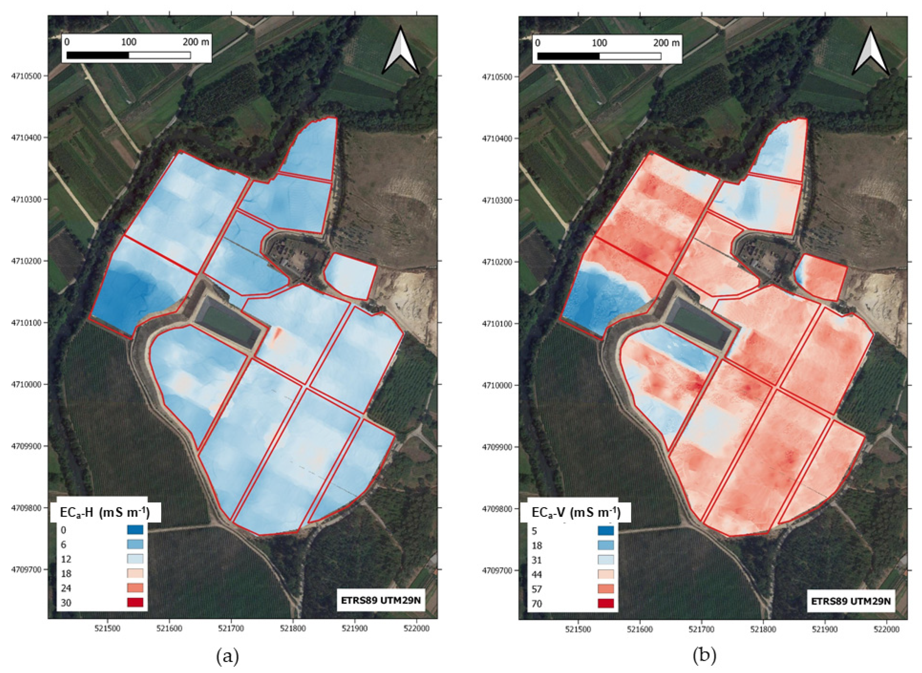
3.1. Statistical Characterization of Soil Properties in the Experimental Vineyard

In the studied vineyard, soil was acid and pH in water averaged 5.1, whereas pH in KCl was 4.35 on average. Both pH in water and in KCl showed a low variability, with CV values of 6.3% and 4.2%, respectively (Table 1). The components of the exchange complex showed a high spatial variability within the experimental vineyard, and their CV values ranged from 32.9% for aluminum to 105.2% for calcium (Table 1). In contrast, the variability of the ECEC was lower (CV = 23.7%), ranging from 1.84 to 7.0 cmol(+) kg−1 (Table 1). As expected in acid soils, the content of aluminum at saturation was high on average (63.28%), although it oscillated between 4.81% and 88.54%.
In the studied vineyard, P content averaged 11.67 mg kg−1, although ranging from 3.34 to 25.73 mg kg−1, showing a moderately high CV of 45.2% (Table 1). Organic matter ranged from 1.28% to 7.96%, and averaged 3.88%, presenting a relatively high CV (35.6%). On average, soil carbon content was moderately high (2.25%), ranging from 0.74% to 4.62%; whereas nitrogen content varied between 0.04% and 0.41% (Table 1). This led to a similar CV, around 35%, for both C and N contents. The C/N ratio varied between 9.71 and 29.47. Soil samples in the studied vineyard presented loam, sandy-loam and clay-sandy-loam textures (Figure 2). The CV of the sand, silt and clay fractions was 8.4%, 23.1% and 14.1%, respectively (Table 1). Soil water holding capacity over the study vineyard varied between 128.8 and 228.0 mm m−1, showing a low CV, less than 10% (Table 1).
Concerning the ECa measurements, a buffer area of 5 m diameter around each soil sample location was built using a geographical information system (QGIS v3.8, https://qgis.org). Figure 3 displays the ECa maps for both the horizontal (ECa-H) and vertical (ECa-V) dipoles. The ECa-H map is rather homogeneous, although an area with values close to 1 mS m−1 is clearly observed. The ECa-V shows a high spatial variability, with areas in which ECa is less than 10 mS m−1 while most of the vineyard soil had ECa greater than 45 mS m−1. From the ECa (vertical and horizontal dipoles) measurements and topographical parameter maps, and considering the buffer areas, median, minimum and maximum values were extracted from these maps. In the case of the horizontal dipole, ECa was about 10 mS m−1, whereas in the case of the vertical dipole, ECa values were around 45 mS m−1 (Table 1).
Means and medians of the studied properties were rather similar; however, skewness and kurtosis coefficients were highly variable (Table 1). Shapiro–Wilk’s test confirmed the absence of normality in the data distributions for all properties, with the exception of sand content, and fine and coarse fractions (data not shown). Despite this, data were not transformed for conducting the geostatistical analysis.
Correlation coefficients between ECa and the measured soil properties were low, although significant in some cases such as the pairs: K/ECa-H min (rho = −0.222; p-value = 0.007), fine fraction/ECa-V max (rho = 0.295; p-value < 0.001) or ECEC/ECa-H min (rho = −0.228; p-value = 0.005). Topographical features (elevation and slope) showed weak correlations with soil attributes, being Na/elevation (rho = −0.495; p-value < 0.001), P/elevation (rho = −0.377; p-value < 0.001) and coarse fraction/slope (rho = 0.265; p-value = 0.001) the pairs with the strongest correlation coefficients. The Spearman correlation coefficients between soil water retention capacity and ECa measurements were negative and did not surpass 0.18. Due to these weak correlations, ECa and topographical features were not used as ancillary information for improving ordinary kriging interpolations of soil properties.

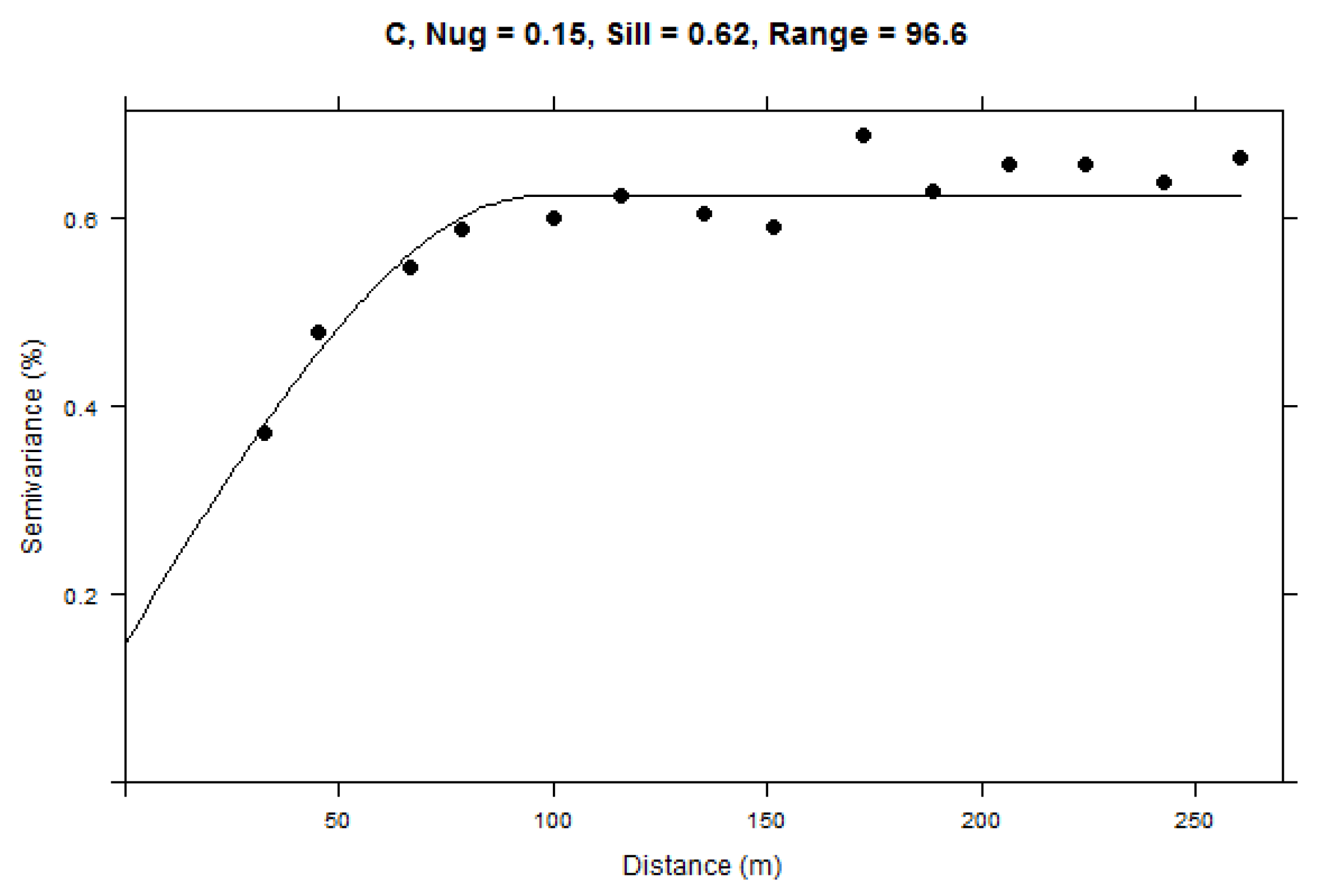
3.2. Spatial Dependence Analysis

Spatial dependence was observed in all soil properties except for Ca content and the C/N ratio, which did not show a spatial structure and were modelled by a pure nugget effect (Table 2). Spherical functions with variable nugget effects depending on the analyzed soil property were fitted to experimental data (Table 2). In the case of Mg and Na, the nugget effect was nul. As an example, the experimental semivariogram of soil C content and its fitted model are shown in Figure 4.
The range of the fitted models varied between 29.6 (Aluminum at saturation) and 287.5 m (P content). Ranges were lower than 50 m on 2 occasions, between 50 and 100 m in 9 cases and higher than 100 m 13 times (Table 2). Due to this short spatial dependence range, kriging interpolation results showed high kriging estimation errors as the distance to the sampling point increased.
Most soil properties presented a strong spatial dependence since DR values were less than or equal to 25% in 11 of the properties studied; a moderate dependence was observed for 11 soil properties, whereas a weak spatial dependence was observed only for ECEC (Table 2). The MCD values confirmed these outcomes, and pH in water, soil P content and ECa were over the distance among nodes of the sampling grid (35 m), whereas the rest of the soil properties considered showed smaller MCD values (Table 2).
Cross-validation indicators showed that, in most cases, the theoretical structures adequately described the spatial dependence of the studied soil properties (Table 2). Mean error was close to the value considered a good fit in all cases, except for aluminum at saturation, fine and coarse fractions, sand content, and ECa-V (both median, max and min) (Table 2). In contrast, MSPE values were far from the optimal threshold for a good fit in most cases (Table 2). Correlation coefficients between measured and predicted values varied between 0.30 and 0.77, depending on the soil property considered (Table 2). Higher values were observed for ECa, suggesting a greater homogeneity for this variable.

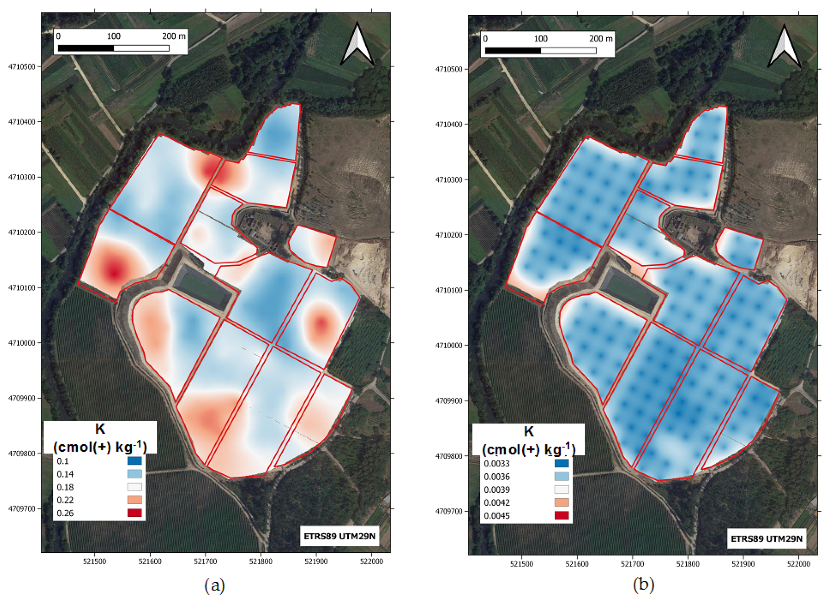
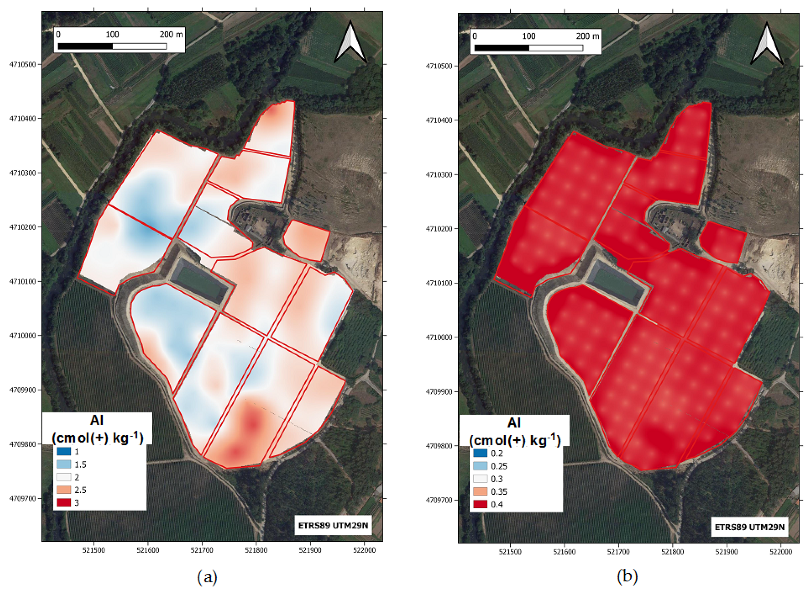
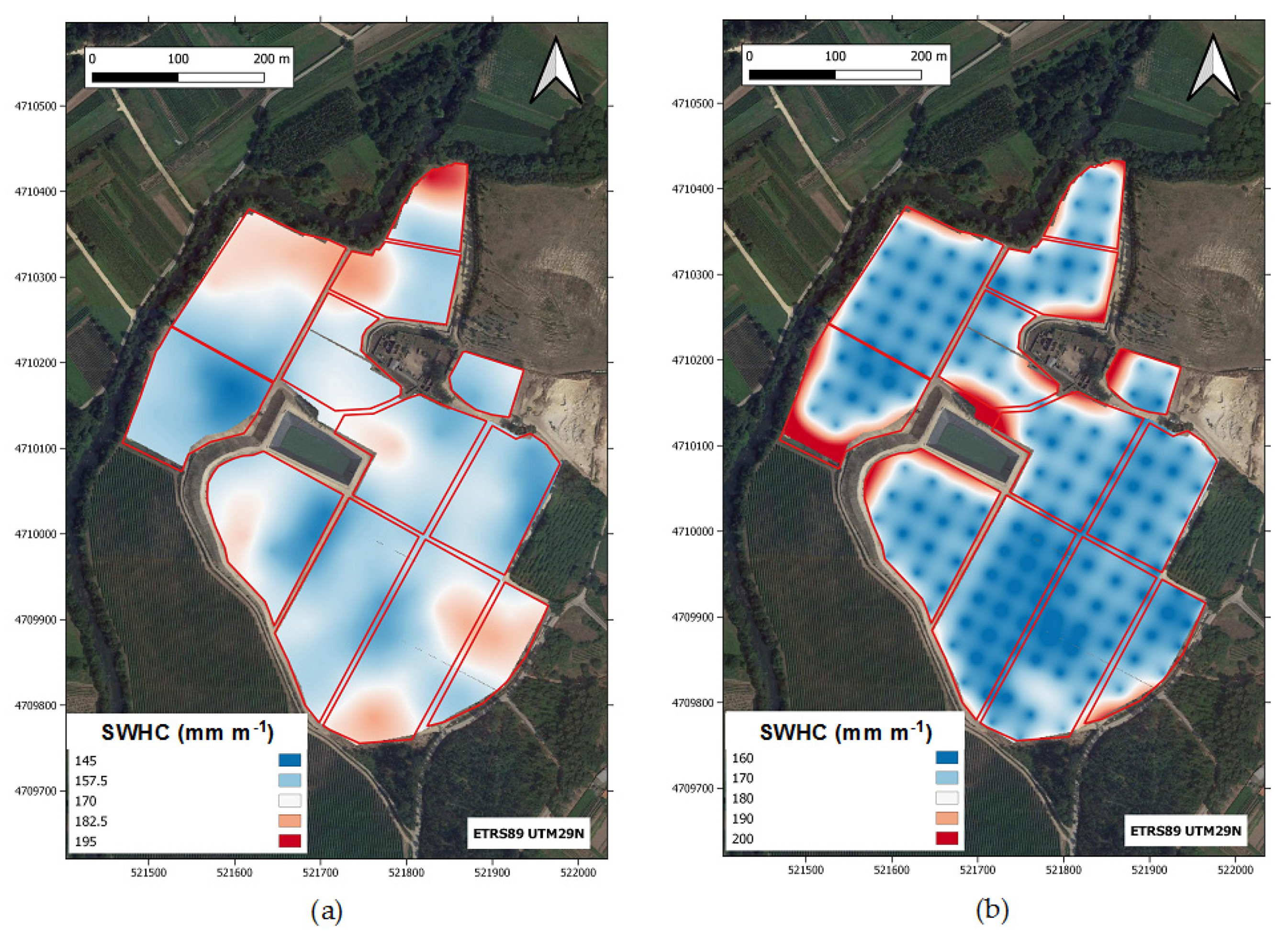
3.3. Kriging Interpolation

Ordinary kriging interpolation allowed for obtaining smooth surface maps of the determined soil properties, showing, in general, high and uniform uncertainty patterns; namely, errors were high in most of the study area except close to the sampling points. However, due to the low ME and MSPE values obtained in the cross-validation, OK produced useful maps for several soil properties including pH, clay content, soil water holding capacity, ECEC, organic matter, C, K, N, Na and Mg. In the case of pH in water (Figure 5a), a smooth surface with smaller values (between 4.6 and 4.8) in the area close to the river and in the middle of the vineyard was produced. A small area with pH close to 5.5 was observed. Moreover, interpolation errors were low (less than 0.08) in most of the vineyard area (Figure 5b).
Soil C content map obtained through OK (Figure 6a) shows a more heterogenous pattern than that for pH. Soil C contents were low (less than 2%) near the river and greater than 3.5% in some areas located far from the river, although patches of high and low soil C contents were estimated all over the vineyard surface. The estimation error map displayed a uniform pattern, with low values (less than 0.35%) for almost the entire vineyard surface (Figure 6b). Soil organic matter showed an equal distribution pattern to that of C in the studied vineyard.
The estimation map for ECEC displayed an area, in the center of the vineyard, with values lower than 3.2 cmol(+) kg−1, while some patches with higher values (up to 4.4 cmol(+) kg−1) were estimated in the south part of the vineyard (Figure 7a). The estimation error map displayed a uniform pattern, with low values (less than 0.55 cmol(+) kg−1) for almost the entire vineyard surface (Figure 7b). It must be noted that the maps for soil C content and ECEC showed a certain resemblance to those maps of ECa due to the significant, although weak (rho between −0.15 and −0.22), correlation among these variables.
Figure 8a shows the OK maps for clay content. The estimation map shows a clear pattern with clay contents lower than 20% in the central part of the vineyard and values higher than 23% in the extremes (East and West areas). The estimation error map displayed a uniform pattern, with errors lower than 8% for almost the entire vineyard surface (Figure 8b). A certain resemblance between the estimation map of clay content and the ECa maps must be noted.
The estimation map for K displayed areas, mainly in the center of the vineyard, with values lower than 0.15 cmol(+) kg−1, while some areas with higher values (up to 0.26 cmol(+) kg−1) were also estimated (Figure 9a). The estimation error map displayed a uniform pattern, with low values (less than 0.0035 cmol(+) kg−1) for almost the entire vineyard surface (Figure 9b). It must be noted that the map of K showed a certain resemblance to those maps of ECa due to the significant, although weak (rho between −0.14 and −0.22; p-values ranging between 0.006 and 0.071), correlation among these variables.
The estimation map for Al displayed areas with values lower than 1.5 cmol(+) kg−1, close to the river; while some areas with high values (up to 3 cmol(+) kg−1) were estimated in the South of the vineyard (Figure 10a). The estimation error map displayed a uniform pattern, with high values (approximately 0.4 cmol(+) kg−1) for almost the entire vineyard surface (Figure 10b).
The estimation map for soil water holding capacity displayed areas with values greater than 190 mm m−1, while some areas with values lower than 150 mm m−1 were also estimated, mainly in the surroundings of the water reservoir for irrigation (Figure 11a). The estimation error map displayed a uniform pattern, with very high values (more than 150 mm m−1) for almost the entire vineyard surface (Figure 11b). No clear resemblance between the map of soil water holding capacity and those maps of ECa was observed, likely due to the weak and not significant (rho between −0.06 and −0.18; p-value > 0.05) correlation among these variables. Despite this, high ECa measurements (Figure 1) tended to occur in areas of the vineyard with low water holding capacities.

4. Discussion

The current study characterized the soil in a newly established vineyard and statistical indicators showed that most of the soil properties determined in the experimental vineyard had a high spatial variability, suggesting the convenience of site-specific management [39]. Soil texture in the studied vineyard varied from sandy-loam to clay-sandy-loam, with a fine fraction greater than 60% on average. When comparing the nutrient contents of the studied soil with those considered optimal [40], important deficits are detected for Ca, Mg and K, as well as unbalances for the K/Mg ratio over the whole vineyard. In contrast, organic matter was close to the optimal values for acid soils. However, nitrogen contents vary from very low to very high within the experimental vineyard. In view of these results, a uniform management of fertilization could lead to over- and under-fertilized zones over this vineyard, as reported in other studies [41], leading to a wide heterogeneity in vine development [16] and grape composition [4].
The spatial variability of the determined soil properties was characterized by spherical structures, in contrast to the most common exponential models [42,43]. In the current study, all soil attributes showed a pattern of spatial dependence except for Ca and C/N ratio. As shown in Table 2, the experimental semivariograms were best fitted to theoretical models without nugget effect only on 2 occasions (Mg and Na) and by a nugget effect plus a structure in the remaining datasets. Range values of the theoretical structures varied between 29.6 and 245.9 m. This fact might not only have consequences in kriging interpolations, but also, it could be pointing to the need for a denser sampling grid to capture the spatial variability patterns of all the variables over the experimental vineyard. In fact, it is well-known that the sampling network has a major role in the spatial dependence structure [35].
The current study was carried out in a nonsaline area of the humid zone of Europe; therefore, ECa measurements were not affected by salts, and so they might be useful for assessing other soil properties and to delineate zones within the experimental vineyard, as reported in previous studies carried out in nonsaline areas [27,44,45]. Despite being significant on some occasions, correlation coefficients among ECa and soil properties were low (never greater than 0.27) and, usually, negative. In nonsaline soils, significant correlations between ECa and soil texture are common [46]; however, in the current study, the correlation coefficients between ECa and sand, silt and clay contents were less than 0.1 for the vertical dipole and less than 0.2 for the horizontal dipole. This contrasts with the observations made on a grassland area in the same region of NW Spain [43], where significant correlations were detected between ECa and soil textural fractions, with correlation coefficients up to 0.48 for the case of sand. This points out the fact that the relationships between a given soil property and ECa might be site-specific and have to be determined on a field-by-field basis [10]. This site-specificity of the relationships between ECa measurements and soil properties can be explained by (i) the complex interaction of soil properties, (ii) a temporal component of variability that is weakly reflected by an expected constant variable such as the ECa and (iii) variable climatic factors [26,47]. Despite the lower correlation coefficients observed between ECa and soil textural fractions, the spatial variability patterns of both variables within the studied vineyard had a reasonable similarity, especially for clay and fine and coarse fractions, which makes them useful for delineating zones with similar soil texture.
Since no direct measurements of soil hydrologic properties could be performed, we employed data on texture and organic matter content to estimate soil water holding capacity through statistical correlations among these variables, which are known to provide sufficiently accurate estimates for taking decisions [48]. The equations employed were developed for a wide representation of soils from NW Spain [24], in order to reduce the discrepancies often reported for the use of this methodology [48,49]. In fact, a comparative study on several pedotransfer functions reported that the efficiency of these methods is highly variable [50]. However, despite the uncertainties regarding the accuracy of the estimates obtained, the soil water holding capacity map could provide relevant information for planning irrigation since it was able to capture the spatial variability of this property over the vineyard.
Furthermore, other soil properties showed spatial variability patterns similar to those of ECa in the studied vineyard, despite the low correlation coefficients detected among soil attributes. In particular, the soil properties with the most similar spatial patterns to those of ECa were the following: pH in water, C and N contents, ECEC (including its components, K, Mg and Na), available P and aluminum at saturation. Previous works in NW Spain reported a correspondence between ECa and soil organic matter maps [22]; however, this relationship seemed to be noncausal [51,52]. This can be extended to the rest of the soil properties determined in the current study. Rodríguez-Pérez et al. [53] did not find significant relations between ECa measurements and extractable potassium contents; meanwhile, K/ECa-H relations were significant in our study, pointing out the fact that the relationships between ECa and soil properties are highly variable [10] and, when significant, ECa has been reported useful for providing secondary information that allows for enhancing the interpolations [54]. Unfortunately, weak correlations were detected in the current study, and ECa could not be used as an ancillary variable for improving the maps of soil chemical properties. It must be taken into account that the soil in the vineyard is anthropic (land movements were required), and an organic soil layer was used to fill the original soil, so the ECa measurements were able to indicate that the subsoil is not homogeneous over the vineyard. The zone closer to the river, with lower ECa values, had been previously used for agricultural purposes, whereas the rest of the surface of this new vineyard had been devoted to forest for the last 20 years (as depicted in Figure 1).
The low correlation coefficients observed in the current study pointed out that the sampling grid should have been denser in order to capture possible correlations between ECa measurements and the determined soil properties, in accordance with the outputs of the spatial dependence analysis. This reduces the capacity of ECa measurements to obtain quantitative information of soil chemical properties; however, advantages over traditional methods, such as ease of use and low cost, being less invasive and allowing a high volume of data to be collected, make this technique a very useful approach for mapping soils and aiding in delineating management zones [55]. Nevertheless, the maps resulting from the current study may help to develop fertilization practices adapted to the spatial variability of soil chemical properties within the studied vineyard, allowing for site-specific management depending on the spatial distribution of soil nutrients (N, P, K and Mg). The fertigation system installed in this vineyard would allow for a differential supply of nutrients to each of the sectors, according to the results obtained in the current study regarding ECa and soil chemical properties. Furthermore, ECa can allow for a low-cost monitoring of the evolution of the nutrient contents in the soil, supported by a reduced soil sampling following an irregular grid that would enhance the correlations between this indirect measurement and the soil chemical properties.
Finally, the studied vineyard will face several limitations that include the lack of nutrients typical in granite-derived soils, reflected in the low ECEC, and insufficient soil water holding capacity due to low clay contents and high Al mobility that may be toxic to grapevines. The information derived from the current study provides a basis for making decisions on the management techniques to apply in order to cope with the aforementioned limitations and favor the expression of the terroir in the wines produced [56].

5. Conclusions

Since a vineyard has an estimated lifespan of 20–40 years, decisions made in its establishment are crucial for its sustainability in the future. The current study indicates that soil characterization is essential for delineating site-specific management zones in a newly planted vineyard. Using ECa as a noninvasive technique might provide useful information for vineyard zoning at acceptable costs to be obtained. Overall, the studied vineyard showed low contents in essential nutrients (Ca, K, Mg and P), so they must be applied differently according to the zones defined by the maps obtained in the current study. The balances among antagonist nutrients must be considered. Actual irrigation sectors are not coincident with the spatial variability detected for soil water holding capacity and ECa, consequently, vineyard owners must make adaptations in order to carry out an efficient irrigation (or fertigation), accounting for the variability detected in the study plot.

Author Contributions

Conceptualization, J.D. and J.J.C.; methodology, J.D., J.J.C. and J.M.M.-A.; validation, J.M.M.-A., M.F., J.D. and J.J.C.; formal analysis, J.D. and J.M.M.-A.; investigation, J.M.M.-A., M.F., J.D. and J.J.C.; resources, J.J.C.; data curation, J.D. and J.M.M.-A.; writing—original draft preparation, J.M.M.-A.; writing—review and editing, J.M.M.-A., M.F., B.J.R., J.D. and J.J.C.; supervision, B.J.R., J.D. and J.J.C.; project administration, J.J.C.; funding acquisition, J.J.C. All authors have read and agreed to the published version of the manuscript.

Funding

This research received no external funding.

Acknowledgments

Authors express their gratitude to Zamora Company for allowing the use of their newly-planted vineyard to carry out the current study. Authors would like to thank the use of Riaidt-USC-Campus Lugo analytical facilities.

Conflicts of Interest

The authors declare no conflict of interest.

References

  1. Mulla, D.J.; McBratney, A.B. Soil spatial variability. In Soil Physics Companion; Warrick, A.W., Ed.; CRC Press: Boca Ratón, FL, USA, 2002; pp. 343–373. [Google Scholar]
  2. Corá, J.E.; Araujo, A.V.; Pereira, G.T.; Beraldo, J.M.G. Variabilidade espacial de atributos do solo para adoção do sistema de agricultura de precisão na cultura de cana-de-açúcar. Rev. Bras. Cienc. Solo 2004, 28, 1013–1021. [Google Scholar] [CrossRef]
  3. Bramley, R.G.V.; Ouzman, J.; Boss, P.K. Variation in vine vigour, grape yield and vineyard soils and topography as indicators of variation in the chemical composition of grapes, wine and wine sensory attributes. Aust. J. Grape Wine Res. 2011, 17, 217–229. [Google Scholar] [CrossRef]
  4. Baluja, J.; Tardaguila, J.; Ayestaran, B.; Diago, M.P. Spatial variability of grape composition in a Tempranillo (Vitis vinifera L.) vineyard over a 3-year survey. Precis. Agric. 2013, 14, 40–58. [Google Scholar] [CrossRef] [Green Version]
  5. Vaudour, E.; Shaw, A.B. A worldwide perspective on viticultural zoning. S. Afr. J. Enol. Vitic. 2005, 26, 106–115. [Google Scholar] [CrossRef] [Green Version]
  6. Cancela, J.J.; Fandiño, M.; Rey, B.J.; Dafonte, J.; González, X.P. Discrimination of irrigation water management effects in pergola trellis system vineyards using a vegetation and soil index. Agric. Water Manag. 2017, 183, 70–77. [Google Scholar] [CrossRef]
  7. Arno, J.; Martínez-Casasnovas, J.A.; Ribes-Dasi, M.; Rosell, J.R. Review: Precision viticulture. Research topics, challenges and opportunities in site-specific vineyard management. Span. J. Agric. Res. 2009, 7, 779–790. [Google Scholar] [CrossRef] [Green Version]
  8. Santesteban, L.G.; Guillaume, S.; Royo, J.B.; Tisseyre, B. Are precision agriculture tools and methods relevant at the whole-vineyard scale? Precis. Agric. 2013, 14, 2–17. [Google Scholar] [CrossRef] [Green Version]
  9. Miller, B.A.; Koszinski, S.; Wehrhan, M.; Sommer, M. Comparison of spatial association approaches for landscape mapping of soil organic carbon stocks. Soil 2015, 1, 217–233. [Google Scholar] [CrossRef] [Green Version]
  10. Brevik, E.C.; Calzolari, C.; Miller, B.A.; Pereira, P.; Kabala, C.; Baumgarten, A.; Jordán, A. Soil mapping, classification, and pedologic modeling: History and future directions. Geoderma 2016, 264, 256–274. [Google Scholar] [CrossRef]
  11. Rhoades, J.D.; Chanduvi, F.; Lesch, S.M. Soil Salinity Assessment: Methods and Interpretation of Electrical Conductivity Measurements; FAO Irrigation and Drainage Paper 57; FAO: Rome, Italy, 1999. [Google Scholar]
  12. Vitharana, U.W.A.; van Meirvenne, M.; Cockx, L.; Bourgeois, J. Identifying potential management zones in a layered soil using several sources of ancillary information. Soil Use Manag. 2006, 22, 405–413. [Google Scholar] [CrossRef]
  13. Harvey, O.R.; Morgan, C.L.S. Predicting regional-scale soil variability using single calibrated apparent soil electrical conductivity model. Soil Sci. Soc. Am. J. 2009, 73, 164–169. [Google Scholar] [CrossRef]
  14. Bramley, R.G.V.; Proffitt, A.P.B.; Corner, R.J.; Evans, T.D. Variation in grape yield and soil depth in two contrasting Australian vineyards. In Soil 2000—New Horizons for a New Century, Australian & New Zealand 2nd Joint Soils Conference, 2: Oral Papers; Lincoln University, New Zealand, December 2000; Adams, J.A., Metherell, A.K., Eds.; New Zealand Society of Soil Science: Canterbury, New Zealand, 2000; pp. 29–30. [Google Scholar]
  15. Morari, F.; Castrignanò, A.; Pagliarin, C. Application of multivariate geostatistics in delineating management zones within a gravelly vineyard using geo-electrical sensors. Comput. Electron. Agric. 2009, 68, 97–107. [Google Scholar] [CrossRef]
  16. Fulton, A.; Schwankl, L.; Lynn, K.; Lampinen, B.; Edstrom, J.; Prichard, T. Using EM and VERIS technology to assess land suitability for orchard and vineyard development. Irrig. Sci. 2011, 29, 497–512. [Google Scholar] [CrossRef] [Green Version]
  17. Priori, S.; Martini, E.; Andrenelli, M.C.; Magini, S.; Agnelli, A.E.; Bucelli, P.; Biagi, M.; Pellegrini, S.; Constantini, E.A.C. Improving wine quality through harvest zoning and combined use of remote and soil proximal sensing. Soil Sci. Soc. Am. J. 2013, 77, 1338–1348. [Google Scholar] [CrossRef]
  18. Urretavizcaya, I.; Royo, J.B.; Miranda, C.; Tisseyre, B.; Guillaume, S.; Santesteban, L.G. Relevance of sink-size estimation for within-field zone delineation in vineyards. Precis. Agric. 2017, 18, 133–144. [Google Scholar] [CrossRef] [Green Version]
  19. IUSS Working Group WRB. World Reference Base for Soil Resources 2014, Update 2015. International Soil Classification System for Naming Soils and Creating Legends for Soil Maps. World Soil Resources Reports No. 106; FAO: Rome, Italy, 2015; p. 192. [Google Scholar]
  20. Tan, K.H. Soil Sampling, Preparation, and Analysis; Marcel Dekker: New York, NY, USA, 1996. [Google Scholar]
  21. Sumner, M.E.; Miller, W.P. Cation exchange capacity and Exchange coefficients. In Methods of Soil Analysis Part 3 Chemical Methods; American Society of Agronomy: Madison, WI, USA, 1996; pp. 437–474. [Google Scholar]
  22. Kamprath, E.J. Exchangeable aluminium as a criterion for liming leached mineral soils. Soil Sci. Soc. Am. J. 1970, 34, 252–254. [Google Scholar] [CrossRef]
  23. Olsen, S.R.; Sommers, L.E. Phosphorus. In Methods of Soil Analysis Part 2 Chemical and Microbiological Properties; American Socitey of Agronomy: Madison, WI, USA, 1982; pp. 403–430. [Google Scholar]
  24. Soto, B.; Arias, M.; Díaz-Fierros, F. Desarrollo de una función de pedotransferencia para los suelos de Galicia (NW Spain). Agrochimica 2001, 45, 178–188. [Google Scholar]
  25. Corwin, D.L.; Lesch, S.M. Characterizing soil spatial variability with apparent soil electrical conductivity: Part I. Survey protocols. Comput. Electron. Agric. 2005, 46, 103–133. [Google Scholar] [CrossRef]
  26. Heil, K.; Schmidhalter, U. Characterisation of soil texture variability using the apparent soil electrical conductivity at a highly variable site. Comput. Geosci. 2012, 39, 98–110. [Google Scholar] [CrossRef]
  27. García-Tomillo, A.; Mirás-Avalos, J.M.; Dafonte-Dafonte, J.; Paz-González, A. Estimating soil organic matter using interpolation methods with a electromagnetic induction sensor and topographic parameters: A case study in a humid region. Precis. Agric. 2017, 18, 882–897. [Google Scholar] [CrossRef]
  28. Robinson, T.P.; Metternicht, G. Testing the performance of spatial interpolation techniques for mapping soil properties. Comput. Electron. Agric. 2006, 50, 97–108. [Google Scholar] [CrossRef]
  29. Goovaerts, P. Geostatistical approaches for incorporating elevation into the spatial interpolation of rainfall. J. Hydrol. 2000, 228, 113–129. [Google Scholar] [CrossRef]
  30. Vieira, S.R. Uso de geoestatística em estudos de variabilidade espacial de propriedades do solo. In Tópicos em Ciência do Solo; Novais, R.F., Ed.; Sociedade Brasileira da Ciência do Solo: Viçosa, Brazil, 2000; pp. 3–87. [Google Scholar]
  31. Cambardella, C.A.; Moorman, T.B.; Novak, J.M.; Parkin, T.B.; Karlen, D.L.; Turco, R.F.; Konopka, A.E. Field-scale variability of soil properties in central Iowa soils. Soil Sci. Soc. Am. J. 1994, 58, 1501–1508. [Google Scholar] [CrossRef]
  32. Han, S.; Evans, R.G.; Schneider, S.M.; Rawlins, S.L. Spatial variability of soil properties on two-center pivot irrigated fields. In Proceedings of the Third International Conference on Precision Agriculture, Minneapolis, MN, USA, 23–26 June 1996; American Society of Agronomists: Madison, WI, USA, 1996; pp. 97–106. [Google Scholar]
  33. Chilés, J.P.; Delfiner, P. Geostatistics. Modelling Spatial Uncertainty; Wiley: New York, NY, USA, 1999. [Google Scholar]
  34. Karnieli, A. Application of kriging technique to areal precipitation mapping in Arizona. GeoJournal 1990, 22, 391–398. [Google Scholar] [CrossRef]
  35. Goovaerts, P. Geostatistics for Natural Resources Evaluation; Applied Geostatistics Series; Oxford University Press: Oxford, UK, 1997. [Google Scholar]
  36. Pebesma, E.J. Multivariable geostatistics in S: The gstat package. Comp. Geosci. 2004, 30, 683–691. [Google Scholar] [CrossRef]
  37. Gräler, B.; Pebesma, E.J.; Heuvelink, G. Spatio-temporal interpolation using gstat. RFID J. 2016, 8, 204–218. [Google Scholar] [CrossRef]
  38. R Core Team. R: A Language and Environment for Statistical Computing; R Foundation for Statistical Computing: Vienna, Austria, 2019; Available online: https://www.R-project.org/ (accessed on 4 July 2020).
  39. Moral, F.J.; Terrón, J.M.; Marques da Silva, J.R. Delineation of management zones using mobile measurements of soil apparent electrical conductivity and multivariate geostatistical techniques. Soil Till. Res. 2010, 106, 335–343. [Google Scholar] [CrossRef]
  40. Hazelton, P.; Murphy, B. Interpreting Soil Test Results. What Do All the Numbers Mean? CSIRO Publishing: Clayton, Australia, 2007. [Google Scholar]
  41. Roy, S.K.; Shibusawa, S.; Okayama, T. Textural analysis of soil images to quantify and characterize the spatial variation of soil properties using a real-time soil sensor. Precis. Agric. 2006, 7, 419–436. [Google Scholar] [CrossRef]
  42. Bonnin, J.J.; Mirás-Avalos, J.M.; Lanças, K.P.; Paz González, A.; Vieira, S.R. Spatial variability of soil penetration resístanse influenced by season of sampling. Bragantia 2010, 69, 163–173. [Google Scholar] [CrossRef]
  43. García-Tomillo, A.; Mirás-Avalos, J.M.; Dafonte-Dafonte, J.; Paz-González, A. Mapping soil texture using geostatistical interpolation combined with electromagnetic induction measurements. Soil Sci. 2017, 182, 278–284. [Google Scholar] [CrossRef]
  44. Farahani, H.J.; Buchleiter, G.W.; Brodahl, M.K. Characterization of apparent soil electrical conductivity variability in irrigated sandy and non-saline fields in Colorado. Trans. ASAE 2005, 48, 155–168. [Google Scholar] [CrossRef]
  45. Gozdowski, D.; Stępień, M.; Samborski, S.; Dobers, E.S.; Szatyłowicz, J.; Chormański, J. Prediction accuracy of selected spatial interpolation methods for soil texture at farm field scale. J. Soil Sci. Plant Nutr. 2015, 15, 639–650. [Google Scholar] [CrossRef] [Green Version]
  46. Sudduth, K.; Drummond, S.; Kitchen, N. Accuracy issues in electromagnetic induction sensing of electrical conductivity for precision agriculture. Comput. Electron. Agric. 2001, 31, 239–264. [Google Scholar] [CrossRef]
  47. Corwin, D.L.; Lesch, S.M. Characterizing soil spatial variability with apparent soil electrical conductivity. Part II. Case study. Comput. Electron. Agric. 2005, 46, 135–152. [Google Scholar] [CrossRef]
  48. Saxton, K.E.; Rawls, W.J. Soil water characteristic estimates by texture and organic matter for hydrologic solutions. Soil Sci. Soc. Am. J. 2006, 70, 1569–1578. [Google Scholar] [CrossRef] [Green Version]
  49. Gijsman, A.J.; Jagtap, S.S.; Jones, J.W. Wading through a swamp of complete confusion: How to choose a method for estimating soil water retention parameters for crop models. Eur. J. Agron. 2002, 18, 75–105. [Google Scholar] [CrossRef]
  50. Martínez, E.M.; Serafín Cuesta, T.; Cancela, J.J. The efficiency of different estimation methods of hydro-physical limits. Rev. Bras. Ciênc. Solo 2012, 36, 1756–1768. [Google Scholar] [CrossRef] [Green Version]
  51. Tarr, A.; Moore, K.J.; Burras, C.L.; Bullock, D.G.; Dixon, P.M. Improving map accuracy of soil variables using soil electrical conductivity as a covariate. Precis. Agric. 2005, 6, 255–270. [Google Scholar] [CrossRef] [Green Version]
  52. Peralta, N.R.; Cicore, P.L.; Marino, M.A.; Marques da Silva, J.R.; Costa, J.L. Use of geophysical survey as a predictor of the edaphic properties variability in soils used for livestock production. Span. J. Agric. Res. 2015, 13, e1103. [Google Scholar] [CrossRef]
  53. Rodríguez-Pérez, J.R.; Plant, R.E.; Lambert, J.J.; Smart, D.R. Using apparent soil electrical conductivity (ECa) to characterize vineyard soils of high clay content. Precis. Agric. 2011, 12, 775–794. [Google Scholar] [CrossRef] [Green Version]
  54. Sudduth, K.A.; Kitchen, N.R.; Wiebold, W.J.; Batchelor, W.D.; Bollero, G.A.; Bullock, D.G.; Clay, D.E.; Palm, H.L.; Pierce, F.J.; Schuler, R.T.; et al. Relating apparent electrical conductivity to soil properties across the north-central USA. Comput. Electron. Agric. 2005, 46, 263–283. [Google Scholar] [CrossRef]
  55. Doolittle, J.A.; Brevik, E.C. The use of electromagnetic induction techniques in soils studies. Geoderma 2014, 223–225, 33–45. [Google Scholar] [CrossRef] [Green Version]
  56. Van Leeuwen, C.; de Rességuier, L. Major soil-related factors in Terroir expresión and vineyard siting. Elements 2018, 14, 159–165. [Google Scholar] [CrossRef]
Publisher’s Note: MDPI stays neutral with regard to jurisdictional claims in published maps and institutional affiliations.
Figure 1. Study area before and after the works of land movement for the establishment of the vineyard: (a) 27 June 2007; (b) 19 August 2018 (Source: Google Earth). Polygons in red indicate the 12 sectors in which the vineyard has been divided.
Soilsystems 04 00062 g001
Figure 2. Soil textural triangle displaying each sample (red dots) from the experimental vineyard. The triangle shows the textural classification of the International Union of Soil Sciences [19].
Soilsystems 04 00062 g002
Figure 3. Soil apparent electrical conductivity (ECa) maps of the experimental vineyard obtained with the horizontal (a) and vertical (b) dipoles of the EM-38 equipment and interpolated through regression kriging on 29 May 2020.
Soilsystems 04 00062 g003
Figure 4. Experimental semivariogram for soil carbon (C) content in the studied vineyard. The theoretical model fitted to this semivariogram is shown along with the values of its parameters (Nug = Nugget effect).
Soilsystems 04 00062 g004
Figure 5. Estimation (a) and error (b) maps of pH in water over the experimental vineyard generated by ordinary kriging. This variable is dimensionless.
Soilsystems 04 00062 g005
Figure 6. Estimation (a) and error (b) maps of soil C content over the experimental vineyard generated by ordinary kriging.
Soilsystems 04 00062 g006
Figure 7. Estimation (a) and error (b) maps of effective cation exchange capacity (ECEC) over the experimental vineyard generated by ordinary kriging.
Soilsystems 04 00062 g007
Figure 8. Estimation (a) and error (b) maps of clay content over the experimental vineyard generated by ordinary kriging.
Soilsystems 04 00062 g008
Figure 9. Estimation (a) and error (b) maps of potassium content over the experimental vineyard generated by ordinary kriging.
Soilsystems 04 00062 g009
Figure 10. Estimation (a) and error (b) maps of aluminum content over the experimental vineyard generated by ordinary kriging.
Soilsystems 04 00062 g010
Figure 11. Estimation (a) and error (b) maps of soil water holding capacity over the experimental vineyard generated by ordinary kriging. The light blue dots represent the sampling points.
Soilsystems 04 00062 g011
Table 1. Statistical summary of the soil properties studied in the experimental vineyard.
VariableUnitsMeanMedianSD 1CVMin.Max.SkewnessKurtosis
pH (H2O) 5.105.080.326.34.456.210.480.57
pH (KCl)4.354.340.184.24.085.482.4010.79
Cacmol(+) kg−10.780.460.82105.20.045.882.6210.46
Mg0.280.200.2591.20.011.291.953.77
Na0.120.110.0543.50.040.311.101.37
K0.170.170.0637.60.070.370.710.40
Al2.062.090.6832.90.244.09−0.130.59
ECEC3.413.240.8123.71.847.000.951.80
Al Sat.%63.2870.5520.6732.74.8188.54−0.990.18
Pmg kg−111.6710.355.2745.23.3425.730.70−0.25
Organic matter%3.883.691.3835.61.287.960.61−0.01
C2.252.140.8035.60.744.620.61−0.01
N0.160.150.0635.90.040.410.781.60
C/N14.2413.892.6818.89.7129.472.6710.52
Fine Fraction62.6063.709.7915.637.4484.66−0.28−0.22
Coarse Fraction37.4036.309.7926.215.3462.560.28−0.22
Sand58.4159.124.898.442.0071.12−0.260.43
Silt20.2720.004.6823.19.9338.000.490.75
Clay21.3221.603.0214.115.2830.880.400.29
Soil water holding capacitymm m−1164.34163.8115.869.7128.81228.030.491.10
ECa-H medianmS m−19.599.632.3824.91.7915.84−0.451.60
ECa-H min8.999.162.3426.11.5214.44−0.691.14
ECa-H max10.2410.102.6225.62.2920.900.233.16
ECa-V median45.6248.879.9721.810.0764.12−1.592.45
ECa-V min42.8146.2810.1123.69.7758.46−1.471.70
ECa-V max48.8851.289.8920.211.8969.69−1.502.57
1 SD: Standard Deviation; CV: Coefficient of Variation; Min.: Minimum; Max.: Maximum; ECEC: Effective Cation Exchange Capacity; Al Sat.: Aluminum at saturation; ECa-H: soil apparent electrical conductivity in the horizontal dipole; ECa-V: soil apparent electrical conductivity in the vertical dipole.
Table 2. Theoretical model parameters fitted to experimental semivariograms of the studied soil properties. All the fitted models corresponded to spherical structures. Cross-validation indicators are also shown.
VariableC0 1C0 + C1Range
(m)
DR
(%)
MCD
(m)
Cross-Validation
rMEMSPE
pH (H2O)0.060.115197.252.635.10.4880.0010.079
pH (KCl)0.020.034182.770.520.20.442−0.0010.027
CaPure Nugget Effect
Mg00.06353.0019.90.3470.0010.055
Na00.00257.0021.40.5580.0010.002
K0.0020.00489.860.913.20.3450.0010.004
Al0.290.43078.467.99.40.3570.0260.399
ECEC0.450.58093.177.37.90.4380.0280.528
Al Sat.204.4373.829.654.75.00.3570.299370.5
P15.628.8287.554.049.60.529−0.01919.9
Organic matter0.431.8596.623.427.80.6050.0241.21
C0.150.6296.623.527.70.6040.0140.407
N0.00060.00394.218.328.90.6380.0010.002
C/NPure Nugget Effect
Fine Fraction24.985.9111.129.029.60.578−0.24763.6
Coarse Fraction24.985.9111.129.029.60.5780.24763.6
Sand1.322.547.85.816.90.305−0.13021.6
Silt6.8219.854.834.413.50.2980.02419.8
Clay6.9710.1245.969.428.30.3690.0177.8
Soil water holding capacity117.32228.79114.1651.320.90.4910.309190.4
ECa-H median0.995.4165.918.250.90.772−0.0312.3
ECa-H min1.085.2177.221.052.50.752−0.0312.4
ECa-H max1.126.9146.116.145.90.739−0.0513.1
ECa-V median19.894.4185.520.955.00.768−0.13241.1
ECa-V min22.196.2177.223.051.20.741−0.14346.2
ECa-V max23.295.4193.024.354.80.753−0.12942.8
1 C0: Nugget Effect; C0 + C1: Sill; DR: Dependence Ratio; MCD: Mean Correlation Distance; r: Correlation Coefficient between measured and estimated values; ME: Mean Error; MSPE: Mean Square Prediction Error; ECEC: Effective Cation Exchange Capacity; Al Sat.: Aluminum at saturation; ECa-H: soil apparent electrical conductivity in the horizontal dipole; ECa-V: soil apparent electrical conductivity in the vertical dipole.

