Weathering Intensity and Presence of Vegetation Are Key Controls on Soil Phosphorus Concentrations: Implications for Past and Future Terrestrial Ecosystems


Abstract
:
1. Introduction
1.1. P, Fe, and Weathering and Erosion
1.2. P and Fe Kinetics in Soils
1.3. P and Fe in the Geologic Record
1.4. This Work
2. Materials and Methods
2.1. Sampling
2.2. Geochemical Analyses
2.3. Other Data Collated
2.4. Statistical Analyses
3. Results
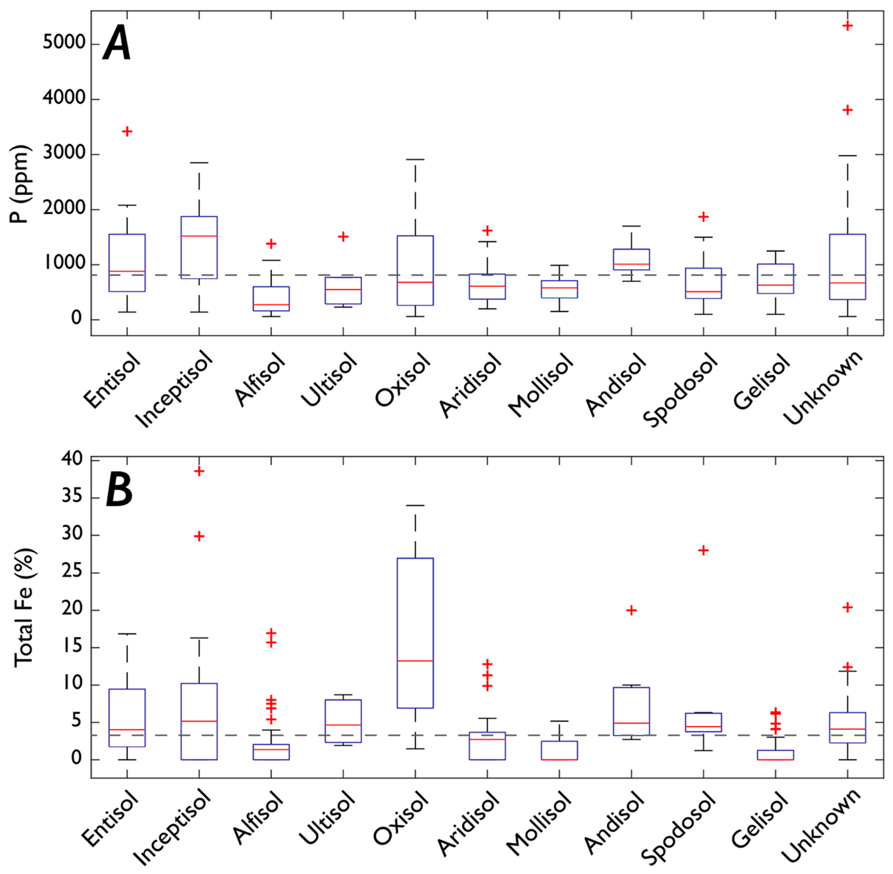
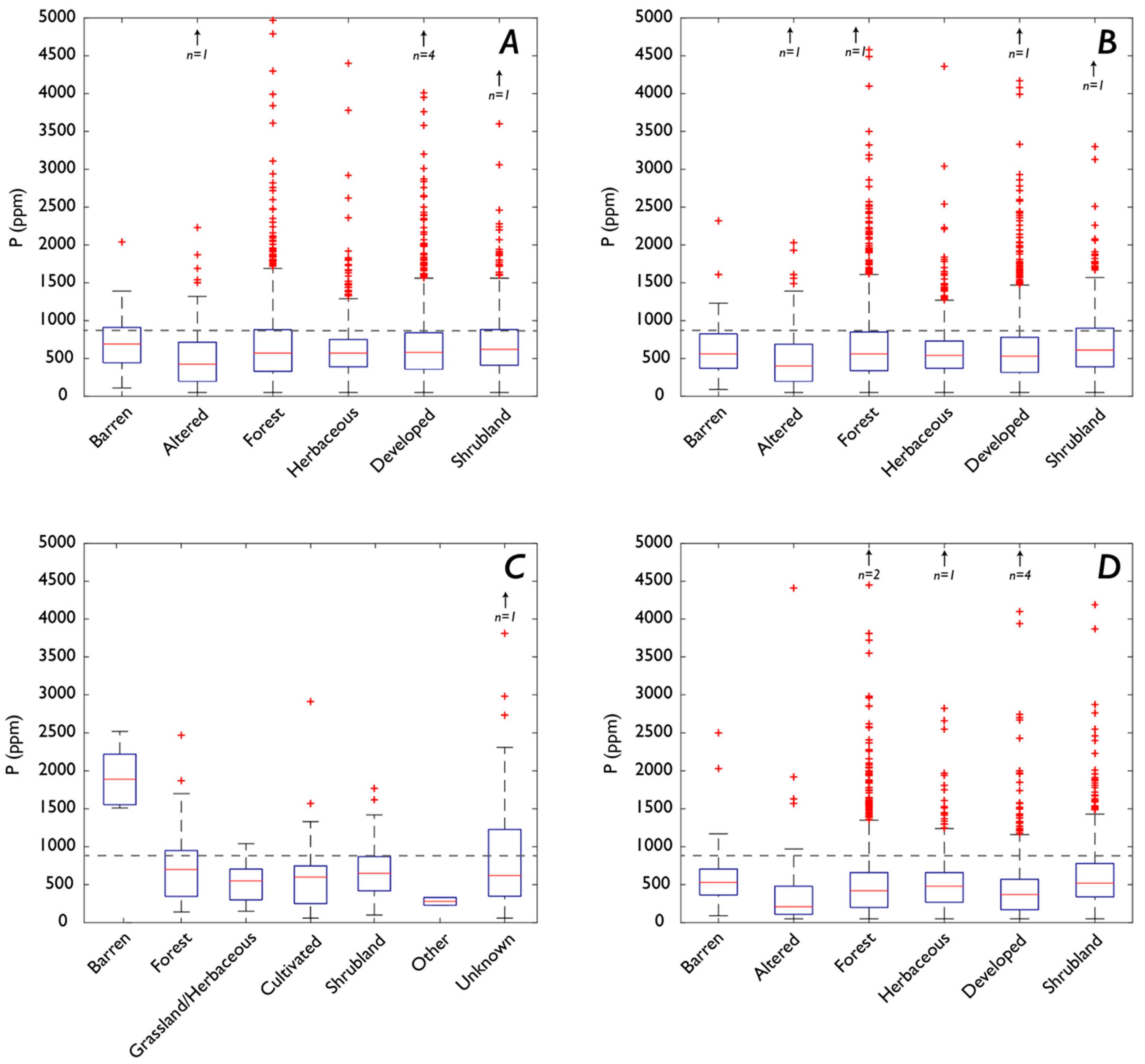
3.1. Fe and P: Concentrations, Soil Order, and Vegetation
3.1.1. P
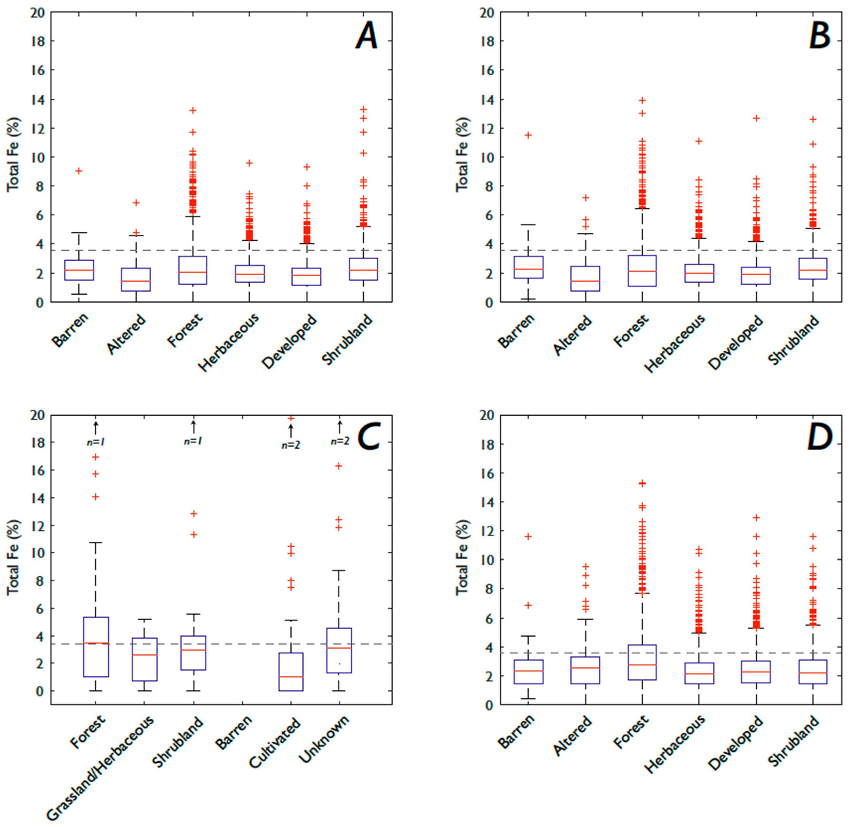
3.1.2. Fe
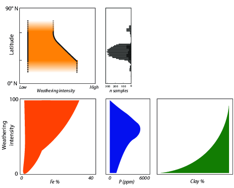
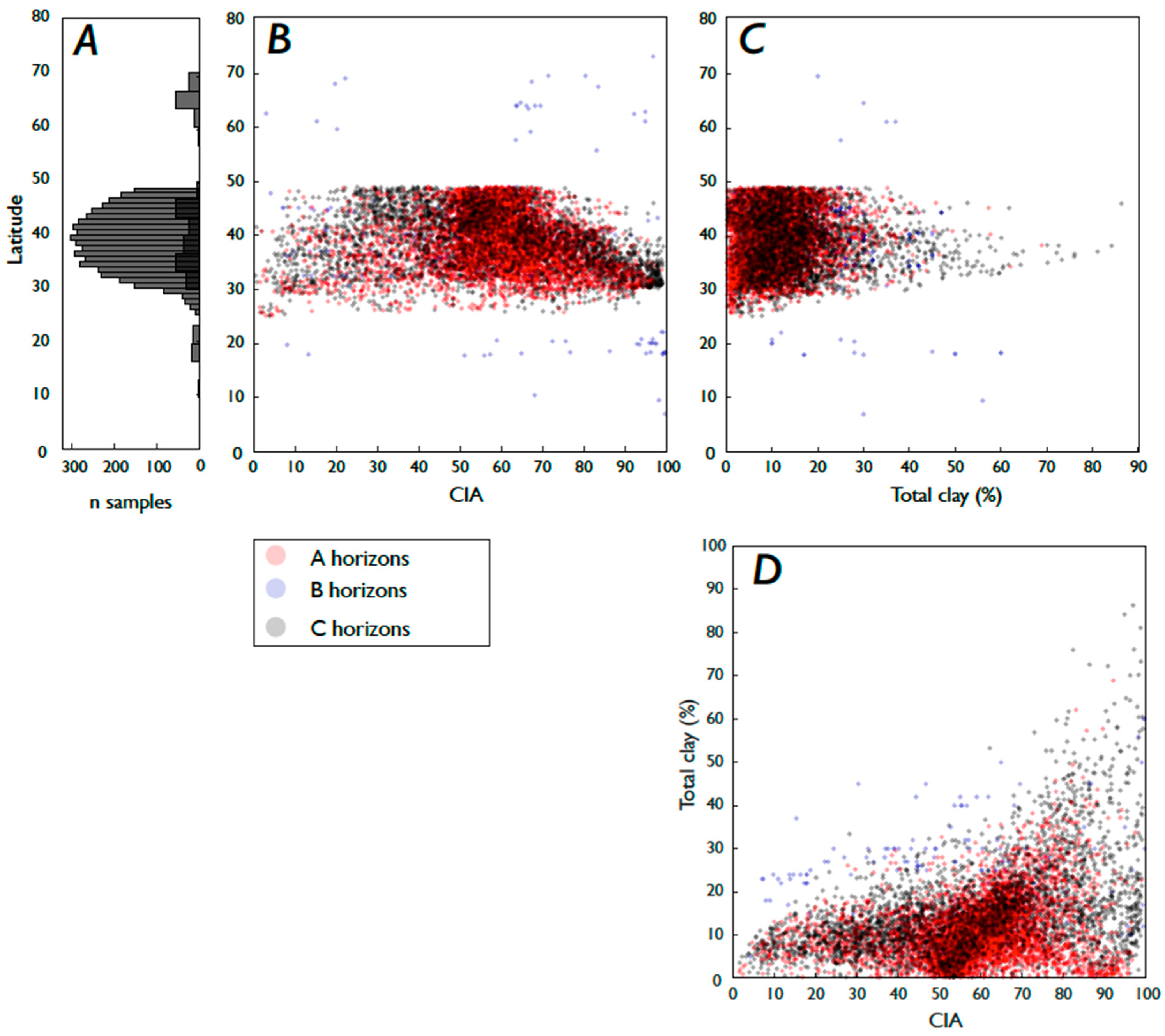
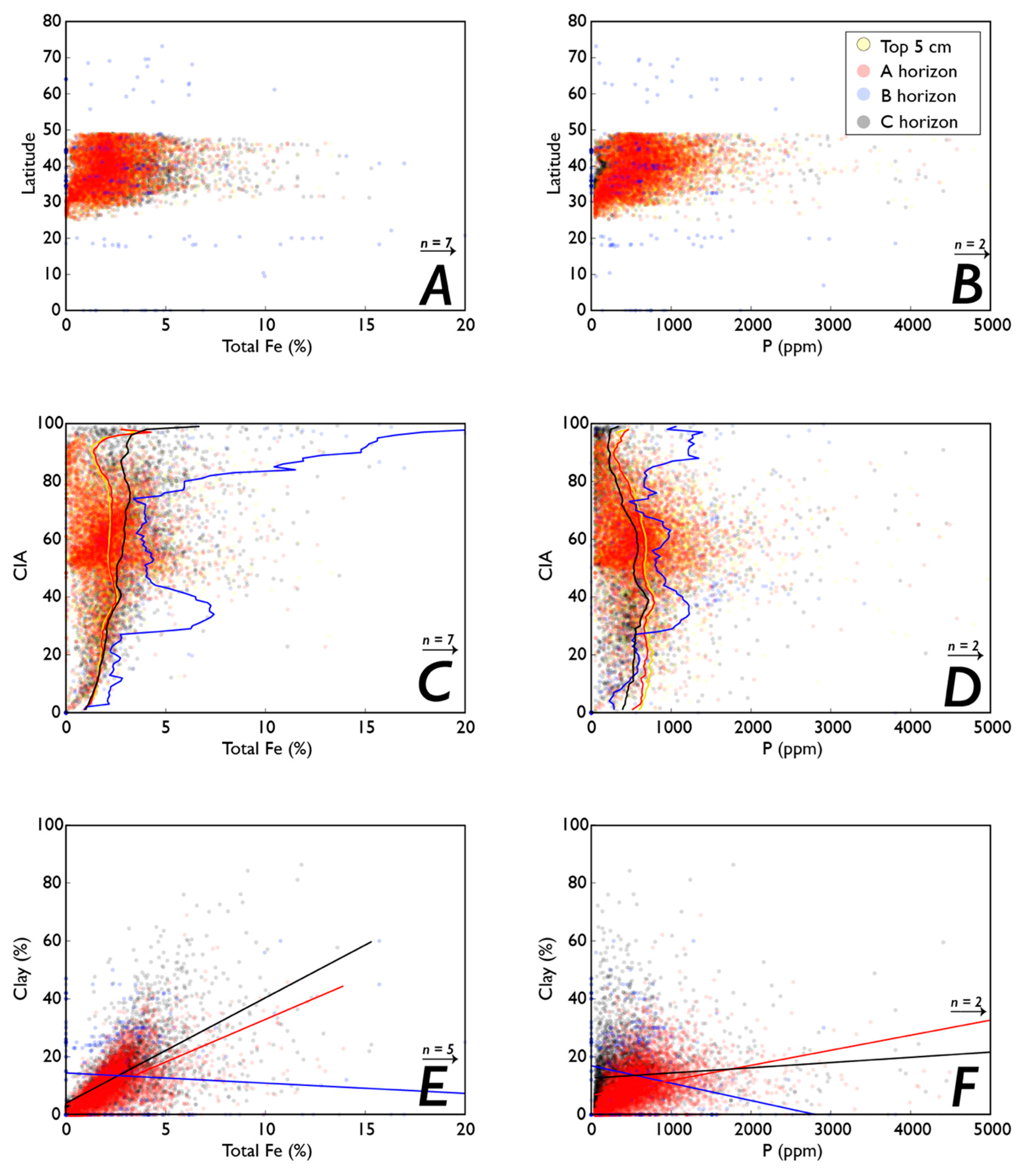
3.2. Fe and P: Latitude, Weathering, Soil Order, and Clay Content
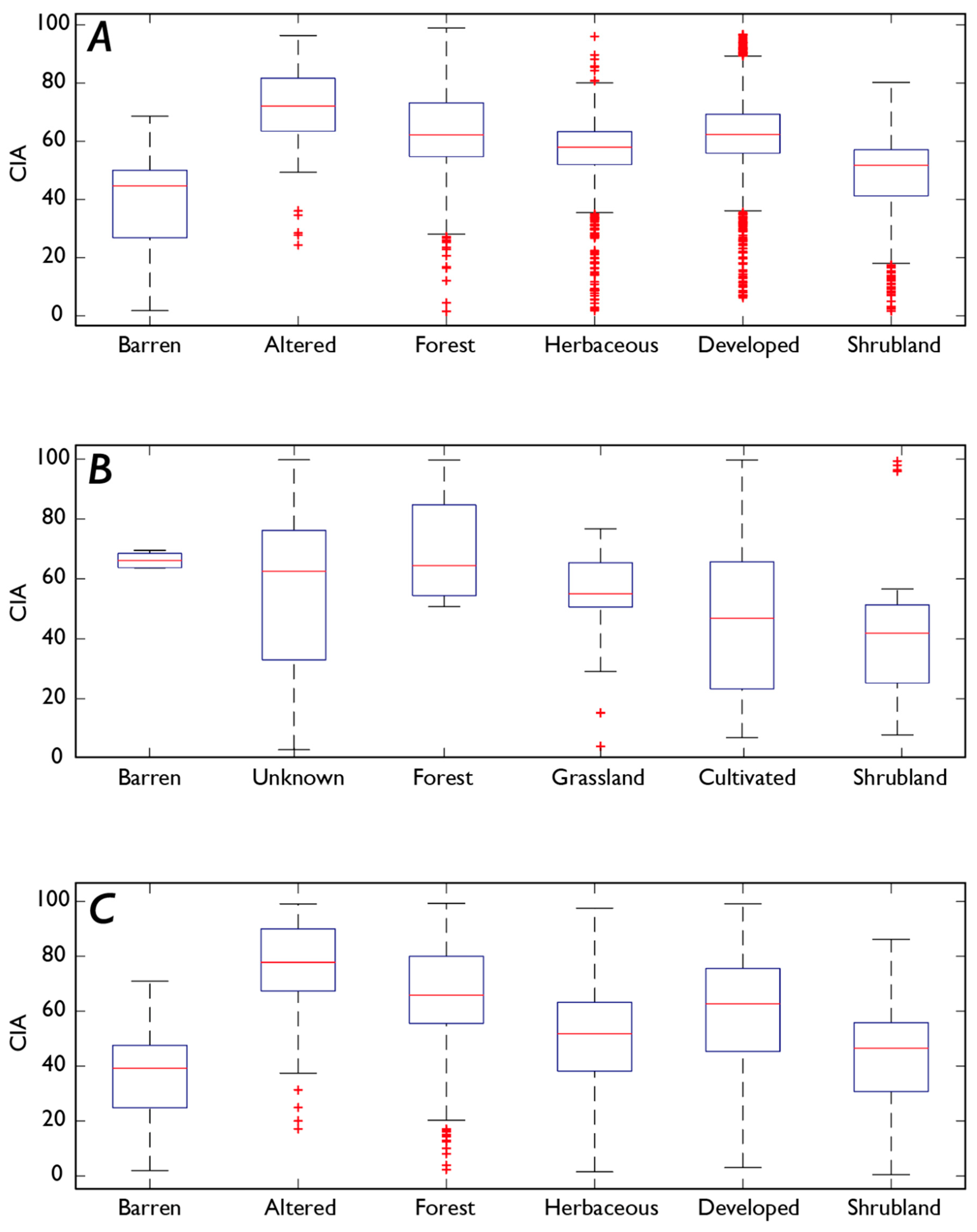
3.3. Weathering, Clay Content, and Vegetation
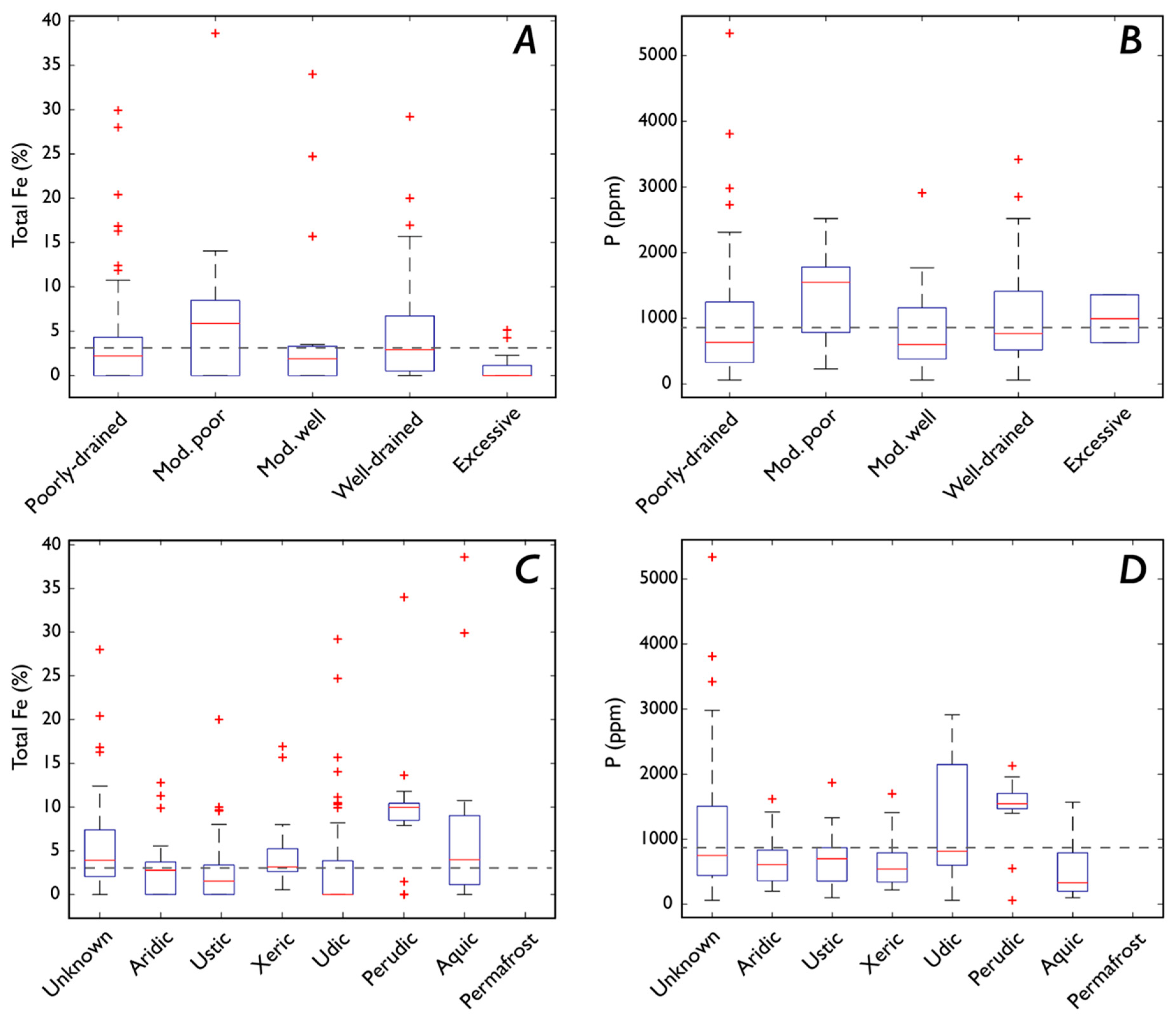
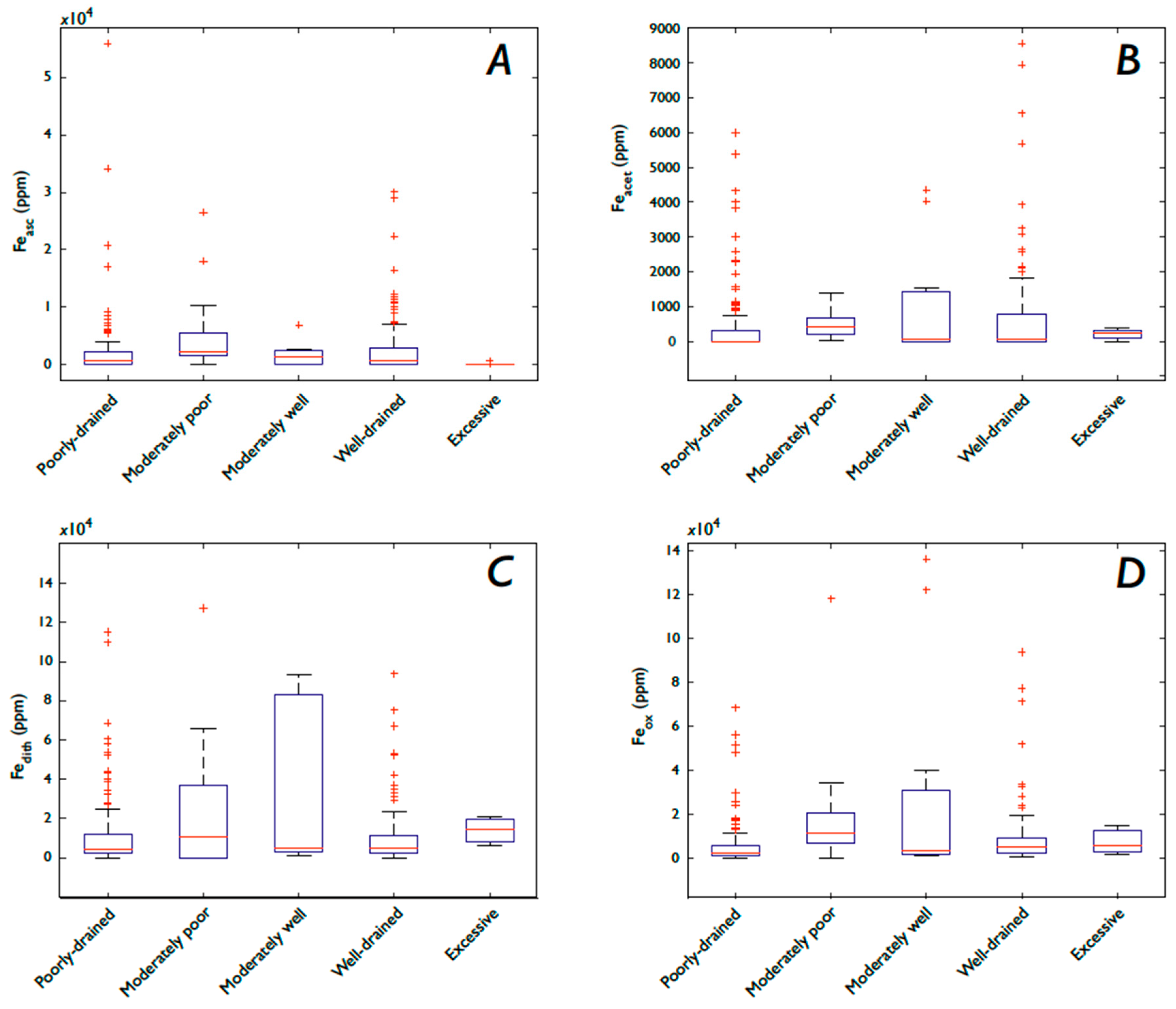
3.4. Fe and P: Drainage and Soil Moisture
3.5. Fe Speciation
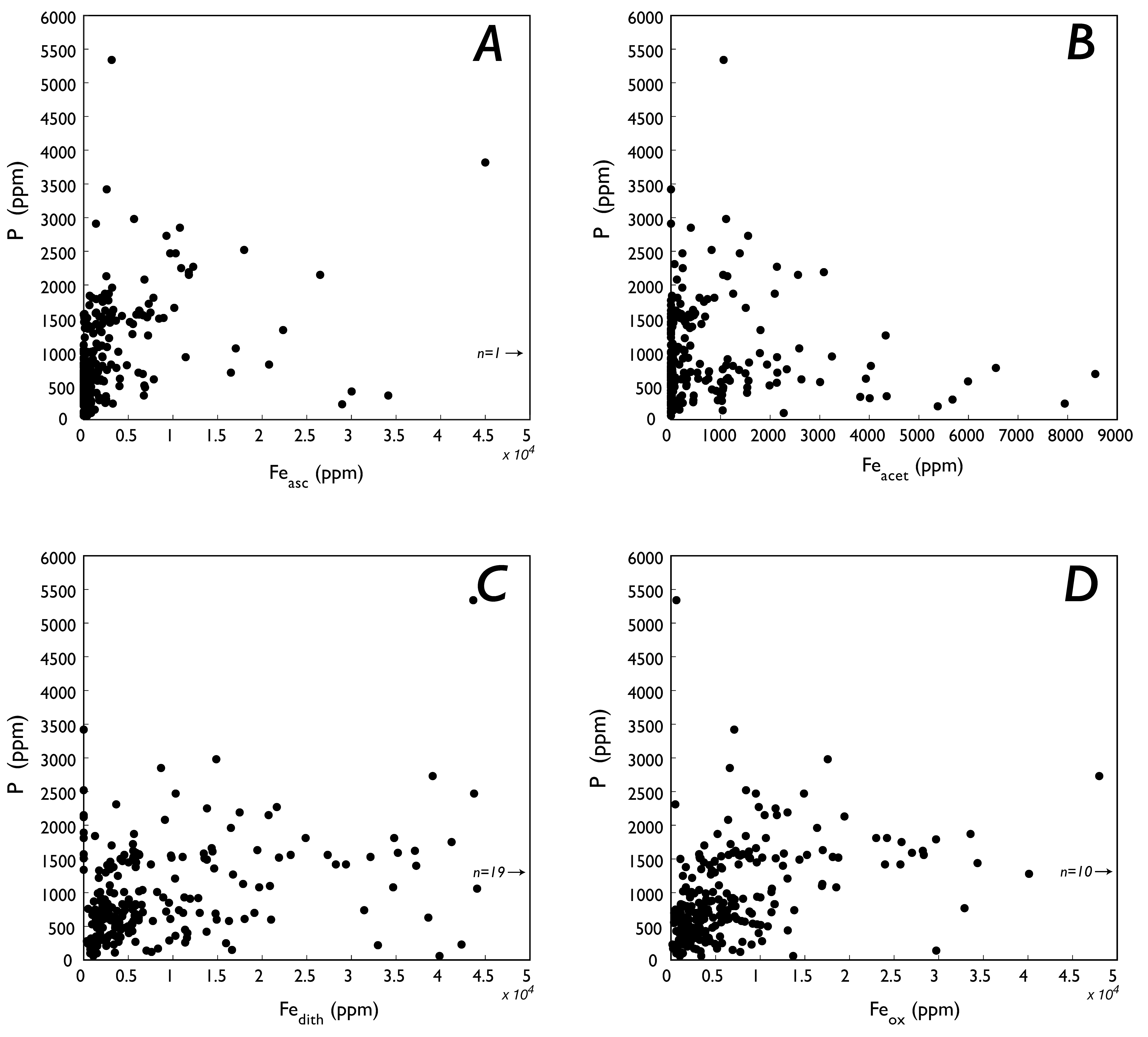
3.5.1. Fe Speciation and P
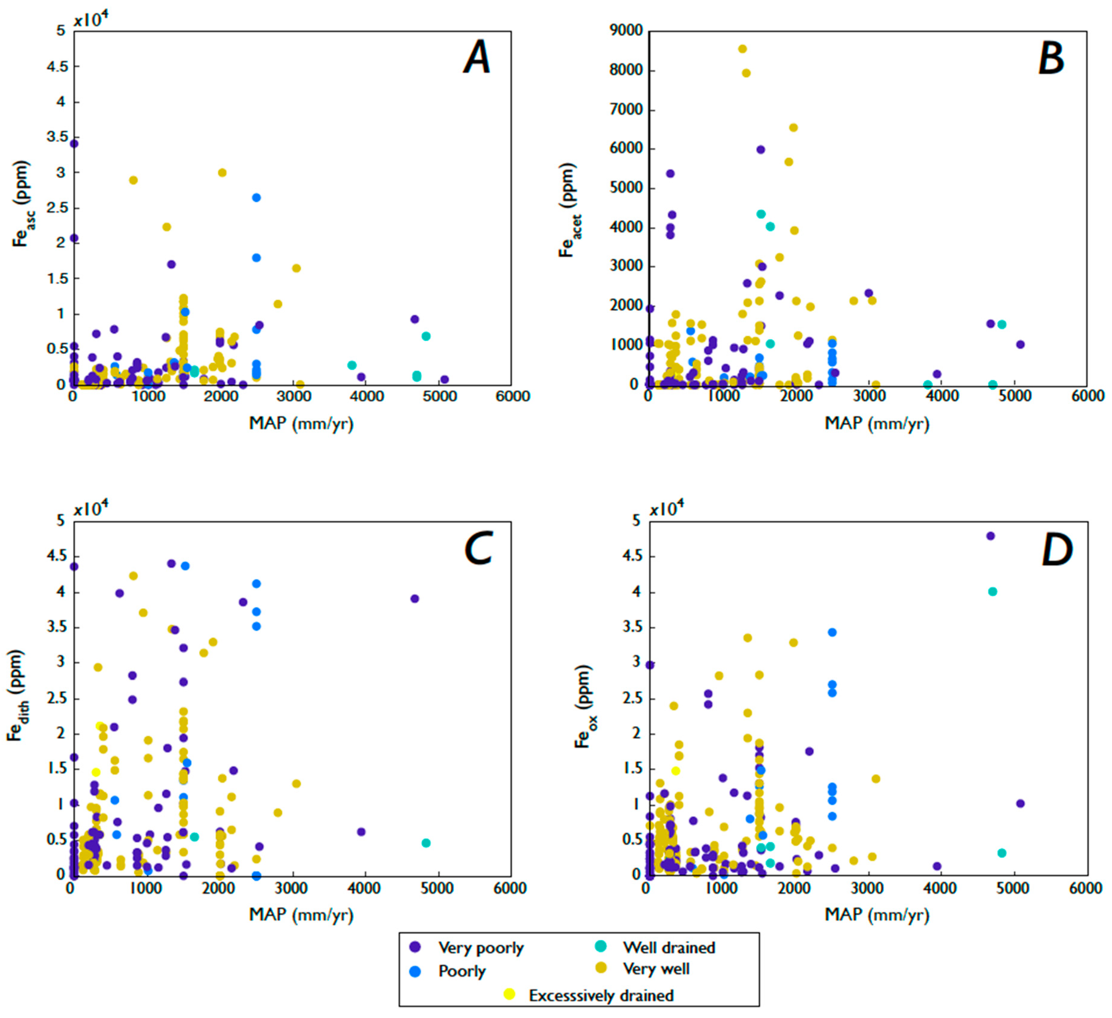
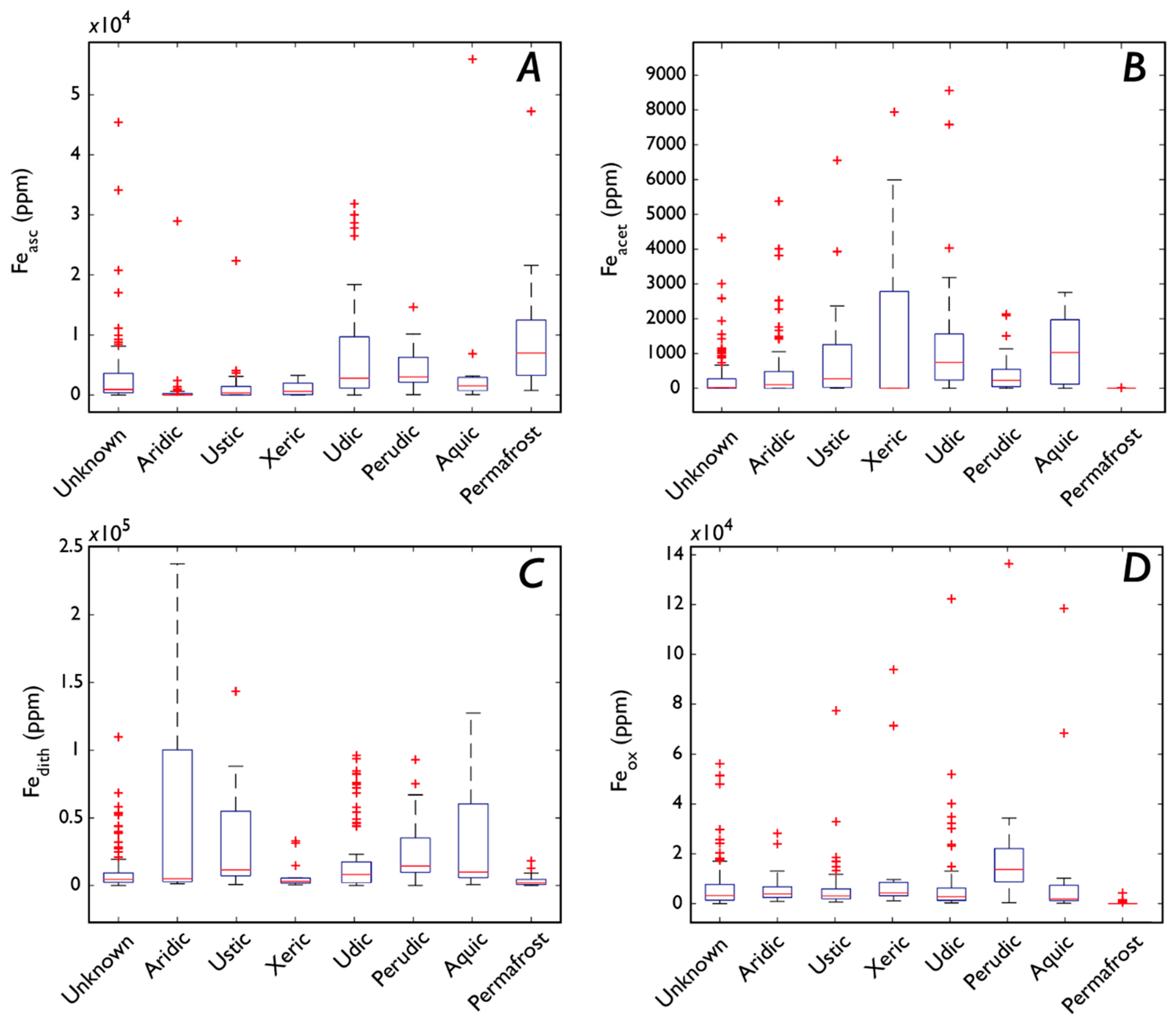
3.5.2. Fe Speciation, Precipitation, Soil Moisture, and Drainage
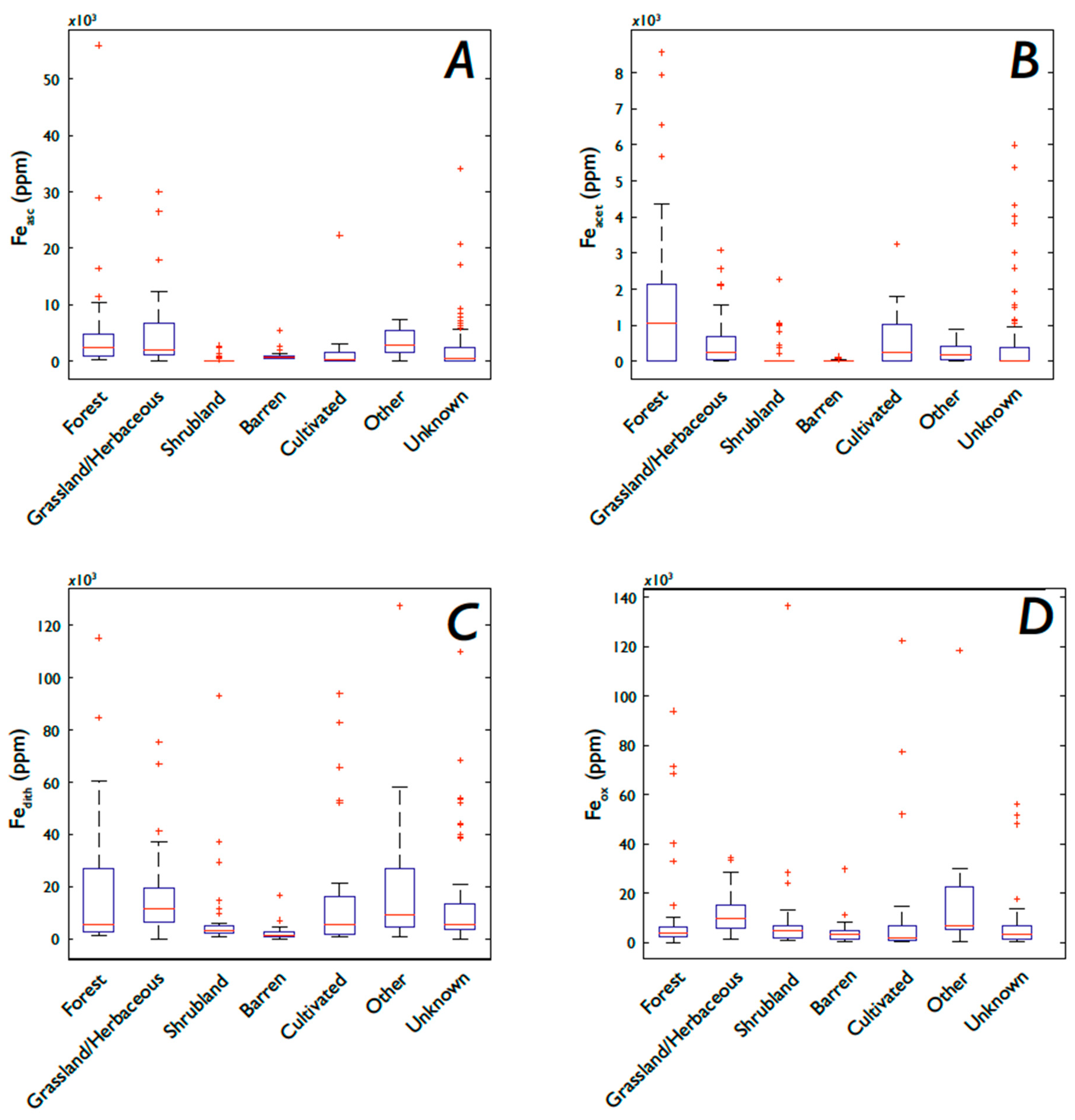
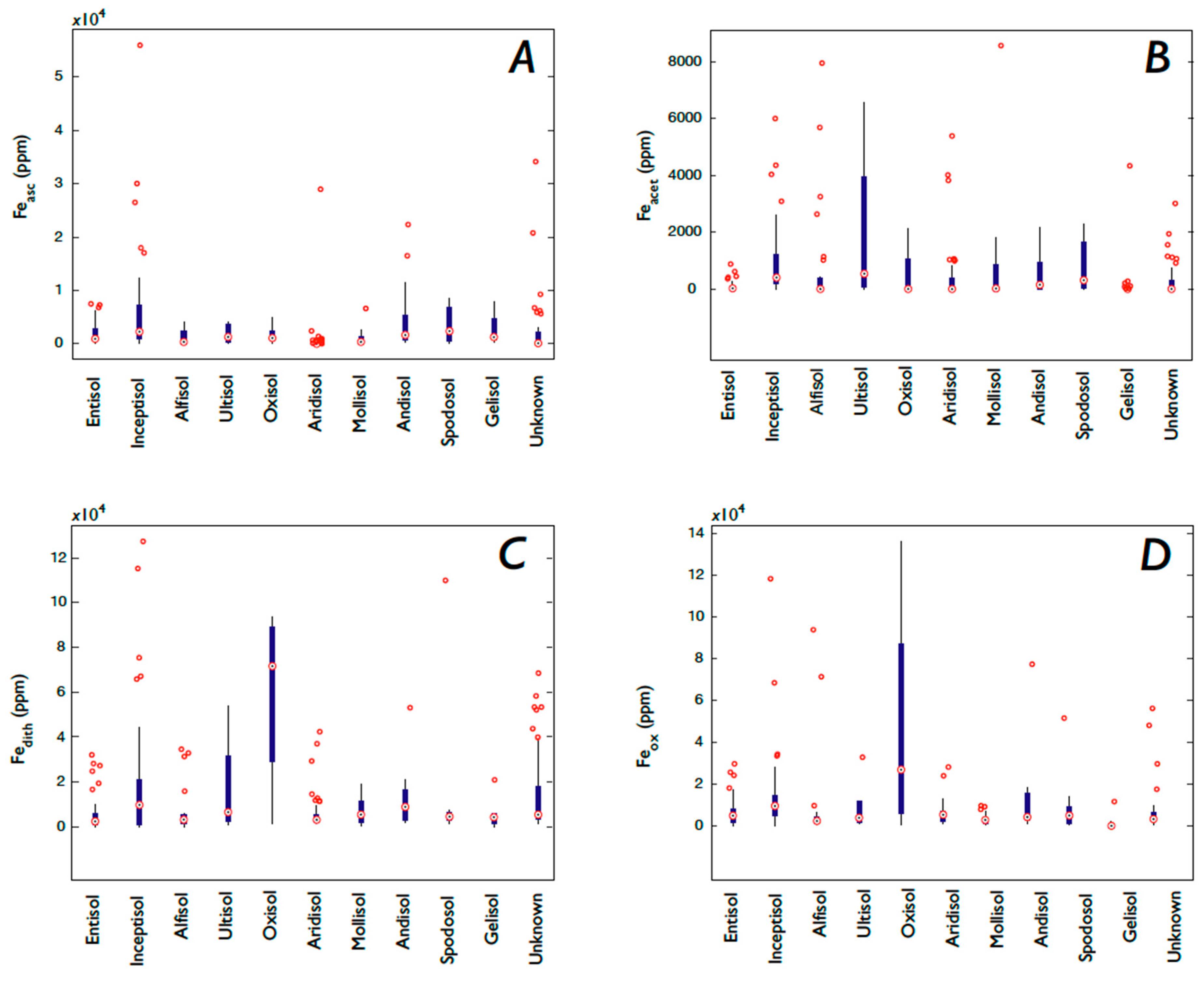
3.5.3. Fe Speciation, Vegetation, and Soil Order
3.6. Organic Carbon
3.7. Parent Material
3.8. Principle Components Analysis
4. Discussion
4.1. How do Latitude, Weathering, and Clay Content Associate with P and Fe Concentrations?
4.2. How Do Precipitation, Soil Moisture, and Soil Drainage Affect P and Fe Concentrations, and Fe Species?
4.2.1. How Does Soil Redox Affect P?
4.2.2. How Does Soil Redox Affect Fe Concentrations and Speciation?
4.3. How Do Fe Species Associate with P?
4.4. How Does Vegetation Affect P and Fe Concentrations?
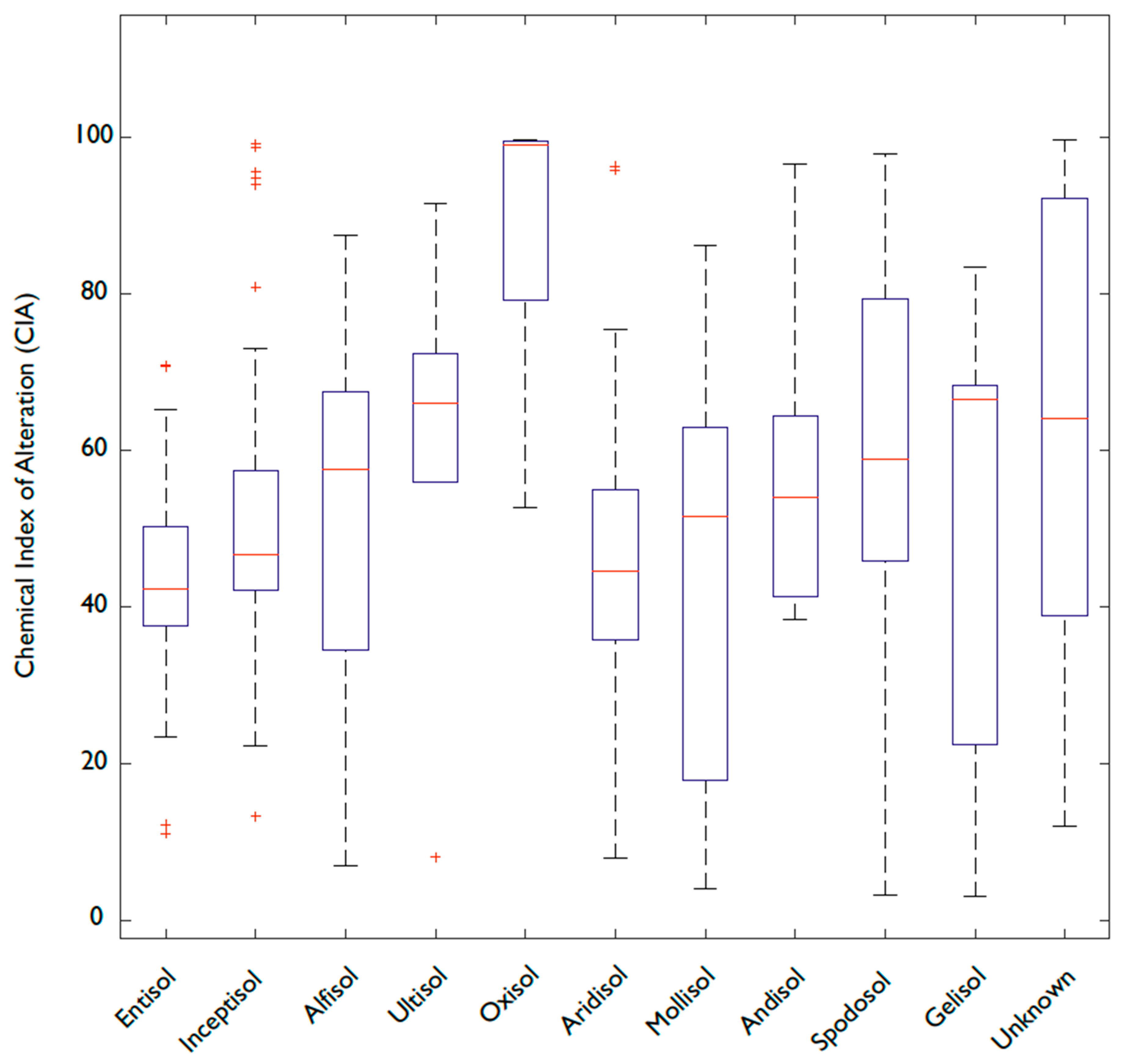
4.5. Is Soil Order Predictive of P and Fe Concentrations?
4.6. Implications for P in Modern Soils, Climate Change, and Soil Fertility/Food Security
4.6.1. Soil P, Erosion and Transport, and Human Activity
4.6.2. Weathering, Climate Change, and Soil P
4.6.3. Soil P, Plants, and Agriculture
4.7. Implications for P in the Fossil Record of Soils and Its Geologic Use
4.7.1. Heterogeneity and Paleosol Representativeness
4.7.2. Paleosol Fe, Atmospheric Oxygen Reconstructions, and Microbial Life
4.7.3. Continental Weathering, Nutrient Fluxes, and the Atmosphere
4.7.4. Vegetation and P in the Phanerozoic (542 Ma Onwards)
5. Conclusions
Supplementary Materials
Author Contributions
Funding
Acknowledgments
Conflicts of Interest
References
- Froelich, P.N.; Bender, M.L.; Luedtke, N.A.; Heath, G.R.; Devries, T. The marine phosphorus cycle. Am. J. Sci. 1982, 282, 474–511. [Google Scholar] [CrossRef]
- Du, E.; Terrer, C.; Pellegrini, A.F.A.; Ahlström, A.; Van Lissa, C.J.; Zhao, X.; Xia, N.; Wu, X.; Jackson, R.B. Global patterns of terrestrial nitrogen and phosphorus limitation. Nat. Geosci. 2020, 13, 221–226. [Google Scholar] [CrossRef]
- Correll, D.L. The Role of Phosphorus in the Eutrophication of Receiving Waters: A Review. J. Environ. Qual. 1998, 27, 261–266. [Google Scholar] [CrossRef] [Green Version]
- Filippelli, G.M. The Global Phosphorus Cycle. Rev. Miner. Geochem. 2002, 48, 391–425. [Google Scholar] [CrossRef] [Green Version]
- Filippelli, G.M. The Global Phosphorus Cycle: Past, Present, and Future. Elements 2008, 4, 89–95. [Google Scholar] [CrossRef]
- Peretyazhko, T.; Sposito, G. Iron(III) reduction and phosphorus solubilzation in humid tropical soils. Geochim. Cosmochim. Acta 2005, 69, 3643–3652. [Google Scholar] [CrossRef]
- Chacon, N.; Silver, W.L.; Dubinsky, E.A.; Cusack, D.F. Iron Reduction and Soil Phosphorus Solubilization in Humid Tropical Forests Soils: The Roles of Labile Carbon Pools and an Electron Shuttle Compound. Biogeochemistry 2006, 78, 67–84. [Google Scholar] [CrossRef]
- Fink, J.R.; Inda, A.V.; Tiecher, T.; Barrón, V. Iron oxides and organic matter on soil phosphorus availability. Ciência Agrotec. 2016, 40, 369–379. [Google Scholar] [CrossRef] [Green Version]
- Herndon, E.M.; Kinsman-Costello, L.; Duroe, K.A.; Mills, J.; Kane, E.S.; Sebestyen, S.D.; Thompson, A.A.; Wullschleger, S.D. Iron (oxyhydr) oxides serve as phosphate traps in tundra and boreal peat soils. J. Geophys. Res. Biogeosci. 2019, 124, 227–246. [Google Scholar] [CrossRef]
- Reinhard, C.T.; Planavsky, N.J.; Gill, B.C.; Ozaki, K.; Robbins, L.J.; Lyons, T.W.; Fischer, W.W.; Wang, C.; Cole, N.J.P.D.B.; Konhauser, L.J.R.K.O. Evolution of the global phosphorus cycle. Nat. Cell Biol. 2017, 541, 386–389. [Google Scholar] [CrossRef]
- Lenton, T.M.; Daines, S.J.; Mills, B.J. COPSE reloaded: An improved model of biogeochemical cycling over Phanerozoic time. Earth Sci. Rev. 2018, 178, 1–28. [Google Scholar] [CrossRef]
- Guidry, M.W.; Mackenzie, F.T. Apatite weathering and the Phanerozoic phosphorus cycle. Geology 2000, 28, 631–634. [Google Scholar] [CrossRef]
- D’Antonio, M.P.; Ibarra, D.E.; Boyce, C.K. Land plant evolution decreased, rather than increased, weathering rates. Geology 2019, 48, 29–33. [Google Scholar] [CrossRef]
- Jenny, H.J. Factors in Soil Formation; McGraw-Hill: New York, NY, USA, 1941. [Google Scholar]
- Quirk, J.; Leake, J.R.; Johnson, D.A.; Taylor, L.L.; Saccone, L.; Beerling, D.J. Constraining the role of early land plants in Palaeozoic weathering and global cooling. Proc. R. Soc. B Boil. Sci. 2015, 282, 20151115. [Google Scholar] [CrossRef] [Green Version]
- Leake, J.R.; Read, D.J. Mycorrhizal symbioses and pedogenesis throughout Earth’s history. In Mycorrhizal Mediation of Soil: Fertility, Structure, and Carbon Storage; Johnson, N.C., Gehring, C., Jansa, J., Eds.; Elsevier: New York, NY, USA, 2017; pp. 9–33. [Google Scholar]
- Chadwick, O.; Derry, L.; Vitousek, P.M.; Huebert, B.J.; Hedin, L. Changing sources of nutrients during four million years of ecosystem development. Nat. Cell Biol. 1999, 397, 491–497. [Google Scholar] [CrossRef]
- Okin, G.S.; Mahowald, N.; Chadwick, O.A.; Artaxo, P. Impact of desert dust on the biogeochemistry of phosphorus in terrestrial ecosystems. Glob. Biogeochem. Cycles 2004, 18, 2005. [Google Scholar] [CrossRef] [Green Version]
- Walker, T.; Syers, J. The fate of phosphorus during pedogenesis. Geoderma 1976, 15, 1–19. [Google Scholar] [CrossRef]
- Wardle, D.A.; Walker, L.R.; Bardgett, R.D. Ecosystem Properties and Forest Decline in Contrasting Long-Term Chronosequences. Science 2004, 305, 509–513. [Google Scholar] [CrossRef] [Green Version]
- Arvin, L.J.; Riebe, C.S.; Aciego, S.; Blakowski, M.A. Global patterns of dust and bedrock nutrient supply to montane ecosystems. Sci. Adv. 2017, 3, eaao1588. [Google Scholar] [CrossRef] [Green Version]
- Gu, C.; Hart, S.C.; Turner, B.L.; Hu, Y.; Meng, Y.; Zhu, M. Aeolian dust deposition and the perturbation of phosphorus transformations during long-term ecosystem development in a cool, semi-arid environment. Geochim. Cosmochim. Acta 2019, 246, 498–514. [Google Scholar] [CrossRef]
- Sherman, G.D. The genesis and morphology of the alumina-rich laterite clays. In Problems of Clay and Laterite Genesis; Fredericksen, A.F., Ed.; American Institute of Mining and Metallurgical Engineering: New York, NY, USA, 1952; pp. 154–161. [Google Scholar]
- Jobbágy, E.G.; Jackson, R.B. The distribution of soil nutrients with depth: Global patterns and the imprint of plants. Biogeochemistry 2001, 53, 51–77. [Google Scholar] [CrossRef]
- Riebe, C.S.; Kirchner, J.W.; Finkel, R.C. Erosional and climatic effects on long-term chemical weathering rates in granitic landscapes spanning diverse climate regimes. Earth Planet. Sci. Lett. 2004, 224, 547–562. [Google Scholar] [CrossRef]
- Dixon, J.L.; Heimsath, A.M.; Amundson, R. The critical role of climate and saprolite weathering in landscape evolution. Earth Surf. Process. Landf. 2009, 34, 1507–1521. [Google Scholar] [CrossRef]
- Gabet, E.J.; Mudd, S.M. A theoretical model coupling chemical weathering rates with denudation rates. Geology 2009, 37, 151–154. [Google Scholar] [CrossRef]
- Dixon, J.L.; Hartshorn, A.S.; Heimsath, A.M.; DiBiase, R.A.; Whipple, K.X. Chemical weathering response to tectonic forcing: A soils perspective from the San Gabriel Mountains, California. Earth Planet. Sci. Lett. 2012, 40–49. [Google Scholar] [CrossRef]
- Hewawasam, T.; Von Blanckenburg, F.; Bouchez, J.; Dixon, J.L.; Schuessler, J.A.; Maekeler, R. Slow advance of the weathering front during deep, supply-limited saprolite formation in the tropical Highlands of Sri Lanka. Geochim. Cosmochim. Acta 2013, 118, 202–230. [Google Scholar] [CrossRef] [Green Version]
- Uhlig, D.; Schuessler, J.A.; Bouchez, J.; Dixon, J.L.; Von Blanckenburg, F. Quantifying nutrient uptake as driver of rock weathering in forest ecosystems by magnesium stable isotopes. Biogeosciences 2017, 14, 3111–3128. [Google Scholar] [CrossRef] [Green Version]
- Eger, A.; Yoo, K.; Almond, P.C.; Boitt, G.; Larsen, I.J.; Condron, L.M.; Wang, X.; Mudd, S.M. Does soil erosion rejuvenate the soil phosphorus inventory? Geoderma 2018, 332, 45–59. [Google Scholar] [CrossRef] [Green Version]
- Kurtz, A.C.; Derry, L.A.; Chadwick, O.A. Accretion of Asian dust to Hawaii soils: Isotopic, elemental, and mineral mass balances. Geochim. Cosmochim. Acta 2001, 65, 1971–1983. [Google Scholar] [CrossRef]
- Porder, S.; Hilley, G.E.; Chadwick, O.A. Chemical weathering, mass loss, and dust inputs across a climate by time matrix in the Hawaiian Islands. Earth Planet. Sci. Lett. 2007, 258, 414–427. [Google Scholar] [CrossRef]
- Swap, R.; Garstang, M.; Greco, S.; Talbot, R.; Kållberg, P. Saharan dust in the Amazon Basin. Tellus B 1992, 44, 133–149. [Google Scholar] [CrossRef] [Green Version]
- Bristow, C.S.; Hudson-Edwards, K.A.; Chappell, A. Fertilizing the Amazon and equatorial Atlantic with West African dust. Geophys. Res. Lett. 2010, 37, 14807. [Google Scholar] [CrossRef]
- Yu, H.; Chin, M.; Yuan, T.; Bian, H.; Remer, L.A.; Prospero, J.M.; Omar, A.; Winker, D.M.; Yang, Y.; Zhang, Y.; et al. The fertilizing role of African dust in the Amazon rainforest: A first multiyear assessment based on data from Cloud-Aerosol Lidar and Infrared Pathfinder Satellite Observations. Geophys. Res. Lett. 2015, 42, 1984–1991. [Google Scholar] [CrossRef]
- Bullard, J.E.; White, K. Dust production and the release of iron oxides resulting from the aeolian abrasion of natural dune sands. Earth Surf. Process. Landforms 2005, 30, 95–106. [Google Scholar] [CrossRef]
- Lafon, S.; Rajot, J.L.; Alfaro, S.C.; Gaudichet, A. Quantification of iron oxides in desert aerosol. Atmos. Environ. 2004, 38, 1211–1218. [Google Scholar] [CrossRef]
- Froelich, P.N. Kinetic control of dissolved phosphate in natural rivers and estuaries: A primer on the phosphate buffer mechanism. Limnol. Oceanogr. 1988, 33, 649–668. [Google Scholar] [CrossRef]
- Karathanasis, A.D. Phosphate Mineralogy and Equilibria in Two Kentucky Alfisols Derived from Ordovician Limestones. Soil Sci. Soc. Am. J. 1991, 55, 1774–1782. [Google Scholar] [CrossRef]
- Turner, B.L.; Cade-Menun, B.J.; Westermann, D.T. Organic Phosphorus Composition and Potential Bioavailability in Semi-Arid Arable Soils of the Western United States. Soil Sci. Soc. Am. J. 2003, 67, 1168–1179. [Google Scholar] [CrossRef] [Green Version]
- Herndon, E.; Albashaireh, A.; Singer, D.; Chowdhury, T.R.; Gu, B.; Graham, D. Influence of iron redox cycling on organo-mineral associations in Arctic tundra soil. Geochim. Cosmochim. Acta 2017, 207, 210–231. [Google Scholar] [CrossRef] [Green Version]
- Kuo, S.; Mikkelsen, D.S. Distribution of Iron and Phosphorus in Flooded and Unflooded Soil Profiles and Their Relation to Phosphorus Adsorption. Soil Sci. 1979, 127, 18–25. [Google Scholar] [CrossRef]
- Peña, F.; Torrent, J. Relationships between phosphate sorption and iron oxides in Alfisols from a river terrace sequence of Mediterranean Spain. Geoderma 1984, 33, 283–296. [Google Scholar] [CrossRef]
- Torrent, J. Fast and Slow Phosphate Sorption by Goethite-Rich Natural Materials. Clays Clay Miner. 1992, 40, 14–21. [Google Scholar] [CrossRef]
- Jaisi, D.; Kukkadapu, R.K.; Stout, L.M.; Varga, T.; Blake, R.E. Biotic and Abiotic Pathways of Phosphorus Cycling in Minerals and Sediments: Insights from Oxygen Isotope Ratios in Phosphate. Environ. Sci. Technol. 2011, 45, 6254–6261. [Google Scholar] [CrossRef] [PubMed]
- Prietzel, J.; Klysubun, W.; Werner, F. Speciation of phosphorus in temperate zone forest soils as assessed by combined wet-chemical fractionation and XANES spectroscopy. J. Plant Nutr. Soil Sci. 2016, 179, 168–185. [Google Scholar] [CrossRef]
- Coronato, F.R.; Bertiller, M.B. Climatic controls of soil moisture dynamics in an arid steppe of northern Patagonia, Argentina. Arid. Soil Res. Rehabil. 1997, 11, 277–288. [Google Scholar] [CrossRef]
- Sandvig, R.M.; Phillips, F.M. Ecohydrological controls on soil moisture fluxes in arid to semiarid vadose zones. Water Resour. Res. 2006, 42, W08422. [Google Scholar] [CrossRef]
- Vivoni, E.R.; Rinehard, A.J.; Mendez-Barroso, L.A.; Aragon, C.A.; Bisht, G.; Bayani Cardenas, M.; Engle, E.; Forman, B.A.; Frisbee, M.D.; Gutierrez-Jurado, H.A.; et al. Wyckoff, Vegetation controls on soil moisture distribution in the Valles Caldera, New Mexico, during the North American Monsoon. Ecohydrology 2008, 1, 225–238. [Google Scholar] [CrossRef]
- Gaur, N.; Mohanty, B.P. Evolution of physical controls for soil moisture in humid and subhumid watersheds. Water Resour. Res. 2013, 49, 1244–1258. [Google Scholar] [CrossRef]
- Fatichi, S.; Katul, G.G.; Ivanov, V.Y.; Pappas, C.; Paschalis, A.; Consolo, A.; Kim, J.; Burlando, P. Abiotic and biotic controls of soil moisture spatiotemporal variability and the occurrence of hysteresis. Water Resour. Res. 2015, 51, 3505–3524. [Google Scholar] [CrossRef]
- Wang, T.; Wedin, D.; Franz, T.E.; Hiller, J. Effect of vegetation on the temporal stability of soil moisture in grass-stabilized semi-arid sand dunes. J. Hydrol. 2015, 521, 447–459. [Google Scholar] [CrossRef]
- Surridge, B.W.J.; Heathwaite, A.L.; Baird, A.J. The Release of Phosphorus to Porewater and Surface Water from River Riparian Sediments. J. Environ. Qual. 2007, 36, 1534–1544. [Google Scholar] [CrossRef] [PubMed]
- KerrMichele, J.G.; Burford, M.A.; Olley, J.; Udy, J.W. Phosphorus sorption in soils and sediments: Implications for phosphate supply to a subtropical river in southeast Queensland, Australia. Biogeochemistry 2011, 102, 73–85. [Google Scholar] [CrossRef]
- Berner, R.A. The carbon cycle and carbon dioxide over Phanerozoic time: The role of land plants. Philos. Trans. R. Soc. B Biol. Sci. 1998, 353, 75–82. [Google Scholar] [CrossRef] [Green Version]
- Martin, J.H.; Fitzwater, S.E. Iron deficiency limits phytoplankton growth in the north-east Pacific subarctic. Nat. Cell Biol. 1988, 331, 341–343. [Google Scholar] [CrossRef]
- Martin, J.H.; Coale, K.H.; Johnson, K.S.; Fitzwater, S.E.; Gordon, R.M.; Tanner, S.J.; Hunter, C.N.; Elrod, V.A.; Nowicki, J.L.; Coley, T.L.; et al. Testing the iron hypothesis in ecosystems of the equatorial Pacific Ocean. Nature 1994, 371, 123–129. [Google Scholar] [CrossRef]
- Coale, K.H. Effects of iron, manganese, copper, and zinc enrichments on productivity and biomass in the subarctic Pacific. Limnol. Oceanogr. 1991, 36, 1851–1864. [Google Scholar] [CrossRef]
- Boyd, P.W.; Watson, A.J.; Law, C.S.; Abraham, E.R.; Trull, T.; Murdoch, R.; Bakker, D.C.E.; Bowie, A.R.; Buesseler, K.O.; Chang, H.; et al. A mesoscale phytoplankton bloom in the polar Southern Ocean stimulated by iron fertilization. Nature 2000, 407, 695–702. [Google Scholar] [CrossRef]
- Berner, R.A.; Rao, J.-L. Phosphorus in sediments of the Amazon River and estuary: Implications for the global flux of phosphorus to the sea. Geochim. Cosmochim. Acta 1994, 58, 2333–2339. [Google Scholar] [CrossRef]
- Moulton, K.L.; Berner, R.A. Quantification of the effect of plants on weathering: Studies in Iceland. Geology 1998, 26, 895. [Google Scholar] [CrossRef]
- Lenton, T.M.; Dahl, T.W.; Daines, S.J.; Mills, B.J.W.; Ozaki, K.; Saltzman, M.R.; Porada, P. Earliest land plants created modern levels of atmospheric oxygen. Proc. Natl. Acad. Sci. USA 2016, 113, 9704–9709. [Google Scholar] [CrossRef] [Green Version]
- Smith, D.B.; Cannon, W.F.; Woodruff, L.G.; Solano, F.; Ellefsen, K.J. Geochemical and Mineralogical Maps for Soils of the Conterminous United States; U.S. Geological Survey Open-File Report; United States Geological Survey: Denver, CO, USA, 2014; 386p, ISSN 2331-1258. [CrossRef]
- Box, E.O. Plant functional types and climate at the global scale. J. Veg. Sci. 1996, 7, 309–320. [Google Scholar] [CrossRef]
- Diaz, S.; Cabido, M. Plant functional types and ecosystem function in relation to global change. J. Veg. Sci. 2009, 8, 463–474. [Google Scholar] [CrossRef]
- DiMichele, W.A.; Montañez, I.P.; Poulsen, C.J.; Tabor, N.J. Climate and vegetational regime shifts in the late Paleozoic ice age earth. Geobiology 2009, 7, 200–226. [Google Scholar] [CrossRef] [PubMed]
- Diefendorf, A.F.; Mueller, K.E.; Wing, S.L.; Koch, P.L.; Freeman, K.H. Global patterns in leaf 13C discrimination and implications for studies of past and future climate. Proc. Natl. Acad. Sci. USA 2010, 107, 5738–5743. [Google Scholar] [CrossRef] [Green Version]
- Poulton, S.W.; Canfield, D.E. Development of a sequential extraction procedure for iron: Implications for iron partitioning in continentally derived particulates. Chem. Geol. 2005, 214, 209–221. [Google Scholar] [CrossRef]
- Raiswell, R.; Vu, H.P.; Brinza, L.; Benning, L.G. The determination of labile Fe in ferrihydrite by ascorbic acid extraction: Methodology, dissolution kinetics and loss of solubility with age and de-watering. Chem. Geol. 2010, 278, 70–79. [Google Scholar] [CrossRef]
- Canfield, D.E.; Raiswell, R.; Westrich, J.T.; Reaves, C.M.; Berner, R.A. The use of chromium reduction in the analysis of reduced inorganic sulfur in sediments and shales. Chem. Geol. 1986, 54, 149–155. [Google Scholar] [CrossRef]
- Sheldon, N.D.; Retallack, G.J. Equation for compaction of paleosols due to burial. Geology 2001, 29, 247–250. [Google Scholar] [CrossRef]
- Raiswell, R.; Hardisty, D.S.; Lyons, T.W.; Canfield, D.E.; Owens, J.D.; Planavsky, N.J.; Poulton, S.W.; Reinhard, C.T. The iron paleoredox proxies: A guide to the pitfalls, problems and proper practice. Am. J. Sci. 2018, 318, 491–526. [Google Scholar] [CrossRef] [Green Version]
- Algeo, T.J.; Liu, J. A re-assessment of elemental proxies for paleoredox analysis. Chem. Geol. 2020, 540, 119549. [Google Scholar] [CrossRef]
- Nesbitt, H.W.; Young, G.M. Early Proterozoic climates and plate motions inferred from major element chemistry of lutites. Nat. Cell Biol. 1982, 299, 715–717. [Google Scholar] [CrossRef]
- Li, C.; Yang, S. Is chemical index of alteration (CIA) a reliable proxy for chemical weathering in global drainage basins? Am. J. Sci. 2010, 310, 111–127. [Google Scholar] [CrossRef]
- Taylor, S.R.; McLennan, S.M. The geochemical evolution of the continental crust. Rev. Geophys. 1995, 33, 241–265. [Google Scholar] [CrossRef]
- Maynard, J.B. Chemistry of Modern Soils as a Guide to Interpreting Precambrian Paleosols. J. Geol. 1992, 100, 279–289. [Google Scholar] [CrossRef]
- Sheldon, N.D.; Tabor, N.J. Quantitative paleoclimatic and paleoenvironmental reconstruction using paleosols. Earth Sci. Rev. 2009, 95, 1–52. [Google Scholar] [CrossRef]
- Gallagher, T.M.; Sheldon, N.D. A new paleothermometer for forest paleosols and its implications for Cenozoic climate. Geology 2013, 41, 647–650. [Google Scholar] [CrossRef]
- Stinchcomb, G.E.; Nordt, L.C.; Driese, S.G.; Lukens, W.E.; Williamson, F.C.; Tubbs, J.D. A data-driven spline model designed to predict paleoclimate using paleosol geochemistry. Am. J. Sci. 2016, 316, 746–777. [Google Scholar] [CrossRef]
- Gérard, F. Clay minerals, iron/aluminum oxides, and their contribution to phosphate sorption in soils—A myth revisited. Geoderma 2016, 262, 213–226. [Google Scholar] [CrossRef]
- Soil Survey Staff. Keys to Soil Taxonomy, 12th ed.; USDA-NRCS: Washington, DC, USA, 2014.
- Maher, B.A. Magnetic properties of modern soils and Quaternary loessic paleosols: Paleoclimatic implications. Palaeogeogr. Palaeoclim. Palaeoecol. 1998, 137, 25–54. [Google Scholar] [CrossRef] [Green Version]
- Maher, B.A.; Possolo, A. Statistical models for use of palaeosol magnetic properties as proxies of palaeorainfall. Glob. Planet. Chang. 2013, 111, 280–287. [Google Scholar] [CrossRef]
- Hyland, E.G.; Badgley, C.; Abrajevitch, A.; Sheldon, N.D.; Van Der Voo, R. A new paleoprecipitation proxy based on soil magnetic properties: Implications for expanding paleoclimate reconstructions. GSA Bull. 2015, 127, B31207.1. [Google Scholar] [CrossRef]
- Maxbauer, D.P.; Feinberg, J.; Fox, D.L. Magnetic mineral assemblages in soils and paleosols as the basis for paleoprecipitation proxies: A review of magnetic methods and challenges. Earth Sci. Rev. 2016, 155, 28–48. [Google Scholar] [CrossRef]
- Prem, M.; Hansen, H.C.B.; Wenzel, W.W.; Heiberg, L.; Sørensen, H.; Borggaard, O.K. High Spatial and Fast Changes of Iron Redox State and Phosphorus Solubility in a Seasonally Flooded Temperate Wetland Soil. Wetlands 2014, 35, 237–246. [Google Scholar] [CrossRef]
- Valaee, M.; Ayoubi, S.; Khormali, F.; Lu, S.G.; Karimzadeh, H.R. Using magnetic susceptibility to discriminate between soil moisture regimes in selected loess and loess-like soils in northern Iran. J. Appl. Geophys. 2016, 127, 23–30. [Google Scholar] [CrossRef]
- Cervi, E.C.; Maher, B.; Poliseli, P.C.; Junior, I.G.D.S.; Da Costa, A.C.S. Magnetic susceptibility as a pedogenic proxy for grouping of geochemical transects in landscapes. J. Appl. Geophys. 2019, 169, 109–117. [Google Scholar] [CrossRef]
- Chaparro, M.A.E.; Moralejo, M.d.P.; Bohnel, H.N.; Acebal, S.G. Iron oxide mineralogy in Mollisols, Aridisols and Entisols from the southwestern Pampean region (Argentina) by environmental magnetism approach. Catena 2020, 190, 104534. [Google Scholar] [CrossRef]
- Hu, P.; Heslop, D.; Rossel, R.A.V.; Roberts, A.P.; Zhao, X. Continental-scale magnetic properties of surficial Australian soils. Earth Sci. Rev. 2020, 203, 103028. [Google Scholar] [CrossRef]
- Borggaard, O.K. The influence of iron oxides on phosphate adsorption by soil. Eur. J. Soil Sci. 1983, 34, 333–341. [Google Scholar] [CrossRef]
- Stone, M.; Mudroch, A. The effect of particle size, chemistry and mineralogy of river sediments on phosphate adsorption. Environ. Technol. Lett. 1989, 10, 501–510. [Google Scholar] [CrossRef]
- Halsted, M.; Lynch, J. Phosphorus responses of C3and C4species. J. Exp. Bot. 1996, 47, 497–505. [Google Scholar] [CrossRef] [Green Version]
- Griffith, D.M.; Cotton, J.M.; Powell, R.L.; Sheldon, N.D.; Still, C.J. Multi-century stasis in C3 and C4 grass distributions across the contiguous United States since the industrial revolution. J. Biogeogr. 2017, 44, 2564–2574. [Google Scholar] [CrossRef]
- Katra, I.; Gross, A.; Swet, N.; Tanner, S.; Krasnov, H.; Angert, A. Substantial dust loss of bioavailable P from agricultural soils. Sci. Rep. 2016, 6, 24736. [Google Scholar] [CrossRef] [PubMed] [Green Version]
- Ewel, B.; Mazzarino, M.J.; Berish, C.W. Tropical Soil Fertility Changes under Monocultures and Successional Communities of Different Structure. Ecol. Appl. 1991, 1, 289–302. [Google Scholar] [CrossRef] [PubMed]
- Gregorich, E.G.; Anderson, D. Effects of cultivation and erosion on soils of four toposequences in the Canadian prairies. Geoderma 1985, 36, 343–354. [Google Scholar] [CrossRef]
- Cotton, J.M.; Jeffery, M.L.; Sheldon, N.D. Climate controls on soil respired CO2 in the United States: Implications for 21st century chemical weathering rates in temperate and arid ecosystems. Chem. Geol. 2013, 358, 37–45. [Google Scholar] [CrossRef]
- Leakey, A.D.B.; Ainsworth, E.A.; Bernacchi, C.J.; Rogers, A.; Long, S.P.; Ort, D.R. Elevated CO2 effects on plant carbon, nitrogen, and water relations: Six important lessons from FACE. J. Exp. Bot. 2009, 60, 2859–2876. [Google Scholar] [CrossRef]
- Terrer, C.; Vicca, S.; Hungate, B.A.; Phillips, R.P.; Prentice, I.C. Mycorrhizal association as a primary control of the CO2 fertilization effect. Science 2016, 353, 72–74. [Google Scholar] [CrossRef] [Green Version]
- Obermeier, W.A.; Lehnert, L.W.; Kammann, C.I.; Müller, C.; Grünhage, L.; Luterbacher, J.; Erbs, M.; Moser, G.; Seibert, R.; Yuan, N.; et al. Reduced CO2 fertilization effect in temperate C3 grasslands under more extreme weather conditions. Nat. Clim. Chang. 2016, 7, 137–141. [Google Scholar] [CrossRef]
- Mearns, L.O.; Gutowski, W.; Jones, R.; Leung, R.; McGinnis, S.; Nunes, A.; Qian, Y. A Regional Climate Change Assessment Program for North America. Eos 2009, 90, 311. [Google Scholar] [CrossRef]
- Bluth, G.J.S.; Kump, L.R. Phanerozoic Paleogeology. Am. J. Sci. 1991, 291, 284–308. [Google Scholar] [CrossRef]
- Crews, T.E.; Kitayama, K.; Fownes, J.H.; Riley, R.H.; Herbert, D.A.; Mueller-Dombois, D.; Vitousek, P.M. Changes in Soil Phosphorus Fractions and Ecosystem Dynamics across a Long Chronosequence in Hawaii. Ecology 1995, 76, 1407–1424. [Google Scholar] [CrossRef]
- Schachtman, D.P.; Reid, R.J.; Ayling, S.M. Phosphorus Uptake by Plants: From Soil to Cell. Plant Physiol. 1998, 116, 447–453. [Google Scholar] [CrossRef] [PubMed] [Green Version]
- Lynch, J.P.; Brown, K.M. Root strategies for phosphorus acquisition. In The Ecophysiology of Plant-Phosphorus Interactions; White, P.J., Hammond, J.P., Eds.; Springer: Dordecht, Germany, 2008. [Google Scholar]
- Smith, S.E.; Jakobsen, I.; Grønlund, M.; Smith, F.A. Roles of Arbuscular Mycorrhizas in Plant Phosphorus Nutrition: Interactions between Pathways of Phosphorus Uptake in Arbuscular Mycorrhizal Roots Have Important Implications for Understanding and Manipulating Plant Phosphorus Acquisition. Plant Physiol. 2011, 156, 1050–1057. [Google Scholar] [CrossRef] [PubMed] [Green Version]
- Fitter, A.H.; Heinemeyer, A.; Husband, R.; Olsen, E.; Ridgway, K.; Staddon, P.L. Global environmental change and the biology of arbuscular mycorrhizas: Gaps and challenges. Can. J. Bot. 2004, 82, 1133–1139. [Google Scholar] [CrossRef]
- Deepika, S.; Kothamasi, D. Soil moisture—A regulator of arbuscular mycorrhizal fungal community assembly and symbiotic phosphorus uptake. Mycorrhiza 2015, 25, 67–75. [Google Scholar] [CrossRef]
- Pearson, J.N.; Jakobsen, I. The relative contribution of hyphae and roots to phosphorus uptake by arbuscular mycorrhizal plants, measured by dual labelling with 32P and 33P. New Phytol. 1993, 124, 489–494. [Google Scholar] [CrossRef]
- Gavito, M.E.; Schweiger, P.; Jakobsen, I. P uptake by arbuscular mycorrhizal hyphae: Effect of soil temperature and atmospheric CO2 enrichment. Glob. Chang. Biol. 2003, 9, 106–116. [Google Scholar] [CrossRef]
- Treseder, K.K. A meta-analysis of mycorrhizal responses to nitrogen, phosphorus, and atmospheric CO2 in field studies. New Phytol. 2004, 164, 347–355. [Google Scholar] [CrossRef] [Green Version]
- Kimball, B.A. Carbon Dioxide and Agricultural Yield: An Assemblage and Analysis of 430 Prior Observations1. Agron. J. 1907, 75, 779–788. [Google Scholar] [CrossRef]
- Solomon, A.M.; Cramer, W. Biospheric implications of global environmental change. In Vegetation Dynamics and Global Change; Solomon, A.M., Shugart, H.H., Eds.; Chapman and Hall: New York, NY, USA, 1993; pp. 25–52. [Google Scholar]
- Caseldine, C. Book Review: Encyclopedia of global environmental change. Volume two—The Earth system: Biological and ecological dimensions of global environmental change. Holocene 2003, 13, 147. [Google Scholar] [CrossRef]
- Girardin, M.P.; Bouriaud, O.; Hogg, E.H.; Kurz, W.; Zimmermann, N.E.; Metsaranta, J.M.; De Jong, R.; Frank, D.C.; Esper, J.; Büntgen, U.; et al. No growth stimulation of Canada’s boreal forest under half-century of combined warming and CO2 fertilization. Proc. Natl. Acad. Sci. USA 2016, 113, E8406–E8414. [Google Scholar] [CrossRef] [PubMed] [Green Version]
- Stein, R.A.; Sheldon, N.D.; Smith, S.Y. Rapid response to anthropogenic climate change by Thuja occidentalis: Implications for past climate reconstructions and future climate predictions. PeerJ 2019, 7, e7378. [Google Scholar] [CrossRef] [PubMed] [Green Version]
- Sheldon, N.D.; Smith, S.Y.; Stein, R.; Ng, M. Carbon isotope ecology of gymnosperms and implications for paleoclimatic and paleoecological studies. Glob. Planet. Chang. 2020, 184, 103060. [Google Scholar] [CrossRef]
- Norby, R.; Warren, J.; Iversen, C.; Garten, C.; Medlyn, B.; McMurtrie, R. CO2 Enhancement of Forest Productivity Constrained by Limited Nitrogen Availability. Nat. Précéd. 2009, 107, 19368–19373. [Google Scholar] [CrossRef]
- Ellsworth, D.S.; Anderson, I.C.; Crous, K.Y.; Cooke, J.; Drake, J.E.; Gherlenda, A.N.; Gimeno, T.E.; Macdonald, C.A.; Medlyn, B.E.; Powell, J.R.; et al. Elevated CO2 does not increase eucalypt forest productivity on a low-phosphorus soil. Nat. Clim. Chang. 2017, 7, 279–282. [Google Scholar] [CrossRef] [Green Version]
- Terrer, C.; Jackson, R.B.; Prentice, I.C.; Keenan, T.; Kaiser, C.; Vicca, S.; Fisher, J.B.; Reich, P.B.; Stocker, B.D.; Hungate, B.; et al. Nitrogen and phosphorus constrain the CO2 fertilization of global plant biomass. Nat. Clim. Chang. 2019, 9, 684–689. [Google Scholar] [CrossRef] [Green Version]
- Cleveland, C.C.; Liptzin, D. C:N:P stoichiometry in soils: Is there a “Redfield ratio” for the microbial biomass? Biogeochemistry 2007, 85, 235–252. [Google Scholar] [CrossRef]
- Maranger, R.; Jones, S.E.; Cotner, J.B. Stoichiometry of carbon, nitrogen, and phosphorus through the freshwater pipe. Limnol. Oceanogr. Lett. 2018, 3, 89–101. [Google Scholar] [CrossRef]
- Berner, R.A. Weathering, plants, and the long-term carbon cycle. Geochim. Cosmochim. Acta 1992, 56, 3225–3231. [Google Scholar] [CrossRef]
- Samreen, S.; Kausar, S. Phosphorus fertilizer: The original and commercial sources. In Phosphorus–Recovery and Recycling; Zhang, T., Ed.; IntechOpen: London, UK, 2019. [Google Scholar] [CrossRef] [Green Version]
- Siebers, N.; Godlinski, F.; Leinweber, P. The phosphorus fertilizer value of bone char for potatoes, wheat, and onions: First results. Agric. For. Res. 2012, 62, 59–64. [Google Scholar]
- Zwetsloot, M.J.; Lehmann, J.; Bauerle, T.; Vanek, S.; Hestrin, R.; Nigussie, A. Phosphorus availability from bone char in a P-fixing soil influenced by root-mycorrhizae-biochar interactions. Plant Soil 2016, 408, 95–105. [Google Scholar] [CrossRef]
- Cordell, D.; Drangert, J.-O.; White, S. The story of phosphorus: Global food security and food for thought. Glob. Environ. Chang. 2009, 19, 292–305. [Google Scholar] [CrossRef]
- Dawson, C.; Hilton, J. Fertiliser availability in a resource-limited world: Production and recycling of nitrogen and phosphorus. Food Policy 2011, 36, S14–S22. [Google Scholar] [CrossRef]
- Cordell, D.; White, S. Sustainable Phosphorus Measures: Strategies and Technologies for Achieving Phosphorus Security. Agronomy 2013, 3, 86–116. [Google Scholar] [CrossRef] [Green Version]
- Retallack, G.J. Soils of the Past: An Introduction to Paleopedology, 2nd ed.; Blackwell Science Ltd.: Oxford, UK, 2001. [Google Scholar]
- Rye, R.; Holland, H.D. Paleosols and the evolution of atmospheric oxygen; a critical review. Am. J. Sci. 1998, 298, 621–672. [Google Scholar] [CrossRef]
- Cerling, T.E. Carbon dioxide in the atmosphere; evidence from Cenozoic and Mesozoic Paleosols. Am. J. Sci. 1991, 291, 377–400. [Google Scholar] [CrossRef]
- Sheldon, N.D. Using paleosols of the Picture Gorge Basalt to reconstruct the Middle Miocene Climatic Optimum. PaleoBios 2006, 26, 27–36. [Google Scholar]
- Driese, S.G.; Jirsa, M.A.; Ren, M.; Brantley, S.L.; Sheldon, N.D.; Parker, D.F.; Schmitz, M.D. Neoarchean paleoweathering of tonalite and metabasalt: Implications for reconstructions of 2.69Ga early terrestrial ecosystems and paleoatmospheric chemistry. Precambrian Res. 2011, 189, 1–17. [Google Scholar] [CrossRef]
- Murakami, T.; Sreenivas, B.; Das Sharma, S.; Sugimori, H. Quantification of atmospheric oxygen levels during the Paleoproterozoic using paleosol compositions and iron oxidation kinetics. Geochim. Cosmochim. Acta 2011, 75, 3982–4004. [Google Scholar] [CrossRef]
- Driese, S.G. Pedogenic Translocation of Fe in Modern and Ancient Vertisols and Implications for Interpretations of the Hekpoort Paleosol (2.25 Ga). J. Geol. 2004, 112, 543–560. [Google Scholar] [CrossRef]
- Retallack, G.J.; Noffke, N.; Chafetz, H. Criteria for Distinguishing Microbial Mats and Earths. Soc. Econ. Paleont. Mineral. Spec. Pap. 2012, 101, 136–152. [Google Scholar]
- Hyland, E.G.; Sheldon, N.D. Examining the spatial consistency of palaesol proxies: Implications for palaeoclimatic and palaeoenvironmental reconstructions in terrestrial sedimentary basins. Sedimentology 2016, 63, 959–971. [Google Scholar] [CrossRef]
- Beukes, N.J.; Dorland, H.; Gutzmer, J.; Nedachi, M.; Ohmoto, H. Tropical laterites, life on land, and the history of atmospheric oxygen in the Paleoproterozoic. Geology 2002, 30, 491. [Google Scholar] [CrossRef]
- Beraldi-Campesi, H.; Hartnett, H.E.; Anbar, A.; Gordon, G.W.; Garcia-Pichel, F. Effect of biological soil crusts on soil elemental concentrations: Implications for biogeochemistry and as traceable biosignatures of ancient life on land. Geobiology 2009, 7, 348–359. [Google Scholar] [CrossRef]
- Donnadieu, Y.; Goddéris, Y.; Ramstein, G.; Nédélec, A.; Meert, J. A ‘snowball Earth’ climate triggered by continental break-up through changes in runoff. Nature 2004, 541, 303–306. [Google Scholar] [CrossRef]
- Mills, B.; Watson, A.J.; Goldblatt, C.; Boyle, R.; Lenton, T.M. Timing of Neoproterozoic glaciations linked to transport-limited global weathering. Nat. Geosci. 2011, 4, 861–864. [Google Scholar] [CrossRef]
- Dzombak, R.M.; Sheldon, N.D. Three billion years of continental weathering and implications for marine biogeochemistry. In Proceedings of the Goldschmidt Annual Geochemical Conference, Honolulu, HI, USA, 21–26 June 2020. Abstract Number 635. [Google Scholar]
- Canfield, D. A new model for Proterozoic ocean chemistry. Nat. Cell Biol. 1998, 396, 450–453. [Google Scholar] [CrossRef]
- Habicht, K.S.; Gade, M.; Thamdrup, B.; Berg, P.; Canfield, D.E. Calibration of Sulfate Levels in the Archean Ocean. Science 2002, 298, 2372–2374. [Google Scholar] [CrossRef] [Green Version]
- Halevy, I.; Peters, S.E.; Fischer, W.W. Sulfate Burial Constraints on the Phanerozoic Sulfur Cycle. Science 2012, 337, 331–334. [Google Scholar] [CrossRef] [Green Version]
- Fakhraee, M.; Hancisse, O.; Canfield, D.E.; Crowe, S.A.; Katsev, S. Proterozoic seawater sulfate scarcity and the evolution of ocean–atmosphere chemistry. Nat. Geosci. 2019, 12, 375–380. [Google Scholar] [CrossRef]
- Cameron, E.M. Sulphate and sulphate reduction in early Precambrian oceans. Nat. Cell Biol. 1982, 296, 145–148. [Google Scholar] [CrossRef]
- Hoffman, P.F.; Kaufman, A.J.; Halverson, G.P.; Schrag, D.P. A Neoproterozoic Snowball Earth. Science 1998, 281, 1342–1346. [Google Scholar] [CrossRef] [PubMed] [Green Version]
- Prasad, N.; Roscoe, S. Evidence of anoxic to oxic atmospheric change during 2.45-2.22 Ga from lower and upper sub-Huronian paleosols, Canada. Catena 1996, 27, 105–121. [Google Scholar] [CrossRef]
- Algeo, T.J.; Scheckler, S.E. Terrestrial-marine teleconnections in the Devonian: Links between the evolution of land plants, weathering processes, and marine anoxic events. Philos. Trans. R. Soc. B Biol. Sci. 1998, 353, 113–130. [Google Scholar] [CrossRef] [Green Version]


Publisher’s Note: MDPI stays neutral with regard to jurisdictional claims in published maps and institutional affiliations. |
© 2020 by the authors. Licensee MDPI, Basel, Switzerland. This article is an open access article distributed under the terms and conditions of the Creative Commons Attribution (CC BY) license (http://creativecommons.org/licenses/by/4.0/).
Share and Cite
Dzombak, R.M.; Sheldon, N.D. Weathering Intensity and Presence of Vegetation Are Key Controls on Soil Phosphorus Concentrations: Implications for Past and Future Terrestrial Ecosystems. Soil Syst. 2020, 4, 73. https://0-doi-org.brum.beds.ac.uk/10.3390/soilsystems4040073
Dzombak RM, Sheldon ND. Weathering Intensity and Presence of Vegetation Are Key Controls on Soil Phosphorus Concentrations: Implications for Past and Future Terrestrial Ecosystems. Soil Systems. 2020; 4(4):73. https://0-doi-org.brum.beds.ac.uk/10.3390/soilsystems4040073
Chicago/Turabian StyleDzombak, Rebecca M., and Nathan D. Sheldon. 2020. "Weathering Intensity and Presence of Vegetation Are Key Controls on Soil Phosphorus Concentrations: Implications for Past and Future Terrestrial Ecosystems" Soil Systems 4, no. 4: 73. https://0-doi-org.brum.beds.ac.uk/10.3390/soilsystems4040073