Spatial Analysis of Soil Trace Element Contaminants in Urban Public Open Space, Perth, Western Australia

Abstract

Public recreation areas in cities may be constructed on land which has been contaminated by various processes over the history of urbanisation. Charles Veryard and Smith’s Lake Reserves are adjacent parklands in Perth, Western Australia with a history of horticulture, waste disposal and other potential sources of contamination. Surface soil and soil profiles in the Reserves were sampled systematically and analysed for multiple major and trace elements. Spatial analysis was performed using interpolation and Local Moran’s I to define geochemical zones which were confirmed by means comparison and principal components analyses. The degree of contamination of surface soil in the Reserves with As, Cr, Cu, Ni, Pb, and Zn was low. Greater concentrations of As, Cu, Pb, and Zn were present at depth in some soil profiles, probably related to historical waste disposal in the Reserves. The results show distinct advantages to using spatial statistics at the site investigation scale, and for measuring multiple elements not just potential contaminants.

1. Introduction

A number of studies have documented the potential for contaminant additions to soils from a range of urban activities. Horticultural activities are known to leave a legacy of soil contamination related to use of fertilisers, manures, and other materials [1,2,3]. The disposal of metalliferous and other wastes is known to cause soil contamination with trace elements [4]. Excavation of peaty and/or sulfidic subsoils is known to result in contamination of soils with acidity and metals [5,6]. Public facilities such as vehicle and storage depots and electrical substations are also potential contaminant sources known to have caused soil pollution [7,8]. Finally, building construction is a likely source of soil, sediment, and water contamination [9].

Smith’s Lake and Charles Veryard Reserves are public recreation spaces in metropolitan Perth, Western Australia (WGS84 115.8505° E, 31.9319° S), with a complex history of land use change that is typical of many urban areas worldwide [10].

Spatial statistical techniques represent useful tools for identifying and describing soil contamination. For example, the use of variogram and/or spatial autocorrelation analysis can be used to quantify the degree of spatial dependence between contaminant concentrations in soil samples [11]. In addition, use of local spatial autocorrelation statistics such as Local Moran’s I can be used to categorize locations, or clusters of locations, using the statistical significance and the magnitude of the response variable, such as in Local Indicators of Spatial Association (LISA) analysis [12]. Use of these techniques to study urban soil contamination has been limited so far to citywide spatial scales (tens of kilometers), covering multiple current land uses [11,13,14]. On whole-city scales, clusters of positively autocorrelated samples with higher concentrations are interpreted to represent “regional hotspots” of contamination. Conversely, isolated samples of higher concentration showing negative autocorrelation with surrounding low-concentration samples (“high-low” points in the LISA framework) are interpreted as being “isolated hotspots”, potentially caused by point sources [14]. Very few published studies have used autocorrelation statistics to analyse spatial patterns of soil contamination at scales of a few hundred metres, with a single or restricted range of land use, which are typical of environmental site investigations where contamination is suspected. At smaller spatial scales, a reasonable hypothesis is that clusters of positively autocorrelated, high concentration points (“high-high” points in LISA) are more likely to represent point source contamination, whereas isolated “high-low” points will have less significance.

This study therefore had multiple objectives. The potential contaminants of primary interest were the trace elements As, Cr, Cu, Ni, Pb, and Zn, due to their known effects on human health and ecosystem functioning. This set of elements is relevant to urban soil contamination in many cities globally, and also represents a range of geochemical behaviour with As and Cr often existing as oxyanions in soils in contrast to the cationic metals Cu, Ni, Pb, and Zn. In addition, a range of mobilities would be expected, with Cr and Pb commonly showing low mobility in soils in contrast with Zn and As which are usually more mobile. The major elements Al, Ca, and Fe, and soil pH and EC, were of interest to support and explain the trace element data. The scientific objectives, therefore, were first: to characterize the concentrations and spatial distributions of potential contaminants in soil in the Smith’s Lake and Charles Veryard Reserve area. The second objective was to identify any spatial patterns in the data over scales of a few hundred metres, and match these to the known history of the sites. The final aim was to evaluate the findings from spatial analysis of surface sampling as indicators of subsoil contamination. The research approach evaluates the utility of spatial analysis to provide more quantitative evidence of zones of contamination in urban soils and should therefore be applicable to other urban soil environments at similar spatial scales.

2. Materials and Methods

2.1. Study Site

Smith’s Lake and Charles Veryard Reserves are situated in the historical location of Three Island Lake and associated water bodies, on land that was drained from the 1870s to allow the establishment of horticulture. The area has experienced multiple land uses, including market gardening (1920s–1950s), dumping of rubbish, and recreation/parkland [15]. The Claise Brook Main Drain was changed from an open drain to an underground stormwater pipe in the mid-1970s, and the present Smith’s Lake was also constructed as a stormwater-compensating basin at this time. The 1970s were also a time of substantial residential development in this area. The 2000s saw urban gentrification and infill occurring in the area; a local government depot to the east of Smith’s Lake Reserve was redeveloped to residential land in 2000–2002. A large sports centre building in the south of Smith’s Lake Reserve was demolished and rehabilitated to parkland in 2008, with conversion of some larger residential lots to allow construction of higher density housing also occurring around 2008.

While the land around Smith’s Lake Reserve is currently residential, several previous facilities and activities adjacent to the current reserve had the potential to modify fluxes of a range of contaminants. These include the land uses described above, and: the burial of the Claise Brook Main Drain, the Council Works Depot and its subsequent redevelopment, the demolition and rehabilitation of the sports centre, and the electrical supply substation constructed in the 1960s (and upgraded in 2001) adjacent to the north-west corner of the reserve. Smith’s Lake itself was rehabilitated by a community group in 1999 [16], with construction of a path approximating the line of the underground main drain in 2010–2011. Floodlight pylons were installed in Charles Veryard Reserve in 2016, involving excavation of potential acid sulfate soil material (based on maps from [17]).

2.2. Sampling

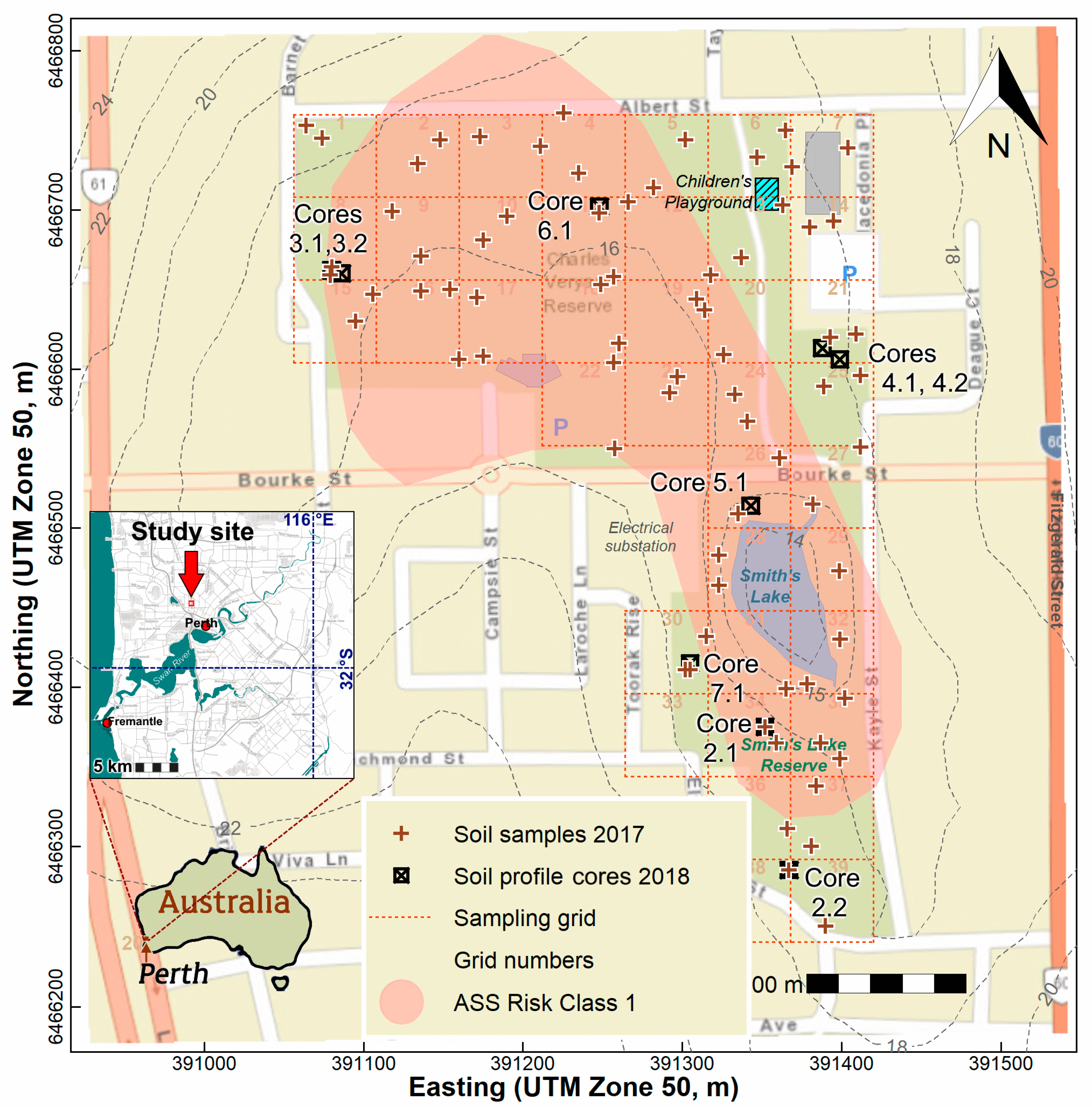
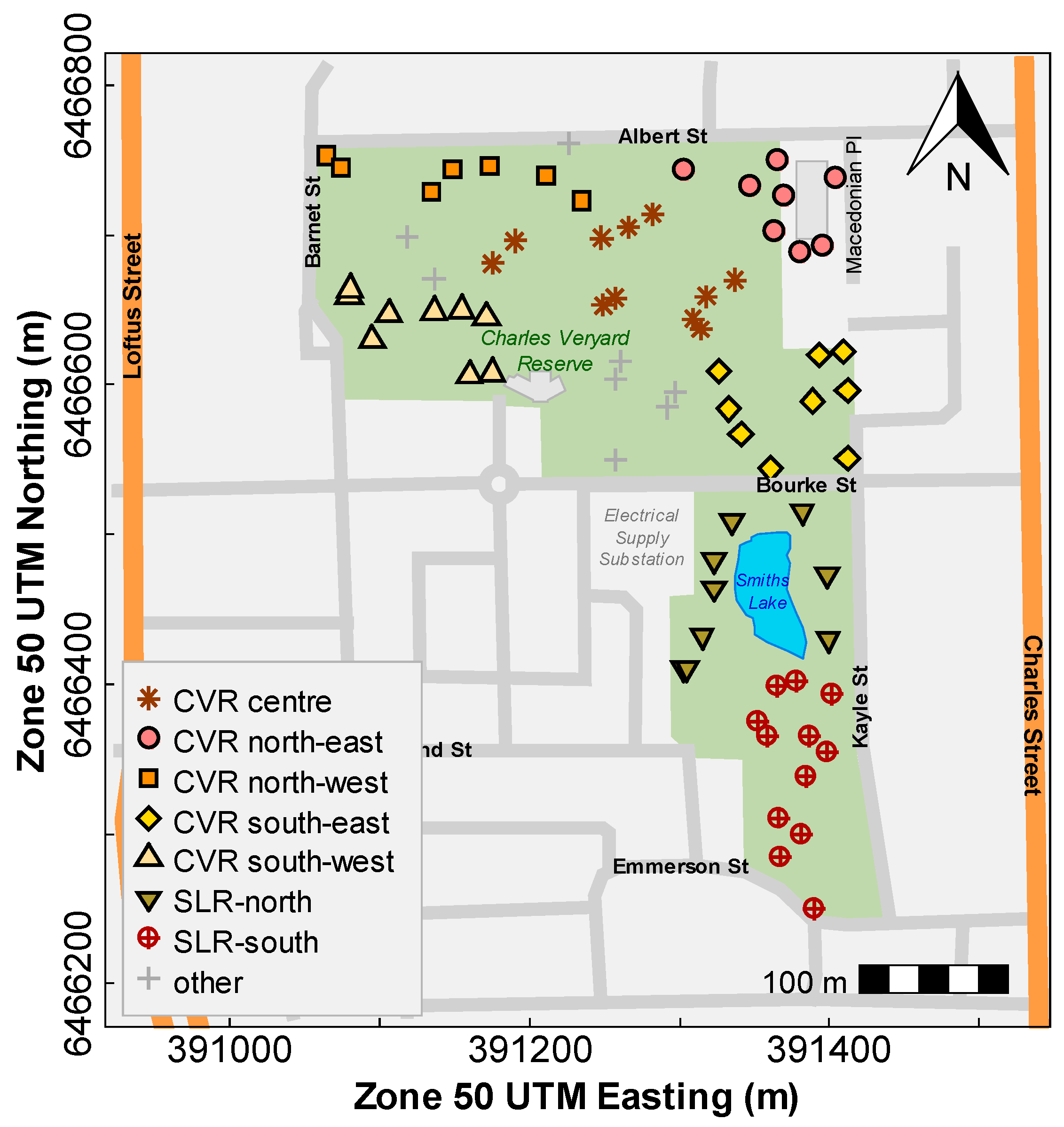
Sampling of soil at Smith’s Lake and Charles Veryard Reserves was conducted on two occasions: in March 2017 (a grid of surface samples) and March 2018 (profile sampling at selected locations). In 2017, surface soil sampling locations were pre-selected prior to sampling using a randomised-within-grid sampling strategy (Figure 1) using a 52 × 52 m grid to maximise site coverage, and two samples per grid square, with the objective of sampling the grassed areas within the Reserves without statistical bias. In the field, preselected sample locations were located using handheld GPS. If randomised sample coordinates were too close to paved surfaces, water, structures, etc., the location was moved by approximately 5 m and the revised coordinates were recorded. For subsequent analysis, the sampling area was divided into zones based on exploratory data analyses (Figure 2).

Surface soil was sampled in cylindrical cores from 0–10 cm depth using a stainless steel corer. Triplicate cores at each location were bulked to achieve a sample mass of ca. 500 g, and stored in zip-lock plastic bags prior to transport back to the laboratory. Soil sample cavities were re-filled with clean soil supplied by the sampling team.

In 2018, a second sampling of soil profiles to up to 100 cm depth was conducted using Garret-style augers. Separate samples were collected for each of eight profiles (Figure 1) in 10 cm depth increments.

Soil samples were air-dried in a laminar air-flow drying cabinet at 40 °C and sieved through a 2 mm aperture prior to analysis.

2.3. Chemical Analysis

The electrical conductivity (EC; proportional to soluble salt content) of soil samples was determined on 1:5 solid: Deionised water suspensions using a calibrated conductivity cell electrode. The pH was measured on the same suspensions using a glass-reference pH electrode after a 2-point buffer calibration [18].

The near-total concentrations of 26 elements (Al, As, Ba, Ca, Cd, Ce, Cr, Cu, Fe, Gd, K, La, Mg, Mn, Mo, Na, Nd, Ni, P, Pb, S, Sr, Th, V, Y, and Zn) were measured on samples by inductively-coupled plasma optical emission spectrometry (ICP-OES) following digestion of soil in concentrated nitric and hydrochloric acids (i.e., aqua regia) at ca. 130 °C [19]. Aqua regia digestion is commonly used to determine environmentally significant concentrations, since it largely excludes elements within the matrices of silicates and other recalcitrant minerals. Before acid digestion, samples were ground to ≲50 µm using ceramic mortars and pestles. Reagent blanks, and grinding blanks composed of acid-washed silica sand, were included in analytical runs to check for contamination. The standard reference stream sediment material STSD-2 [20] was analysed identically to samples to assess analytical accuracy. Measurement precision was assessed using analytical duplicates on ca. 10% of samples.

The lower limits of analytical detection were calculated, where possible, from 3× the standard deviation of multiple reagent blank concentrations [21]. Concentrations lower than mean blank values, or below calculated lower detection limits, or both, were deleted from the dataset.

2.4. Statistical and Numerical Analysis

Data management and transformation of variables was conducted using Excel^® (Version 2016, Microsoft, Redmond, WA, USA) Statistical and graphical analyses of data were performed in the statistical computing environment ‘R’ [22] and associated packages. Skewed variables (identified with the Shapiro-Wilk test for normality) were log₁₀-transformed, or power-transformed based on the Box-Cox algorithm and re-checked for normality.

A general inability of variables to be transformed to yield normal distributions dictated the use of the non-parametric Spearman correlations, and Wilcoxon or Kruskal-Wallis tests for mean comparisons. If Kruskal-Wallis tests showed a significant difference, the R package ‘PMCMR’ [23] was used to apply the post-hoc Conover’s test for pairwise comparisons of mean rank sums. Simple regression models were fitted using the log₁₀-transformed variables. The potentially misleading effects of compositional closure were addressed using transformations to centred log-ratios [24], which were used for principal components analyses. Principal components analyses were conducted using only variables having minimal or no missing observations.

Distribution maps were constructed using the ‘OpenStreetMap’ package [25] with elevation contours interpolated from a dense grid of land elevations from Google [26] generated using the R package ‘googleway’ [27] and interpolated using the R package ‘akima’ [28]. Spatial autocorrelations were assessed using global and local Moran’s I statistics, calculated using the R package ‘lctools’ [29]. Local Moran’s I values showing significant association (p ≤ 0.05) were categorised using high-low notation, based on the point measurement relative to the median and the sign of the Local Moran’s I statistic. Spatial interpolations were achieved using an inverse distance weighting method using the R packages ‘sp’ [30] and ‘gstat’ [31]. Preliminary analysis showed that inverse-distance interpolation gave similar results to simple kriging, but kriging interpolation was not used, based on the requirement of ≥100 observations to generate a reliable experimental variogram [32].

A composite estimate of soil contamination was calculated from the concentrations of As, Cu, Pb, and Zn as the Integrated Pollution Index, IPI [33], shown in Equation (1):

$$\mathrm{IPI}=\left({\sum }_{i=1}^n\left(\frac{{\mathrm{C}}_i}{{\mathrm{S}}_i}\right)\right)/n,$$

(1)

In Equation (1), ∑ means the sum of terms 1 to n, C_i = the measured concentration of th i-th element, S_i = the background concentration of the i-th element, n = the number of elements. The S_i values used (in mg/kg: As = 1.5, Cr = 10, Cu = 2, Pb = 5, Zn = 6) were published ambient background concentrations for the Perth region [34], but this report suggests a zero-background concentration for Ni. In this study 1 mg Ni/kg was used for background, which is the lowest (most conservative) 25th percentile concentration among similar datasets (e.g., [35]).

3. Results

3.1. Bulk Chemical Analyses of Surface Soil

Substantial variability in the concentrations of major elements and basic soil properties (

Table 1. Summary of pH, EC, and major element concentrations in surface (0–10 cm) soil and in vertical soil profile samples at Smith’s Lake and Charles Veryard Reserves. EC and pH were measured in 1:5 solid: deionised water suspensions; element concentrations were measured using aqua regia digestion followed by ICP-OES.

Statistic	pH	EC	Major Element Concentration (mg/kg)
		(µS/cm)	Al	Ca	Fe	K	Mg	Na	P	S
Surface soil (random-in-grid samples, 2017)
Mean	6.92	183	2667	5083	2695	161	425	130	244	309
Std. Dev.	0.63	146	758	7082	939	75.3	285	69	123	186
Minimum	5.28	29.1	396	283	1205	41.1	57.3	27.8	18.5	43
Median	6.84	151	2637	1813	2530	150	347	118	221	280
Maximum	8.63	835	4722	30,472	5640	424	1471	410	596	1293
No of valid analyses	73	58	68	68	68	68	68	68	68	68
Soil profiles to ≤ 100 cm (2018)
Mean	7.67	116	3214	11,061	4430	173	548	148	146	518
Std. Dev.	1.96	61	2168	14,254	3358	100	505	100	137	334
Minimum	4.48	7.92	149	38	218	26	14	11	4	48
Median	7.98	83	2880	7894	3593	134	450	127	140	293
Maximum	9.40	860	10,353	57,265	22,180	655	2365	513	386	4929
No of valid analyses	84	83	85	85	85	85	85	85	85	83

), including potential trace element contaminants (

Table 2. Summary of minor/trace element concentrations in surface (0–10 cm) soil and in vertical soil profile samples at Smith’s Lake and Charles Veryard Reserves. Element concentrations were measured using aqua regia digestion followed by ICP-OES.

	Concentrations (mg/kg)
Statistic	As	Ba	Cd	Cr	Cu	Mn	Mo	Ni	Pb	Sr	V	Zn
Surface soil (random-in-grid samples, 2017)
Mean	2.58	15.7	0.11	7.33	8.69	39.5	0.23	2.58	25.7	27.8	5.38	55.2
Std. Dev.	1.09	7.38	0.1	2.29	11	23.7	0.1	2.83	31.7	40.3	1.66	56.5
Minimum	0.9	6.2	0.02	1.17	2.13	2.68	0.07	0.25	3.23	2.4	1.28	5.59
Median	2.3	14.5	0.08	7.32	5.25	34.5	0.22	2.13	14.7	10.3	5.35	34.7
Maximum	5.86	41.7	0.66	13.8	67.5	127	0.6	21.3	174	186	10.6	304
No of analyses	68	68	62	68	68	68	68	68	68	68	68	68
No > HIL(C) 1	0	-	0	0	0	0	-	0	0	-	-	0
No > EIL 3	0	0	0	0	0	0	-	0	0	-	0	3
Soil profiles to ≤ 100 cm (2018)
Mean	3.28	25.2	0.18	9.09	41.4	28.0	0.48	5.39	72.7	62.3	8.38	117
Std. Dev.	2.79	26.2	0.31	6.96	66.6	21.7	0.81	20.7	98.8	85.1	5.56	191
Minimum	0.6	1.9	0.01	0.2	2.8	1.5	0.06	0.6	3.5	1.8	0.3	3.3
Median	2.5	15.3	0.06	8.1	15.1	24.3	0.21	1.97	32.2	34.3	7.2	43.2
Maximum	14.6	139	1.6	34.4	356	97.9	5.63	181	568	391	30.4	1155
No of analyses	83	85	79	85	67	85	78	75	84	80	85	84
No > HIL(C) 1	0	-	0	0	0	0	-	0	0	-	-	0
No > EIL 3	0	0	0	0	8	0	-	1	1	0	0	14

¹ Health Investigation Level C (Recreational) [36]; ³ Ecological Investigation Level (interim urban) [37].

), was observed in surface soils at Smith’s Lake and Charles Veryard Reserves. In most cases, the maximum concentrations were at least five times the minima. Much greater variability was observed for calcium (Ca, maximum/minimum ≈ 108); cadmium (Cd), copper (Cu), magnesium (Mg), manganese (Mn), neodymium (Nd), nickel (Ni), phosphorus (P), lead (Pb), sulfur (S), strontium (Sr), and zinc (Zn) all had maximum/minimum ratios between 20 and 90. Soluble salt content measured by EC showed a maximum/minimum ratio of ≈29, and there was a relatively large, ≈3.4 units range in pH across the Reserves. Except for zinc, which exceeded the interim Ecological Investigation Level (EIL; National Environment Protection Council, 1999) in three samples, no other soil thresholds were exceeded by any element (Table 2).

3.2. Spatial Distributions in Surface Soil

The measurements of primary interest (pH, EC, Al, As, Ca, Cu, Fe, Pb, Zn) generally showed significant overall spatial patterns across the study area, shown by p values ≤ 0.05 for Global Moran’s I. The exceptions were Al, Ca, Cr, and Ni for which the Global Moran’s I values were close to zero (

Table 3. Global Moran’s I, p-values simulated by Monte-Carlo randomization, and information on local spatial autocorrelation for the variables of principal interest in surface soil at Smith’s Lake and Charles Veryard Reserves. Variables except pH were log₁₀-transformed before calculation. IPI is integrated pollution index (Equation (1)).

Variable	Moran’s I	p-Value	Number of Points with Significant Local Moran’s I	Location (and Number of Points) of High-High LOCAL Moran’s I Clusters a
pH	0.440	>0.001	13	CVR-SW (2), CVR-SE (3), SLR-S (4)
EC	0.157	0.035	7	SLR-S (3)
Al	0.014	0.691	4	CVR-SE (2) b
As	0.228	0.002	6	CVR-SE (4)
Ca	0.074	0.254	6	SLR-S (2)
Cr	0.016	0.672	4	CVR-SE (1)
Cu	0.331	>0.001	9	CVR-NE (3), CVR-SE (5)
Fe	0.142	0.044	11	CVR-NE (1), CVR-SE (5)
Ni	0.047	0.426	5	CVR-SE (1) b
Pb	0.324	>0.001	11	CVR-SE (5), SLR-N (2)
Zn	0.209	0.004	10	CVR-NE (2), CVR-SE (4)
IPI	0.257	>0.001	10	CVR-NE (1), CVR-SE (5)

^a CVR is Charles Veryard Reserve; SLR is Smiths Lake Reserve; NE is north-east; NW is north-west; SE is south-east; SW is south-west; N is north; S is south; E is east; ^b not associated with main CVR-SE cluster.

). The spatial patterns and clusters of points with significant local autocorrelation are shown in Figure 3, Figure 4, Figure 5 and Figure 6, and summarised in Table 3.

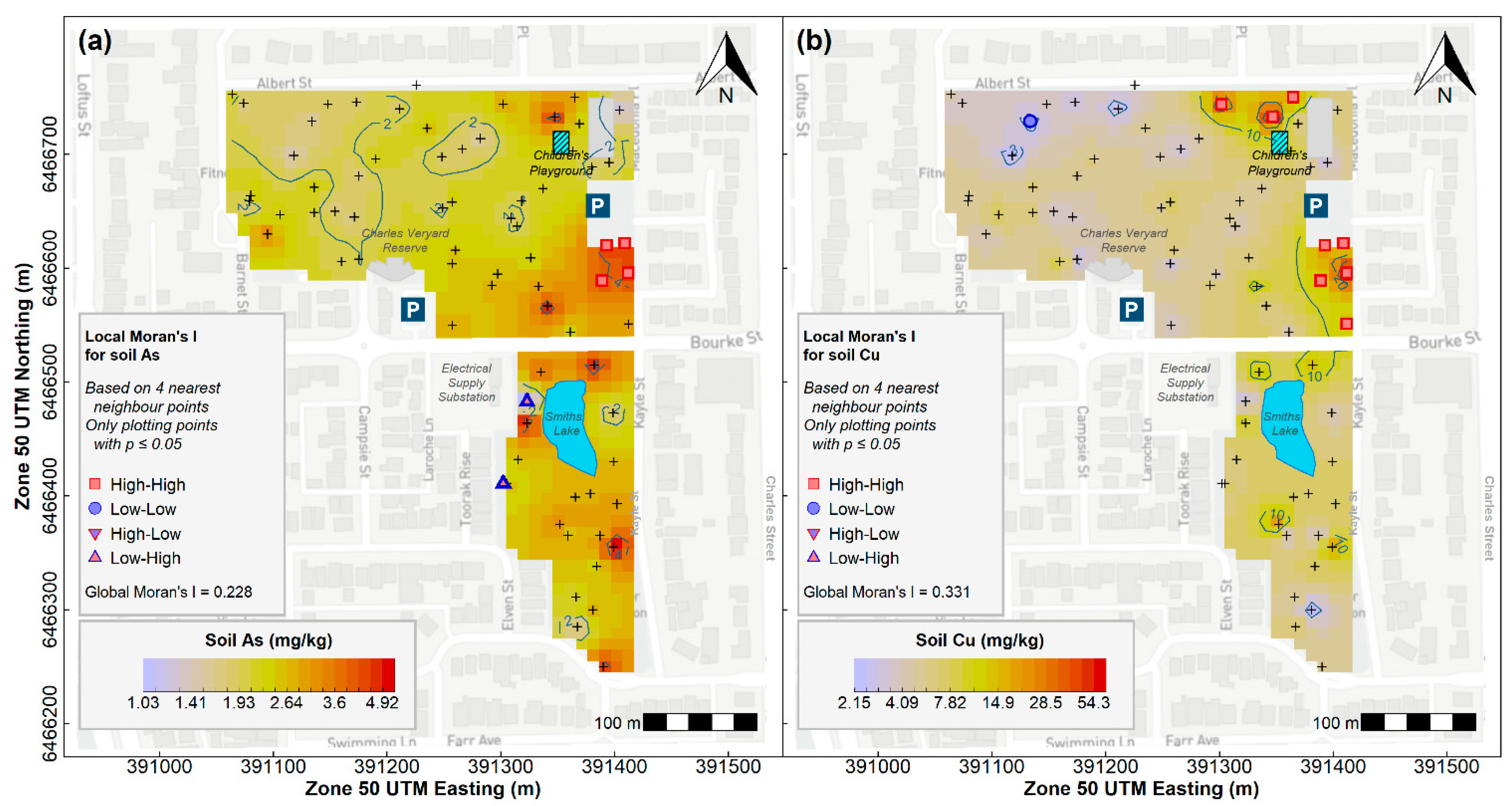
Arsenic (As) showed a broad concentration peak in soil in the south-east of Charles Veryard Reserve, with scattered local maxima in a few other locations (Figure 3). The As peak in the south-east of Charles Veryard Reserve was co-located with samples having significant (p ≤ 0.05) high-high local Moran’s I. Two points in Smith’s Lake Reserve had significant low-high local Moran’s I (i.e., isolated low As concentrations).

Copper (Cu) showed peaks in the north-east and south-east of Charles Veryard Reserve, with no other obvious maxima (Figure 3). Samples in both peaks in Cu concentration were significantly spatially autocorrelated (high-high, local Moran’s I p ≤ 0.05). One point in north-west Charles Veryard Reserve had significant low-high local Moran’s I (i.e., an isolated low Cu concentrations).

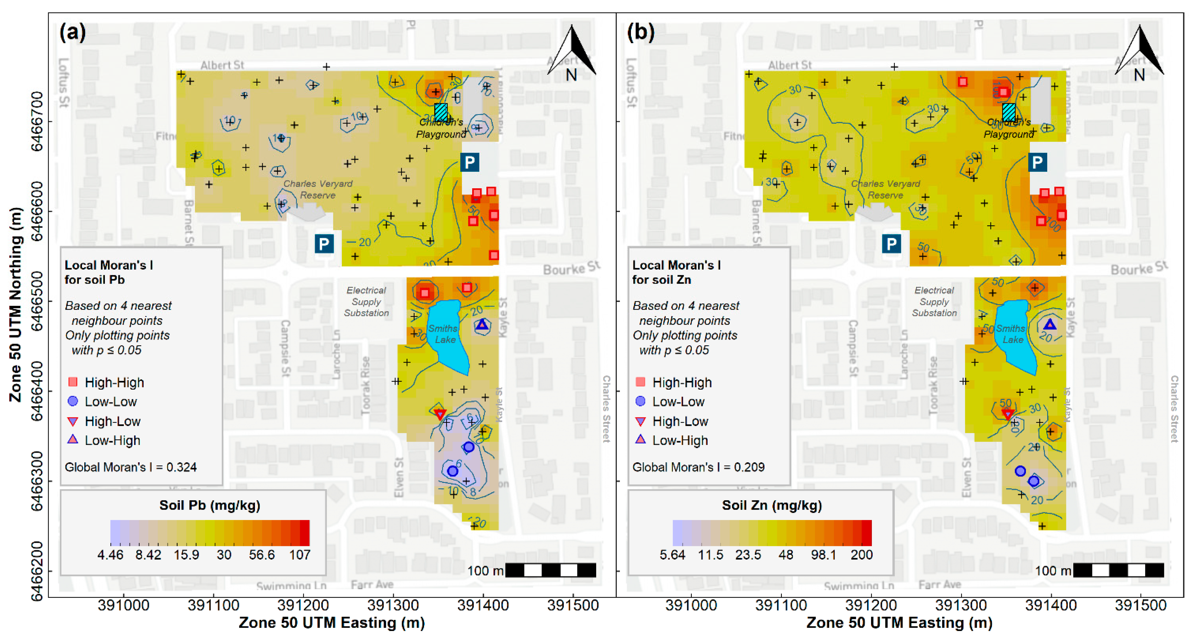
Lead (Pb) showed peaks in concentration in soil in the south-east of Charles Veryard Reserve and the north of Smith’s Lake Reserve, with scattered local maxima in Pb concentration in a few other locations (Figure 5). The Pb peak in the south-east of Charles Veryard Reserve was co-located with samples having significant (p ≤ 0.05) high-high local Moran’s I. A broad area of low Pb concentrations in Smith’s Lake Reserve coincided with significant (p ≤ 0.05) low-low local Moran’s I, and instances of significant high-low and low-high local Moran’s I values represented isolated high and low Pb concentrations.

Zinc (Zn) showed peaks in the north-east and south-east of Charles Veryard Reserve, with a few other subtle maxima (Figure 5). Samples in both clear peaks in Zn concentration were significantly spatially autocorrelated (high-high, local Moran’s I p ≤ 0.05). An area of low Zn concentrations in Smith’s Lake Reserve coincided with significant (p ≤ 0.05) low-low local Moran’s I. Similar to Pb, instances of significant high-low and low-high local Moran’s I values in Smith’s Lake Reserve represented isolated high and low Zn.

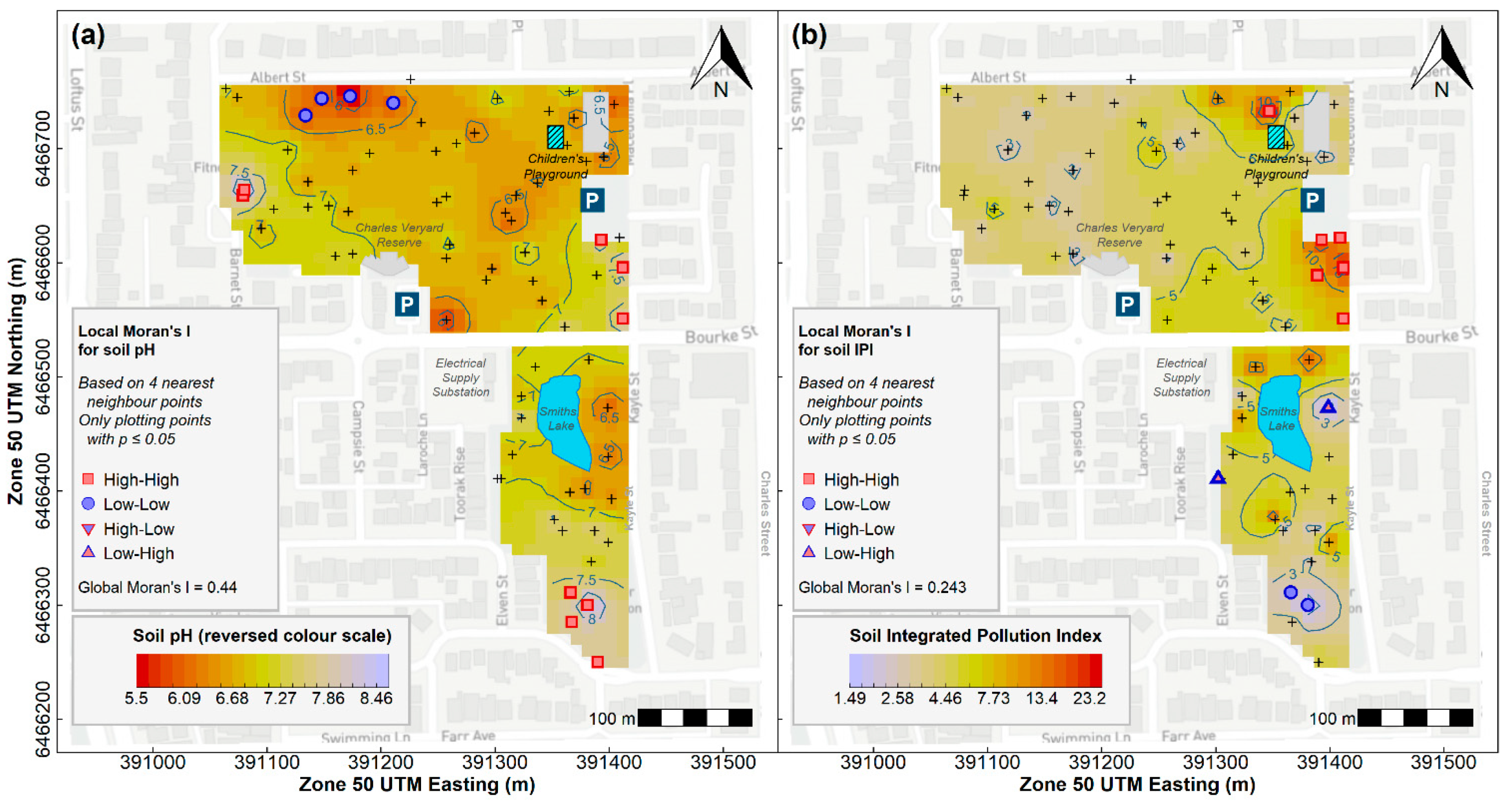
Soil pH showed a cluster of lower values in the north-west of Charles Veryard Reserve with significant low-low spatial autocorrelation (Moran’s I p ≤ 0.05). In contrast, significant clusters of higher pH values were present in the west of Charles Veryard Reserve, the south-east of Charles Veryard Reserve, and the south of Smith’s Lake Reserve (Figure 6).

Finally, the derived Integrated Pollution Index (IPI) had a maximum in the south-east of Charles Veryard Reserve, with a minor maximum in the north-east (Figure 6). A cluster of samples in the south-east IPI peak were significantly spatially autocorrelated (high-high, local Moran’s I p ≤ 0.05). An isolated low IPI value (low-high local Moran’s I, p ≤ 0.05) was present to the east of Smith’s Lake.

A comparison of mean values of the variables of interest between samples from the different zones in Figure 2 reinforced the qualitative results from spatial interpolation (

Table 4. Comparison of pH, EC (1:5 soil: water extract), element concentrations, and IPI in distinct Zones of Smith’s Lake (SLR) and Charles Veryard (CVR) Reserves. Mean values in a row are different if no superscript letters are shared (p ≤ 0.05, Conover’s pairwise test with Holm’s correction).

Variable	P (K-W) 1	Mean in Each Zone 2
		CVR- Centre	CVR-NE	CVR-NW	CVR-SE	CVR-SW	SLR-N	SLR-S	Other
pH	0.0001	6.58 a	6.65 ab	6.24 a	7.34 bc	7.35 bc	6.88 abc	7.38 c	6.66 abc
EC	0.013	155 ab	90.7 ab	273 a	159 ab	232 a	68.1 b	265 ab	143 ab
Al	0.028	2530 ab	2857 ab	2285 a	3373 b	2621 ab	1960 ab	3011 ab	2489 ab
As	0.004	1.91 a	2.46 ab	1.96 a	3.79 b	2.17 a	2.99 ab	3.04 ab	2.38 ab
Ca	0.004	1766 abc	3511 abc	4534 abc	6710 abc	7472 ab	3570 ac	11,450 b	1343 c
Cr	0.020	6.98 ab	8.47 ab	6.62 a	9.42 b	7.18 ab	5.85 ab	7.51 ab	6.20 a
Cu	0.010	5.10 ab	16.7 ab	3.57 a	17.6 b	5.36 ab	8.43 ab	8.34 ab	4.52 ab
Fe	0.041	2377 ab	2936 ab	2071 a	3623 b	2418 ab	2680 ab	2861 ab	2535 ab
Ni	0.300	ns	ns	ns	ns	ns	ns	ns	ns
Pb	0.043	11.7 a	31.2 ab	15.4 ab	56.9 b	15.3 ab	47.8 ab	15.7 a	16.5 ab
Zn	0.255	ns	ns	ns	ns	ns	ns	ns	ns

¹ Overall p-values from Kruskal-Wallis test; ² CVR is Charles Veryard Reserve; SLR is Smiths Lake Reserve; NE north-east; NW north-west; SE south-east; SW south-west; N north; S south.

). The highest mean values for several potential contaminants (As, Cr, Cu, and Pb) were observed in the south-east of Charles Veryard Reserve (no significant effect of sampling zone was found for Ni or Zn).

3.3. Relationships between Soil Elements

Several significant positive correlations existed between elements across the soil data from Charles Veryard and Smith’s Lake Reserves (Table S1, Supplementary Material). Calcium, Mg and Sr were very highly correlated (r = 0.80–0.96), and Ca and Sr were the only elements significantly correlated (r = 0.66) with pH. The major elements Na, K, and Mg were all highly correlated (r ≥ 0.7), as were P, K, Mn, and S. High correlations also existed between iron (Fe) and As, Ba, Cu, Pb, and V. Many potential contaminants were also highly correlated with one another, e.g.,: Cu with Ba, Pb, and Zn; Pb with Cd, Cu, and Zn; Cr with V.

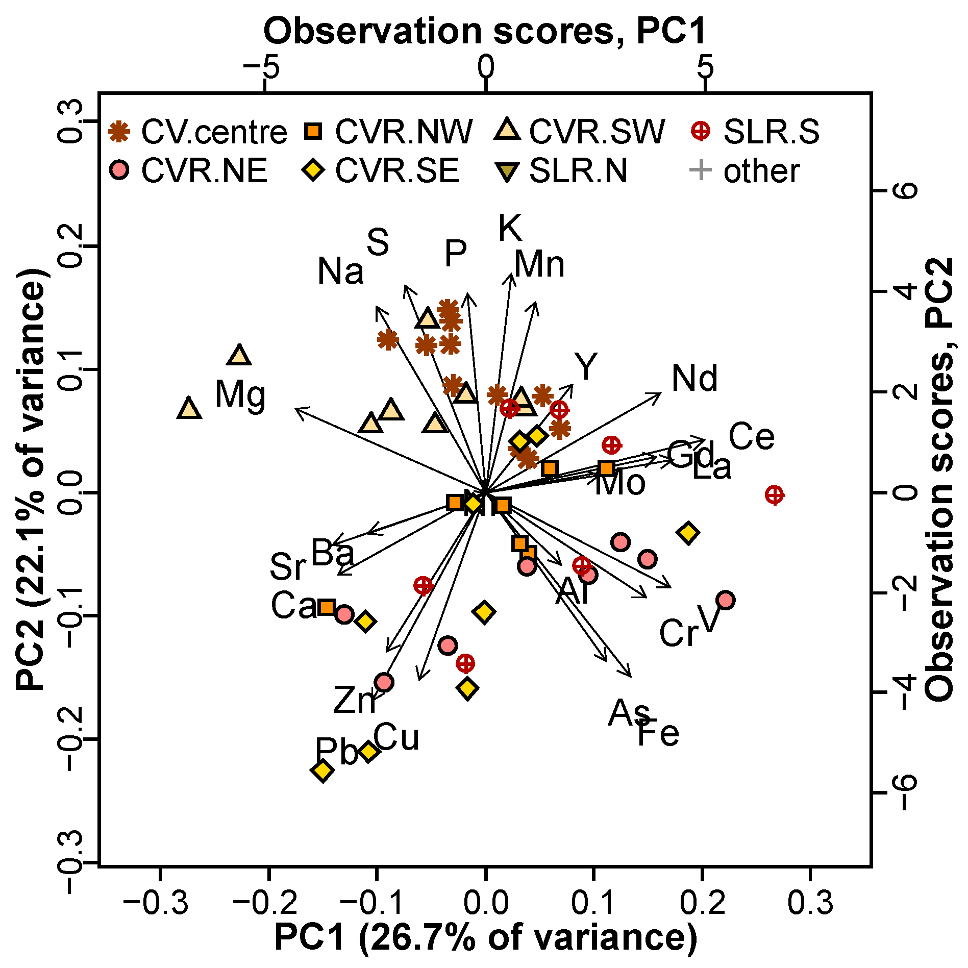
Principal components analysis (Figure 7) showed grouping of Cu, Pb, and Zn in PC1-PC2 space, associated with some of the samples from north-east and south-east where peak concentrations of these elements were observed (Figure 3 and Figure 5). Arsenic plots at similar values of PC2, but has an association with Fe and Cr at small positive PC1 values. No obvious element associations were observed using PCA for Ni. The principal components analysis also identifies an association of Ca with Sr and Ba, an association of nutrient elements (S, P, K) with the central Charles Veryard Reserve samples, and clustering of rare-earth and related elements (Ce, Gd, La, Nd, Y). Additional results derived from principal components analysis are available in Tables S2–S4 in the Supplementary Materials.

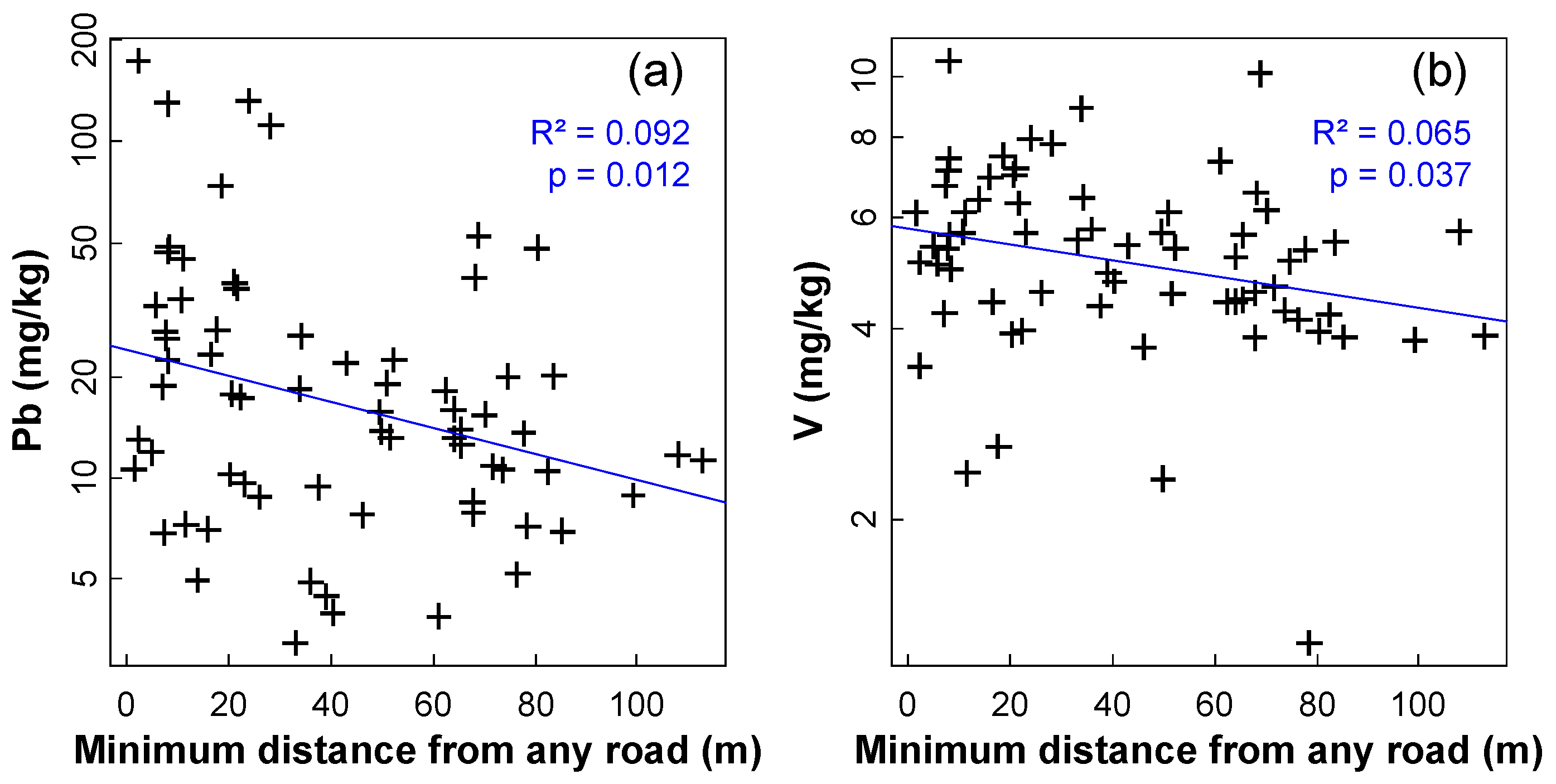
In surface soil, there was a weak negative relationship between lead and vanadium concentrations and minimum (Euclidean) distance from any road surrounding or bisecting the reserves (Figure 8). No other contaminant of primary interest showed a significant trend in relation to distance from roads.

3.4. Depth Distributions of As, Cr, Cu, Ni, Pb, and Zn

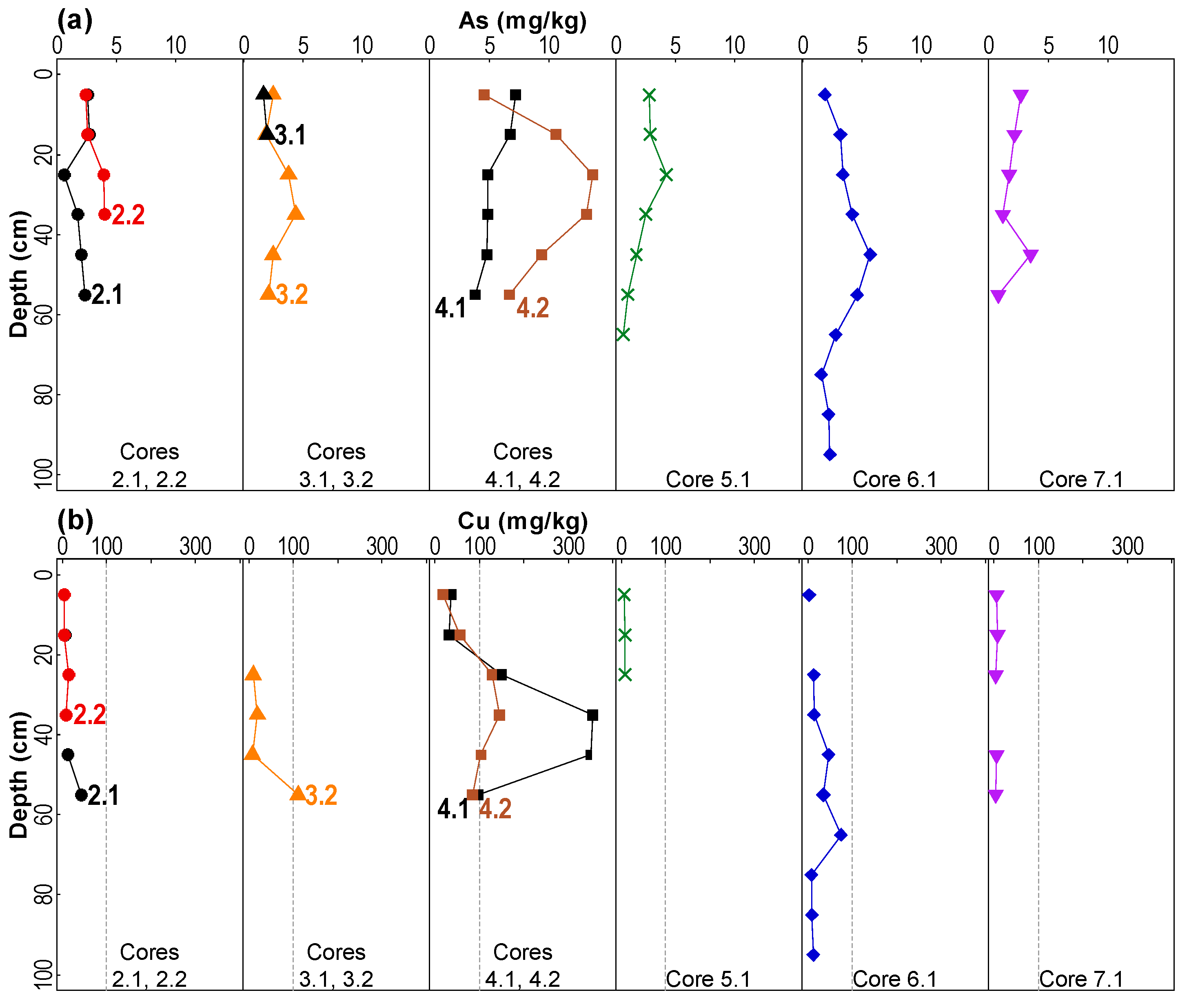
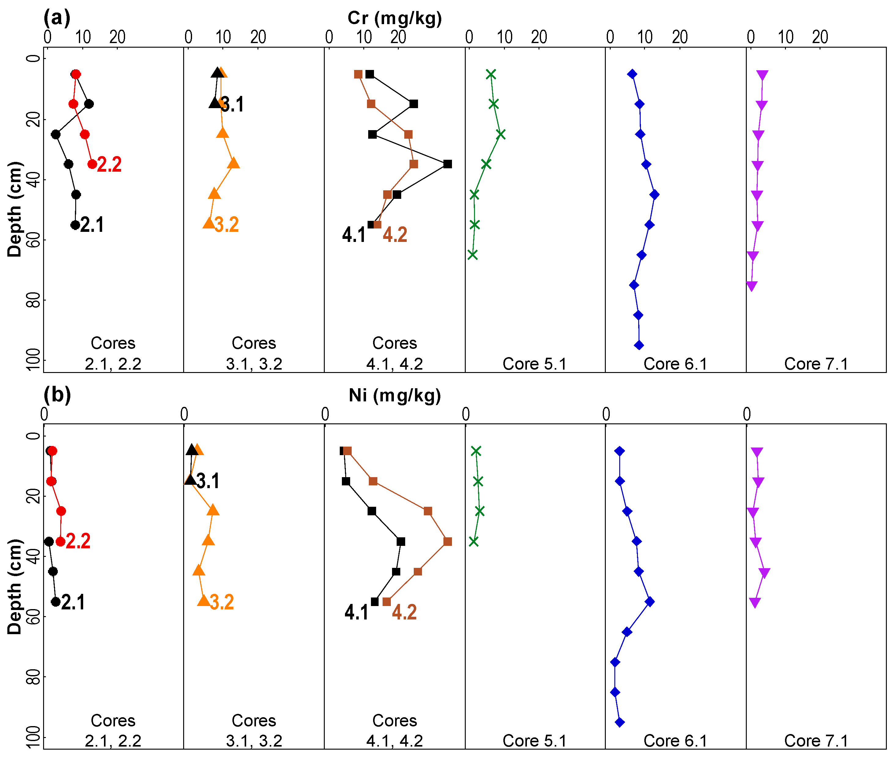
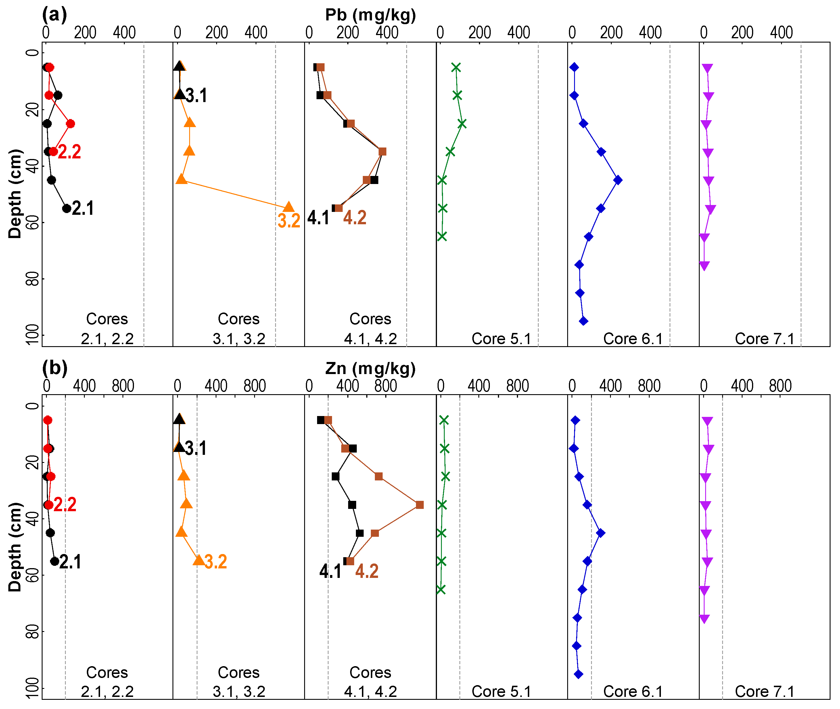
Depth profile plots for As, Cr, Cu, Ni, Pb, and Zn are presented in Figure 9, Figure 10 and Figure 11. Depth profiles of As, Cr, Cu, Ni, Pb, and Zn frequently showed maximum concentrations in subsurface soil samples. High maximum concentrations of Pb (376 mg/kg) and Zn (1155 mg/kg) were measured at 30–40 cm in core 4.2 (Figure 11), on the eastern side of Charles Veryard Reserve south of the Macedonia Place car park. Core 3.2 also contained 568 mg/kg Pb at 50–60 cm. Core 4.2 also contained the maximum concentration of As (14 mg/kg at 20–30 cm), Cd, Mn, and Ni. The greatest concentration of Cu (356 mg/kg) was observed in the adjacent core 4.1 (Figure 9).

There was a tendency for pH to increase with increasing depth, and EC to decrease with increasing depth, and the trends in Fe with depth were very similar to those for As (Figure S1, Supplementary Material).

4. Discussion

4.1. Concentrations of Potential Contaminants

Surface soils in the Charles Veryard and Smith’s Lake Reserves were largely uncontaminated with any of the elements measured. No potential contaminant in surface soil or subsoil exceeded any relevant human health guideline for recreational/public open space land use (Table 2). This may reflect rehabilitation of the site to parkland using techniques as simple as covering with clean fill, which is known to suppress the surface expression of soil contamination [38]. In surface soil, the only element to exceed a guideline value was Zn, which had concentrations greater than the 200 mg/kg EIL threshold [37] in the southeast (two samples) and northeast (one sample) of Charles Veryard Reserve. More subsoil than surface soil samples exceeded EIL thresholds (Table 2).

The exceedance of EIL guideline values by Zn in a few surface soil samples and several subsoil samples in the eastern zones of Charles Veryard Reserve (Figure 9, Figure 10 and Figure 11) reflects the common occurrence of zinc in urban environments, especially building materials and road traffic, and export of Zn into soil environments [39,40]. Very few toxicological studies exist on the effects of zinc on typical sports turf plants or the microbial ecology in these environments; the likelihood that this Zn represents anthropogenic additions means that the bioavailability of Zn would therefore also be expected to be greater than for native soil Zn [36,41].

4.2. Spatial Patterns of Potential Contaminants in Surface Soil

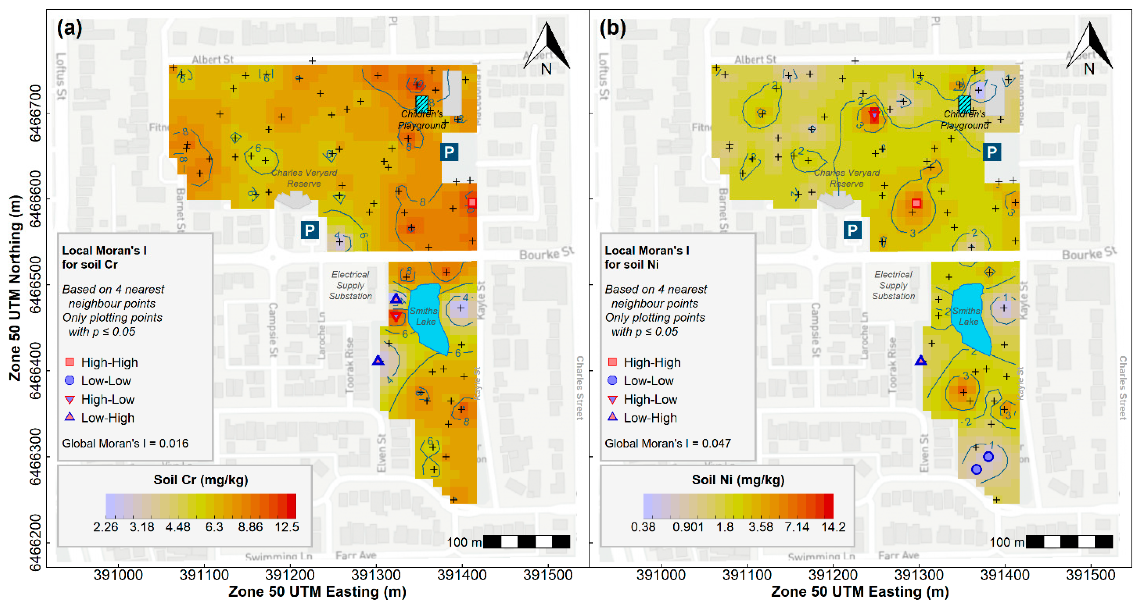
Although the incidence of actual surface soil contamination was low at Charles Veryard and Smith’s Lake Reserves, the zone in which most enrichment of potential contaminants (As, Cr, Cu, Pb, and Zn) occurred coincided with the greatest subsoil concentrations of these elements (Figure 9, Figure 10 and Figure 11). This was the CVR-SE zone, in which the greatest number of point-variable combinations had significant high-high local Moran’s I statistics (Table 3), confirming the visualizations generated by inverse-distance interpolation (Figure 3, Figure 4, Figure 5 and Figure 6). Based on these analyses, the south-east corner of Charles Veryard reserve, an area approximately 40 m N-S and 20 m E-W (ca. 800 m²), is contaminated with As, Cu, Pb, and Zn, a finding supported by the Integrated Pollution Index (Figure 6b). Based on a single sample with significant high-high Local Moran’s I, and weak evidence of subsoil enrichment, Cr contamination may also be present in this location. However, the Global Moran’s I statistics for Cr and Ni could not reject the null hypothesis of no spatial pattern, and no local Moran’s I values were significant for Ni, so it is unlikely that either Cr or Ni have been added by contamination processes at the study site. Both Cr and Ni also had significant isolated high concentrations (significant high-low local Moran’s I; Figure 4)) which were not co-located; no isolated high concentrations were observed for As, Cu, Pb, or Zn.

The CVR-SE zone was the location of soil cores showing the greatest concentrations of As, Cr, Cu, Ni, and Zn, and the most exceedances of each element’s ecological investigation limit (EIL) concentrations (Figure 9, Figure 10 and Figure 11). Pb concentrations in subsoil at this location were also high, although the greatest concentration occurred in Core 3.2 in the west of Charles Veryard Reserve. The co-location of surface soil contamination identified by spatial analysis with subsoil contaminant maxima confirms the south-east Charles Veryard Reserve area as the only location of significant contamination.

4.3. Associations of Potential Contaminants

Despite the minimal surface soil contamination, the identification of distinct soil zones based on their geochemical properties (Figure 3, Figure 4, Figure 5 and Figure 6) suggested that these different zones may represent the signatures of past activities or construction at the Charles Veryard and Smith’s Lake Reserves. The element associations identified in the soil zones were supported by the Principal Components Analysis (Figure 7).

The associations identified by Principal Components Analysis are consistent, and also make geochemical sense. The nutrient elements K, P, and S probably represent a common source from historical horticulture [42]. The grouping of Ca, Mg, Sr, and Ba includes elements which are all commonly associated with carbonates and/or cement-based materials [35]. The metal contaminants Cu, Zn, and Pb often have a common source such as building materials or roads and traffic [43]. Finally, Fe, As, Cr, and V reflect the commonly-observed associations of As, Cr, and V with iron oxides in soils [44], and Cr and V are used with Fe in manufacture of some steel products [45].

The association of Cu, Pb, and Zn in PC1-PC2 space, and to some extent As and Cr in the second principal component dimension, validated the calculation of the Integrated Pollution Index (IPI) from these elements. The IPI values are unusually high (range 6–28), reflecting the somewhat low values used for background concentrations. Reliable background concentrations for trace elements in soils of the Swan Coastal Plain around metropolitan Perth are still subject to uncertainty and obtaining these should be a priority for local research.

The low pH and low concentrations of many elements in the north-west of Charles Veryard Reserve most likely reflect a very sandy (i.e., poorly buffered) soil material which has been subject to minor acidification. This acidification may have originated from historical or recent disturbance of the underlying peaty acid sulfate soil material (e.g., by light pylon installation), given the classification of much of the Charles Veryard and Smith’s Lake Reserves area as being high to moderate risk of acid sulfate soil within 3 m of the land surface (Figure 1).

Elevated concentrations of Cu, Pb, and Zn in the north-east of Charles Veryard Reserve most likely represent contributions from construction (the Macedonian Centre, buildings on Albert Street) and possibly road traffic [39,46]. A road traffic origin for Pb is supported by the significant negative relationship of Pb with distance from roads (Figure 8). Construction and historical waste disposal sources are likely to have contributed Cu, and Pb to the south-east of Charles Veryard Reserve. The Charles Veryard Reserve south-east soil zone also has elevated pH, Al and Fe, however, so background concentrations may be naturally higher due to greater clay and/or iron oxide content of soils [44]. The greater concentrations of arsenic are most likely due to retention on Fe oxides, since there are no obvious sources of contamination and As concentrations are generally low. The greater concentrations of Al and Fe may themselves represent contamination from disposal of metalliferous wastes.

Soil in the south-west of Smith’s Lake Reserve is characterized by higher pH and concentrations of Ca, Sr, Na, and P (and possibly K, S, and Mn). The high pH and elevated Ca and Sr are likely to represent additions of limestone or cement-based building materials [47]. Such additions are plausible given the relatively recent (2008) demolition of the Len Fletcher Sports Pavilion in the south of Smith’s Lake Reserve.Enrichment with the nutrient elements P, K, and S, and also Na, may reflect historical market gardening at the site and associated use of fertilisers, or organic amendments such as composts or manures [1].

The weak but significant trend in lead and vanadium concentrations as a function of distance from roads (Figure 8) suggests that road traffic was a significant source of these elements, in agreement with previous studies [48]. Since leaded fuels are no longer used in Australia and numerous other countries, the inputs of Pb are likely to represent a historical legacy of Pb accumulation in roadside soils. The abrasion of road surfaces by traffic is a potential source of vanadium from bituminous materials used as asphalt binders [49].

Concentrations of Cu, Pb, and Zn in soil profiles exceeded Ecological Investigation Limits (EILs) in several samples, especially for Zn (Figure 9 and Figure 11). Most of these higher concentrations, however, were in deeper subsoil samples, so the risk to biota (mainly plant and microbial uptake) would therefore be expected to be minimal.

The existence of subsoil maximum concentrations at some locations may represent burial of waste material or drain sediment, or an evaporation/redox front resulting in accumulation of some elements. Given that that waste disposal at the Smith’s Lake and Charles Veryard Reserves site is known to have been widespread [50,51], waste material would seem the most likely source. The relatively high subsoil concentrations of trace elements may represent a health risk, for example if dust is generated during excavation [52]. The potential risk should be considered in the context of a children’s playground adjacent to the most contaminated surface soils and soil profiles.

5. Conclusions

An important conclusion from the initial concentration data is that the surface soil and subsoil sampled in this study at Smith’s Lake and Charles Veryard Reserves is not contaminated with As, Cr, Cu, Ni, Pb, or Zn levels of concern from a human health perspective. There was, however, multiple exceedance of ecological investigation trigger limits (EIL) for Zn in surface soil and Cu, Pb, and Zn in subsoil. The spatial analysis showed that, on the basis of global and local Moran’s I, distributions of most elements were not random but showed clustering. In line with the initial hypothesis, this significant clustering of adjacent higher concentrations in surface soil allowed identification of a specific area which, at the scale of sampling design, represented inputs from a point source of As, Cu, Pb, and Zn. At this site, the specific area of surface soil contamination was co-located with the most significant subsoil contamination, but this may not be a general result.

The combination of multivariate geochemical analysis with spatial information allowed both identification of realistic associations of elements, including potential contaminants. In particular, there was a consistent association of the dominant contaminants (Cu, Pb, and Zn) in the south-east of Charles Veryard Reserve which could be deduced from univariate spatial autocorrelation analysis, a composite contamination index (IPI), and multivariate principal components analysis.

In this study, the location and significance of potential contamination in the soil of urban public open space has been assessed thoroughly by measurement of multiple parameters, and rigorous spatial and statistical analysis. It is recommended that any such study uses a similar approach if soil contamination is suspected, especially given the global tendency for urban populations to increase and for redevelopment of, and increased population density in, inner-city precincts.

References

- Demiguel, E.; Degrado, M.J.; Llamas, J.F.; Martindorado, A.; Mazadiego, L.F. The overlooked contribution of compost application to the trace element load in the urban soil of Madrid (Spain). Sci. Total Environ. 1998, 215, 113–122. [Google Scholar] [CrossRef]
- Chen, T.B.; Wong, J.W.C.; Zhou, H.Y.; Wong, M.H. Assessment of trace metal distribution and contamination in surface soils of Hong Kong. Environ. Pollut. 1997, 96, 61–68. [Google Scholar] [CrossRef]
- Gaw, S.K.; Wilkins, A.L.; Kim, N.D.; Palmer, G.T.; Robinson, P. Trace element and ΣDDT concentrations in horticultural soils from the Tasman, Waikato and Auckland regions of New Zealand. Sci. Total Environ. 2006, 355, 31–47. [Google Scholar] [CrossRef]
- Tarzia, M.; De Vivo, B.; Somma, R.; Ayuso, R.A.; McGill, R.A.R.; Parrish, R.R. Anthropogenic vs. natural pollution: An environmental study of an industrial site under remediation (Naples, Italy). Geochem. Explor. Environ. Anal. 2002, 2, 45–56. [Google Scholar] [CrossRef]
- Appleyard, S.; Wong, S.; Willis-Jones, B.; Angeloni, J.; Watkins, R. Groundwater acidification caused by urban development in Perth, Western Australia: Source, distribution, and implications for management. Aust. J. Soil Res. 2004, 42, 579–585. [Google Scholar] [CrossRef]
- Orndorff, Z.W.; Daniels, W.L.; Fanning, D.S. Reclamation of acid sulfate soils using lime-stabilized biosolids. J. Environ. Qual. 2008, 37, 1447–1455. [Google Scholar] [CrossRef]
- Grundy, S.L.; Bright, D.A.; Dushenko, W.T.; Dodd, M.; Englander, S.; Johnston, K.; Pier, D.; Reimer, K.J. Dioxin and furan signatures in northern Canadian soils: Correlation to source signatures using multivariate unmixing techniques. Chemosphere 1997, 34, 1203–1219. [Google Scholar] [CrossRef]
- Riemann, U. Impacts of urban growth on surface water and groundwater quality in the City of Dessau, Germany. In Impacts of Urban Growth on Surface Water and Groundwater Quality; Ellis, B., Ed.; IAHS-AISH Publication No. 259; International Association of Hydrological Sciences Press: Wallingford, UK, 1999; pp. 307–314. [Google Scholar]
- Liu, E.; Yan, T.; Birch, G.; Zhu, Y. Pollution and health risk of potentially toxic metals in urban road dust in Nanjing, a mega-city of China. Sci. Total Environ. 2014, 476–477, 522–531. [Google Scholar] [CrossRef]
- Henderson, F.M.; Xia, Z.G. SAR applications in human settlement detection, population estimation and urban land use pattern analysis: A status report. IEEE Trans. Geosci. Remote Sens. 1997, 35, 79–85. [Google Scholar] [CrossRef]
- Huo, X.N.; Zhang, W.W.; Sun, D.F.; Li, H.; Zhou, L.D.; Li, B.G. Spatial pattern analysis of heavy metals in Beijing agricultural soils based on spatial autocorrelation statistics. Int. J. Environ. Res. Public Health 2011, 8, 2074–2089. [Google Scholar] [CrossRef] [Green Version]
- Anselin, L. Local Indicators of Spatial Association—LISA. Geogr. Anal. 1995, 27, 93–115. [Google Scholar] [CrossRef]
- Hojati, S. Use of spatial statistics to identify hotspots of lead and copper in selected soils from north of Khuzestan Province, southwestern Iran. Arch. Agron. Soil Sci. 2019, 65, 654–669. [Google Scholar] [CrossRef]
- Zhang, C.; Luo, L.; Xu, W.; Ledwith, V. Use of local Moran’s I and GIS to identify pollution hotspots of Pb in urban soils of Galway, Ireland. Sci. Total Environ. 2008, 398, 212–221. [Google Scholar] [CrossRef] [PubMed]
- City of Vincent. Thematic History; City of Vincent: Leederville, WA, Australia, 2008.
- Claise Brook Catchment Group. Restoration of Smith’s Lake. Available online: http://www.cbcg.org.au/projects_smiths.html (accessed on 31 October 2017).
- Western Australian Land Information Authority. Landgate Map Viewer Plus. Available online: https://maps.landgate.wa.gov.au/maps-landgate/registered/. https://www0.landgate.wa.gov.au/maps-and-imagery/imagery/aerial-photography/aerial (accessed on 29 June 2021).
- Rayment, G.E.; Lyons, D.J. Soil Chemical Methods—Australasia; CSIRO Publishing: Clayton, VIC, Australia, 2010. [Google Scholar]
- U.S. EPA. Method 3050B: Acid digestion of sediments, sludges, and soils test. In Methods for Evaluating Solid Waste, Physical/Chemical Methods; EPA Publication SW-846; U.S. EPA: Washington, DC, USA, 2007. [Google Scholar]
- Lynch, J. Additional provisional elemental values for LKSD-1, LKSD-2, LKSD-3, LKSD-4, STSD-1, STSD-2, STSD-3 and STSD-4. Geostand. Newsl. 1999, 23, 251–260. [Google Scholar] [CrossRef]
- Long, X.X.; Yang, X.E.; Ni, W.Z.; Ye, Z.Q.; He, Z.L.; Calvert, D.V.; Stoffella, J.P. Assessing zinc thresholds for phytotoxicity and potential dietary toxicity in selected vegetable crops. Commun. Soil Sci. Plant Anal. 2003, 34, 1421–1434. [Google Scholar] [CrossRef]
- R Core Team. R: A Language and Environment for Statistical Computing (Version 4.0.3); R Foundation for Statistical Computing: Vienna, Austria, 2020; Available online: https://www.R-project.org (accessed on 11 August 2021).
- Pohlert, T. PMCMRplus: Calculate Pairwise Multiple Comparisons of Mean Rank Sums Extended (R Package). 2018. Available online: https://cran.r-project.org/web/packages/PMCMRplus/index.html (accessed on 11 August 2021).
- Reimann, C.; Filzmoser, P.; Garrett, R.G.; Dutter, R. Statistical Data Analysis Explained: Applied Environmental Statistics with R, 1st ed.; John Wiley & Sons: Chichester, UK, 2008; p. 343. [Google Scholar]
- Fellows, I. OpenStreetMap: Access to Open street Map Raster Images, Using the JMapViewer Library by Jan Peter Stotz. 0.3.3; (R Package Version 0.3.4). 2019. Available online: http://CRAN.R-project.org/package=OpenStreetMap (accessed on 11 August 2021).
- Google. Getting Started | Google Maps Elevation API | Google Developers. Available online: https://developers.google.com/maps/documentation/elevation (accessed on 9 October 2017).
- Cooley, D. Googleway: Accesses Google Maps APIs to Retrieve Data and Plot Maps; R Package Version 2.0.0; 2017. Available online: https://cran.r-project.org/web/packages/googleway/index.html (accessed on 11 August 2021).
- Akima, H.; Gebhardt, A.; Petzoldt, T.; Maechler, M. akima: Interpolation of Irregularly Spaced Data. R Package Version 0.5–11. 2013. Available online: http://CRAN.R-project.org/package=akima (accessed on 11 August 2021).
- Kalogirou, S. lctools: Local Correlation, Spatial Inequalities, Geographically Weighted Regression and Other Tools. R Package Version 0.2–8. Available online: https://CRAN.R-project.org/package=lctools (accessed on 28 May 2021).
- Pebesma, E.; Bivand, R. sp: Classes and Methods for Spatial Data; R Package Version 1.4-4; R Foundation for Statistical Computing: Vienna, Austria, 2020. [Google Scholar]
- Pebesma, E.J.; Graeler, B. gstat: Spatial and Spatio-Temporal Geostatistical Modelling, Prediction and Simulation; R Package Version 2.0-7; R Foundation for Statistical Computing: Vienna, Austria, 2021. [Google Scholar]
- Webster, R.; Oliver, M.A. How large a sample is needed to estimate the regional variogram adequately? Geostat. Troia’92 1993, 1, 155–166. [Google Scholar]
- Sun, Y.; Zhou, Q.; Xie, X.; Liu, R. Spatial, sources and risk assessment of heavy metal contamination of urban soils in typical regions of Shenyang, China. J. Hazard. Mater. 2010, 174, 455–462. [Google Scholar] [CrossRef]
- DWER. Final Report: Review of the Uncontaminated Fill Thresholds in Table 6 of the Landfill Waste Classification and Waste Definitions 1996 (as Amended 2018); Department of Water and Environmental Regulation, Government of Western Australia: Joondalup, WA, Australia, 2019.
- Rate, A.W. Multielement geochemistry identifies the spatial pattern of soil and sediment contamination in an urban parkland, Western Australia. Sci. Total Environ. 2018, 627, 1106–1120. [Google Scholar] [CrossRef]
- National Environment Protection Council. Schedule B (1): Guideline on the investigation levels for soil and groundwater. In National Environment Protection (Assessment of Site Contamination) Measure (Amended); Commonwealth of Australia: Canberra, Australia, 2013. [Google Scholar]
- National Environment Protection Council. Schedule B (1): Guideline on the investigation levels for soil and groundwater. In National Environment Protection (Assessment of Site Contamination) Measure; Commonwealth of Australia: Canberra, Australia, 1999. [Google Scholar]
- Rimmer, D.L.; Younger, A. Land reclamation after coal-mining operations. In Contaminated Land and Its Reclamation; Hester, R.E., Harrison, R.M., Eds.; Royal Society of Chemistry: Cambridge, UK, 1997; pp. 73–90. [Google Scholar]
- Callender, E.; Rice, K.C. The urban environmental gradient: Anthropogenic influences on the spatial and temporal distributions of lead and zinc in sediments. Environ. Sci. Technol. 2000, 34, 232–238. [Google Scholar] [CrossRef]
- Charlesworth, S.; de Miguel, E.; Ordóñez, A. A review of the distribution of particulate trace elements in urban terrestrial environments and its application to considerations of risk. Environ. Geochem. Health 2011, 33, 103–123. [Google Scholar] [CrossRef] [Green Version]
- Smolders, E.; Oorts, K.; van Sprang, P.; Schoeters, I.; Janssen, C.R.; McGrath, S.P.; McLaughlin, M.J. Toxicity of trace metals in soil as affected by soil type and aging after contamination: Using calibrated bioavailability models to set ecological soil standards. Environ. Toxicol. Chem. 2009, 28, 1633–1642. [Google Scholar] [CrossRef]
- Pietrzak, U.; McPhail, D.C. Copper accumulation, distribution and fractionation in vineyard soils of Victoria, Australia. Geoderma 2004, 122, 151–166. [Google Scholar] [CrossRef]
- Harrison, R.M.; Laxen, D.P.H.; Wilson, S.J. Chemical associations of lead, cadmium, copper, and zinc in street dusts and roadside soils. Environ. Sci. Technol. 1981, 15, 1378–1383. [Google Scholar] [CrossRef]
- Hamon, R.E.; McLaughlin, M.J.; Gilkes, R.J.; Rate, A.W.; Zarcinas, B.; Robertson, A.; Cozens, G.; Radford, N.; Bettenay, L. Geochemical indices allow estimation of heavy metal background concentrations in soils. Glob. Biogeochem. Cycles 2004, 18. [Google Scholar] [CrossRef] [Green Version]
- Tanner, P.A.; Ma, H.L.; Yu, P.K.N. Fingerprinting metals in urban street dust of Beijing, Shanghai, and Hong Kong. Environ. Sci. Technol. 2008, 42, 7111–7117. [Google Scholar] [CrossRef]
- Davis, A.P.; Shokouhian, M.; Ni, S. Loading estimates of lead, copper, cadmium, and zinc in urban runoff from specific sources. Chemosphere 2001, 44, 997–1009. [Google Scholar] [CrossRef]
- Jim, C.Y. Urban soil characteristics and limitations for landscape planting in Hong Kong. Landsc. Urban Plan. 1998, 40, 235–249. [Google Scholar] [CrossRef]
- Mielke, H.W.; Laidlaw, M.A.S.; Gonzales, C. Lead (Pb) legacy from vehicle traffic in eight California urbanized areas: Continuing influence of lead dust on children’s health. Sci. Total Environ. 2010, 408, 3965–3975. [Google Scholar] [CrossRef]
- Béze, L.E.; Rose, J.; Mouillet, V.; Farcas, F.; Masion, A.; Chaurand, P.; Bottero, J.-Y. Location and evolution of the speciation of vanadium in bitumen and model of reclaimed bituminous mixes during ageing: Can vanadium serve as a tracer of the aged and fresh parts of the reclaimed asphalt pavement mixture? Fuel 2012, 102, 423–430. [Google Scholar] [CrossRef]
- Conacher, J. Historic Land Use Survey of the Claisebrook Catchment; The University of Western Australia for the Claisebrook Catchment Group: Crawley, Australia, 2000; p. 61.
- City of Vincent. Charles Veryard Reserve, Place Number 17957. In inHerit—Places Database; Heritage Council of WA: Perth, WA, Australia, 2007. [Google Scholar]
- Ljung, K.; Maley, F.; Cook, A. Canal estate development in an acid sulfate soil-Implications for human metal exposure. Landsc. Urban Plan. 2010, 97, 123–131. [Google Scholar] [CrossRef]
Figure 1.
Street map showing soil sampling locations, and the initial grid used for sampling design, at Smith’s Lake and Charles Veryard Reserves. Contours are land elevations in metres; the pale red polygon shows moderate to high acid sulfate soil (ASS) risk.
Figure 2.
Simplified map showing sampling zones at Smith’s Lake and Charles Veryard Reserves. CVR is Charles Veryard Reserve; SLR is Smiths Lake Reserve.
Figure 3.
Spatial distributions of (a) As and (b) Cu in soil across Smith’s Lake and Charles Veryard Reserves, interpolated by inverse distance weighting with significant local spatial autocorrelations (Local Moran’s I ≤ 0.05) indicated with filled symbols. All sample points shown by + symbols.
Figure 4.
Spatial distributions of (a) Cr and (b) Ni in soil across Smith’s Lake and Charles Veryard Reserves, interpolated by inverse distance weighting with significant local spatial autocorrelations (Local Moran’s I ≤ 0.05) indicated with filled symbols. All sample points shown by + symbols.
Figure 5.
Spatial distributions of (a) Pb and (b) Zn in soil across Smith’s Lake and Charles Veryard Reserves, interpolated by inverse distance weighting with significant local spatial autocorrelations (Local Moran’s I ≤ 0.05) indicated with filled symbols. All sample points shown by + symbols.
Figure 6.
Spatial distributions of (a) pH and (b) Integrated Pollution Index (IPI) in soil across Smith’s Lake and Charles Veryard Reserves, interpolated by inverse distance weighting with significant local spatial autocorrelations (Local Moran’s I ≤ 0.05) indicated with filled symbols. All sample points shown by + symbols.
Figure 7.
Principal components biplot for the first two principal components based on elemental composition in surface soil at Charles Veryard and Smith’s Lake Reserves. Observation scores are identified by sampling Zone (see Figure 2). Concentrations were transformed using centered log-ratios before PCA, to avoid spurious effects of compositional closure.
Figure 8.
Weak trends in (a) Pb and (b) V concentrations in surface soil with distance from roads in Charles Veryard and Smith’s Lake Reserves. Solid blue lines are log-linear models.
Figure 9.
Depth profiles of (a) arsenic (As) and (b) copper (Cu) in soil cores collected from Smith’s Lake and Charles Veryard Reserves, City of Vincent, Western Australia. Core locations from Figure 1. Ecological investigation limits (EIL) are shown as vertical dashed lines where relevant.
Figure 10.
Depth profiles of (a) chromium (Cr) and (b) nickel (Ni) in soil cores collected from Smith’s Lake and Charles Veryard Reserves, City of Vincent, Western Australia. Core locations from Figure 1.
Figure 11.
Depth profiles of (a) lead (Pb) and (b) zinc (Zn) in soil cores collected from Smith’s Lake and Charles Veryard Reserves, City of Vincent, Western Australia. Core locations from Figure 1. Ecological investigation limits (EIL) are shown as vertical dashed lines where relevant.