Article

Impact of Drought and Changing Water Sources on Water Use and Soil Salinity of Almond and Pistachio Orchards: 1. Observations

1
Department of Environmental Sciences, University of California Riverside, Riverside, CA 92521, USA
2
US Salinity Laboratory, Agricultural Water Efficiency and Salinity Research Unit, USDA—Agricultural Research Service, Riverside, CA 92507, USA
3
Department of Botany and Plant Sciences, University of California Riverside, Riverside, CA 92521, USA
4
San Joaquin Valley Agricultural Sciences Center, Water Management Unit, USDA—Agricultural Research Service, Parlier, CA 93648, USA
*
Authors to whom correspondence should be addressed.
Submission received: 19 July 2021 / Revised: 6 August 2021 / Accepted: 17 August 2021 / Published: 25 August 2021
(This article belongs to the Special Issue Advances in the Prediction and Remediation of Soil Salinization)

Abstract

:
Soil salinity increases when growers are forced to use higher salinity irrigation waters due to water shortages. It is necessary to estimate the impact of irrigation water on soil properties and conditions for crop growth to manage the effects of salinity on perennial crops. Therefore, in this study, we monitored root zone salinity in five almond and pistachio orchards in eastern and western San Joaquin Valley (SJV), California (CA). Volumetric soil water contents and bulk electrical conductivities were measured at four root-zone depths. Evapotranspiration was measured by eddy covariance along with three other types of data. The first is seasonal precipitation and irrigation patterns, including the temporal distribution of rains, irrigation events, and irrigation water salinity. The second is soil chemistry, including the initial sodium adsorption ratio (SAR) and soil solute electrical conductivity (ECe). The third type is the physical properties, including soil type, hydraulic conductivity, and bulk density. As expected, we found low salinity at the eastern sites and higher salinity at the western sites. The western sites have finer textured soils and lower quality irrigation water; measured actual ET was about 90% of modeled crop ET. Across the three western sites, the annual average apparent leaching fraction ranged from 11 to 28%. At the eastern sites, measured ET almost exactly matched modeled crop ET each year. Apparent leaching fractions in the eastern sites were approximately 20%.

1. Introduction

The San Joaquin Valley (SJV), located in the southern portion of California’s Central Valley, is one of the most productive farming areas of the United States. Irrigation in the SJV, CA, started at the end of the 19th century, and substantial groundwater pumping started in the 1920s [1]. However, continuous salt buildup in the soils limits the western SJV’s productivity and sustainability [1]. The lack of drainage and increasing use of higher salinity groundwater (versus lower salinity surface water from the State of California and U.S. federal goverments’ State Water Project and Central Valley Project) have been the main factors increasing soil salinity in the western SJV. Recently, drip irrigation has become increasingly prevalent in the SJV [2]. Drip irrigation increases the complexities of wetting fronts and salinity management [3]. Under less effective management and potentially insufficiently low leaching [3], drip irrigation leads to increases in the salinity-impacted zones [4].
Approximately 47,000 hectares in SJV have been retired (permanently removed from irrigation) due to regional drainage problems (high salinity, shallow groundwater), and even more land retirement is anticipated in the future [5]. However, annual rainfall in SJV is not enough to sustain cultivated agriculture [6] as 85% of rain occurs between November and April with significant interannual variations. Hence, the highly productive SJV relies on irrigation on a massive scale, which is possible because of an extensive statewide water distribution system that brings water from the northern part of the state and from the Sierra Nevada mountains [7].
Beyond water and water availability, a second key to understanding SJV agriculture is soil geology. The SJV floor is formed primarily by alluvial and lacustrine plains [8]. The western SJV consists of alluvial and lacustrine deposits, from which much of the Valley soils are derived. These soils of marine origin are mostly high in natural salts and trace elements such as boron and selenium [9]. Groundwater in the western SJV tends to be more saline than in the east, where unconfined aquifers contain coarser sands of granitic origin and better quality water [8]. The poor drainage conditions in the western SJV impact crop production adversely [10,11,12].
In recent years, the SJV has seen a significant shift from annual to perennial crops and from furrow and flood irrigation to microirrigation (drip or microsprinklers). Agriculture in the SJV has a long history, but the trend towards perennial orchards and drip irrigation systems is relatively recent. Although tree nut farmers are committed to improving the efficiency of water used for food production [13], the impact of drip irrigation and perennial cropping systems on long-term salinity and water management is not fully understood, especially under highly variable water quantity and quality conditions that may become increasingly common in California in the future.
To understand the salinity and water use impacts of this changing water availability in perennial nut crops, we conducted a combined observational and modeling study in the SJV using data from five eddy covariance sites across a salinity gradient [14,15,16,17,18]. In the first paper (part 1), we report observations on the effects of drip irrigation systems, irrigation water quality, soil quality, and rain on soil root zone salinity, soil moisture, and crop evapotranspiration in commercial orchards. These data and observations are needed to develop models that can be used to assess the possible future use of lower quality saline groundwater for irrigation in dry years. The data will also help clarify the salinity and water dynamics that occur in salt-affected almond and pistachio orchards under drip irrigation.

2. Materials and Methods
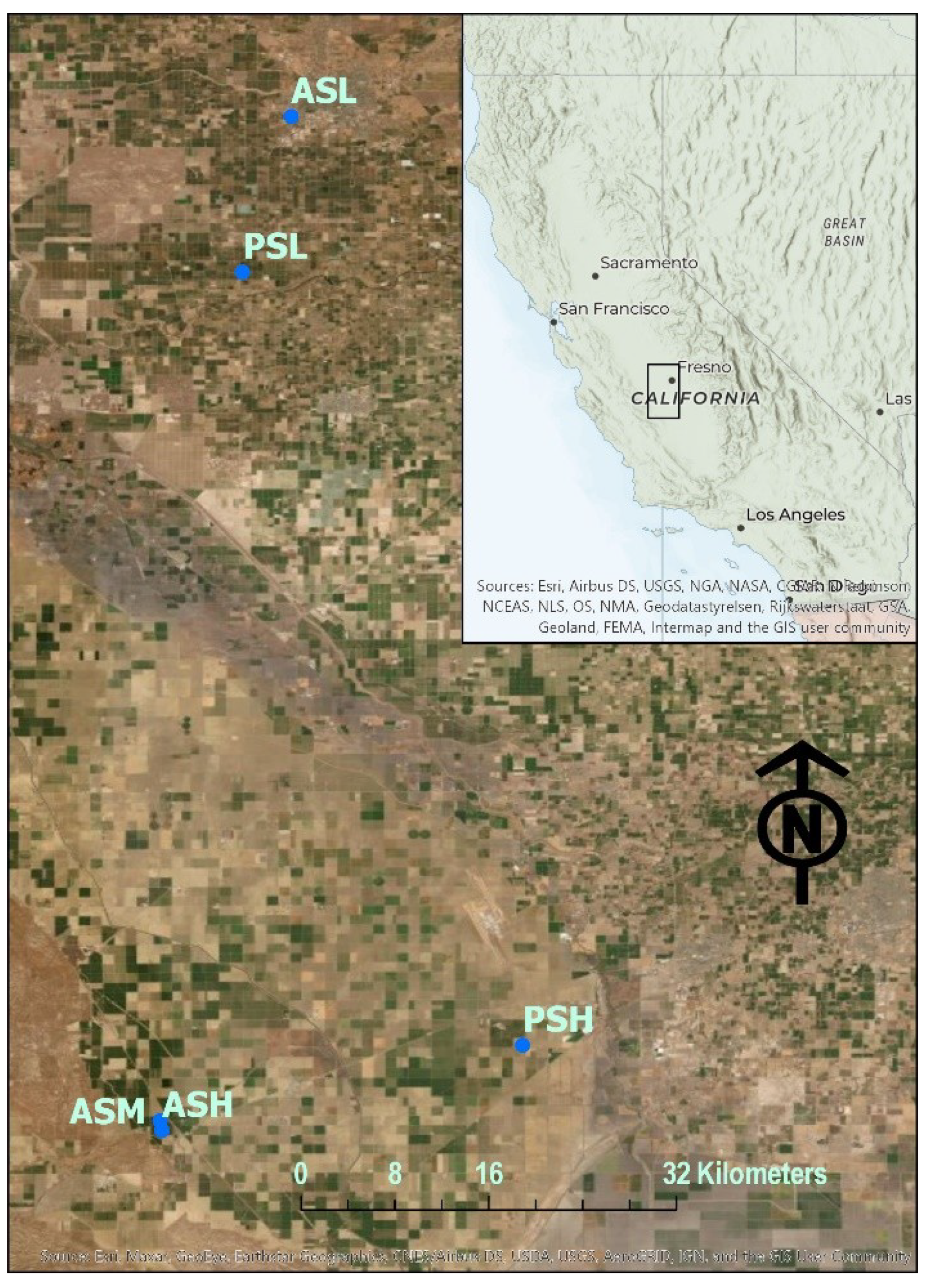
2.1. Field Sites

Five commercial SJV orchards were chosen for monitoring and evaluating seasonal water and salinity trends under drip irrigation. The network of field sites was part of a concurrent USDA-ARS study assessing soil and water quality impacts on crop productivity, with eddy covariance towers at all five orchards [14,15,16,17,18] (Figure 1 and Table 1—see also Fisher et al. [19]). The orchards had varying crop types (almond, pistachio), soil and water salinities (low, medium, high), and geographic locations (east vs. west SJV). The pistachio sites were of the Kerman (female)/Peters (male) cultivars with UCB-1 rootstock. ASL and ASH had three cultivars (Nonpareil, Monterey, and Mission) planted in alternating rows, while ASM had Butte and Padre cultivars. All almond sites had Nemaguard rootstock. In Table 1, the salinity designations low, medium, and high are informal descriptors indicating relative salinity levels at the sites. As a point of reference, USDA advises that salinity effects on crop yields are mostly negligible in the range ECe = 0–2 dS/m, can restrict the yields of sensitive crops in the range 2–4 dS/m, and will restrict the yields of most crops in the range 4–8 dS/m [20]. Almond is classified as a “sensitive” crop with reported Maas–Hoffman [21,22] threshold and slope parameters of 1.5 dS/m and 19% per dS/m, respectively [21]. Maas and Hoffman [21] rated pistachio as “moderately sensitive”, although subsequent studies found the threshold to be 8–10 dS/m and the slope around 10% per dS/m [23,24,25].
The five orchards were all irrigated with dual drip line systems (one line on either side of the tree line). As detailed below, the installation of monitoring equipment for the current study occurred during the fall of 2016. In wet water years, most SJV farmers have access to high-quality surface water for irrigation. The four years preceding the current study had been historically dry years [26]. During the drought, surface water deliveries were sharply curtailed for western SJV farmers. Many western SJV growers turned to groundwater for irrigation, which is frequently of lower quality (higher salinity) in the western SJV compared to less saline groundwater frequently found in the eastern SJV. For example, a recent USGS analysis found that the median total dissolved solids concentration for wells in the western SJV exceeded 1000 ppm (>1.5 dS/m) [27].
As our study started, our collaborators at the western sites believed their use of groundwater was beginning to salinize the soil and that the orchards were starting to show signs of distress, with one grower reporting a yield decline of more than 30%. However, a historically wet 2017 winter replenished much of the state’s water reservoirs, and surface water was generally available for irrigation during our study at all field sites except ASL, which uses high-quality groundwater exclusively. Signs of physiological stress at ASH (e.g., relatively greater prevalence of canker and tree mortality) persisted throughout the study period. Farmer-reported groundwater depths ranged from 52 m (~170 ft) at the eastern sites to over 240 m (~800 ft depth) in the west.

2.2. Soil Properties

Concurrent with the soil instrument installation locations, we collected soil samples for characterizing soil physical and chemical properties and root distributions. Samples were taken down to 1.2 m in 20 cm intervals for a total of 36 samples per orchard (3 pairs of sample holes along a drip line and in the middle of the row with six depth increments per sampling hole). Each of these individual samples provided bulk soil for chemical and root analysis. Soil textures were determined using an automated particle size analyzer (PARIO, METER Group, Pullman, Washington, DC, USA), which uses the integral suspension pressure method to analyze particle settling [28,29]. Bulk densities were determined from the oven-dry mass of undisturbed soil cores of known volume (6 Tempe cell samples per site concurrent with instrument installation—3 pairs of drip line and in the middle of the row samples gathered at the surface) [30]. The saturated hydraulic conductivity was measured for each depth interval using the constant head method on samples repacked to the field bulk densities [31]. Soluble cation concentrations of soil saturation extracts were determined by the ICP analysis. The electrical conductivity of the saturation paste extract (ECe) and pH were measured for collected soil samples using a conductivity/pH electrode calibrated against 0.01 M and 0.001 M KCl [32,33]. The cation exchange capacity (CEC) was determined using the ammonium acetate method [34]. Extracted cation solutions were analyzed for Ca, Mg, Na, and K. Roots were separated from the soil of each sample, and the mass of roots per sample was recorded. The measured roots were then used to construct normalized root density vs. depth curves for the sites.

2.3. Meteorological, Evapotranspiration, and Irrigation Data

Evapotranspiration in the orchards was measured using eddy covariance following the approach of Anderson et al. [35] and is described here briefly. Instrumentation included sonic anemometers, open-path infrared gas analyzers (IRGAs) for CO2 and H2O, four-component radiometers, and soil thermal heat flux plates. We grouped similar IRGAs by manufacturer, with EC150/IRGASON (Campbell Scientific, Logan, UT, USA) at PSL and PSH and 7500/7500A (Licor Inc., Lincoln, NE, USA) at ASL, ASM, and ASH. The high-frequency sonic anemometer and IRGA observations were processed to 30-min fluxes using EddyPro (v6.0; Licor, Inc. [36]). Gap filling [37,38] and energy budget closure of fluxes [39,40] were done following established approaches. Additional information about these sites can be found with their Ameriflux data descriptions [14,15,16,17,18]. The fetch for all sites was >200 m in all directions with the exception of the smaller ASL orchard, where the tower needed to be placed in the southeast corner of the orchard to maximize the fetch in the dominant prevailing wind direction (west-northwest). Fluxes at ASL where winds were from the east or southeast were gap-filled.
Modeled crop evapotranspiration (ETc) was estimated by multiplying monthly basal crop coefficients from the TOPS-SIMS satellite product [41] and reference evapotranspiration (ET0). Daily reference evapotranspiration (ET0) was available from nearby weather stations from the California Irrigation Management Information System (CIMIS) [42], and we used the closest stations to each of the orchards (Stations #15 Stratford for PSH, #80 Fresno State for PSL and ASL, and #205 Coalinga for ASH and ASM). We used the Penman–Monteith ET0 [43] instead of the default Pruitt–Doorenbos ET0 [44]. Tipping rain gauges were installed on the eddy covariance towers. Measured rain was compared with rain reported at nearby CIMIS weather stations, and the amounts were similar.
Irrigation water samples were collected periodically from drip lines during irrigation events when they coincided with field site visits; the sampling frequency thus varied considerably from site to site depending upon the frequency of irrigation. Collected irrigation water samples were analyzed for Ca, Mg, Na, and K using the ICP analysis. The irrigation water’s electrical conductivity and pH were measured with a conductivity/pH electrode. The number of samples at ASL was limited due to the higher-rate (and shorter duration) drip emitters that resulted in relatively few ongoing irrigation events when we were visiting the site for data collection and instrumentation maintenance. A record of irrigation depths vs. time for each site was constructed based on emitter discharge rates, the spatial density of emitters in the orchards, reports from growers on the timing and duration of irrigations, and our adjustment and augmentation of those reports based on a review of soil moisture time series data and tipping rain gauge data.

2.4. Soil Moisture, Salinity, and Statistical Analysis

The orchards were instrumented with frequency domain reflectometry sensors (GS3, METER Group Inc., Pullman, Washington, DC, USA), measuring bulk permittivity, temperature, and bulk electrical conductivity. Within each orchard, sensors were installed at three locations: a central “tower” location (so-called due to being co-located with an eddy covariance instrument tower) and two outlying locations referred to as “outer 1” and “outer 2”. The outer sensors were installed at approximately 75 m to the west-northwest and north-northwest directions from the tower within the larger tower footprint. At the tower locations, four sensors were installed directly beneath a dripline at 25, 50, 75, and 100 cm depths, and four sensors were installed midway between the dual drip lines (tree-line or mid-row between the two driplines) at 25, 50, 75, and 100 cm depths. Installations at the outer locations were at 50 and 100 cm in the mid-row position. Three sensors were installed at the 25, 75, and 100 cm depths at the drip position (5 total sensors).
Soil-specific calibrations for the GS3 sensors were developed according to “Method A” of METER [45,46,47]. Representative soil samples were collected from 25 cm at each site. In the lab, dry soil was mixed and packed in containers to the field bulk density, and a GS3 sensor was installed in the same manner as in the field. Water was added to the containers in steps. The soil container was weighed, and sensor readings were taken at each step. Soil volumetric water contents were calculated at each step from the soil dry bulk density and measured wet mass. The measurements of dielectric permittivity versus the soil volumetric water contents were plotted, and a quadratic calibration function for each site was fitted (r2 > 0.99 for all sites). Bulk electrical conductivity measured with the GS3 sensor was converted to pore-water electrical conductivity according to the Hilhorst method [48] as shown in Equation (1):
E C w   = ε p   . E C B ε b ε E C B = 0
where ECw is the pore-water electrical conductivity (dS/m), εp is the real portion of the dielectric permittivity of the soil pore water (unitless), ECB is the bulk electrical conductivity (dS/m) measured directly by the GS3 sensor, εb is the real portion of the dielectric permittivity of the bulk soil (unitless), and εECB = 0 is the real portion of the dielectric permittivity of the soil when bulk EC is 0 (unitless). As recommended by Hilhorst [48], we set εECB = 0 = 4.1. The real part of the permittivity εp was calculated from [METER, 2020a] following Equation (2):
ε P   = 80.3 0.37   ( T s o i l   20 )  
where Tsoil is the soil temperature (in degrees Celsius) measured by the GS3 sensor.
We used bootstrapping analysis (sampling with replacement) to assess the statistical significance of the micrometeorological and soil time-series data [49]. We assessed the sum of ET on a whole record and seasonal basis and the mean value for all other properties. For each variable, we ran 10,000 simulations to determine the 95% and 99% confidence intervals for each variable. Different variables were assessed as statistically significant or highly statistically significant if their 95% and 99% confidence intervals did not overlap.

3. Results

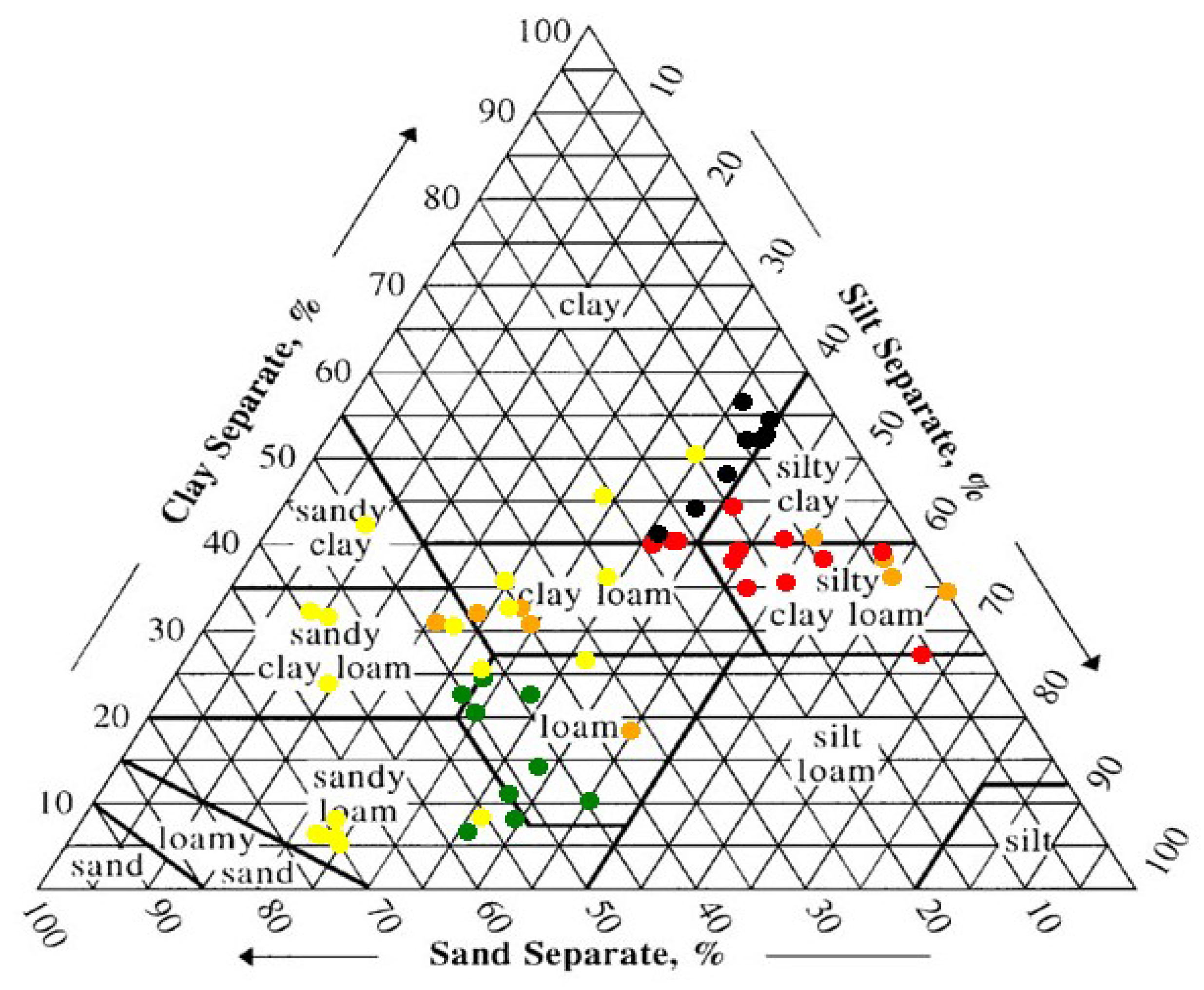
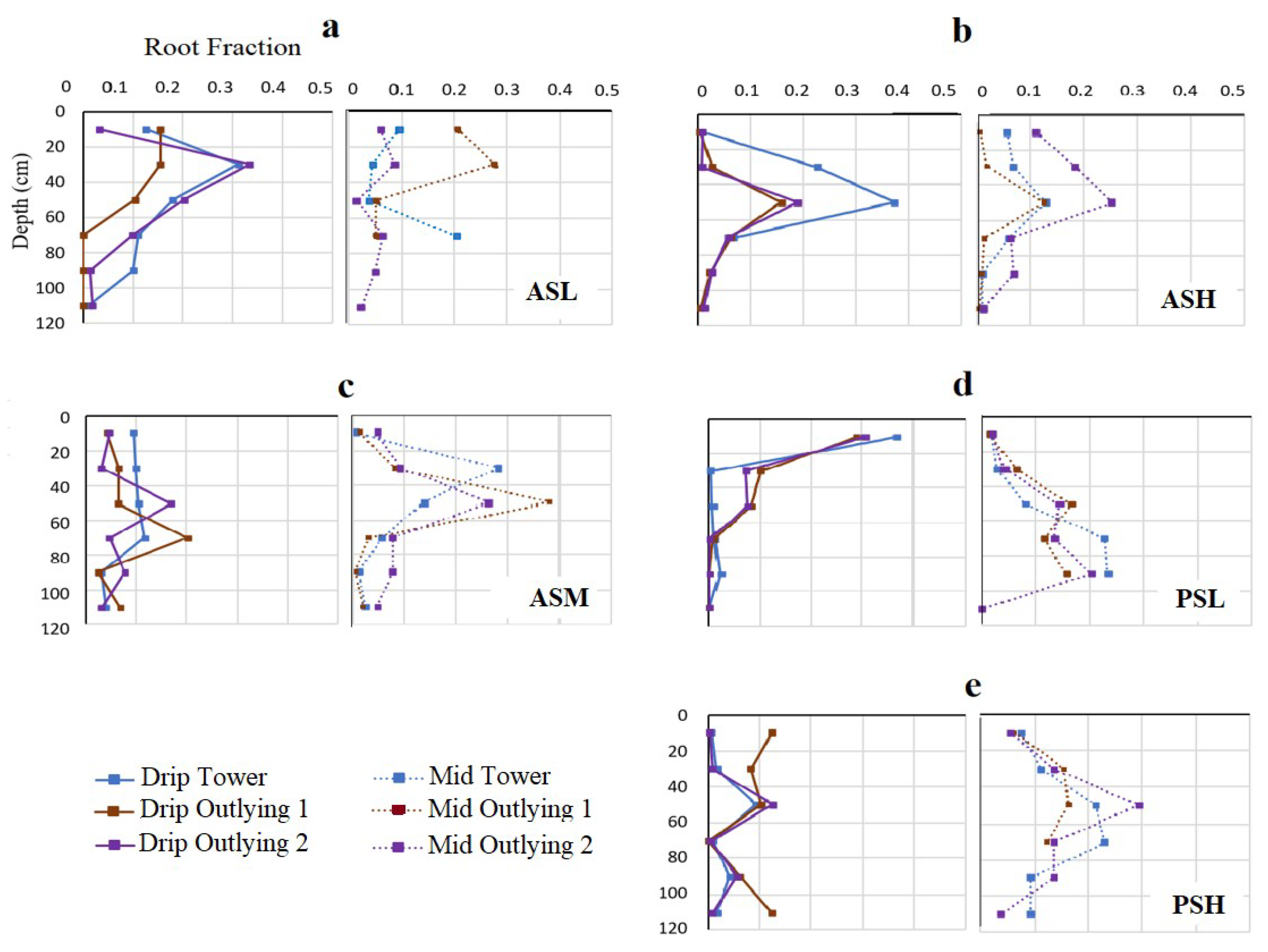
3.1. Soil Properties and Root Distribution

The measured soil characterization data are given in Appendix A (Table A1, Table A2, Table A3, Table A4 and Table A5). Figure 2 summarizes the soil textural properties of the five field sites. As expected from their geographic location, the eastern SJV sites generally have coarser textured soils than the western SJV sites. The p-values for statistical significance comparing the percent sand fractions of ASL and ASM were p = 0.017 and p < 1 × 10⁻⁵, respectively. The p-value for a sand fraction of PSL and PSH was less than 1 × 10⁻⁹. ASH and PSL had the largest variability, with soil samples encompassing five and six textural classes, respectively. The PSH samples were relatively homogeneous with a clay texture (Table A4). Samples from the ASM site had relatively high silt content (Table A2). The ASL site was also relatively uniform and mostly loam. Average hydraulic conductivity (Ksat) was lowest in the western SJV, with values of 6.8, 8.9, and 8.9 cm/day at ASM, ASH, and PSH, respectively. As expected, Ksat was significantly higher (p-value of 0.014 and p-value < 0.01 for PSL and ASL), with average values of 24.1 and 31.3 cm/day for ASL and PSL, respectively.

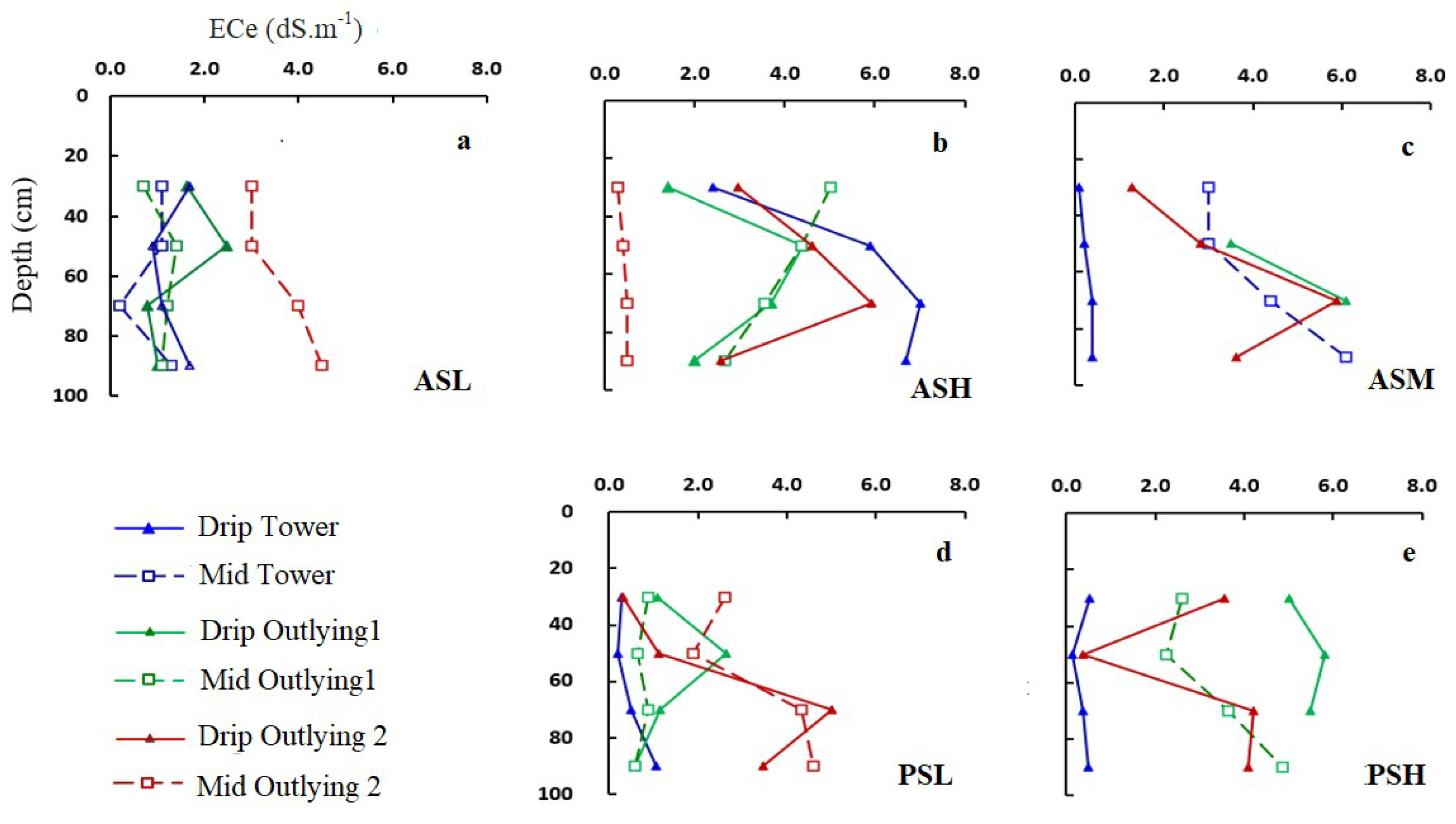
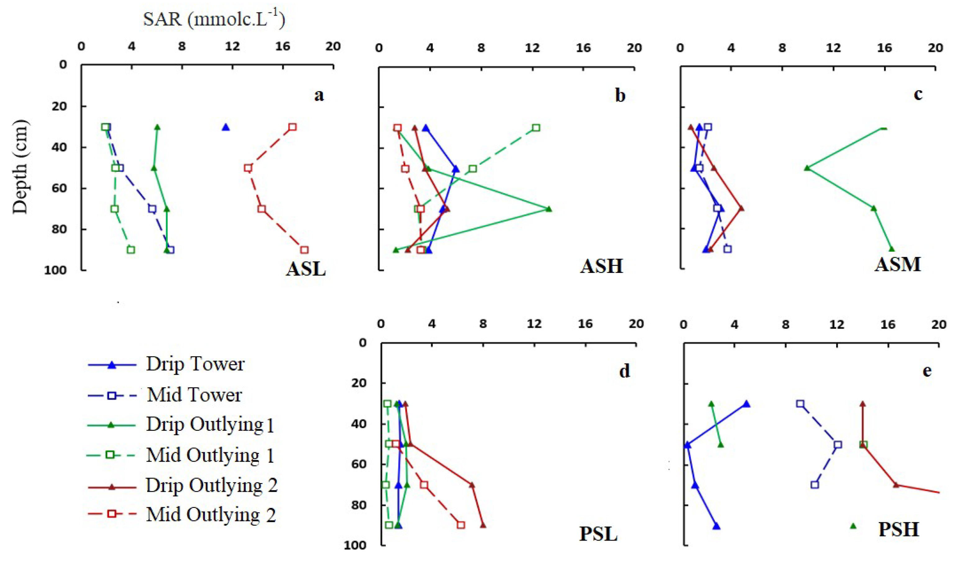
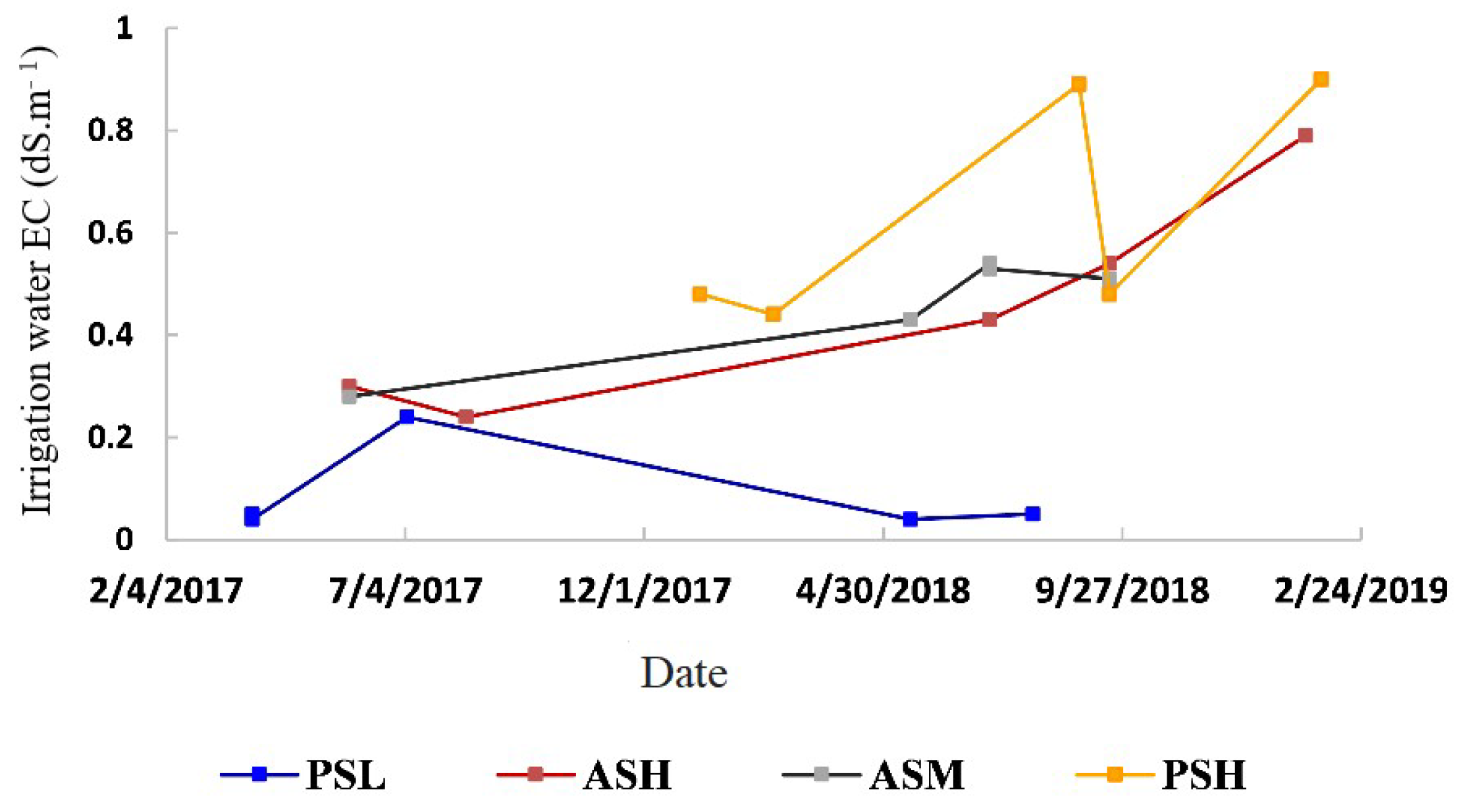
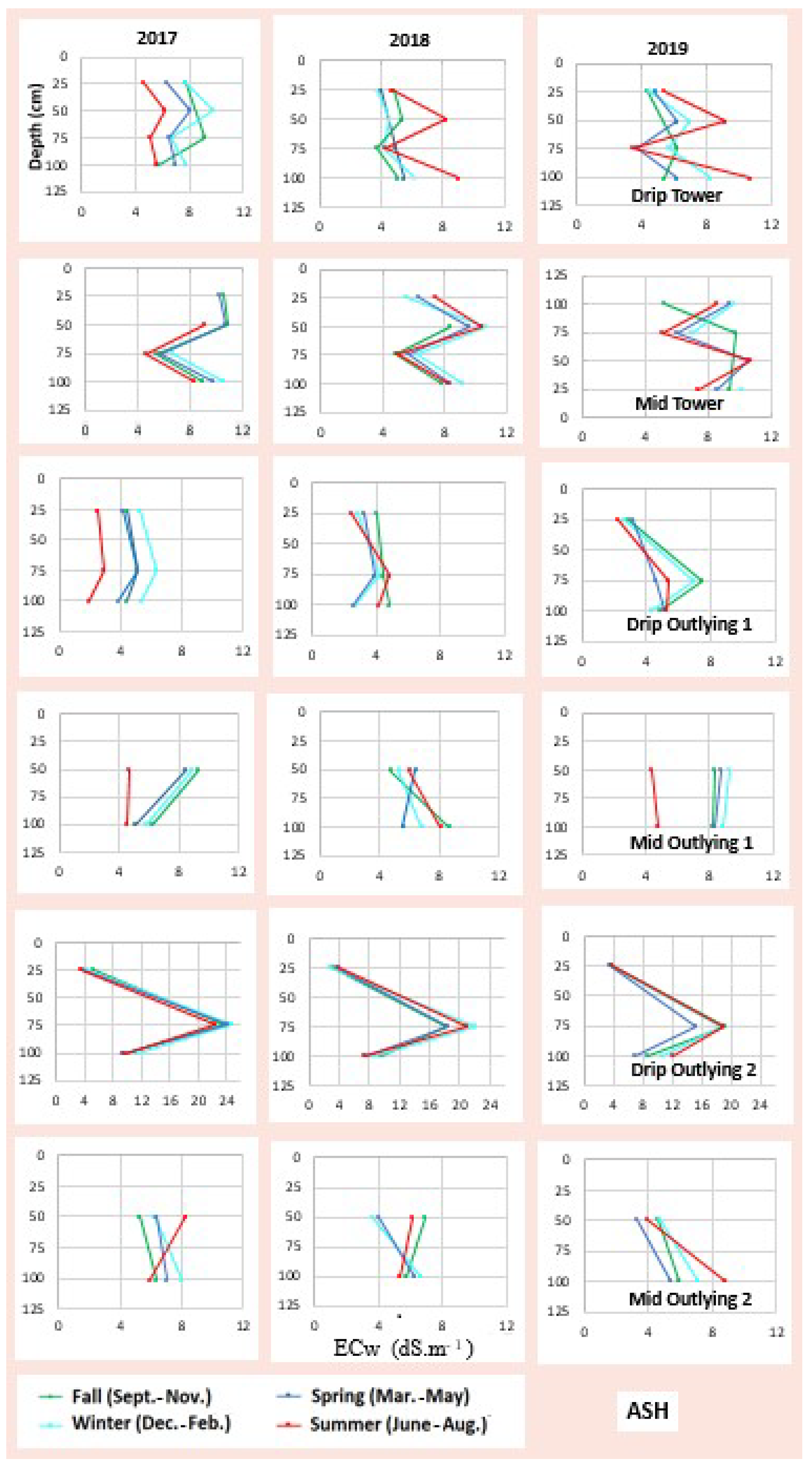
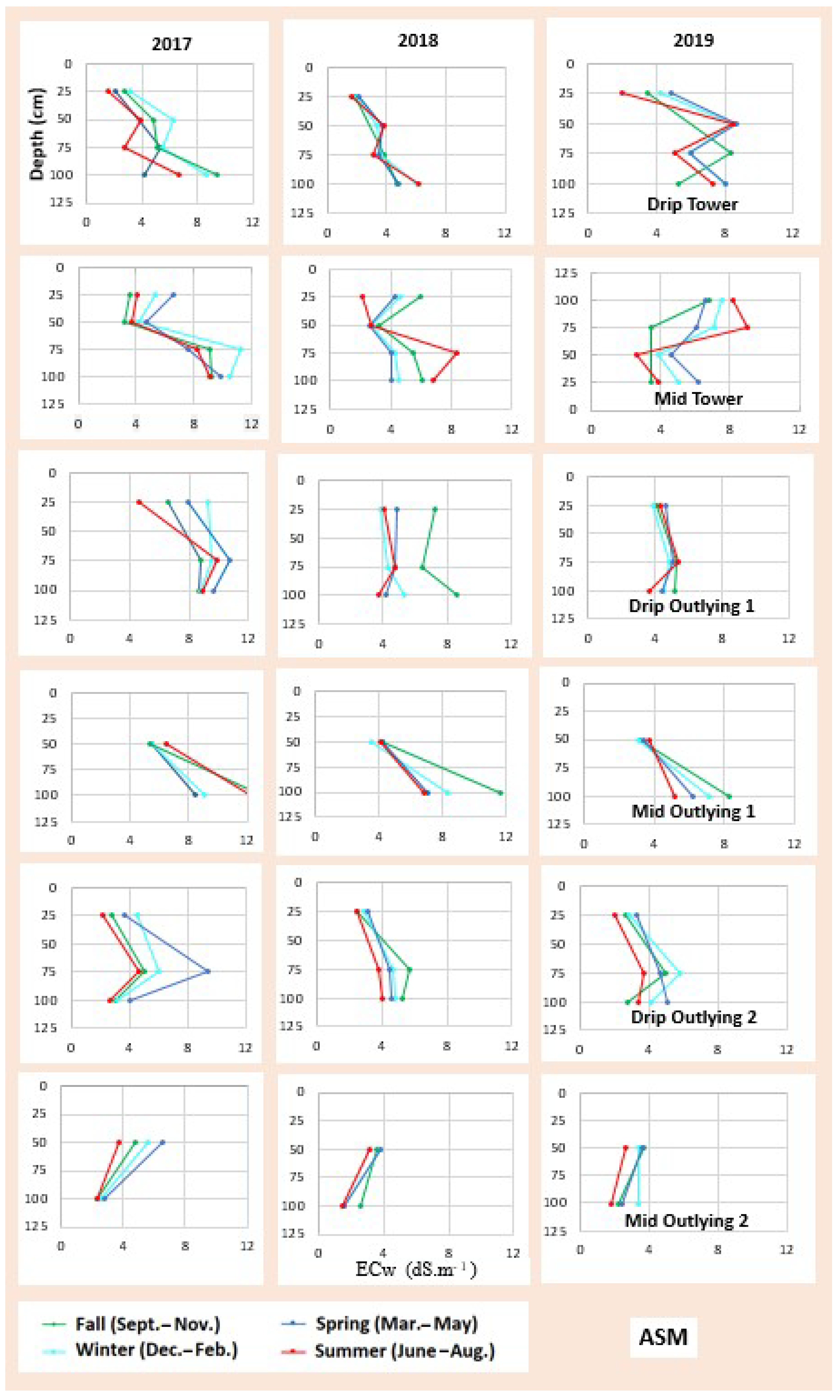
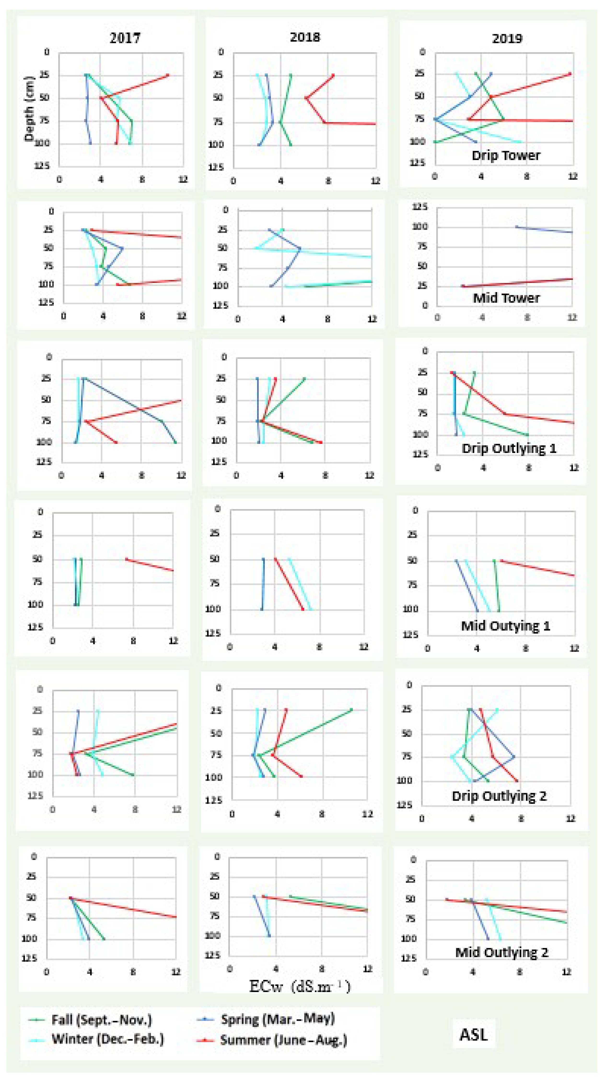
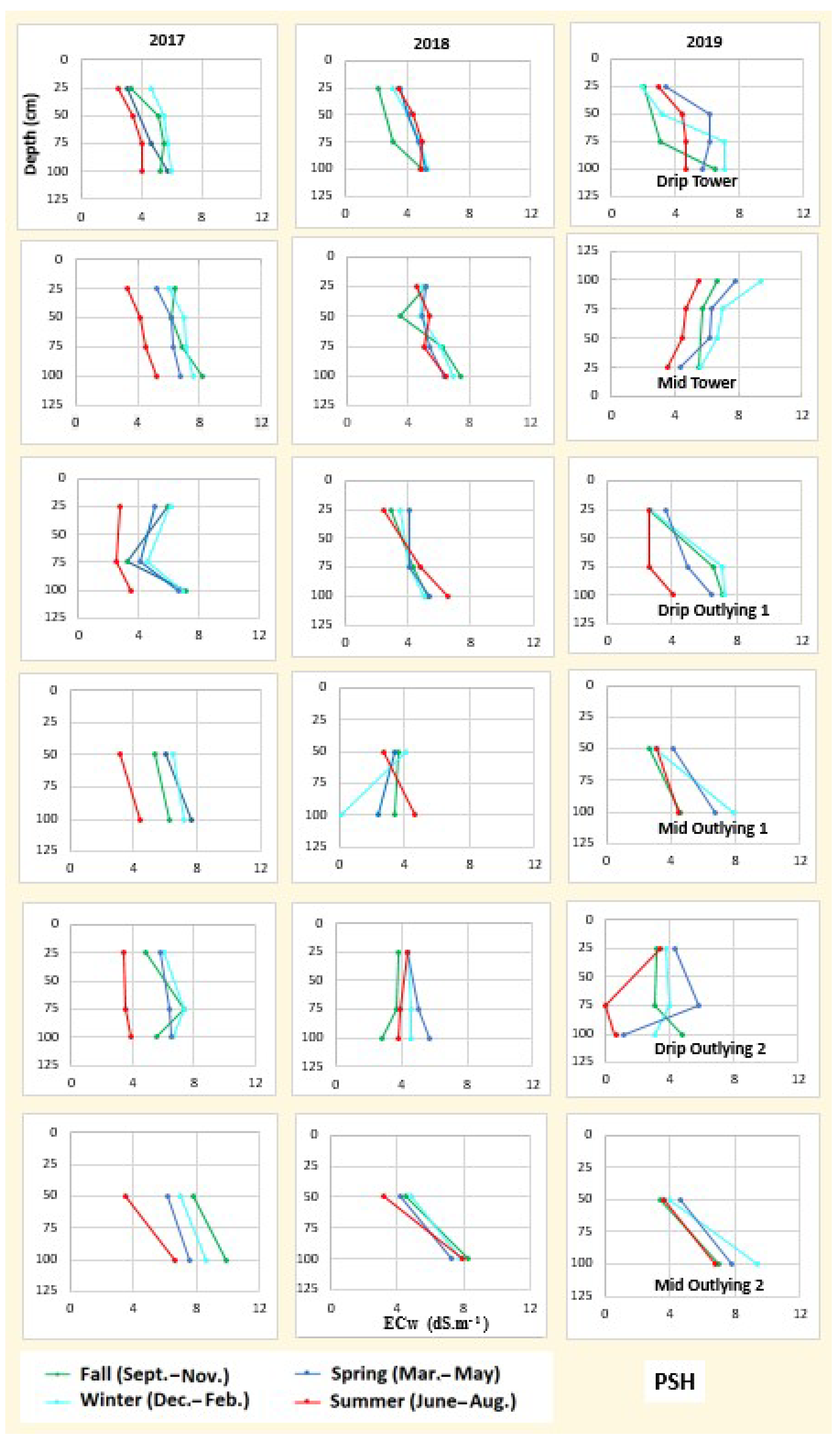
3.2. Soil Salinity and Root Distribution

The electrical conductivities (ECe) of saturation extracts for the soil samples collected during fall 2016 are shown in Figure 3. Corresponding sodium adsorption ratios (SARs) are shown in Figure 3. Initial soil salinity at the pistachio sites (Figure 3d,e) was below the reported pistachio threshold of 8–10 dS/m. Many of the salinity profiles measured in the almond fields had depth-averaged values that exceeded the reported threshold of 1.5 dS/m, particularly at the finer textured, western sites ASH and ASM (Figure 3a–c). At the ASH and ASM sites, salinity was highest and saturated hydraulic conductivity was lowest in the middle depths, 40–100 cm (Figure 3b,c; Table A2). ASL, ASM, and PSH all had locations where high sodium content in the soil profile suggests a possible sodicity hazard (Figure 4a,c,e). On average, eastern sites had significantly (p-value of 0.02 for ASL-ASH and p < 0.01 for PSL-PSH) lower sodium content (Table A7) than the western sites.
Figure 5 shows the observed root density profiles. The plotted values are the mass of the roots in a 20 cm soil sample (section of soil core) divided by the total mass found at each of the field sampling locations (i.e., the combined mass from the “drip” and “mid” excavations at each location within the field sites). For most of the sites and locations, most of the root mass was found between 20 and 60 cm. The eastern pistachio site PSL was an exception. Under the drip point at all three PSL locations, the peak root mass occurred within the 0–20 cm layer. Nevertheless, we found significant root biomass down to 100 cm under the midpoints. The coarse soil texture at the PSL site results in lower rates of lateral water spreading and, consequently, higher water availability and greater abundance of root mass at deeper locations beneath the mid-points. At the ASM and PSH sites, a relatively larger proportion of the root mass was found in the mid-point excavations than in the drip point excavations (Figure 5c,e).

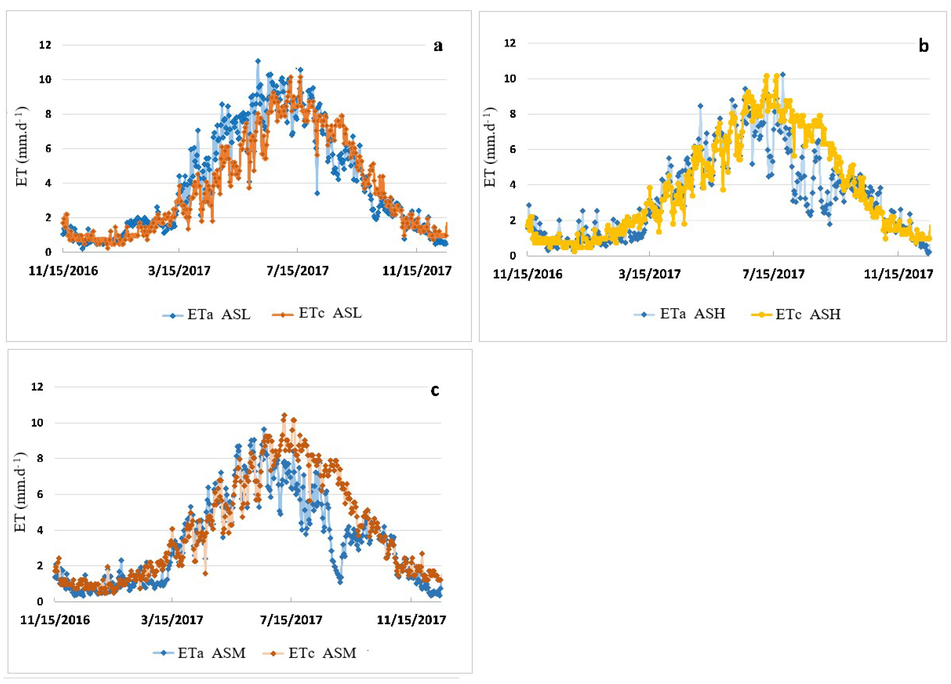
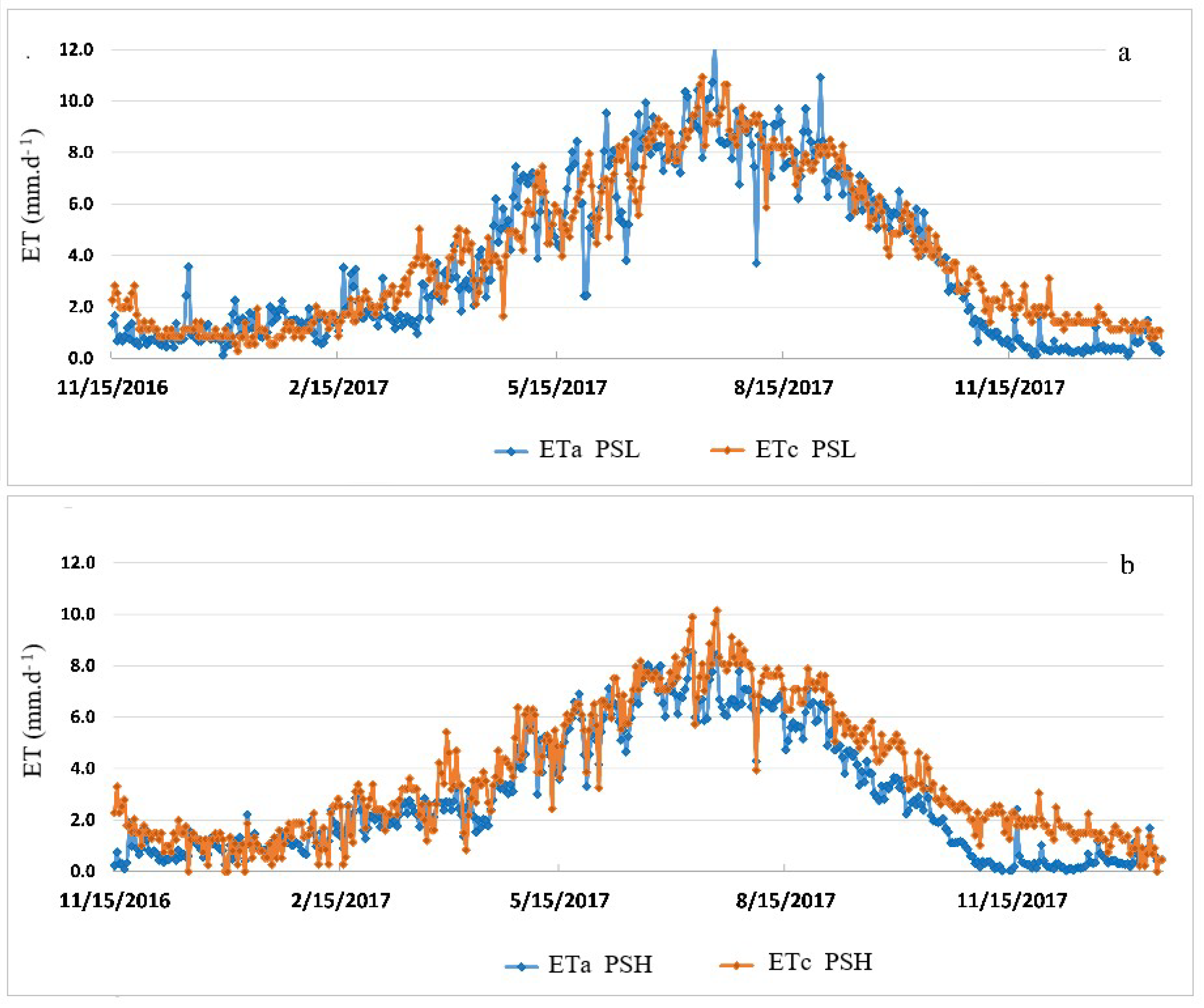
3.3. Evapotranspiration and Water Balances

The water years 2017 and 2019 were similar to one another, and both were wetter than the relatively dry 2018 water year (Table 2, Table 3, Table 4, Table 5 and Table 6). Irrigation water quality results are given in Figure 6 and Table A7. The eastern sites had irrigation waters with the lowest salinity, generally less than 0.1 dS/m. Samples from the western sites ranged approximately from 0.25 to 0.9 dS/m.
A detailed accounting of the seasonal water balances for the five sites across all seasons and years is given in Table 2, Table 3, Table 4, Table 5 and Table 6. Note that due to the start date of the current study, values provided for the first season, fall 2016, are only totals for two months rather than three. The apparent leaching fractions included in the tables were calculated as follows:
L F = 1 ( E T a ( I + P ) )
where I, P, and ETa are seasonal or annual totals of irrigation, precipitation, and measured ET, respectively. Thus, the leaching fraction (LF) calculations are based on an effective one-dimensional model of the soil and root zone, assuming water stored in the soil at the beginning of the season is the same as at the end as required by the steady-state assumption of the leaching fraction concept. Note that with this definition, LF will be negative if ETa > I + P. Negative values were observed in some summer seasons.
Measured evapotranspiration, ETa, matched modeled crop evapotranspiration, ETc, relatively well at the low salinity eastern sites ASL and PSL (data for the water year 2017 shown in Figure 7a and Figure 8a, respectively). However, at the western sites, ETa was highly significantly lower on an annual and multiannual basis for almonds, with some seasonal values also showing significance (Table 2 and Table 4; Figure 7b,c, respectively). Almond harvest took place in mid-August, which resulted in the largest discrepancies between ETa and ETc that are likely due to irrigation restrictions to encourage nut cracking and droppage for harvest. From the data, it is impossible to determine if the ET discrepancies at the western sites (Figure 7b,c and Figure 8b) were due to a relatively poor model for ETc estimates or if the western sites had reduced ET due to growth conditions being limited by higher soil and irrigation water salinities.
Eddy covariance data quality metrics ranged slightly for different sites. The percentage of gap-filled data ranged from 19 to 39% at ASH that required directional wind filling. PSL and PSH had gap filling of 31% and 32%, respectively, while ASM had 22%. ASM and ASL had the lowest gap-filling, likely due to higher nighttime winds at the adjacent sites. Daily energy balance closure ranged from 74 and 75% at PSH and PSL and was higher at the almond sites (87%, 85%, and 83% at ASH, ASM, and ASL, respectively).
The low salinity sites in the east were very consistent with respect to the ratio of measured annual evapotranspiration and calculated crop evapotranspiration. At the PSL eastern pistachio site, the ratio of measured and reference evapotranspiration, ETa/ETc, was 101%, 99%, and 104% for the water years 2017, 2018, and 2019, respectively (Table A6). The corresponding values for the ASL eastern almond site were 106%, 97%, and 99%. The overall three-year average for both sites was 101%.
The ETa/ETc ratios at the salt-affected western sites were notably lower on average, which is consistent with a lower canopy cover (as assessed through visual observations) and a statistically significantly higher ground heat flux (p < 0.01) and salinity stress. The ratios also exhibited greater interannual variability (Table 2, Table 3, Table 4, Table 5 and Table 6). The annual ET ratios at the western sites in 2017, 2018, and 2019 were 92%, 69%, and 101% at PSH; 79%, 92%, and 97% at ASM; and 79%, 90%, and 93% at ASH. The three-year average values were 87% at PSH, 90% at ASM, and 87% at ASH.
The apparent equivalent leaching fractions at the sites varied with year and season (Table 2, Table 3, Table 4, Table 5 and Table 6). PSL had the lowest range of annual leaching fractions, where the annual leaching fractions were 25%, 21%, and 17%, with a three-year average value of 21%. Other sites were more variable. For example, the ASL site had a similar average value of 19%, but with annual values of 29%, 0%, and 29%. Sites PSL (21%), ASL (19%), and ASH (18%) all had three-year averages near 20%, and the leaching fraction was not significantly different between sites of the same species. Site PSH had the highest annual leaching fraction at 27%, whereas ASM had the lowest at 11%.
Inter-seasonal variations in leaching were high (Table 2, Table 3, Table 4, Table 5 and Table 6). Winter is the rainy season, and a significant amount of leaching occurred, with apparent seasonal leaching fractions generally greater than or equal to 50%. Apparent leaching during the other seasons varied substantially, both across five field sites and year-to-year at individual sites.

3.4. Soil Water and Salinity

Seasonal root zone salinity profiles for 2017–2019 are shown for the five study sites in Figure A1, Figure A2, Figure A3, Figure A4 and Figure A5. Seasonal and annual trends are not easily identified from the plotted data. The plots in the top two rows of Figure A1, Figure A2, Figure A3, Figure A4 and Figure A5 are for the tower locations. Because they contain an extra monitoring depth, detailed interpretation and discussion of these plots are provided below.
Among the western field sites, ASH (Figure A1) and ASM (Figure A2) showed a general trend of increasing salinity between 2017 and 2019. Both sites relied on relatively saline irrigation water (Figure 6) and have medium-to-fine textured soils. The ASM site also had the lowest apparent average leaching fraction among the five sites at 11% (Table 3).
At the other western site, PSH, root zone salinity remained relatively constant during the three years. However, some higher salinity readings were obtained at the shallowest depths at the mid-tower position in 2019 (Figure A4). Site PSH had the highest average leaching fraction at 28% (Table 6). The western sites are in the rain shadow of the California Coast Ranges, and consequently, the eastern sites receive higher amounts of winter rains. The effect of winter rains at ASL and PSL can be seen in Figure A3 and Figure A5. The highest salinities are obtained in the summer (red curves) and then reduced between growing seasons by winter rain (blue curves).
One key question that can be addressed with in situ soil sensors is how frequently (and for how long) soil EC exceeds the Maas–Hoffman threshold [21]. While not exact, we can approximate extract EC (ECe) from pore-water EC (ECw) by relating the ECw and volumetric water content to saturated water content for the soil. When we evaluate this pseudo-ECe on a seasonal and long-term basis, a clearer divergence emerges between almonds and pistachios. At ASH and ASM, pseudo-ECe exceeds the Maas–Hoffman threshold for almonds (1.5 dS/m) for every season of this study. However, there were differing ranges of exceedance, with ASH exceeding 5 dS/m every quarter and reaching 7.4 dS/m in the fall/winter of the first year before substantial leaching water could be applied. Conversely, ASM was above the threshold but remained in the 2–4 dS/m range for the study period. PSH remained below the pistachio threshold of 8 dS/m (with the highest value of 7 dS/m in fall 2016), even though the site was above the “moderate” salinity threshold of Maas–Hoffman [21].

4. Discussion and Conclusions

As expected, the western sites had more significant salinity problems than the eastern sites. The western sites have finer textured soils and poorer quality irrigation water. Assuming the crop ET for the western sites was adequately modeled, the measured actual ET was about 90% of reference ET. While it is not possible to identify the cause of the ET reductions definitively from these observational data, it is plausible that salinity was a contributing factor. Two of the western sites showed some evidence of increasing soil salinity levels throughout the study. The third western site appeared to maintain the same salinity level by imposing a relatively high apparent leaching fraction (28%). Across the three western sites, the annual average apparent leaching fraction ranged from 11 to 28%. Evidence of restricted water flow at deeper soil layers was evident at ASH, with some samples having low saturated hydraulic conductivity (<2 cm/day). The highest leaching fraction at ASH, combined with that orchard’s use of gypsum for salinity control, likely explains the similarly high initial EC profiles at ASH and PSH, but the lower SAR at ASH compared to PSH.
In contrast to the western sites, overall salinity was controlled at the eastern sites, and crop ET appeared maximal, with measured ET matching modeled ET almost exactly each year (crop coefficients of ~1 for both PSL and ASL). Apparent leaching fractions at the eastern sites were approximately 20%. The lack of any evidence of salinity issues at PSL and ASL indicate that carefully selected orchards in the eastern SJV can serve as suitable controls for salinity comparisons with salt-affected fields in the western SJV.
Reductions in crop ET with salinity stress are often modeled as being proportional to the yield reductions due to salinity. For example, the Maas–Hoffman threshold and slope parameters are explicitly incorporated into the FAO-56 model for calculating crop ET [43]. Based on the high soil electrical conductivities observed at ASH (Figure A1), we would expect substantial decreases in ET due to the exceedance of the Maas–Hoffman threshold for almonds. However, while there are some declines in ET at ASH compared to ASL, they do not track the Maas–Hoffman parameters for almonds. Sanden et al. [50] found similarly higher salinity tolerance for almond orchards in the western SJV, with no significant yield decreases up to the maximum observed ECe of ~4 dS/m. The results from both Sanden et al. [50] and this study suggest that current commercial cultivars may have a higher salinity tolerance than previously assumed for almonds. Further work is needed to understand how irrigation management, cultivation practices, and new cultivars may increase almond salinity tolerance.
One possible approach to re-evaluate Maas–Hoffman parameters for almonds would be to conduct regional scale analyses. These could include relating yield to larger scale salinity maps such as those produced by Scudiero et al. [51], which would help further determine whether the Maas–Hoffman threshold and slope are overly conservative. In the absence of yield data, an analysis of regional ET for orchards in the SJV compared against salinity maps [51] could help assess salinity impacts on crop productivity
Another approach for understanding the mechanisms of salinity movement in the soil and their impact on soil water and solute balances is applying a process-based model. In the accompanying manuscript (part 2), we present the results of a one-dimensional model (HYDRUS 1-D) in helping us to understand the seasonal and interannual salinity dynamics across a natural salinity gradient.

Author Contributions

Conceptualization, S.A.H., R.G.A., T.H.S. and J.Š.; Data curation, R.G.A.; Formal analysis, S.A.H.; Funding acquisition, S.A.H. and J.Š.; Methodology, S.A.H., R.G.A., T.H.S. and J.Š.; Resources, S.A.H., R.G.A., T.H.S., G.D.J., D.W. and J.Š.; Software, J.Š.; Writing—original draft, S.A.H., R.G.A., T.H.S. and J.Š.; Writing—review & editing, S.A.H., R.G.A., T.H.S., G.D.J., D.W. and J.Š. All authors have read and agreed to the published version of the manuscript.

Funding

S.A.H was in part by an international Ph.D. fellowship from the Cultural and Education section, Egyptian Higher Education Ministry, Egypt, and by a graduate student research fellowship from the Department of Environmental Sciences, University of California, Riverside. Field data collection was funded by the USDA-ARS Office of National Programs projects 2036-61000-018-00-D (R.G.A. and T.H.S.) and 2034-13000-012-00-D (D.W.). J.S. was funded by the USDA National Institutes of Food and Agriculture Multistate Project W4188 (Project No. 1021006 CA-R-ENS-5047-RR).

Institutional Review Board Statement

Not applicable.

Informed Consent Statement

Not applicable.

Data Availability Statement

Eddy covariance data are available via Ameriflux. Other data are available upon reasonable request to the corresponding authors.

Acknowledgments

The authors would like to thank Dennise Jenkins, Towfiq Khan, and Kailuh Menefee (USDA-ARS) for their assistance with field and laboratory work. We also thank Professors Laosheng Wu and Robert Graham (University of California, Riverside) and their laboratories for assistance with soil and water sample analysis. Mention of trade names or commercial products in this publication is solely for the purpose of providing specific information and does not imply recommendation or endorsement by the U.S. Department of Agriculture. The U.S. Department of Agriculture prohibits discrimination in all its programs and activities on the basis of race, color, national origin, age, disability, and where applicable, sex, marital status, familial status, parental status, religion, sexual orientation, genetic information, political beliefs, reprisal, or because all or part of an individual’s income is derived from any public assistance program. (Not all prohibited bases apply to all programs.) Persons with disabilities who require alternative means for communication of program information (Braille, large print, audiotape, etc.) should contact USDA’s TARGET Center at (202) 720-2600 (voice and TDD). To file a complaint of discrimination, write to USDA, Director, Office of Civil Rights, 1400 Independence Avenue, S.W., Washington, D.C. 20250-9410, or call (800) 795-3272 (voice) or (202) 720-6382 (TDD). USDA is an equal opportunity provider and employer.

Conflicts of Interest

The authors declare no conflict of interest.

Appendix A

Figure A1. Seasonal average root zone soil water EC at six monitoring locations at the western almond site ASH.
Soilsystems 05 00050 g0a1
Figure A2. Seasonal average root zone soil water EC at six monitoring locations at the western almond site ASM.
Soilsystems 05 00050 g0a2
Figure A3. Seasonal average root zone soil water EC at six monitoring locations at the eastern almond site ASL.
Soilsystems 05 00050 g0a3
Figure A4. Seasonal average root zone soil water EC at six monitoring locations at the western pistachio site PSH.
Soilsystems 05 00050 g0a4
Figure A5. Seasonal average root zone soil water EC at six monitoring locations at the eastern pistachio site PSL.
Soilsystems 05 00050 g0a5
Table A1. Measured soil properties of the ASH site.
LocationPositionDepthCECExchangeable Sodium PercentageSodium Adsorption RatioECepHSandSiltClaySaturated Hydraulic Conductivity
cmmmolc/kg%(mmolc/L)0.5dS/m %%%cm d−1
TowerDrip0–20 49.520.130.4
20–4062.5722.153.62.46.740.928.930.216.15
40–60130.6434.796.05.98.0 5.62
60–80151.4732.025.07.08.05.259.235.60.5
100–120138.1333.243.86.78.04.957.337.82.05
Mid0–20
20–407.7922.40
40–608.5116.32
60–8056.411.21
100–12047.711.47
Outlying 1Drip0–20
20–40 1.331.46.6
40–60 3.864.48.1
60–80 13.313.78.21.065.034.0
100–120 1.342.07.8
Mid0–20
20–40 12.35.07.9
40–60 7.34.48.1
60–80 3.13.68.1
100–120 3.42.77.7
Outlying 2Drip0–20 45.223.431.4
20–4063.2423.882.83.08.440.827.032.210.83
40–60112.1421.973.64.68.5 6.33
60–80134.4322.725.35.98.410.249.640.22.87
100–12078.3022.602.32.68.238.044.217.826.59
Mid0–20
20–4073.4322.361.50.38.1
40–60109.5020.442.0--
60–80113.1722.503.20.58.3
100–12099.9427.343.30.5
Table A2. Measured soil properties of the ASM site.
LocationPositionDepthCECExchangeable Sodium PercentageSodium Adsorption RatioECepHSandSiltClaySaturated Hydraulic Conductivity
cmmmolc/kg%(mmolc/L)0.5dS·m−1 %%%cm/d−1
TowerDrip0–20 18.843.637.69.37
20–40124.495.171.51.38.517.743.538.83.38
40–6075.786.461.12.28.6
60–80133.113.873.24.58.24.656.838.61.01
100–120115.224.952.03.98.27.066.426.68.72
Mid0–20
20–40 2.13.08.3
40–60 1.53.08.1
60–80 2.94.48.3
100–120 3.76.18.1
Outlying 1Drip0–20
20–40100.2815.0516.0 15.740.543.8
40–60125.3416.969.93.58.122.737.539.8
60–80128.8220.1915.16.18.4
80–100 15.349.735.0
100–120 16.6 13.047.040.0
Outlying 2Drip0–20 25.235.439.45.77
20–40 0.91.37.923.237.039.82.27
60–80 2.62.88.6
80–100 4.85.98.219.146.534.47.48
100–120 2.43.68.210.551.737.816.71
Table A3. Measured soil properties of the ASL site.
LocationPositionDepthCECExchangeable Sodium
Percentage
Sodium
Adsorption Ratio
ECepHSandSiltClaySaturated Hydraulic Conductivity
cmmmolc/kg%(mmolc/L)0.5dS/m %%%cm d−1
TowerDrip20–4044.5915.39 1.78.152.736.710.629.18
40–6048.1916.80 0.98.248.537.913.617.74
60–8068.6115.62 1.17.353.738.77.621.82
100–12078.0115.68 1.78.158.635.26.227.78
Mid20–4035.7510.872.01.18.2
40–6038.8513.453.11.1
60–8046.2615.545.60.28.7
100–12086.5313.397.01.38.6
Outlying 1Drip20–4035.1422.906.01.68.645.033.022.0
40–6034.3817.735.72.58.348.327.724.0
60–8031.3717.096.80.8 51.326.722.0
100–12029.7223.906.81.08.351.029.020.0
Mid20–4033.9010.611.90.77.5
40–6030.3613.212.71.47.9
60–8032.6010.822.61.28.2
100–12033.0116.604.01.17.6
20–40 16.83.08.9
40–60 13.33.08.8
60–80 14.34.08.2
100–120 17.74.58.5
Table A4. Measured soil properties of the PSH site.
LocationPositionDepthCECExchangeable Sodium PercentageSodium Adsorption RatioECepHSandSiltClaySaturated Hydraulic Conductivity
cmmmolc/kg%(mmolc/L)0.5dS/m %%%cm d−1
TowerDrip0–20 10.537.951.6
20–4097.0721.050.347.58.539.352.221.85
40–60120.6420.580.91.58.514.338.147.67.03
60–8096.4319.232.93.77.5 7.02
100–120 2.64.8 24.235.240.613.57
Mid0–20
20–40
40–60
100–120
Outlying 1Drip0–20
20–40126.5310.302.165.07.89.239.251.6
40–60119.5910.212.895.87.87.338.953.8
60–80129.588.04 8.735.455.9
100–12053.0712.1313.325.57.419.137.243.7
Mid0–20
20–40103.4211.23 2.67.3
40–60106.4410.1214.12.37.4
60–80118.368.01 3.77.2
100–120106.345.73 4.97.0
Outlying 2Drip0–20
20–40117.7621.4314.033.68.3 8.90
60–80124.5323.2014.053.88.4 3.79
100–120166.8225.5934.48 9.79
Table A5. Measured soil properties of the PSL site.
LocationPositionDepthCECExchangeable Sodium PercentageSodium Adsorption RatioECepHSandSiltClaySaturated
Hydraulic Conductivity
cmmmolc/kg%(mmolc/L)0.5dS/m %%%cm d−1
TowerDrip0–20 72.421.95.7
20–406.0816.251.420.37.672.621.45.950.95
40–608.107.961.470.26.970.022.57.530.33
60–809.9014.441.390.56.671.124.24.713.81
100–12030.4611.501.331.17.956.735.67.711.20
Outlying 1Drip0–20
20–40 1.21.17.963.013.823.2
40–60 2.02.68.059.010.031.0
60–80 2.01.17.960.38.031.7
100–120 1.30.6 50.28.041.8
Mid0–20
20–40 0.50.98.4
40–60 0.60.78.2
60–80 0.30.98.2
100–120 0.60.67.8
Outlying 2Drip0–20
20–406.1226.271.90.36.342.026.032.0
40–608.0316.072.31.16.938.036.026.0
60–8054.881.317.15.07.248.022.030.0
100–12047.841.518.03.38.431.333.035.7
Mid0–20
20–408.5711.021.22.67.148.027.025.0
40–6021.4015.593.41.98.216.034.050.0
60–8082.2516.716.34.37.627.028.045.0
100–12047.8316.634.94.38.440.724.035.3
Table A6. Shallow (0–20 cm) soil concentrations for select elements.
ClNaCaKMgBMo
meq/Lmeq/Lmeq/Lmeq/Lmeq/Lppmppm
ASL2.152.385.040.282.420.082.42
ASM0.4812.2620.821.0011.400.1711.40
ASH1.0411.9814.770.777.021.177.02
PSL0.281.282.680.831.380.281.38
PSH1.1019.2017.380.646.532.606.53
Bolded values for PSH, ASM, or ASH values represents values that are significantly (p < 0.05) different than PSL or ASL.
Table A7. Irrigation water salinity, sodicity, and ionic composition.
SitesDay of IrrigationECiw
(dS/m)
SAR
(mmolc/L )0.5
pHCa2+
(mmolc/L)
Mg2+
(mmolc/L)
Na+
(mmolc/L)
K+
(mmolc.l/L)
1ASH30 May 20170.3 7.780.320.321.290.17
11 Aug 20170.241.47.140.350.351.540.09
6 Jul 20180.43 7.61.040.512.240.1
19 Sep 20180.54 6.950.310.291.090.07
20 Jan 20190.79 7.81.11.164.760.19
2ASM30 May 20170.281.77.70.330.331.470.08
17 May 20180.43 7.690.870.582.470.13
6 Jul 20180.541.87.720.430.613.260.12
19 Sep 20180.51 7.890.460.522.310.11
5 Jan 20190.48 7.80.910.695.980.14
3PSL30 Mar 20170.050.487.640.10.020.190.05
5 Jul 20170.24 7.80.490.241.150.07
17 May 20180.04 7.20.080.020.190.04
2 Aug 20180.05 8.060.070.010.150.04
4PSH20 Feb 20180.44 7.570.520.592.860.16
31 Aug 20180.894.17.720.510.562.540.12
19 Sep 20180.4837.930.440.573.030.11
30 Jan 20190.9 7.771.220.745.890.09

References

  1. Schoups, G.; Hopmans, J.W.; Young, C.A.; Vrugt, J.A.; Wallender, W.W.; Tanji, K.K.; Panday, S. Sustainability of Irrigated Agriculture in the San Joaquin Valley, California. Proc. Natl. Acad. Sci. USA 2005, 102, 15352–15356. [Google Scholar] [CrossRef] [Green Version]
  2. Tindula, G.N.; Orang, M.N.; Snyder, R.L. Survey of Irrigation Methods in California in 2010. J. Irrig. Drain. Eng. 2013, 139, 233–238. [Google Scholar] [CrossRef]
  3. Hanson, B.; May, D. Drip Irrigation Salinity Management for Row Crops; University of California, Agriculture and Natural Resources: Davis, CA, USA, 2011; ISBN 978-1-60107-740-0. [Google Scholar]
  4. Machado, R.M.; Serralheiro, R.P. Soil Salinity: Effect on Vegetable Crop Growth. Management Practices to Prevent and Mitigate Soil Salinization. Horticulturae 2017, 3, 30. [Google Scholar] [CrossRef]
  5. Kelsey, R.; Hart, A.; Butterfield, H.S.; Vink, D. Groundwater Sustainability in the San Joaquin Valley: Multiple Benefits If Agricultural Lands Are Retired and Restored Strategically. Calif. Agric. 2018, 72, 151–154. [Google Scholar] [CrossRef] [Green Version]
  6. Galloway, D.L.; Jones, D.R.; Ingebritsen, S.E. Land Subsidence in the United States; Circular 1182; US Geological Surwey: Denver, CO, USA, 1999. [Google Scholar]
  7. Carle, D. Introduction to Water in California, 2nd ed.; University of California Press: Oakland, CA, USA, 2016; ISBN 978-0-520-28789-1. [Google Scholar]
  8. Quinn, N.W.T. The San Joaquin Valley: Salinity and Drainage Problems and the Framework for a Response. In Salinity and Drainage in San Joaquin Valley, California: Science, Technology, and Policy; Chang, A.C., Brawer Silva, D., Eds.; Springer: Dordrecht, The Netherlands, 2014; pp. 47–97. ISBN 978-94-007-6851-2. [Google Scholar]
  9. Quinn, N.W.T.; Delamore, M.L. Issues of Sustainable Irrigated Agriculture in the San Joaquin Valley of California in a Changing Regulatory Environment Concerning Water Quality and Protection of Wildlife; Lawrence Berkeley National Laboratory: Berkelye, CA, USA, 1994. [Google Scholar]
  10. He, R.; Jin, Y.; Kandelous, M.M.; Zaccaria, D.; Sanden, B.L.; Snyder, R.L.; Jiang, J.; Hopmans, J.W. Evapotranspiration Estimate over an Almond Orchard Using Landsat Satellite Observations. Remote Sens. 2017, 9, 436. [Google Scholar] [CrossRef] [Green Version]
  11. Gaines, R.W. Central Valley Project Water Development: Historical Background, Economic Impacts, and Future Outlook; R.W. Gaines: Roseville, CA, USA, 1986. [Google Scholar]
  12. Department of Water Resources. Drainage Management in the San Joaquin Valley, a Status Report; Department of Water Resources: Sacramento, CA, USA, 1998.
  13. Bellvert, J.; Adeline, K.; Baram, S.; Pierce, L.; Sanden, B.L.; Smart, D.R. Monitoring Crop Evapotranspiration and Crop Coefficients Over an Almond and Pistachio Orchard Throughout Remote Sensing. Remote Sens. 2018, 10, 2001. [Google Scholar] [CrossRef] [Green Version]
  14. Anderson, R. AmeriFlux US-PSL USSL San Joaquin Valley Pistachio Low; US Department of Energy, Office of Biological and Environmental Research: Berkeley, CA, USA, 2020.
  15. Anderson, R. AmeriFlux US-PSH USSL San Joaquin Valley Pistachio High; USDA-ARS: US Department of Energy, Office of Biological and Environmental Research: Berkeley, CA, USA, 2020. [Google Scholar]
  16. Anderson, R. AmeriFlux US-ASL USSL San Joaquin Valley Almond Low Salinity; US Department of Energy, Office of Biological and Environmental Research: Berkeley, CA, USA, 2020.
  17. Anderson, R. AmeriFlux US-ASM USSL San Joaquin Valley Almond Medium Salinity; US Department of Energy, Office of Biological and Environmental Research: Berkeley, CA, USA, 2020.
  18. Anderson, R. AmeriFlux US-ASH USSL San Joaquin Valley Almond High Salinity; US Department of Energy, Office of Biological and Environmental Research: Berkeley, CA, USA, 2020.
  19. Fisher, J.B.; Lee, B.; Purdy, A.J.; Halverson, G.H.; Dohlen, M.B.; Cawse-Nicholson, K.; Wang, A.; Anderson, R.G.; Aragon, B.; Arain, M.A.; et al. ECOSTRESS: NASA’s Next Generation Mission to Measure Evapotranspiration From the International Space Station. Water Resour. Res. 2020, 56, e2019WR026058. [Google Scholar] [CrossRef]
  20. US Salinity Laboratory. Diagnosis and Improvement of Saline and Alkali Soils; Richards, L.A., Ed.; Handbook; Soil and Water Conservative Research Branch, Agricultural Research Service, US Department of Agriculture: Washington, DC, USA, 1954.
  21. Maas, E.V.; Hoffman, G. Crop Salt Tolerance-Current Assessment. J. Irrig. Drain. Div. ASCE 1977, 103, 115–134. [Google Scholar] [CrossRef]
  22. van Straten, G.; de Vos, A.C.; Rozema, J.; Bruning, B.; van Bodegom, P.M. An Improved Methodology to Evaluate Crop Salt Tolerance from Field Trials. Agric. Water Manag. 2019, 213, 375–387. [Google Scholar] [CrossRef]
  23. Sanden, B.L.; Ferguson, L.; Corwin, D.L. Development and Long-Term Salt Tolerance of Pistachios from Planting to Maturity Using Saline Groundwater. Acta Hortic. 2014, 1028, 327–332. [Google Scholar] [CrossRef]
  24. Sepaskhah, A.R.; Maftoun, M. Relative Salt Tolerance of Pistachio Cultivars. J. Hortic. Sci. 1988, 63, 157–162. [Google Scholar] [CrossRef]
  25. Ferguson, L.; Poss, J.A.; Grattan, S.M.; Grieve, C.M.; Wang, D.; Wilson, C.; Donavan, T.A.; Chao, C.T. Pistachio Rootstocks Influence Scion Growth and Ion Relations under Salinity and Boron Stress. J. Am. Soc. Hortic. Sci. JASHS 2002, 127, 194–199. [Google Scholar] [CrossRef] [Green Version]
  26. Griffin, D.; Anchukaitis, K.J. How Unusual Is the 2012–2014 California Drought? Geophys. Res. Lett. 2014, 41, 9017–9023. [Google Scholar] [CrossRef] [Green Version]
  27. Fram, M.S. Groundwater Quality in the Western San Joaquin Valley Study Unit, 2010: California GAMA Priority Basin Project; Scientific Investigations Report; U.S. Geological Survey: Reston, VA, USA, 2017; p. 146. [Google Scholar]
  28. Gee, G.W.; Or, D. 2.4 Particle-Size Analysis. In Methods of Soil Analysis; John Wiley & Sons, Ltd.: Hoboken, NJ, USA, 2002; pp. 255–293. ISBN 978-0-89118-893-3. [Google Scholar]
  29. Durner, W.; Iden, S.C.; von Unold, G. The Integral Suspension Pressure Method (ISP) for Precise Particle-Size Analysis by Gravitational Sedimentation. Water Resour. Res. 2017, 53, 33–48. [Google Scholar] [CrossRef]
  30. Blake, G.R.; Hartge, K.H. Bulk Density. In Methods of Soil Analysis; John Wiley & Sons, Ltd.: Hoboken, NJ, USA, 1986; pp. 363–375. ISBN 978-0-89118-864-3. [Google Scholar]
  31. Klute, A.; Dirksen, C. Hydraulic Conductivity and Diffusivity: Laboratory Methods. In Methods of Soil Analysis; John Wiley & Sons, Ltd.: Hoboken, NJ, USA, 1986; pp. 687–734. ISBN 978-0-89118-864-3. [Google Scholar]
  32. Rayment, G.E.; Higginson, F.R. Australian Soil and Land Survey. Vol. 3: Australian Laboratory Handbook of Soil and Water Chemical Methods; Inkata Press: Melbourne, Australia, 1992; ISBN 978-0-909605-68-1. [Google Scholar]
  33. Pratt, K.W.; Koch, W.F.; Wu, Y.C.; Berezansky, P.A. Molality-Based Primary Standards of Electrolytic Conductivity (IUPAC Technical Report). Pure Appl. Chem. 2001, 73, 1783–1793. [Google Scholar] [CrossRef]
  34. Chapman, H.D. Cation-Exchange Capacity. In Methods of Soil Analysis; John Wiley & Sons, Ltd.: Hoboken, NJ, USA, 1965; pp. 891–901. ISBN 978-0-89118-204-7. [Google Scholar]
  35. Anderson, R.G.; Alfieri, J.G.; Tirado-Corbalá, R.; Gartung, J.; McKee, L.G.; Prueger, J.H.; Wang, D.; Ayars, J.E.; Kustas, W.P. Assessing FAO-56 Dual Crop Coefficients Using Eddy Covariance Flux Partitioning. Agric. Water Manag. 2017, 179, 92–102. [Google Scholar] [CrossRef]
  36. Fratini, G.; Mauder, M. Towards a Consistent Eddy-Covariance Processing: An Intercomparison of EddyPro and TK3. Atmos. Meas. Tech. 2014, 7, 2273–2281. [Google Scholar] [CrossRef] [Green Version]
  37. Reichstein, M.; Falge, E.; Baldocchi, D.; Papale, D.; Aubinet, M.; Berbigier, P.; Bernhofer, C.; Buchmann, N.; Gilmanov, T.; Granier, A.; et al. On the Separation of Net Ecosystem Exchange into Assimilation and Ecosystem Respiration: Review and Improved Algorithm. Glob. Chang. Biol. 2005, 11, 1424–1439. [Google Scholar] [CrossRef]
  38. Anderson, R.G.; Wang, D.; Tirado-Corbalá, R.; Zhang, H.; Ayars, J.E. Divergence of Actual and Reference Evapotranspiration Observations for Irrigated Sugarcane with Windy Tropical Conditions. Hydrol. Earth Syst. Sci. 2015, 19, 583–599. [Google Scholar] [CrossRef] [Green Version]
  39. Anderson, R.G.; Wang, D. Energy Budget Closure Observed in Paired Eddy Covariance Towers with Increased and Continuous Daily Turbulence. Agric. For. Meteorol. 2014, 184, 204–209. [Google Scholar] [CrossRef]
  40. Leuning, R.; van Gorsel, E.; Massman, W.J.; Isaac, P.R. Reflections on the Surface Energy Imbalance Problem. Agric. For. Meteorol. 2012, 156, 65–74. [Google Scholar] [CrossRef]
  41. Melton, F.S.; Johnson, L.F.; Lund, C.P.; Pierce, L.L.; Michaelis, A.R.; Hiatt, S.H.; Guzman, A.; Adhikari, D.D.; Purdy, A.J.; Rosevelt, C.; et al. Satellite Irrigation Management Support With the Terrestrial Observation and Prediction System: A Framework for Integration of Satellite and Surface Observations to Support Improvements in Agricultural Water Resource Management. IEEE J. Sel. Top. Appl. Earth Obs. Remote Sens. 2012, 5, 1709–1721. [Google Scholar] [CrossRef]
  42. Eching, S. Technical Elements of CIMIS, the California Irrigation Management Information System; California Department of Water Resources: Sacramento, CA, USA, 1998.
  43. Allen, R.G.; Pereira, L.S.; Raes, D.; Smith, M. Crop Evapotranspiration: Guidelines for Computing Crop Water Requirements; Food and Agriculture Organization of the United Nations: Rome, Italy, 1998; ISBN 92-5-104219-5. [Google Scholar]
  44. Doorenbos, J.; Pruitt, W. Crop Water Requirements. FAO Irrigation and Drainage Paper 24; Land and Water Development Division, FAO: Rome, Italy, 1977. [Google Scholar]
  45. Campbell, G.S.; Campbell, C.S.; Cobos, D.R.; Crawford, L.B.; Rivera, L.; Chambers, C. Method A: Soil-Specific Calibrations for METER Soil Moisture Sensors; METER Group: Pullman, WA, USA; Available online: https://www.metergroup.com/environment/articles/method-a-soil-specific-calibrations-for-meter-soil-moisture-sensors/ (accessed on 15 August 2021).
  46. Czarnomski, N.M.; Moore, G.W.; Pypker, T.G.; Licata, J.; Bond, B.J. Precision and Accuracy of Three Alternative Instruments for Measuring Soil Water Content in Two Forest Soils of the Pacific Northwest. Can. J. For. Res. 2005, 35, 1867–1876. [Google Scholar] [CrossRef] [Green Version]
  47. Starr, J.; Paltineanu, I. Methods for Measurement of Soil Water Content: Capacitance Devices. In Methods Soil Anal., Part 4; Soil Science Society of America Book Series Number 5; Soil Science Society of America: Madison, WI, USA, 2002; pp. 463–474. [Google Scholar]
  48. Hilhorst, M.A. A Pore Water Conductivity Sensor. Soil Sci. Soc. Am. J. 2000, 64, 1922–1925. [Google Scholar] [CrossRef] [Green Version]
  49. Anderson, R.G.; Tirado-Corbalá, R.; Wang, D.; Ayars, J.E. Long-Rotation Sugarcane in Hawaii Sustains High Carbon Accumulation and Radiation Use Efficiency in 2nd Year of Growth. Agric. Ecosyst. Environ. 2015, 199, 216–224. [Google Scholar] [CrossRef] [Green Version]
  50. Sanden, B.L.; Muhammed, S.; Brown, P.H.; Brown, K.A.; Snyder, R.L. Correlation of Individual Tree Nut Yield, Evapotranspiration, Tree Stem Water Potential, Total Soil Salinity and Chloride in a High Production Almond Orchard; ASABE: St. Joseph, MI, USA, 2014; p. 1. [Google Scholar]
  51. Scudiero, E.; Corwin, D.L.; Anderson, R.G.; Yemoto, K.; Clary, W.; Wang, Z.; Skaggs, T.H. Remote Sensing Is a Viable Tool for Mapping Soil Salinity in Agricultural Lands. Calif. Agric. 2017, 71, 231–238. [Google Scholar] [CrossRef] [Green Version]
Figure 1. Map of the location of the five field sites in the San Joaquin Valley, California. The inset map shows the extent of the study area within the state of California.
Soilsystems 05 00050 g001
Figure 2. Percentages of soil separates at the five sites: ASL (green dots), ASH (orange dots), ASM (red dots), PSL (yellow dots), and PSH (black dots). Chart made using https://www.nrcs.usda.gov/wps/portal/nrcs/detail/soils/survey/?cid=nrcs142p2_054167 (accessed on 16 August 2021).
Soilsystems 05 00050 g002
Figure 3. Profiles of the soil saturation extract electrical conductivity (ECe) at monitoring locations within the five study sites ASL, ASH, ASM, PSL, and PSH (a, b, c, d, and e, respectively), fall 2016.
Soilsystems 05 00050 g003
Figure 4. Sodium adsorption ratio (SAR) profiles at monitoring locations within the five study sites ASL, ASH, ASM, PSL, and PSH (a, b, c, d, and e, respectively), fall 2016.
Soilsystems 05 00050 g004
Figure 5. Fractions of the total roots under the drip and mid measurement points where root fraction = mass of the roots in a 20 cm soil sample divided by the total mass found at each of the field sampling locations (sites ASL, ASH, ASM, PSL, and PSH are shown in a, b, c, d, and e, respectively).
Soilsystems 05 00050 g005
Figure 6. Irrigation water quality for four sites with repeated sampling. Due to the irrigation strategy at ASL, relatively few samples were collected at this site irrigated exclusively with well water. A couple of observations in 2016 and later 2019 showed EC for ASL’s irrigation water to be 0.11 dS/m or lower.
Soilsystems 05 00050 g006
Figure 7. Measured evapotranspiration (ETa) and modeled evapotranspiration (ETc) for the 2017 water year at ASL (a), ASH (b), and ASM (c).
Soilsystems 05 00050 g007
Figure 8. Measured evapotranspiration (ETa) and modeled evapotranspiration (ETc) for the 2017 water year at PSL (a) and PSH (b).
Soilsystems 05 00050 g008
Table 1. List of study orchards and their characteristics.
Site NameAmeriflux DesignationInitial Salinity (dS/m) 1Size (ha)Year Planted
Almond Salinity HighUS-ASH2.2–4.1811998
Almond Salinity MediumUS-ASM1.8–3.5532006
Almond Salinity LowUS-ASL1.3–1.9162010
Pistachio Salinity HighUS-PSH2.3–4.7632006
Pistachio Salinity LowUS-PSL1.1–2.1162008
1 Soil solution extract electrical conductivity (ECe).
Table 2. Seasonal water balance at site ASH.
YearSeasonSeason StartIrrigation (cm)Rain (cm)ETc (cm)ETa (cm)Irrigation + Rain (cm)Apparent LF (−)
2017F 1615 October 20167.493.7613.5611.4711.25−0.02
W 1715 December 201613.1014.5814.2110.6827.680.61
SP 1715 March 201750.324.0146.5545.3254.330.17
SU 1715 June 201755.650.0076.2151.3855.650.08
Annual2017126.5622.35150.52118.85148.910.20
2018F 1715 September 201727.550.3029.5723.3027.850.16
W 1815 December 201730.594.5518.028.2635.140.77
SP 1815 March 201850.856.1042.4051.0556.950.10
SU 1815 June 201865.200.0072.2063.5165.200.03
Annual2018174.2010.95162.19146.12185.150.21
2019F 1815 September 201824.143.7625.8127.7627.900.00
W 1915 December 201812.2114.5814.1410.7726.790.60
SP 1915 March 201950.324.0143.1651.5854.330.05
SU 1915 June 201955.650.0071.9554.1955.650.03
Annual2019142.3222.35155.06144.30164.670.12
Average LF = 18%, average ETa/ETc = 87%. Bolded values indicate ETa that is significantly different from ASL ETa on a seasonal basis at the 99% confidence interval. Italicized dates indicate that the season had a highly significantly higher salinity than ASL (as measured by the bulk EC on a 99% confidence interval). Rows with gray background give annual values.
Table 3. Seasonal water balance at site ASM.
YearSeasonSeason StartIrrigation (cm)Rain (cm)ETc (cm)ETa (cm)Irrigation + Rain (cm)Apparent LF (−)
2017F 1615 October 201622.264.0113.5610.5426.270.60
W 1715 December 20166.6812.7814.2110.1019.460.48
SP 1715 March 201747.224.0446.5547.8651.260.07
SU 1715 June 201750.980.0076.2150.3750.980.01
Annual2017127.1320.83150.52118.87147.960.20
2018F 1715 December 201722.350.2829.5723.5222.63−0.04
W 1815 December 201712.354.7018.027.2817.050.57
SP 1815 March 201850.226.0245.8454.2956.240.03
SU 1815 June 201875.000.0078.7273.2275.000.02
Annual2018159.9211.00172.15158.30170.910.07
2019F 1815 September 201822.352.8724.8026.1425.22−0.04
W 1915 December 20186.6810.5212.259.3017.200.46
SP 1915 March 201950.222.6243.7749.5952.830.06
SU 1915 June 201965.000.0072.2064.4965.000.01
Annual2019144.2516.00153.02149.52160.250.07
Average LF = 11%, average ETa/ETc = 90%. Bolded values indicate ETa that is significantly different from ASL ETa on a seasonal basis at the 99% confidence interval. Italicized dates indicate that season had a highly significantly higher salinity than ASL (as measured by the bulk EC on a 99% confidence interval). Rows with gray background give annual values.
Table 4. Seasonal water balance at site ASL.
YearSeasonSeason StartIrrigation (cm)Rain (cm)ETc (cm)Eta (cm)Irrigation + Rain (cm)Apparent LF (−)
2017F 1615 October 201620.166.5510.959.2726.710.65
W 1715 December 201635.1914.0013.1912.3762.240.80
SP 1715 March 201747.776.2043.3255.8653.97−0.04
SU 1715 June 201761.770.2870.0567.8962.10−0.09
Annual2017164.8827.03137.52145.40205.010.29
2018F 1715 September 201729.322.3625.0620.1231.680.37
W 1815 December 201714.428.6915.4811.2923.200.51
SP 1815 March 201845.458.1845.6555.2353.52−0.03
SU 1815 June 201842.920.0070.2064.9642.92−0.51
Annual2018132.1019.23156.40151.60151.330.00
2019F 1815 September 201821.387.6522.6519.1429.030.34
W 1915 December 201836.1616.0013.2916.6257.550.71
SP 1915 March 201947.778.1841.4050.5255.950.10
SU 1915 June 201961.770.0069.7259.1961.770.04
Annual2019167.0831.82147.06145.46204.290.29
Average LF = 19%, average ETa/ETc = 101. Rows with gray background give annual values.
Table 5. Seasonal water balance at site PSH.
YearSeasonSeason StartIrrigation (cm)Rain (cm)ETc (cm)ETa (cm)Irrigation + Rain (cm)Apparent LF (−)
2017F 1615 October 201615.113.8612.196.1918.970.67
W 1715 December 201617.2314.3314.3013.8731.550.56
SP 1715 March 201738.233.3540.0938.5641.58−0.22
SU 1715 June 201769.080.0366.7063.4769.110.08
Annual2017139.6521.56133.27122.08161.210.24
2018F 1715 September 201715.730.6125.8413.7716.340.16
W 1815 December 201717.484.3416.4810.3621.820.53
SP 1815 March 201845.243.5824.8637.0648.830.24
SU 1815 June 201840.000.0063.6629.0140.000.88
Annual2018118.458.53130.8490.21126.990.48
2019F 1815 September 201816.453.3824.5815.2119.830.23
W 1915 December 201817.2310.0113.1613.7127.230.50
SP 1915 March 201929.579.0435.4237.7638.610.02
SU 1915 June 201967.740.0060.4867.2667.740.01
Annual2019130.9922.43133.64133.94153.420.13
Average LF = 28%, average ETa/ETc = 87%. Bolded values indicate ETa that is significantly different from PSL ETa on a seasonal basis at the 99% confidence interval. Italicized dates indicate that the season had a highly significantly higher salinity than PSL (as measured by the bulk EC on a 99% confidence interval). Rows with gray background give annual values.
Table 6. Seasonal water balance at site PSL.
YearSeasonSeason StartIrrigation (cm)Rain (cm)ETc (cm)ETa (cm)Irrigation + Rain (cm)Apparent LF (−)
2017F 1615 October 201617.676.5510.439.5024.220.61
W 1715 December 201614.1920.0013.6811.6434.190.66
SP 1715 March 201735.766.2035.8037.0141.960.12
SU 1715 June 201765.560.2863.4266.1665.840.00
Annual2017133.1733.03123.33124.31166.200.25
2018F 1715 September 201715.192.3623.2221.5117.55−0.23
W 1815 December 201718.218.6915.578.1926.890.70
SP 1815 March 201838.198.1823.5536.3046.370.22
SU 1815 June 201865.560.0062.5657.8365.560.12
Annual2018137.1419.23124.91123.83156.370.21
2019F 1815 September 201817.677.6522.2924.7425.310.02
W 1915 December 201814.1921.3914.8311.2235.580.68
SP 1915 March 201935.768.1835.3434.8543.940.21
SU 1915 June 201965.560.0063.8570.9165.56−0.08
Annual2019133.1737.21136.30141.71170.380.17
Average LF = 21%, average ETa/ETc = 101%. Rows with gray background give annual values.
Publisher’s Note: MDPI stays neutral with regard to jurisdictional claims in published maps and institutional affiliations.

