
Sensing and Delineating Mixed-VOC Composition in the Air Using a Single Metal Oxide Sensor


School of Engineering, University of Guelph, 50 Stone Road East, Guelph, ON N1G 2W1, Canada
*
Author to whom correspondence should be addressed.
Clean Technol. 2021, 3(3), 519-533; https://0-doi-org.brum.beds.ac.uk/10.3390/cleantechnol3030031
Submission received: 28 February 2021
/
Revised: 26 March 2021
/
Accepted: 8 July 2021
/
Published: 13 July 2021
(This article belongs to the Special Issue Feature Papers 2020)
Abstract
:Monitoring volatile organic compounds (VOCs) places a crucial role in environmental pollutants control and indoor air quality. In this study, a metal-oxide (MOx) sensor detector (used in a commercially available monitor) was employed to delineate the composition of air containing three common VOCs (ethanol, acetone, and hexane) under various concentrations. Experiments with a single component and double components were conducted to investigate how the solvents interact with the metal oxide sensor. The experimental results revealed that the affinity between VOC and sensor was in the following order: acetone > ethanol > n-hexane. A mathematical model was developed, based on the experimental findings and data analysis, to convert the output resistance value of the sensor into concentration values, which, in turn, can be used to calculate a VOC-based air quality index. Empirical equations were established based on inferences of vapour composition versus resistance trends, and on an approach of using original and diluted air samples to generate two sets of resistance data per sample. The calibration of numerous model parameters allowed matching simulated curves to measured data. Therefore, the predictive mathematical model enabled quantifying the total concentration of sensed VOCs, in addition to estimating the VOC composition. This first attempt to obtain semiquantitative data from a single MOx sensor, despite the remaining selectivity challenges, is aimed at expanding the capability of mobile air pollutants monitoring devices.
1. Introduction
Monitoring pollutants in indoor air and at the emission sites is one of the efficient ways to mitigate these hazards. Volatile organic compounds (VOCs) are chemical compounds having high vapour pressure, thereby being volatile at room temperature. VOCs occur in all types of indoor and outdoor environments, and many are harmful to human health, especially above minimum safe levels [1]. The high concentration of VOCs in air excessing limitations can cause many health issues [2], and some can even contribute to damage to the Earth’s ozone layer [3]. Hence, monitoring the emissions (point source) and immissions (ambient concentration) of VOCs is essential, enabling detected values to be compared to limiting safe values [4] and thus encouraging the implementation of more effective emission control and personal protection strategies.
Most of the conventional testing methods for VOCs are expensive and time consuming, and they involve difficult sample manipulation, such as gas chromatography–mass spectrometry, infrared spectrometry, and photo- or flame-ionisation detection [5]. In response, technologies that are cost effective and that improve the ease of operation are in high demand and undergoing rapid development [6,7]. Moreover, detectors capable of monitoring VOCs in real-time can analyse data promptly, which contributes to informing populations and workplace personnel of the air quality in real time.
The working mechanism of a VOC monitor relies on converting the concentration of the targeted gas component into a proportional electrical signal by a gas sensor. An ideal sensor for monitoring VOCs must have good sensor characteristics, including sensitivity, selectivity, robustness, reversibility, reproducibility, and reliability. Selectivity (i.e., the ability to distinguish a target volatile organic compound from others) is a very important property for monitoring VOCs [8,9], as there are many chemical compounds in urban, industrial, and even agricultural air, and the sensor should be able to discriminate among these compounds if the composition is to be determined (rather than a total hexane-equivalent VOC concentration, for instance), but this is challenging to achieve when using an individual sensor [10]. Hence, an array of sensors calibrated for individual compounds can be used, which can collectively measure various compounds with enhanced sensitivity and selectivity [9,11]. Such an array of sensors converts the measured quantity into patterns that are specific to the measured compounds, thus giving accurate information of the concentration of individual VOCs. There are have been several types of sensors used in an array, including metal oxide sensors, optical sensors, electrochemical sensors, field-effect transistor devices, hybrid sensor arrays, etc. [12].
Among the various sensors, metal oxide (MOx) sensors have been widely tested for sensing and monitoring of VOCs [13,14,15,16,17,18]. The main structure of a MOx sensor is that a layer of semiconducting metal oxide, commonly SnO2, is deposited onto a substrate, while two attached metal electrodes measure the electrical resistance of the active layer as it reacts with the contaminated air above it [19]. The working principle of a MOx sensor is to measure the change in the resistance of the metal oxide substrate under the influence, by contact, of different concentrations and types (oxidising or reducing) of gases [13]. At the semiconductor’s surface, O− and O2− ions adsorb or desorb, leading to alteration of the electron density. The sorbed oxygen ions alter the potential barriers at the oxide’s grain boundaries and thus control the resistance of the sensing oxide surface. Reducing gases, which include VOCs, reduces the concentration of sorbed oxygen, thus reducing the oxide sensor’s electrical resistance [19]. Many factors influence the reactions on the surface of the semiconductor surface, including the physical properties of the substrate material, its surface area and layered microstructure, elemental additives/dopants, and the temperature and humidity under which the sensing is undertaken [10]. Based on these factors, MOx sensors have the drawback of selectivity, which is the ability to discriminate different volatile compounds.
Researchers developed many techniques to improve the sensitivity of MOx sensors, including employment of different metal oxide materials, temperature modulation to achieve a specific controlled temperature for a particular VOC, designing an appropriate pattern recognition system with an advanced algorithm to analyse collected data, etc. [20,21]. Leidinger et al. compared the performance of a single SnO2 metal oxide sensor and a sensor system with two metal oxide sensors under low testing concentration conditions [22], and it was found that at ppb levels the integrated sensor system performed more poorly than the single sensor, due to emissions of VOCs from the system’s housing materials [22]. A mathematical method called linear discriminant analysis (LDA) was applied to assess the mean values and slopes of the sensor response data and identify patterns in the data to differentiate the presence of VOCs from the background signal; however, this method could not be used to quantify the concentration of the VOCs, only to detect their presence above threshold values (100 ppb for formaldehyde and 20 ppb for naphthalele) [22]. A productive MOx sensor should be capable of working under various air exposure conditions and quantifying the different concentrations of each compound [23]. Masson et al. [24] discussed in their work the challenges in quantifying the metal oxide sensor response due to the effect of temperature, humidity, nontarget species, signal hysteresis, and sensor drift on the measurement. Their paper presents a quantification model based on semiconductor fundamentals combined with empirical observations, which can predict the measured resistance or sensor response to the ambient pollutant (0.6 to 2.8 ppm of CO) while accounting for temperature effects and sensor drift [24]. Yurko et al. [25] tested and compared three commercial MOx sensors (BME680, CCS811, and SGP30), using both single and mixed VOCs, and found difficulty in discerning the response trends for mixtures of BTEX (benzene, toluene, ethylbenzene, and xylene) and CAHs (chlorinated aliphatic hydrocarbons) in the 0 to 6000 ppb range. The study concluded that the tested MOx sensors were reliable in detecting VOC compounds but not quantifying their concentrations. The authors hypothesized that multisensory arrays that are calibrated for specific compounds, and statistical analysis of the measured data may be needed for such complex sensing tasks.
In the present study, a mobile air quality monitor system, equipped with a SnO2 MOx sensor, was used to detect and quantify mixtures of VOCs in the air under various controlled-laboratory measuring conditions. The aims of this research included (i) calibrating this monitor under controlled conditions for different concentrations of VOCs and their combinations, (ii) analysing the collected data to investigate the relation between the VOCs, and (iii) developing a mathematical model to estimate the total VOCs concentration and composition of testing samples based on experimental results and data analysis. The approach used to build the model involved a novel approach to measure the original and diluted gas (using an optimal dilution ratio), to enable differentiating the tested VOCs based on distinct concentration–resistance responses. Finally, empirical equations in the model were introduced to provide a general estimation of the VOC composition of measured air.
2. Experiments
In this paper, a uRAD A3 monitor (Figure S1) from Magnasci SRL (Timisoara, Romania) was used to collect experimental data. The A3 monitor contained multiple sensors (Bosch BME280, Winsen ZH03A, Winsen ZE08-CH2O, Winsen ZE25-O3, Winzen MH-Z19B, Winzen MP503, SPU414 with MAX4466) that can measure air temperature (−40 °C to 85 °C, ±1 °C), barometric pressure (300 to 1100 hPa, ±0.25%), humidity (0% to 100%, ±3%), noise (30 dB to 130 dB, ±10%), and concentrations of carbon dioxide (400 to 5000 ppm, ±5%), formaldehyde (0 to 5 ppm, ±5%), ozone (0 to 10 ppm, ±5%), particulate matter (PM1, PM2.5, PM10, 0 to 1000 μg/m3, ±15%), and volatile organic compounds (10 to 1000 ppm, ±15%; estimated for ethanol by the manufacturer [26]) [27]. Moreover, it is an automated monitoring station with Wifi functionality for real-time data transfer to the uRADMonitor network and comes in a rugged aluminium enclosure with a wall mounting support, as shown in Figure S2.
The VOC output value of the A3 monitor is not a total or a specific compound concentration, as suggested in the specifications from the manufacturer, but rather an air quality index (AQI) estimated value, ranging from 0 to 500. This value is estimated by comparing the electrical resistance (kΩ) value measured by the microheated (≤300 mW, heating to 200 to 400 °C [28]) SnO2 MOx sensor (MP503, Winsen (Zhengzhou, China)) to a linear scale that is reset every 24 h based on the maximum and minimum resistance values measured in the past 24 h. Thus, not only is the AQI value not physically accurate, but the assumption that resistance scales linearly with AQI is also unrealistic. This is because the resistance does not scale linearly with concentration, and the correlation of concentration with resistance varies from VOC to VOC [26]. Therefore, it is necessary to calibrate the MOx sensor to various concentrations of VOCs to be able to correlate resistance to concentration, nonlinearly, before then attempting to estimate an AQI value. Secondly, given that each VOC compound has a different degree of toxicity, it is necessary to know, at least qualitatively, the composition of the VOCs present in an air sample to arrive at a more accurate AQI estimate obtainable using mobile MOx sensors [29].
This research focused on three VOCs—acetone, ethanol, and hexane. This selection was based on testing three compounds of unique chemical classification (ketone, alcohol, and alkane), as it was hypothesised that they would have distinct interactions with the MOx sensor. In addition, these solvents are commonly used in industry and their vapours are harmful to human health when a high exposure level is reached, and therefore, their detection in the air is of practical interest. Anhydrous n-hexane was obtained from Alfa Aesar (Haverhill, MA, USA), anhydrous ACS reagent grade ethanol was obtained from Ricca Chemical (Arlington, TX, USA), and Spectranalysed acetone was obtained from Fisher Chemical (Hampton, NH, USA).
The controlled VOC measurement experiments were conducted using a Nalgene cylindrical polypropylene tank (Nalge Nunc International Corporation, Rochester, NY, USA) with a sealed lip; this vessel was selected since the material used for its construction is inert to the selected solvents, which minimised the amount of solvent that may have adsorbed to the tank’s inner surfaces and also eased vessel evacuation and N2-purging between experiments. The capacity of this container was 19 L, with a height of 38.1 cm and an outer diameter of 29.7 cm. The position of air quality sensors within closed vessels significantly influences the measuring results [30]; therefore, the A3 monitor was placed at the center of the container, which was verified to produce repeatable results. To avoid issues with aging and drift, the age of the MOx sensor used was less than its expected lifespan (2 years) [27], the MOx sensor was warmed up for longer than the recommended time [26], and signal stability checked in the absence of VOCs, before starting each experiment. Solvents were injected into the sealed bottle through a cork stopper using precalibrated 10 μL 1700 Series Gastight Syringes from Hamilton (Reno, NV, USA). It was verified that the microliter-range amounts injected rapidly evaporated within the sealed tank (equilibrium concentrations were well below the solvents’ vapour pressures), and data collection commenced after 30 min of equilibration time. All experiments were conducted in a climatically controlled and well-ventilated laboratory, to ensure temperature and humidity levels remained within a narrow range of variability (20.5 ± 2 °C; 45% RH ± 10%) since temperature and humidity moderately affect the performance of MOx sensors [26].
The three VOC compounds were studied separately at first, by noting resistance values for corresponding known concentrations of each solvent. Concentrations in parts per million by volume (ppmv) were calculated based on the mass of the volume of injected solvent, the inner volume of the sealed tank, the temperature within the tank, and the application of the ideal gas law. Subsequently, combinations of two solvents were tested (acetone–ethanol, acetone–hexane, and ethanol–hexane), and the resistance values for different concentrations were recorded. In the single VOC scenario, five different amounts of solvents (3, 6, 9, 12, and 15 µL) were inserted into the polypropylene tank, and five replicate tests were performed at each concentration to obtain average values for each set of experiments. For double solvents experiments, two solvents were added simultaneously at the same amount (3, 6, and 9 µL) and likewise tested were conducted in five replicates.
Following the experimental part of the work, data analysis and predictive model development proceeded. Each set of the data was plotted and fitted using a nonlinear equation. The relation between the measured resistance of a single solvent as compared to the resistance measured when the same solvent at the same amount was injected in combination with a second compound was investigated, and these resistance ratios were used for calibrating the predictive model development. The mathematic model was constructed to estimate the total VOC concentration and the individual compound composition, in air mixtures containing all three tested solvents. Therefore, empirical equations were proposed to quantify the concentration of each VOC; more details on this construction are shown in Section 3.4.
3. Results and Discussion
3.1. Single Volatile Organic Compound
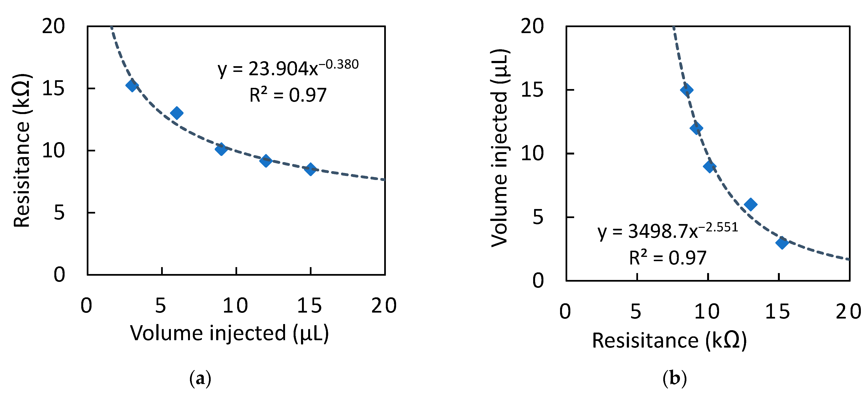
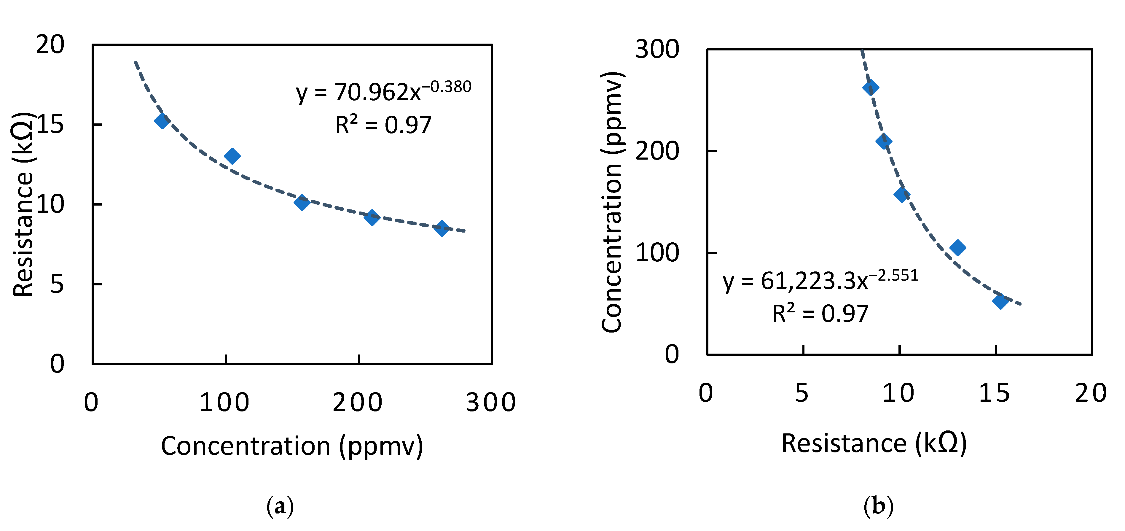
Varying volumetric amounts of each of the three solvents were added to the container for evaporation, and five steady-state resistance readings per solvent were collected and plotted. The relation between volumetric amounts and resistance values is shown in Figure 1. The obtained resistance data from the A3 monitor were fitted into a nonlinear curve using a power function (y = a·xb), where R2 represents the squared correlation coefficient. As expected, the resistance values decreased with the increasing amount of acetone, as observed in Figure 1a. In the presence of a volatile compound, the MOx sensor reacts with the compound, reducing the oxygen on the surface of the metal oxide. Thus, the electrical current flow increases, which is coupled with the resistance values decreasing [19]. The data were then plotted with the axes reversed, as in Figure 1b, and this enabled obtaining a predictive expression to be later used in the model development (Section 3.4), whereby the injected volume amount could be deduced from the resistance measurement. It can be seen that the data fitting to the power law, within the limits tested, was very good as the correlation coefficient value is high, close to 1. Moreover, the volumetric values (of injected liquid) were converted to ppmv values (of evaporated solvent vapour) for further modeling purposes; the relation between concentration in ppmv and resistance values are presented in Figure 2 for the case of acetone. The trends of the curves in Figure 1 and Figure 2 are comparable, as expected.
The same type of experiments was conducted using ethanol and n-hexane, and the results are presented in Figures S3–S10 in the Supplementary Materials. The resistance values of ethanol and hexane are greater than those of acetone (8.5 to 15.2 kΩ), ranging from 13.6 to 25.7 kΩ for ethanol and 43.5 to 104.2 kΩ for n-hexane. At the same time, it should be accounted that the molecular weights of these solvents differ, and therefore, the vapour concentration ranges also somewhat differed: 52.5 to 262.5 ppmv for acetone; 67.0 to 335.0 ppmv for ethanol; 29.5 to 147.6 ppmv for n-hexane. Still, the trends of the fitted curves are similar for all three solvents, but the fitted coefficients (a and b) differed, pointing to different levels of interaction between the vapour molecules and the MOx sensor. For instance, it is plausible that acetone is likely to interact more strongly with the SnO2-based sensor. This could be explained by density functional theory calculations that show that acetone molecules act as donors to transfer electrons and can be adsorbed on Sn and oxygen vacancy sites [31]. Given that the resistance values of these three compounds range differently, this behavior is posed to be useful for identifying and quantifying the VOC composition more efficiently, as will be detailed in the model development (Section 3.4).
3.2. Double Volatile Organic Compounds
From conducting the experiments of single VOCs, resistance ranges of all three VOCs were confirmed under controlled conditions, indicating the response of the sensor when it is exposed to a particular VOC. However, there are diverse VOCs that exist in real monitoring circumstances. Therefore, it is essential to investigate how the monitor would respond when two mixed VOCs were inserted into the sealed container. Another objective is also to test the selectivity/sensitivity of the MOx sensor in the A3 monitor. Table 1 lists the volumetric amounts and vapour concentrations of acetone and ethanol in the double solvent experiments, along with the total vapour concentrations (sum of the two solvents), and measured resistance values from each experiment. Similar experiments were also conducted for acetone + n-hexane and for ethanol + n-hexane experiments; all measured data (including preliminary and calibration trials) can be found in Thakor [32].
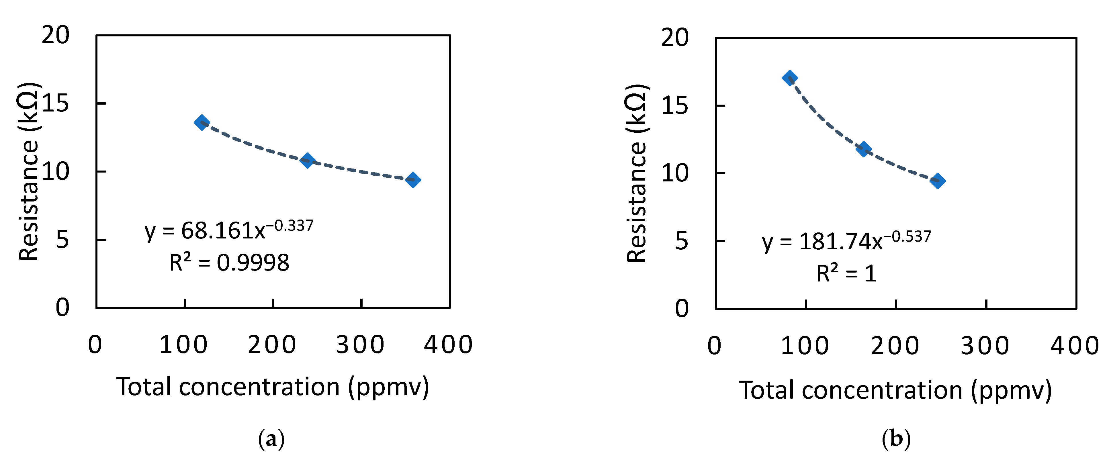
Figure 3 shows the relation between total vapour concentration, in calculated ppmv, and resistance values in the presence of acetone + ethanol combination (in Figure 3a), and acetone + n-hexane (in Figure 3b). It is found that the resistance values in the presence of a second VOC (9.4 to 17.0 kΩ) were close to the values previously presented for single acetone (in the range of 10.1 to 15.2 kΩ, for the comparable range of 3 to 9 μL acetone), which signifies that acetone has a dominant effect on MOx sensor resistance. Therefore, it is again suggested that acetone is more likely to attach to the sensor, compared to the other two compounds [31]. The relation between the combination of ethanol and n-hexane and resistance values is plotted and illustrated in Figure S11, and it is shown that the resistance values (15.3 to 25.3 kΩ) lean towards the single ethanol condition (16.7 to 25.7 kΩ). It is thus confirmed that the MOx sensor resistance values of the A3 monitor are unequally influenced by the type of VOC, and the influence degree, from strongest to weakest, is in the following order: acetone > ethanol > n-hexane.
3.3. Correlation of Single and Double VOC Results
As discussed previously, the relationships between resistance values and vapour concentrations for the conditions of a single VOC or double VOCs in combination have been given. In this section, these relationships are compared (i.e., a single compound versus the same compounds with another VOC), and the aim is to obtain correlations between these sets of data. The further aim is to provide insight into the influence of a second VOC on the measured resistance values. These correlations are needed for the mathematical model developed in Section 3.4.
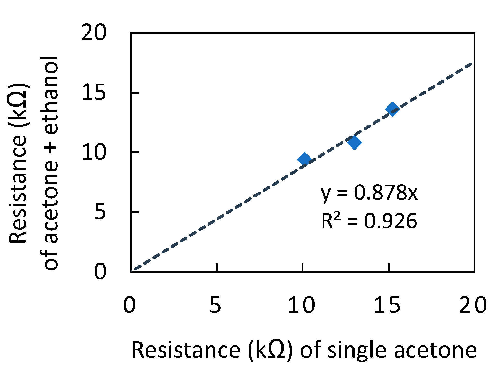
In Figure 4, it can be observed that resistance values from the experiments with single acetone are proportionally correlated (according to an adequate fit of a linear equation with zero intercepts) with those of acetone + ethanol condition. The slope coefficient of this fitted equation is 0.878, which is less than 1. As expected, this indicates that the presence of ethanol in combination with acetone leads to depressing the resistance values of the MOx sensor further. The deviation of this slope value from 1 is an indication of the strength of the second solvent in altering the resistance value beyond that of the single first solvent. As it has been asserted that acetone exerts more influence on resistance than ethanol does, it is understandable that the slope value is smaller but still close to 1.
The coefficients of each binary combination (acetone + ethanol; acetone + n-hexane; ethanol + n-hexane) are listed in Table 2. Notable from this table are the two slope coefficients at the extremes. The value of 1.009 for the acetone + n-hexane case (i.e., dual solvent values correlated to single acetone case), is essentially equal to 1, and this signifies that, at similar concentrations (equivolumetric but slightly richer in acetone ppmv-wise), n-hexane is undetectable when in combination with acetone. The value of 0.168 for the reverse case, n-hexane + acetone (i.e., dual solvent values correlated to single n-hexane values), confirms that acetone influence overwhelms the MOx sensor, reducing sensitivity to n-hexane. Yet, this value being sufficiently larger than zero still suggests that when the n-hexane concentration sufficiently exceeds that of acetone, detection of the dual solvent effect would still be possible. Altogether, the data in Table 2, once again, suggest that acetone influences the resistance more strongly than ethanol, followed by n-hexane, which is consistent with the findings in Section 3.2. These correlation equations are used in Section 3.4 for the prediction of mixed VOC composition and mathematical model development.
3.4. Predictive Mathematic Model: Development and Simulation
As aforementioned, the A3 monitor uses a linear model to convert the measured resistance data from the MOx sensor directly into a VOC-based AQI value. However, it has been shown in previous results sections that the relationship between resistance values and vapour concentrations of VOCs is nonlinear (i.e., follows a power–law relationship). Therefore, it is necessary to develop a mathematical model to improve the interpretation of the MOx sensor’s data, both with regard to estimating composition and yielding a useful AQI reading. The predictive mathematical model developed and presented herein aims to first estimate the total concentration of VOCs and subsequently estimate the composition of individual VOCs in the sampled air.
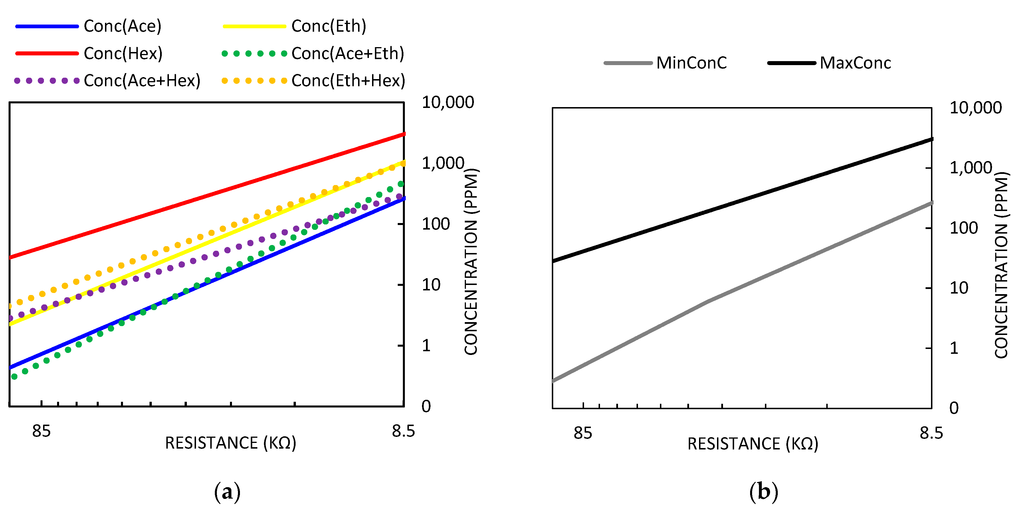
According to the resistance versus concentration equations experimentally fitted in Section 3.1 and Section 3.2, Figure 5a was prepared by plotting calculated values of concentration for resistance values ranging from 1 to 200 kΩ. By using logarithmic scales, it was observed that all data series became linear. Moreover, it was observed that the single solvent n-hexane line lied higher than other lines and that the acetone single solvent line lied lower than other lines (except at high resistance values, which correspond to low concentrations, where acetone–ethanol became the lowest line). These trends suggest that at a given resistance value, concentrations are bound between a high and a low value. On this basis, the data used to generate Figure 5a were replotted, taking only the maximum and the minimum value at any given resistance, as shown in Figure 5b. These maximum and minimum lines are taken as upper and lower bounds that limit the range of possible concentrations for any measured resistance value when analysing an air sample containing one or more of the three studied VOCs.
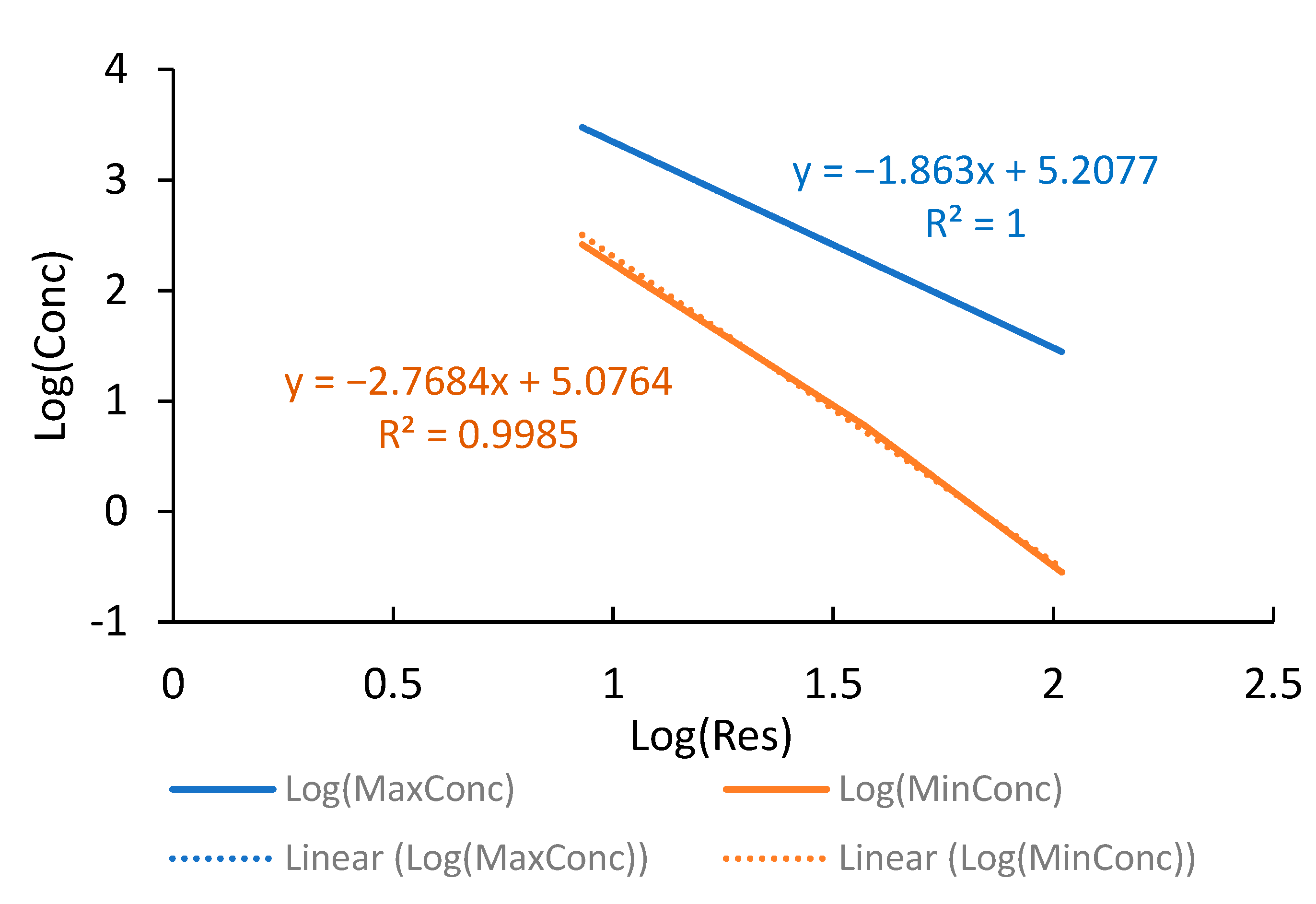
In Figure 6, the calculated values that make up the maximum and minimum lines shown in Figure 5b were converted into logarithmic values (i.e., log(Res) versus log(Conc)), and line equations were fitted to each data series. The aim was to enable calculating the maximum and minimum total concentration value for a given measured resistance value. This provides a range of possible total concentrations, but to arrive at a single estimated value, and eventually VOC composition, additional correlations are needed, as presented next.
The equations from both lines in Figure 6 have nearly identical intercepts (i.e., 5.2077 and 5.0764), but the slopes are substantially different. Similarly, looking at Figure 5a, it can be seen that single solvent lines for n-hexane, ethanol, and acetone have different slopes. These observations were used to conceptualise that for the mathematical algorithm to predict the exact concentration between the upper- and lower-bound values for a given measured resistance, it is needed to know on what line with what slope the measured air would lie if its concentration was varied to produce multiple resistance values. Given that with two points on a graph it is possible to determine the slope, the idea of sample dilution was conceived. If the resistance value of the original air and of a diluted air (of known dilution factor) are known, and their log values taken, then two x-values on Figure 6 are known. However, the y-values are not known. Yet, it was noticed that the ratio between two resistance values can be compared to the ratios of two resistance values that lie on the maximum and the minimum lines. This is detailed in Table 3.
For physically implementing the approach of using a diluted sample for obtaining a second value of MOx sensor resistance, it would be required to have the pollutant monitor perform two sequential measurements—one with the diluted air and another with undiluted air. One way of doing this would for the air quality monitor to possess a small compressed air canister for supplying clean dilution air; evidently, the measurement frequency would be limited by the capacity of the canister, which likely would have to be enough for 24 h of continuous measurement.
In Table 3, it was hypothesised that an air sample containing 200 ppmv of VOCs was measured, and the same sample four times diluted (i.e., containing 50 ppmv) was also measured. If the composition of this air sample was such that the data points would lie along the maximum line, log values of the maximum possible measured resistance were calculated using the equations given in Figure 6. Likewise, if the composition of this air sample was such that the data points would lie along the minimum line, log values of the minimum possible measured resistance were calculated using the equations given in Figure 6. The resistance values were then calculated from the log values, as shown in Table 3. The ratio between the maximum resistance values is 2.105, and the ratio between the minimum resistance values is 1.650. Thus, it is posed that for any measured air sample and its four-times-diluted sample, the ratio between measured resistance would lie between 1.650 and 2.105. Once it is known what the ratio is, it is then possible to determine the line equation that falls between the maximum and minimum lines in Figure 6 and finally estimate the total VOC concentration of the original undiluted air sample. This is exemplified next.
The ratio of the two resistance values from the corresponding diluted and original samples (D/O ResRatio) is used to find the slope and intercept values of the line equation that falls onto Figure 6. This is accomplished through an interpolation method, as exemplified in Table 4. For example, assume that for a certain air sample, the resistance values of the original sample and the four-times-diluted sample are at 10 and 20 kΩ, respectively, which is reasonable as the resistance value of the diluted sample must be lower given the lower concentration of VOC. The resistance ratio (ResRatio) of this set of measurements is 2.200, as listed in Table 4. The slope and intercept of the line equation that runs through these two points are obtained by interpolating the slope (D) and intercept (E) of the maximum and minimum lines. In this Table 4 example, the resulting equation becomes log(Conc) = −2.071·log(Res) + 5.178. Therefore, the original sample resistance is then used to calculate the original sample concentration; for 10 kΩ this corresponds to 1277 ppmv. Had the four-times-diluted resistance been 19, 18, and 17 kΩ, the smaller resistance difference between original and diluted signifies a less concentrated original air, and the interpolation procedure would lead to total VOC concentration estimates of 756, 447, and 264 ppmv, respectively. This approach can be used to determine the total VOC concentration of any air sample in which original and four-times-diluted concentration lies within the graphical area of Figure 5.
After estimating the total original concentration of VOCs using the dilution, D/O ResRatio, and slope interpolation method presented above, it is important to attain estimates of the individual VOC composition to provide valuable information for air pollutant monitoring. As observed in Figure 5a,b, the maximum resistance values, at any given concentration and for single compounds, are attributable to n-hexane, while the minimum resistance values are attributable to acetone. Therefore, it can be logically inferred that the concentration order of different VOC combinations, based on the D/O ResRatio, is as listed in Table 5.
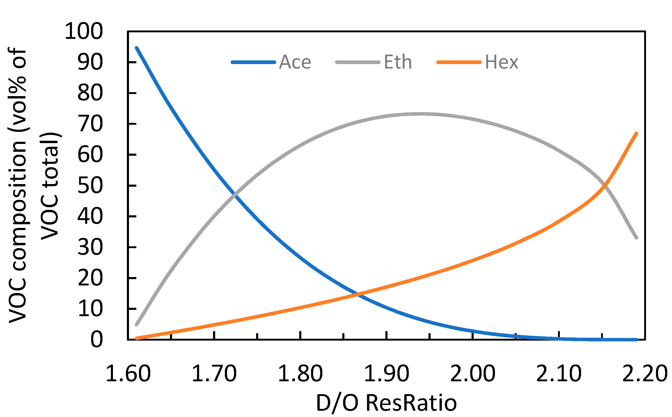
Relating the D/O ResRatio to VOC composition, the logical classification of Table 5 states that n-hexane is enriched in the composition when the resistance ratio is closer to, or exceeding the “maximum value” (2.10), while acetone is enriched in the composition when the resistance ratio approaches or surpasses the “minimum value” (1.65). Therefore, trends of the composition of acetone and hexane should be opposite, with ethanol contributing primarily to the composition of samples with intermediate resistance ratios; this is illustrated in the compositional graph, based on volume percent of total VOC concentration, in Figure 7. To plot the graph in Figure 7, empirical equations are introduced to define the trends. The empirical equations are generated with the precept that the sum of the volumetric fractions of the three components should be 100% of the total VOC concentration. Next, we discuss how the empirical equations are generated.
It is noted that the coefficient values listed in Table 2 demonstrate the degree of VOC interaction with the MOx sensor, and this information is herein used in the formation of empirical equations to estimate the composition of VOC. To arrive at the curves plotted in Figure 7, obeying the logic presented in Table 5, Equations (1)–(3) are proposed to provide an estimated composition based on a measure D/O ResRatio value. Given that ethanol is associated with intermediate ResRatio values, it was also herein treated as the balanced compound (according to Equation (3)), making up the sum of the three equations to 100%. Moreover, to compose Equations (1) and (2), the coefficients from Table 2 that relate ethanol to the other two compounds were used. The coefficient of Ace+Eth (0.878), which is associated with the strength of acetone, was divided by the value of the coefficient of Eth+Ace (0.538), which is associated with the strength of ethanol, to yield a value of 1.6325, and this was incorporated into Equation (1) and termed Ace+Eth. The same approach was applied in taking the Eth+Hex value (0.939) and dividing it by the Hex+Eth value (0.254) to yield a value termed Eth/Hex with a value of 3.6991. Comparing these two values (1.6325 and 3.6991), it is evident that the value involving ethanol and n-hexane is much larger than that involving ethanol and acetone, which impacted the shape of the empirical curves in Figure 7, being asymmetrically shifted towards the acetone-rich side (i.e., mixtures containing acetone has a narrower range of smaller ResRatio values, and mixtures containing substantial amounts of n-hexane cover a wider range of higher ResRatio values). The other numerical coefficients used in Equations (1) and (2) were selected to reasonably shape the curves in Figure 7 but can be modified if experimentally validated data calls for different values. Experimental validation was not accomplished in the present study as the COVID-19 pandemic lockdowns in 2020 forced the study to conclude before such experiments could be conducted.
As an example of the application of Equations (1)–(3), the previously presented hypothetical values of measured original and diluted resistances, namely, 10 kΩ and 17 to 20 kΩ, can be used to generate VOC compositions. In the same order of resistance ratios (20/10, 19/10, 18/10, 17/10), the equations yield compositional values of 145.8, 118.9, 78.6, and 35.4 ppmv for acetone; 105.9, 281.6, 547.8, and 913.6 ppmv for ethanol; 12.7, 46.4, 129.1, and 328.2 ppmv for n-hexane. Thus, these types of air would have been deemed to be especially rich in ethanol, somewhat rich in n-hexane, and lean in acetone.
In addition to the assumptions, simplifications, and logical decisions used to generate the mathematical model (i.e., Equations (1)–(3), which should be revisited in any future further development and implementation of the proposed methodology for using a single MOx sensor to delineate the composition of a mixture of three VOC compounds), there are also some important limitations in the model that should be noted and possibly eliminated in future endeavors. It can be seen from Figure 7 that ethanol is predicted to be always present in samples with ResRatio values between 1.60 and 2.20, even though at the outer limits of this range, it is very much possible that binary mixtures of acetone and n-hexane could have such ResRatio values. Another clear limitation from Figure 7 is that the model predicts that any VOC mixtures with ResRatio value between 1.60 and 2.20 will not contain more than approximately 73 vol% of ethanol in combination with acetone and n-hexane; this once again creates limitations when sensing binary VOC mixtures instead of ternary mixtures. Such limitation is a product of the coefficients used in Equations (1) and (2), which, as aforementioned, should be experimentally validated, and the construct of these equations, which could be further tuned to reshape the curves, as dictated by experimental validation of ternary mixtures. Temperature and humidity corrections, either to measured values or to equation coefficients, would need to be taken into account for use of the proposed model under uncontrolled ambient conditions.
Though the proposed mathematical model has limitations and uncertainties, it does provide approximate trends and values of individual VOCs in VOC mixtures. With the development of this model, we move one step closer to enabling the use of single MOx sensors in mobile air pollutant monitors to evaluate if any sensed VOC may be exceeding the threshold of a defined standard. As concluded by Collier-Oxandale et al. [9], the low cost and low barrier to deployment of MOx sensors can facilitate studies in the domains of public health research and environmental justice, including the assessment of the impact of VOC sources on overburdened communities. They also point out that, in the context of limited resources in such communities for such studies, even cursory data on VOC emissions and immissions can be of value and can complement the more cumbersome and costly conventional approaches to VOC monitoring.
The output of the proposed model, once volumetric percentages are multiplied by total ppmv value, are ppmv values of individual VOC, and these can be used to calculate a VOC-based AQI. Garcia et al. [33] have worked on expressing AQI of VOC-laden air to provide information on VOC pollution in an area. The air quality index for VOCs (AQIVOC) is weighed based on the impact of each VOC according to environmental regulations. They assigned an environmental impact coefficient (α) to each VOC, which is correlated to their emission limit values. For example, an α value of 1 correlates to an immision limit of 600 mg/Nm3, and an α value of 120 correlates to an immision limit of 5 mg/Nm3, according to Italian regulations [33]. The equation for AQIVOC, for air containing three VOC compounds, would then be given by the following:
where αi is the environmental impact coefficient, and νi is the atmospheric concentration in the analysed air of the i-th VOC.
If more than three solvent vapours are present in the polluted air, at concentrations that affect the resistance readings taken by a single MOx sensor, it may be necessary to use more than one sensor, in such a manner that different sensors are more sensitive to particular classes of volatile organics. The ability to discern more than three VOC can, in certain situations, provide a more accurate representation of the AQIVOC; for instance, the original AQIVOC equation presented in Garcia et al. [33] uses i = 18, signifying that there were 18 VOCs of interest in their study, namely, benzene, chloroform, cyclohexane, 1,2-dichlorobenzene, dichloromethane, ethylbenzene, heptane, hexane, methylcyclohexane, methylcyclopentane, 2-methylhexane, 2-methylpentane, toluene, tetrachloroethylene, trichloroethylene, 1,2,4-trimethylbenzene, and (m- p- o-)xylene. The necessity of the present composition determination approach to detect three VOCs with differing interaction strength with the MOx sensor may be seen as an additional limitation of the approach, but this is a general limitation of MOx sensors, which are designed primarily to detect total VOC concentration, made equivalent to a particular VOC (e.g., n-hexane), rather than to determine VOC composition.
4. Conclusions
This paper presents an approach to improving the accuracy of AQI determination when using a single MOx sensor, as is the case of the tested uRAD A3 mobile monitor. This was accomplished by building a mathematical model to estimate the composition of VOCs in a ternary mixture. Experiments were conducted with single VOC and double VOC combinations, and results were plotted and fitted into specific curves and used to obtain coefficients. The experimental data indicated that the resistance values varied with different VOCs at the same concentrations, and moreover, that for the three tested VOCs the resistance values ranged between an upper and lower limit, which could be represented by linear equations on a log(Res) versus log(Conc) graph. These experimental results were used to create a predictive mathematical model, and the preliminary results demonstrate the feasibility of applying the discrepancy in VOC-MOx sensor interaction among the three VOCs to develop such a model. It could be concluded that acetone most strongly interacted with the MOx sensor, followed by ethanol, and then by n-hexane. A hypothetical approach where the resistances of the original air sample and a four-times-diluted air sample are measured was employed to define a linear equation as a function of the D/O ResRatio, to then obtain the original total VOC concentration (exemplified in Table 4). According to the analysis of coefficients between single VOC and double VOC experiments, it was found that the interaction performance of ethanol with the MOx sensor is slightly closer to acetone, while hexane shows more dissimilarity to ethanol. These behaviors and coefficient ratio values were used to conceptualise empirical equations (Equations (1)–(3)) whose curves as a function of ResRatio yielded expected VOC composition data (exemplified in Figure 7). Overall, the results of this mathematical model are divided into two parts to fulfill the study’s aims, as follows: (i) determining the total concentration of VOCs with the resistance values obtained from original and diluted samples and (ii) estimating individual VOC composition in the original sampled air. Once a VOC composition is known, it is then possible to calculate an estimated AQIVOC value, according to Equation (4).
Improving the representation of the air quality index has far-reaching importance in daily life as VOC pollutants are present in the outside environment, but they are also indoor pollutants. Many of them are in offices, homes, and industrial facilities. Hence, pollutants are in close vicinity of populations, which makes them vulnerable to inhale significant quantities that can exceed recommended or regulated health limits. Air pollutants continue to cause many health problems and long-term health effects; therefore, knowing the air quality and controlling it continues to gain importance every day and is a pressing societal need.
Supplementary Materials
The following are available online at https://0-www-mdpi-com.brum.beds.ac.uk/article/10.3390/cleantechnol3030031/s1: Figures S1–S11.
Author Contributions
Conceptualisation, R.M.S.; methodology, G.S.T. and R.M.S.; investigation, G.S.T.; resources, R.M.S.; writing—original draft preparation, G.S.T. and N.Z.; writing—review and editing, R.M.S.; supervision, R.M.S. All authors have read and agreed to the published version of the manuscript.
Funding
This research did not receive external funding.
Data Availability Statement
The data presented in this study are available on request from the corresponding author.
Acknowledgments
The authors would like to thank Radu Motisan from Magnasci SRL for providing support with the use of the uRAD A3 monitor and the uRADMonitor dashboard. The authors are also thankful for the assistance provided by laboratory technician Jacqueline Fountain and Piaoyu Hu with the planning of laboratory experiments, and Ashutosh Singh for advice on data analysis methods.
Conflicts of Interest
The authors declare no conflict of interest.
References
- Itoh, T.; Akamatsu, T.; Izu, N.; Shin, W.; Byun, H.-G. Monitoring of disease-related volatile organic compounds in simulated room air. IEEE Sens. Proc. 2014, 1427–1430. [Google Scholar] [CrossRef]
- Karuppuswami, S.; Wiwatcharagoses, N.; Kaur, A.; Chahal, P. Capillary Condensation Based Wireless Volatile Molecular Sensor. In Proceedings of the 2017 IEEE 67th Electronic Components and Technology Conference (ECTC), Orlando, FL, USA, 30 May–2 June 2017; pp. 1455–1460. [Google Scholar]
- Fu, J.L.; Ayazi, F. High- Q AlN-on-Silicon Resonators with Annexed Platforms for Portable Integrated VOC Sensing. J. Microelectromech. Syst. 2015, 24, 503–509. [Google Scholar] [CrossRef]
- Collier-Oxandale, A.; Wong, N.; Navarro, S.; Johnston, J.; Hannigan, M. Using gas-phase air quality sensors to disentangle potential sources in a Los Angeles neighborhood. Atmos. Environ. 2020, 233, 117519. [Google Scholar] [CrossRef]
- Szczurek, A.; Maciejewska, M. Assessment of VOCs in air using sensor array under various exposure conditions. In Proceedings of the 2012 IEEE Sensors Applications Symposium Proceedings, Brescia, Italy, 7–9 February 2012; pp. 1–5. [Google Scholar]
- Nazemi, H.; Joseph, A.; Park, J.; Emadi, A. Advanced Micro- and Nano-Gas Sensor Technology: A Review. Sensors 2019, 19, 1285. [Google Scholar] [CrossRef] [PubMed] [Green Version]
- Ghosh, R.; Gardner, J.W.; Guha, P.K. Air Pollution Monitoring Using Near Room Temperature Resistive Gas Sensors: A Review. IEEE Trans. Electron Devices 2019, 66, 3254–3264. [Google Scholar] [CrossRef]
- Gao, H.; Guo, J.; Li, Y.; Xie, C.; Li, X.; Liu, L.; Chen, Y.; Sun, P.; Liu, F.; Yan, X.; et al. Highly selective and sensitive xylene gas sensor fabricated from NiO/NiCr2O4 p-p nanoparticles. Sens. Actuators B Chem. 2019, 284, 305–315. [Google Scholar] [CrossRef]
- Collier-Oxandale, A.M.; Thorson, J.; Halliday, H.; Milford, J.; Hannigan, M. Understanding the ability of low-cost MOx sensors to quantify ambient VOCs. Atmos. Meas. Tech. 2019, 12, 1441–1460. [Google Scholar] [CrossRef] [Green Version]
- Wang, C.; Yin, L.; Zhang, L.; Xiang, D.; Gao, R. Metal Oxide Gas Sensors: Sensitivity and Influencing Factors. Sensors 2010, 10, 2088–2106. [Google Scholar] [CrossRef] [PubMed] [Green Version]
- Srivastava, A. Detection of volatile organic compounds (VOCs) using SnO2 gas-sensor array and artificial neural network. Sens. Actuators B Chem. 2003, 96, 24–37. [Google Scholar] [CrossRef]
- Lee, D.; Tae, Y.; Huh, J.; Lee, D. Fabrication and characteristics of SnO2 gas sensor array for volatile organic compounds recognition. Thin Solid Films 2002, 416, 271–278. [Google Scholar] [CrossRef]
- Liu, X.; Cheng, S.; Liu, H.; Hu, S.; Zhang, D.; Ning, H. A Survey on Gas Sensing Technology. Sensors 2012, 12, 9635–9665. [Google Scholar] [CrossRef] [PubMed] [Green Version]
- Ahmad, R.; Majhi, S.M.; Zhang, X.; Swager, T.M.; Salama, K.N. Recent progress and perspectives of gas sensors based on vertically oriented ZnO nanomaterials. Adv. Colloid Interface Sci. 2019, 270, 1–27. [Google Scholar] [CrossRef] [PubMed]
- Chavali, M.S.; Nikolova, M.P. Metal oxide nanoparticles and their applications in nanotechnology. SN Appl. Sci. 2019, 1, 607. [Google Scholar] [CrossRef] [Green Version]
- Lin, T.; Lv, X.; Hu, Z.; Xu, A.; Feng, C. Semiconductor Metal Oxides as Chemoresistive Sensors for Detecting Volatile Organic Compounds. Sensors 2019, 19, 233. [Google Scholar] [CrossRef] [Green Version]
- Maduraiveeran, G.; Sasidharan, M.; Jin, W. Earth-abundant transition metal and metal oxide nanomaterials: Synthesis and electrochemical applications. Prog. Mater. Sci. 2019, 106, 100574. [Google Scholar] [CrossRef]
- Mirzaei, A.; Lee, J.-H.; Majhi, S.M.; Weber, M.; Bechelany, M.; Kim, H.W.; Kim, S.S. Resistive gas sensors based on metal-oxide nanowires. J. Appl. Phys. 2019, 126, 241102. [Google Scholar] [CrossRef] [Green Version]
- Di Lecce, V.; Calabrese, M.; Dario, R. Computational-based volatile organic compounds discrimination: An experimental low-cost setup. In Proceedings of the 2010 IEEE International Conference on Computational Intelligence for Measurement Systems and Applications, Taranto, Italy, 6–8 September 2010; pp. 54–59. [Google Scholar]
- Alinoori, A.H.; Masoum, S. Multicapillary Gas Chromatography—Temperature Modulated Metal Oxide Semiconductor Sensors Array Detector for Monitoring of Volatile Organic Compounds in Closed Atmosphere Using Gaussian Apodization Factor Analysis. Anal. Chem. 2018, 90, 6635–6642. [Google Scholar] [CrossRef]
- Choi, Y.M.; Cho, S.; Jang, D.; Koh, H.-J.; Choi, J.; Kim, C.-H.; Jung, H.-T. Ultrasensitive Detection of VOCs Using a High-Resolution CuO/Cu2O/Ag Nanopattern Sensor. Adv. Funct. Mater. 2019, 29, 1808319. [Google Scholar] [CrossRef]
- Leidinger, M.; Sauerwald, T.; Conrad, T.; Reimringer, W.; Ventura, G.; Schütze, A. Selective Detection of Hazardous Indoor VOCs Using Metal Oxide Gas Sensors. Procedia Eng. 2014, 87, 1449–1452. [Google Scholar] [CrossRef] [Green Version]
- Lee, D.D.; Lee, D.S. Environmental gas sensors. IEEE Sens. J. 2002, 1, 214–224. [Google Scholar]
- Masson, N.; Piedrahita, R.; Hannigan, M. Approach for quantification of metal oxide type semiconductor gas sensors used for ambient air quality monitoring. Sens. Actuators B Chem. 2015, 208, 339–345. [Google Scholar] [CrossRef]
- Yurko, G.; Roostaei, J.; Dittrich, T.; Xu, L.; Ewing, M.; Zhang, Y.; Shreve, G. Real-Time Sensor Response Characteristics of 3 Commercial Metal Oxide Sensors for Detection of BTEX and Chlorinated Aliphatic Hydrocarbon Organic Vapors. Chemosensors 2019, 7, 40. [Google Scholar] [CrossRef] [Green Version]
- Air-Quality Gas Sensor. Available online: https://www.winsen-sensor.com/d/files/MP503.pdf (accessed on 24 February 2021).
- uRADMonitor A3. Available online: https://www.uradmonitor.com/wordpress/wp-content/uploads/2020/01/a3_datasheet_v108_en.pdf (accessed on 24 February 2021).
- Air Quality Sensor Test Results with Raspberry Pi. Available online: https://www.switchdoc.com/2016/06/air-quality-sensor-tested-raspberry-pi/ (accessed on 26 March 2021).
- Motisan, R.; Santos, R.M. Mobility and Measurement Tackle Ongoing Challenge of Air Pollution. Canadian Chemical News 2018, March. Available online: https://www.cheminst.ca/magazine/article/mobility-and-measurement-tackle-ongoing-challenge-of-air-pollution/ (accessed on 24 February 2021).
- Annanouch, F.-E.; Bouchet, G.; Perrier, P.; Morati, N.; Reynard-Carette, C.; Aguir, K.; Bendahan, M. How the Chamber Design Can Affect Gas Sensor Responses. Proceedings 2018, 2, 820. [Google Scholar] [CrossRef] [Green Version]
- Chen, Y.; Qin, H.; Cao, Y.; Zhang, H.; Hu, J. Acetone Sensing Properties and Mechanism of SnO2 Thick-Films. Sensors 2018, 18, 3425. [Google Scholar] [CrossRef] [PubMed] [Green Version]
- Thakor, G.S. Testing and Validation of Mobile Air Quality Monitor for Sensing and Delineating VOC Emissions. Master’s Thesis, University of Guelph, Guelph, ON, Canada, 2020. Available online: http://hdl.handle.net/10214/17941 (accessed on 26 February 2021).
- Astiaso, D.; Cumo, F.; Gugliermetti, F. Air Quality in Portal Areas: An Index for VOCs Pollution Assessment. In Air Quality–New Perspective; IntechOpen: London, UK, 2012. [Google Scholar] [CrossRef] [Green Version]
Figure 1.
(a) The effect of acetone concentration, expressed as volume of injected solvent, on the MOx sensor’s resistance value; (b) the inversed plot of resistance versus injected volume. All data points are averages of five replicates.
Figure 1.
(a) The effect of acetone concentration, expressed as volume of injected solvent, on the MOx sensor’s resistance value; (b) the inversed plot of resistance versus injected volume. All data points are averages of five replicates.

Figure 2.
(a) The effect of acetone concentration, expressed as concentration (ppmv) of evaporated solvent, on the MOx sensor’s resistance value; (b) the inversed plot of resistance versus concentration. All data points are averages of five replicates.
Figure 2.
(a) The effect of acetone concentration, expressed as concentration (ppmv) of evaporated solvent, on the MOx sensor’s resistance value; (b) the inversed plot of resistance versus concentration. All data points are averages of five replicates.

Figure 3.
(a) Measured resistance values in the presence of equivolumetric mixtures of acetone and ethanol; (b) measured resistance values in the presence of equivolumetric mixtures of acetone and n-hexane.
Figure 3.
(a) Measured resistance values in the presence of equivolumetric mixtures of acetone and ethanol; (b) measured resistance values in the presence of equivolumetric mixtures of acetone and n-hexane.

Figure 4.
Single (acetone) versus double (equivolumetric acetone + ethanol) VOCs correlation equations; each data point corresponds to experiments performed using the same solvent volume of the primary VOC.
Figure 4.
Single (acetone) versus double (equivolumetric acetone + ethanol) VOCs correlation equations; each data point corresponds to experiments performed using the same solvent volume of the primary VOC.

Figure 5.
(a) Single and double VOCs resistance (Res) versus concentration (Conc) calculated curves (from experimentally fitted equations), plotted on logarithmic scales to yield linear correlations; (b) maximum and minimum values from Figure 5a replotted as two limiting upper and lower bounds.
Figure 5.
(a) Single and double VOCs resistance (Res) versus concentration (Conc) calculated curves (from experimentally fitted equations), plotted on logarithmic scales to yield linear correlations; (b) maximum and minimum values from Figure 5a replotted as two limiting upper and lower bounds.

Figure 6.
Maximum and minimum concentrations curves, replotted as log(Res) versus log(Conc) and fitted to linear equations.
Figure 6.
Maximum and minimum concentrations curves, replotted as log(Res) versus log(Conc) and fitted to linear equations.

Figure 7.
Empirical curves of individual VOC composition across a range of D/O resistance ratios.


Table 1.
Acetone and ethanol dual solvent amounts, vapour concentrations, and measured resistance values.
Table 1.
Acetone and ethanol dual solvent amounts, vapour concentrations, and measured resistance values.
| Exp. | A 1 Vol (µL) | A 1 Conc (ppmv) | E 1 Vol (µL) | E 1 Conc (ppmv) | Total Vol (µL) | Total Conc (ppmv) | Resistance (kΩ) |
|---|---|---|---|---|---|---|---|
| 1 | 3 | 52.50 | 3 | 66.99 | 6 | 119.49 | 13.59 |
| 2 | 6 | 104.99 | 6 | 133.98 | 12 | 238.97 | 10.81 |
| 3 | 9 | 157.49 | 9 | 200.97 | 18 | 358.46 | 9.38 |
1 A, acetone; E, ethanol.
Table 2.
Coefficients of binary combinations.
| Single | Acetone | Ethanol | n-Hexane | |||
|---|---|---|---|---|---|---|
| Double | Ace+Eth | Ace+Hex | Eth+Ace | Eth+Hex | Hex+Ace | Hex+Eth |
| Slope coefficient | 0.878 | 1.009 | 0.538 | 0.939 | 0.168 | 0.254 |
Table 3.
Logarithmic values of concentrations and resistance values of VOCs.
| Con (ppm) | Log(Con) | Log(ResMax) | Log(ResMin) | ResMax (kΩ) | ResMin (kΩ) |
|---|---|---|---|---|---|
| 200 | 2.30 | 1.56 | 1.00 | 36.32 | 10.06 |
| 50 | 1.70 | 1.88 | 1.22 | 76.45 | 16.60 |
Table 4.
Log concentrations, log resistance values, and interpolation of resistance ratio.
| Data Set | D/O ResRatio | Log(Con) = D·Log(Res)+E | ||
|---|---|---|---|---|
| Slope D | Intercept E | |||
| 1 | Maximum | 2.105 | −1.863 | 5.208 |
| 2 | Minimum | 1.650 | −2.768 | 5.077 |
| 3 | Hypothetical (20 kΩ/10 kΩ) | 2.000 | −2.071 1 | 5.178 1 |
1 These values are interpolated based on the measured D/O ResRatio, compared to the maximum and minimum lines’ D/O ResRatio.
Table 5.
Modelling logic for determining the composition of VOCs based on a measured D/O ResRatio.
| Measured D/O ResRatio | Acetone Concentration | n-Hexane Concentration | Ethanol Concentration |
|---|---|---|---|
| <1.75 | Highest | Lowest | Acetone > Ethanol > Hexane |
| >2.15 | Lowest | Highest | Acetone < Hexane < Ethanol |
| 1.75–2.15 | Acetone < Hexane | Hexane < Ethanol | Highest |
Publisher’s Note: MDPI stays neutral with regard to jurisdictional claims in published maps and institutional affiliations. |
© 2021 by the authors. Licensee MDPI, Basel, Switzerland. This article is an open access article distributed under the terms and conditions of the Creative Commons Attribution (CC BY) license (https://creativecommons.org/licenses/by/4.0/).
Share and Cite
MDPI and ACS Style
Thakor, G.S.; Zhang, N.; Santos, R.M. Sensing and Delineating Mixed-VOC Composition in the Air Using a Single Metal Oxide Sensor. Clean Technol. 2021, 3, 519-533. https://0-doi-org.brum.beds.ac.uk/10.3390/cleantechnol3030031
AMA Style
Thakor GS, Zhang N, Santos RM. Sensing and Delineating Mixed-VOC Composition in the Air Using a Single Metal Oxide Sensor. Clean Technologies. 2021; 3(3):519-533. https://0-doi-org.brum.beds.ac.uk/10.3390/cleantechnol3030031
Chicago/Turabian StyleThakor, Govind S., Ning Zhang, and Rafael M. Santos. 2021. "Sensing and Delineating Mixed-VOC Composition in the Air Using a Single Metal Oxide Sensor" Clean Technologies 3, no. 3: 519-533. https://0-doi-org.brum.beds.ac.uk/10.3390/cleantechnol3030031