Time- and Frequency-Domain Steady-State Solutions of Nonlinear Motional Eddy Currents Problems


Department of Electrical Engineering, Electromechanics and Power Electronics, Eindhoven University of Technology, 5600 MB Eindhoven, The Netherlands
J 2021, 4(1), 22-48; https://0-doi-org.brum.beds.ac.uk/10.3390/j4010002
Submission received: 2 December 2020
/
Revised: 29 December 2020
/
Accepted: 5 January 2021
/
Published: 8 January 2021
(This article belongs to the Special Issue Computation of Electromagnetic Fields)
Abstract
:This paper presents a comparison of different time- and frequency-domain solvers for the steady-state simulation of the eddy current phenomena, due to the motion of a permanent magnet array, occurring in the soft-magnetic stator core of electrical machines that exhibits nonlinear material characteristics. Three different dynamic solvers are implemented in the framework of the isogeometric analysis, namely the traditional time-stepping backward-Euler technique, the space-time Galerkin approach, and the harmonic balance method, which operates in the frequency domain. Two-dimensional electrical machine benchmarks, consisting of both slotless and slotted stator core, are considered to establish the accuracy, convergence, and computational efficiency of the presented solvers.
1. Introduction
In order to obtain the steady-state solution of nonlinear eddy current problems, electrodynamic solvers are needed to describe the periodic temporal evolution of the eddy current phenomena. Concerning the temporal discretization, the time-stepping approach, which is a finite difference method in time, constitutes the standard for transient finite-element simulations, with for instance the so-called -methods [1]. However, these methods present certain limitations, such as the choice of an appropriate time-step value and a heavy computational effort to reach the steady-state solution. Recently, new solvers have been presented, such as the space-time Galerkin method [2,3], which extrudes the spatial geometry along a new dimension, which represents the time. This enables a smooth and direct solution to dynamic systems, such as eddy current problems, using the favorable properties of the isogeometric analysis (IGA) in both space and time. If the temporal excitation and response signals of the system exhibit specific characteristics, such as periodic variations, alternating time-frequency solvers, such as the harmonic balance method, have been proposed to efficiently solve the system through its temporal Fourier coefficients [4,5]. For motion coupling, time-stepping approaches often rely on the locked-step method while frequency domain approaches employ sliding-surface or moving-band techniques [6,7].
In this paper, all three approaches for electrodynamics modeling, i.e., time-stepping techniques, space-time Galerkin method, and harmonic balance method, are researched in the framework of IGA, on motional eddy current benchmarks, and without considering any motion coupling. Furthermore, the advantages of the harmonic balance method are investigated for nonlinear motional eddy current problems, in terms of accuracy, stability, and computational efficiency, compared to the other dynamic approaches. The convergence of the harmonic balance method has not yet been demonstrated in the literature and is therefore analyzed in detail. Advanced schemes are presented that enable adaptive mesh refinements as well as novel progressive harmonic-content refinements, which both improve the convergence rate and computational efficiency.
2. Modeling
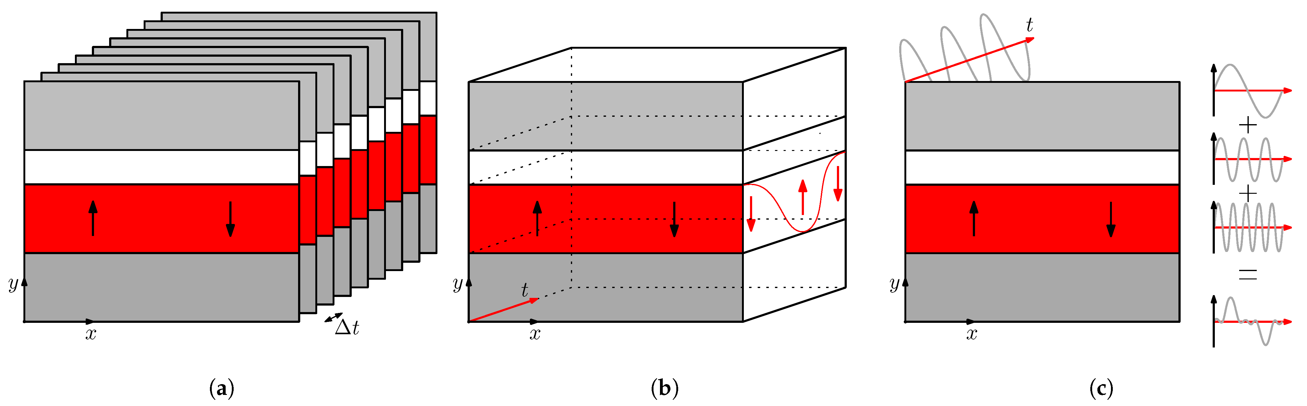
First, the framework of isogeometric analysis is introduced. The B-spline basis functions are defined for their use in geometry and solution discretization. The variational formulations of the magnetic problems are introduced including the Newton–Raphson method for taking the nonlinear material characteristics into account. The principle of three different dynamic solvers are detailed, i.e., the time-stepping technique, the space-time Galerkin approach, and the harmonic balance method, as exemplified in Figure 1. They constitute respectively: discrete, continuous, and modal time-discretizations of the dynamic motional eddy-current problem, which can be seen as 2.5D, 3D, and 2D methods, for the considered slotless and slotted benchmarks in 2D space, where 2.5D refers to a temporal sequence of 2D spatial simulations, 3D relies on a complete discretization of the space-time cylinder, and 2D only necessitates to resolve Fourier coefficients for reconstructing the time-harmonic evolution.
2.1. Isogeometric Analysis
The isogeometric analysis provides a powerful framework for the spatial discretization of partial differential equations (PDEs) arising in physics, such as solid mechanics, fluid dynamics, or electromagnetics [8]. Piecewise polynomials, B-splines, are considered as basis functions for the solution of the PDEs as well as for shape and geometry discretization. This class of numerical method integrates both mesh and polynomial degree refinements, which are useful to resolve geometrical and physical singularities as well as local features. The advantages compared to the traditional finite element method are an exact geometrical description and a smooth solution due to the higher continuity of the basis functions.
To build the B-splines basis functions, one starts to define an increasing sequence of points in to form a knot vector:
following Cox–de-Boor’s identity [9], where n is the number of B-spline functions and p is the degree of the polynomial, each knot has the multiplicity . When the knots are equally spaced, the knot vector is called uniform; otherwise, it is non-uniform. The multiplicity counts the number of times a knot is repeated in the vector. When the multiplicity of a knot is exactly , the basis function is continuous or interpolatory at that knot. For an open knot vector, the starting and last knots (0 and 1) are repeated times. In general, basis functions are continuous at a knot . Starting from piecewise constant functions of degree :
B-splines of higher-order can be defined recursively [9] as:
B-splines are naturally extended in any dimension d, by means of the tensor product between d univariate B-splines:
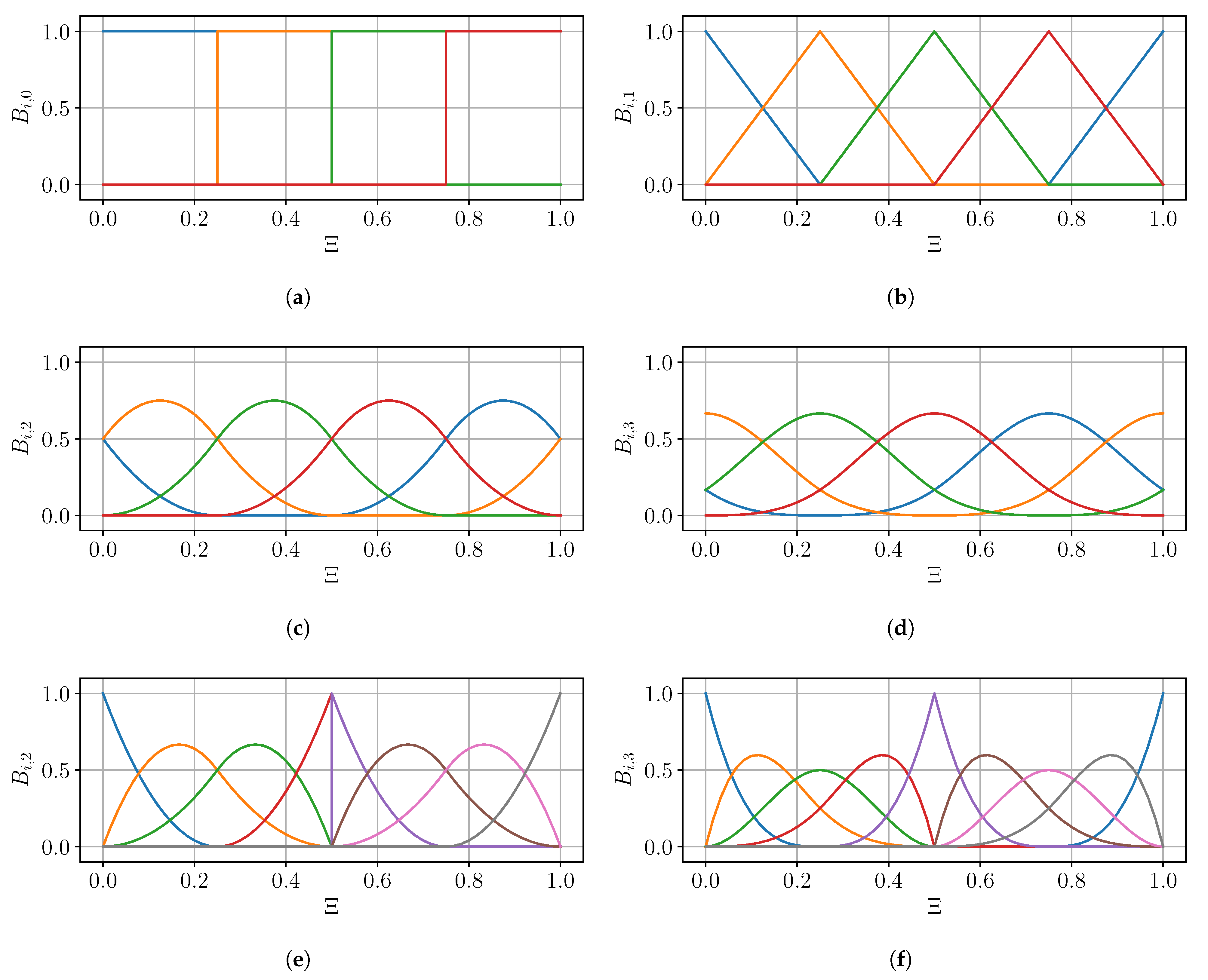
Periodic B-splines of increasing degree are shown in Figure 2a–d for a uniform knot vector. Correspondingly, periodic B-splines for a nonuniform knot vector, i.e., where the multiplicity is controlled, are shown in Figure 2e–f. B-splines can be extended to more complex functions, such as non-uniform rational B-splines (NURBS) as well as truncated hierarchical B-splines or THB-splines. NURBS are useful to represent conics and are commonly used in computer-aided design (CAD) models to represent industrial parts. NURBS are obtained by appending weights to each B-spline basis function. THB-splines enable residual-based adaptive refinements to be performed [10]. Furthermore, they offer a drastic reduction of the number of degrees of freedom (dofs) and reduced support.
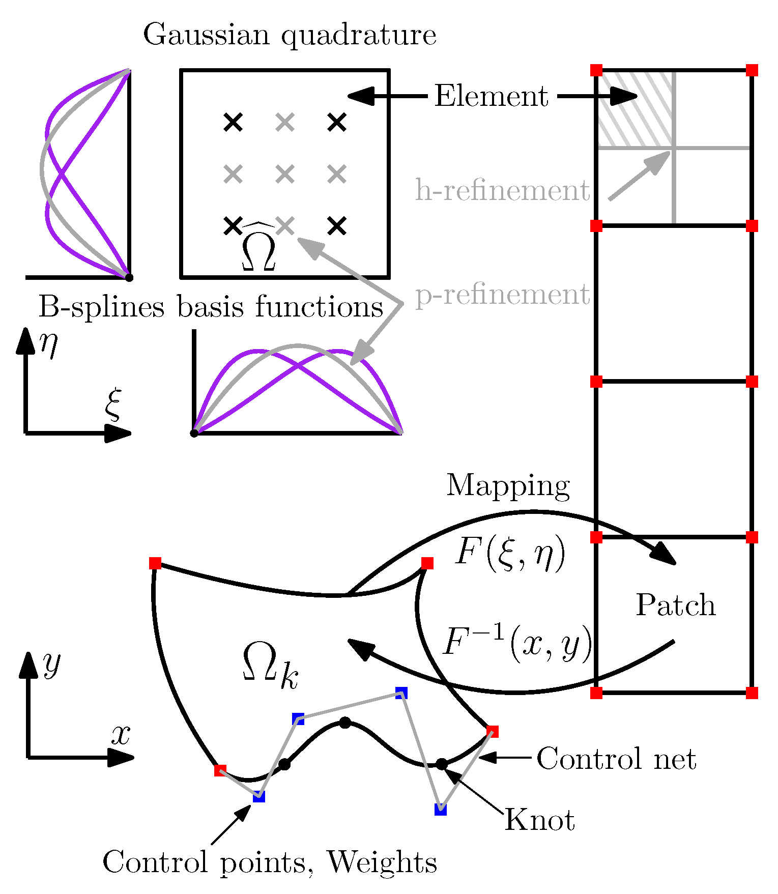
The geometry has to be discretized to be IGA-compatible. Several approaches are possible depending on the shapes, complexity of the model, and the numerical implementation. Since the tensor product construction is most often employed with IGA, the reference element is , where d is the dimension. In most electromagnetic applications, different materials interact within the same domain; therefore, discontinuous material properties and sources arise. The geometry can exhibit either nonconforming or conforming interfaces. The latter is preferred as it yields simpler formulations. Either the single patch or multipatch approach is possible. The single patch approach refines the knot vector and increases the knot multiplicities to decrease the level of continuity at the generated interfaces. The multipatch approach simply glues multiple elements with a given continuity at the interfaces, most often or . The multipatch approach based on NURBS offers a flexible description of the shapes of the interfaces between patches. A schematic of a multipatch discretization with IGA is represented in Figure 3. The parametrizations are indicated, which map each patch of the physical domain to the reference element or computational domain . Algebraic methods are used for the parametrization; in particular, Coon’s patch approach [11] is used for assembling surface patches from their boundary curves. However, other methods can be applied, such as PDE-based methods, and methods based on convex quadratic cost functional minimization [12,13]. For geometries with nonmatching boundaries, different techniques exist, such as Mortar methods [14], or discontinuous Galerkin methods (DG) [15].
A spline curve is defined as a linear combination of B-splines defined in (3) and control points:
where are the control points exemplified by colored squares in Figure 3. The control net is the gird formed by the piecewise linear curves that link all the control points. Additional weights can be introduced to form NURBS basis functions. Similarly, B-splines or NURBS parametrizations of multivariate geometries are created through a tensor product of univariate curves, leading to the creation of surfaces, manifolds, and volumes. Different algorithms have been conceived to produce refinements, transformations, and deformations of these structures [8,9,16]. h-refinement is obtained through knot insertion and is exemplified in Figure 3, p-refinement through degree elevation, and k-refinement is a degree elevation followed by knot insertion. Transformations include translations, rotations, and scalings. Concerning deformations, modifications of coordinates, and weights of the control points are possible. The coordinates can be either 3D Cartesian or 4D homogeneous coordinates if the weights are included.
2.2. Spatial Discretization of Nonlinear Magnetic Problems
Considering first a magnetostatic problem in the plane, it follows that B = and the magnetic vector potential = is reduced to a scalar field. In 2D, is obviously independent of z, and therefore = 0 falls naturally. Taking as the magnetic permeability, as the imposed electrical current density in the coil regions and as the remanent magnetic flux density of the permanent magnets, the strong form in 2D is a Laplace problem that reads:
The discrete solution approximation of the PDE is obtained with the Galerkin method. The isoparametric approach is chosen, meaning that the same approximation space is taken as the scalar Hilbert space:
which is a subset of the bivariate B-spline grad-conforming basis functions that vanish on the Dirichlet boundary , for both the test and trial functions. The variational formulation of the boundary value problem reads: Find , such that:
The solution is written as a linear combination of general B-spline basis functions , which span the approximation space , such that :
The bilinear operator for assembling the stiffness matrix entries and the inner product for assembling the right-hand side are given by:
where is the 2D curl operator, which corresponds to a 90-degree clockwise rotation of the gradient. In 2D Cartesian, . In practice, for implementation purposes, the curl can be obtained using the product between the Levi–Civita symbol and the field gradient. In 2D, this antisymmetric matrix reads:
The entries for the right-hand side given by the integral of a general function f are approximated numerically. The function f is tested against the basis function and is replaced by a Gaussian quadrature on elements partitioning the domain :
where, for each element, are the weights for the quadrature points of position . The quadrature is done in the physical domain, using the appropriate mapping , its Jacobian, and the chain rule for composed functions. The essential boundary conditions are imposed weakly through a lifting and projection [17].
To include the effect of the nonlinear constitutive equations, i.e., the nonlinear soft-magnetic material B-H characteristics, two methods are usually considered: the fixed-point method (FPM) or the Newton–Raphson method (NRM). A comparison between both nonlinear methods is presented in [18] in the various frameworks of the isogeometric analysis, the finite element method, and the spectral element method. In this paper, the NRM is considered to account for the field dependency of the magnetic permeability , using the Jacobian matrix J. The solution is updated at each iteration with the increment . Optionally, is a relaxation parameter chosen such that is a minimum. In practice, this is achieved through a line search algorithm [19]. The considered isotropic Newton–Raphson formulation can be written as:
and is implemented through its tensor form:
Different methods exist for discretizing the time dimension. In Maxwell’s equations describing low-frequency eddy current problems, a first-order time derivative is present, which yields a parabolic problem. To discretize the time gradient, different approximation methods are possible and are categorized into two classes: discrete and continuous. Continuous methods, such as the space-time Galerkin method, are detailed in Section 2.5. Discrete methods are referred to as time-stepping techniques, which constitute the subject of the next section.
2.3. Time-Stepping Technique
The most common time-stepping techniques are the so-called -methods [1]. The general algebraic system is considered:
where M and S are the mass and stiffness matrices, respectively, while b is the source term. The discrete time series is introduced:
where is the time step. The matrix R is introduced as:
Thus, the first-order ordinary differential equation reads:
Finite difference discretization of the time derivative is introduced using two levels, so that the -scheme reads:
where is the implicitness parameter, which can generate some of the implicit and explicit time-stepping schemes presented in Table 1. An explicit scheme is only a function of the previous time steps, while an implicit scheme is a function of previous and current time steps.
The precision indicated in Table 1 refers to the error made at a specific time t, and is different from the local truncation error, which is defined as the error made in one step, indicated in (28)–(31):
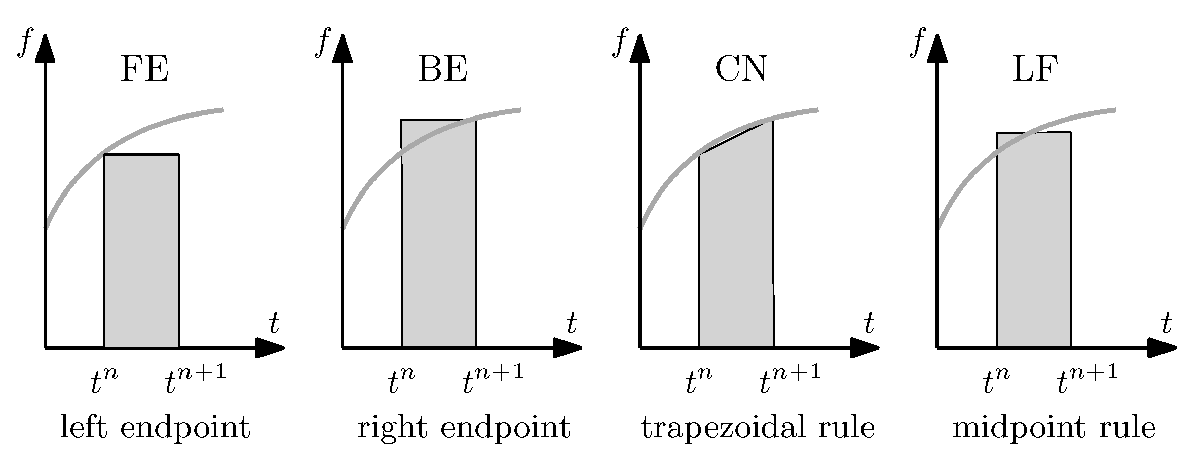
The -schemes introduced in (28)–(31) use different numerical time-integration quadrature rules, which are graphically exemplified in Figure 4 [20]. Explicit schemes have a low computational cost per time step and are simple to implement as well as to parallelize. However, small time-step values are required for stability reasons, especially for high speeds and high mesh-size aspect ratios. Implicit schemes exhibit stability over a wider range of time steps and do constitute a good iterative solver for steady-state problems. However, they have a higher cost per time step and are more difficult to implement as well as parallelize. They may get insufficiently accurate for unsteady transient problems as the time steps increases, which deteriorates the convergence [20]. More advanced transient solvers have been proposed, such as the three-level explicit leap-frog method, or fractional-step -methods. As the two-level methods can only be at most second-order accurate, higher-order time integration methods have been developed, such as the Adams methods and the Runge–Kutta methods [21].
An alternative to discrete time-stepping approaches consists of using continuous methods instead. After the high-order Galerkin methods have been applied in space, it is only natural to extend these methods to the space-time manifold. For instance, the space-time Galerkin isogeometric methods, which are truly 4D methods, have been presented [2,3] for single and multiple space-time patches.
In practice, each application has different requirements in space and in time. The optimal basis functions are the ones that directly embed the characteristic properties of the signal in their core. In the space domain, this is done with mimetic or structure-preserving basis functions, which have been introduced already for Maxwell’s problems [22]. In the time domain, few situations can arise in electrical machine applications with permanent magnet arrays.
Steady-state operations often appear in periodical systems evolving at a constant speed, such as rotating machines or long-stroke linear machines with many repeating geometrical periods, which yield fields with a discrete and finite frequency spectrum. The best basis functions in time might, therefore, be trigonometric functions, i.e., the Fourier series. Solving the problems in terms of the coefficients of these series is commonly referred to as the harmonic balance (HB) method [4,5].
2.4. Harmonic Balance Method
The harmonic balance (HB) method is a powerful alternative to a transient solver when the time-periodic steady-state solution is sought. Moreover, it yields very good efficiency when the time-harmonic content is small, i.e., when the time signals are reasonably smooth. The application of the HB method is mainly restricted to discrete and small frequency spectrum applications, although the considered frequencies can be widely spaced. Indeed, it is not uncommon that the highest frequency is orders of magnitude higher than the lowest frequency. This would require an enormous amount of time-stepping in practice and lead to prohibitive integration cost [23]. Originally, the HB method was employed for solving nonlinear electrical circuits, analog RF, and microwave problems in the frequency domain. The response and total harmonic distortion (THD) of a system under single or multi-tone excitation can be analyzed efficiently using the HB method. Frequency sweeping can efficiently simulate the performance of a system for a wide range of operating points. Outside of electromagnetic applications, the HB method has been applied to flow problems [24], mechanical vibrations, and deformations [25].
The harmonic balance has been extended to finite element applications, especially transformer problems, where the electric circuit coupling with magnetics is important. It has been applied to both and formulations [26,27] and compared with time-periodic finite element (TPFEM) approaches. Thanks to this method, the influence of the DC bias [28], due to cosmic radiation [29] for instance, on the losses can be studied more efficiently. The HB method has been applied to shielding and welding problems [30], laminated cores [31], and induction heating [32]. Multiphysics simulations for microelectromechanical systems (MEMS) using the HB method have been proposed [33]. Electrical machines with linear material characteristics have been modeled in 2D [34,35]. However, the HB method has not yet been applied to nonlinear motional eddy current problems. Furthermore, the convergence of the HB method has not yet been clearly demonstrated in the literature.
The idea of the harmonic balance method is to expand the time dimension of the fields into truncated time-harmonic series:
with the relationship . In the rest of this section, the spatial dependency is frequently omitted from the notation. The Fourier transform is applied to the nonlinear diffusion equation:
In between each nonlinear iteration, the time signals are reconstructed from the Fourier coefficients, the nonlinear relationship is applied on the time signal , before being transformed back to the frequency domain. The harmonic balance is therefore an alternating time-frequency scheme, which solves for the Fourier coefficients and alleviates time-stepping stability issues.
For solving the fully-coupled real-valued scheme, starting from (33) and using the real Fourier transform yields:
where the derivative matrix D is given by:
The matrix M only represents the sources due to the permanent magnet array as the system (35) is solved using the Newton–Raphson method. The term is obtained at each node through:
This illustrates the alternating time-frequency approach of the harmonic balance method.
It is possible to decouple the system of equations of the HB method [36]. The complex-valued problem derived from the decoupled harmonic balance is linearized using the fixed-point method, as described in [37]. The decoupled approach is well suited for situations where magnetic cross-coupling is not too critical. However, in general, the accuracy and robustness of the decoupled approach can be limited. Therefore, the fully coupled approach should be considered for general cases, in order to observe and analyze the convergence, before simplifying the system further. The solving scheme has to be adapted depending on whether a complex or real-valued Fourier series expansion is considered. If the Newton iterations are considered, it is beneficial to use the real Fourier transform. Indeed, the bilinear operator is real, and, therefore, differentiable. This is not straightforward for the complex-valued operator [38,39], for which the construction of the Jacobian matrix is cumbersome. Instead, for the complex-valued operator, a fixed-point method (FPM) is often preferred [18,37,40].
Depending on the selected scheme and the size of the system, different solvers can be used. For fully coupled harmonic balance, with large system size and wide frequency spectrum, iterative solvers [41], such as GMRES [42] or QMR [30], can be employed with appropriate block preconditioners and smoothers. This can also be resolved with multigrid (MG) solvers [39], which propagate the information from a fine mesh to a coarser mesh, where the matrix is inverted directly, and the information is transferred back to the finer space. They can be algebraic (AMG) [43], geometric (GMG), or geometric agglomerated algebraic multigrid solvers (GAMG) [44]. Geometric multigrid approaches are natural in the context of isogeometric analysis and can be either of type p-MG [45] or h-MG [46]. For the decoupled harmonic balance approach [37,40], the only coupling mechanism present is through the equivalent source terms on the right-hand side; therefore, each harmonic is solved separately and sequentially, for which a direct solver can be used. Direct solvers can also be used to solve the fully coupled harmonic balance if relatively small systems with limited frequency content are considered, which is the case in the numerical experiments presented in this work.
A few simplifications of the scheme can be made, depending on the type of excitation and source. If the source is composed of odd harmonics, then only odd harmonics are required for the solution and its derivatives [39]. Therefore, even harmonics are removed from the unknown solution vector, since they are identically null. In the case of purely complex-valued sinusoidal time excitation, only one frequency is needed to represent the signal, while, for a real-valued sinusoidal signal, the spectrum consists of two frequencies, which are conjugate symmetric, i.e., Hermitian. In this case, it is possible to replace the discrete Fourier transform (DFT) with a discrete cosine transform (DCT), thereby reducing the size of the system by a factor 2. Further harmonic reduction can be realized if a priori or a posteriori knowledge about the harmonic content is available [47].
It might be necessary to have a certain constraint on the mesh, depending on the number of harmonics considered. In the periodic motional problems considered in this paper, the time dimension is closely related to the first geometrical dimension x, along which the uniform translation is operated. Therefore, it can be beneficial to impose sufficient mesh refinement for resolving the highest frequency component considered in the HB scheme.
In order to include the motion within the harmonic balance framework, different techniques can be applied depending on the motion profile and the geometry. Depending on whether the eddy currents are only of interest in the stator or the mover, the Eulerian or Lagrangian approaches can be used, respectively. However, if the eddy currents in both mover and stator are important, or if both stator and mover present a complex topology, a coupling strategy in the airgap should be considered [6]. The considered applications focus on surface-mounted permanent magnet electrical machines, and the eddy currents are solely of interest in the stator, notably, no electrical conductivity is considered in the mover. The considered motion profiles are exclusively constant displacement speeds in both linear and rotating coordinate systems. Therefore, the geometry and the relative motion of the permanent magnet array can be both approximated by a periodic traveling magnetization wave, without the need for a coupling strategy. In particular, only the fundamental time-harmonic can be considered as the basis for the moving spatial-magnetization function:
The square wave representing the spatial distribution of the magnetization in the direction of motion can be approximated by means of Fourier series. However, in practice, only the fundamental spatial-harmonic is considered by employing the following simple source term in the permanent magnet array region:
The exact description of the actual magnetization spatial distribution is not crucial if the eddy currents are only of interest in the stator because the airgap acts as a low-pass filter and tends to exhibit a sinusoidal magnetic flux density distribution. The proposed approach allows for incorporating easily the motion of a surface-mounted permanent magnet array in the frequency domain without stator–mover coupling. Furthermore, it enables to study efficiently the eddy current phenomena in complex stator core geometries and with nonlinear B-H characteristics, as will be demonstrated numerically in Section 3.
2.5. Space-Time Galerkin Approach
The space-time Galerkin approach consists of extruding the geometrical model along the additional time dimension. The spline basis functions are then built on the entire domain. Specific augmented Levi–Civita symbols are used to assemble the curl and time-derivative operators, from the overall space-time gradient. For a 2D geometrical model, discretized with a scalar-valued magnetic vector potential:
where and , is the 2D Levi–Civita symbol defined in (13), and is the Kronecker symbol. The advantage of this method is that it enables to guarantee the smoothness of the solution, as well as to perform the advantageous features of IGA, such as the adaptive mesh refinements, in both space and time. The computational cost, however, is impaired, since the problem exhibits an additional dimension. Therefore, many more degrees of freedom have to be solved simultaneously, as opposed to sequentially, using the traditional time-stepping techniques.
2.6. Benchmarks
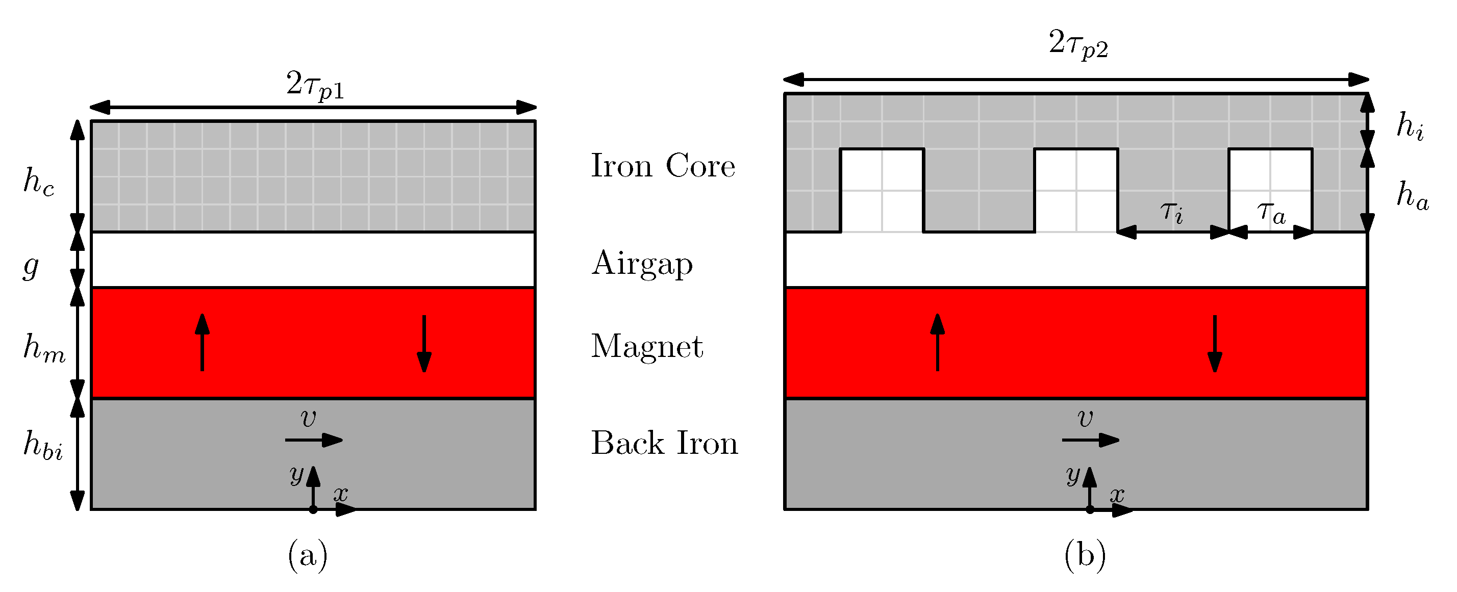
The two considered 2D benchmark geometries are shown in Figure 5, and their respective dimensions are gathered in Table 2. In the first benchmark, the core region is slotless, while the second benchmark is slotted. This is done to demonstrate that both the correct force-ripple profiles and the mean damping force can be accurately predicted. Furthermore, such slotless and slotted geometries constitute the most common topologies in linear permanent magnet machine applications. The Dirichlet boundary conditions are imposed at both the top and bottom boundaries, while periodic conditions link each side. Both the iron and core regions have nonlinear magnetic properties corresponding to the material M270-50A-50Hz [48]. The radial magnet array has a relative magnetic permeability of and a remanent magnetic flux density of T. To force the soft-magnetic materials to strongly saturate, the value of the remanent magnetic flux density is artificially increased by 40 %. Only the stator core region is electrically conductive with S/m. The depth of the domain is taken as mm. The permanent magnet array is translated with constant linear speeds m/s.
3. Results
3.1. Slotless Benchmark
For the slotless benchmark, the reference discretization is taken to be four elements along the height and 16 elements along the width per region as shown in Figure 5. The modeling environment consists of the Nutils FEM toolbox [49]. Bivariate splines of degree three are considered as basis functions, which are periodic along the x-direction, as shown in Figure 2b. Odd harmonics until , which is equivalently denoted as , are simulated for the harmonic balance. Three periods are simulated with 120 time steps per period for the transient time-stepping solver, which is a backward Euler solver with . The number of samples of the discrete Fourier transform is selected to be equivalent to the number of time-steps per period for the time-stepping solver, in order to match the resolution. Reducing the number of time-samples decreases the computational effort, for both the time-stepping approach and the harmonic balance solver.
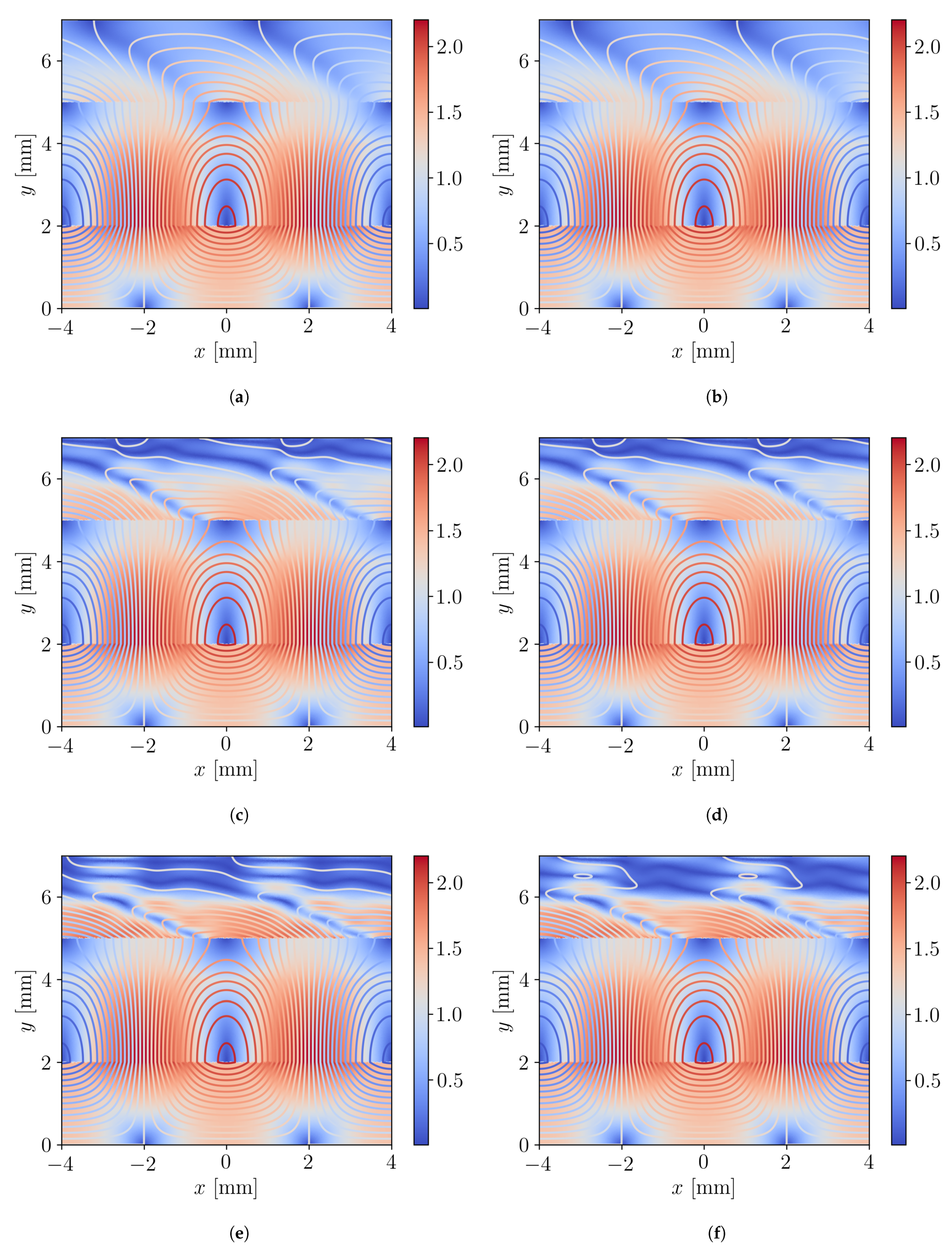
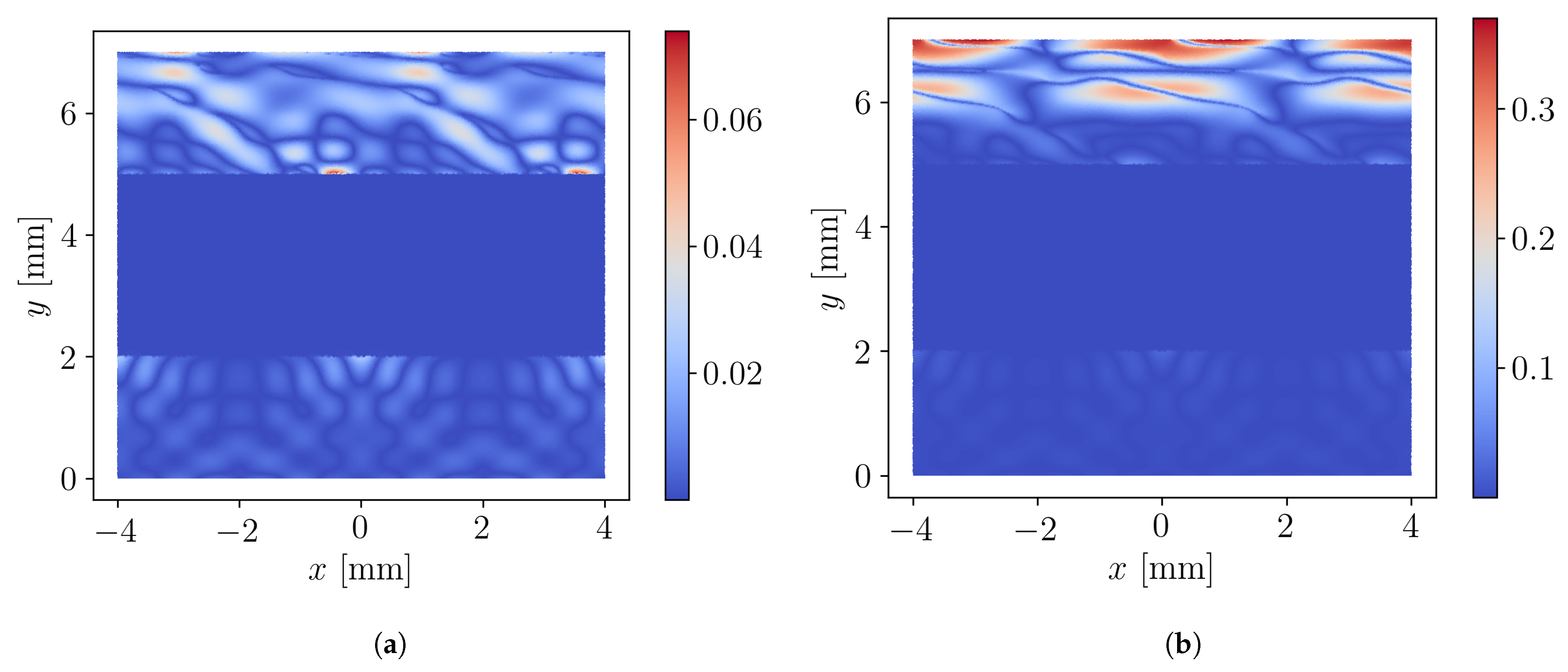
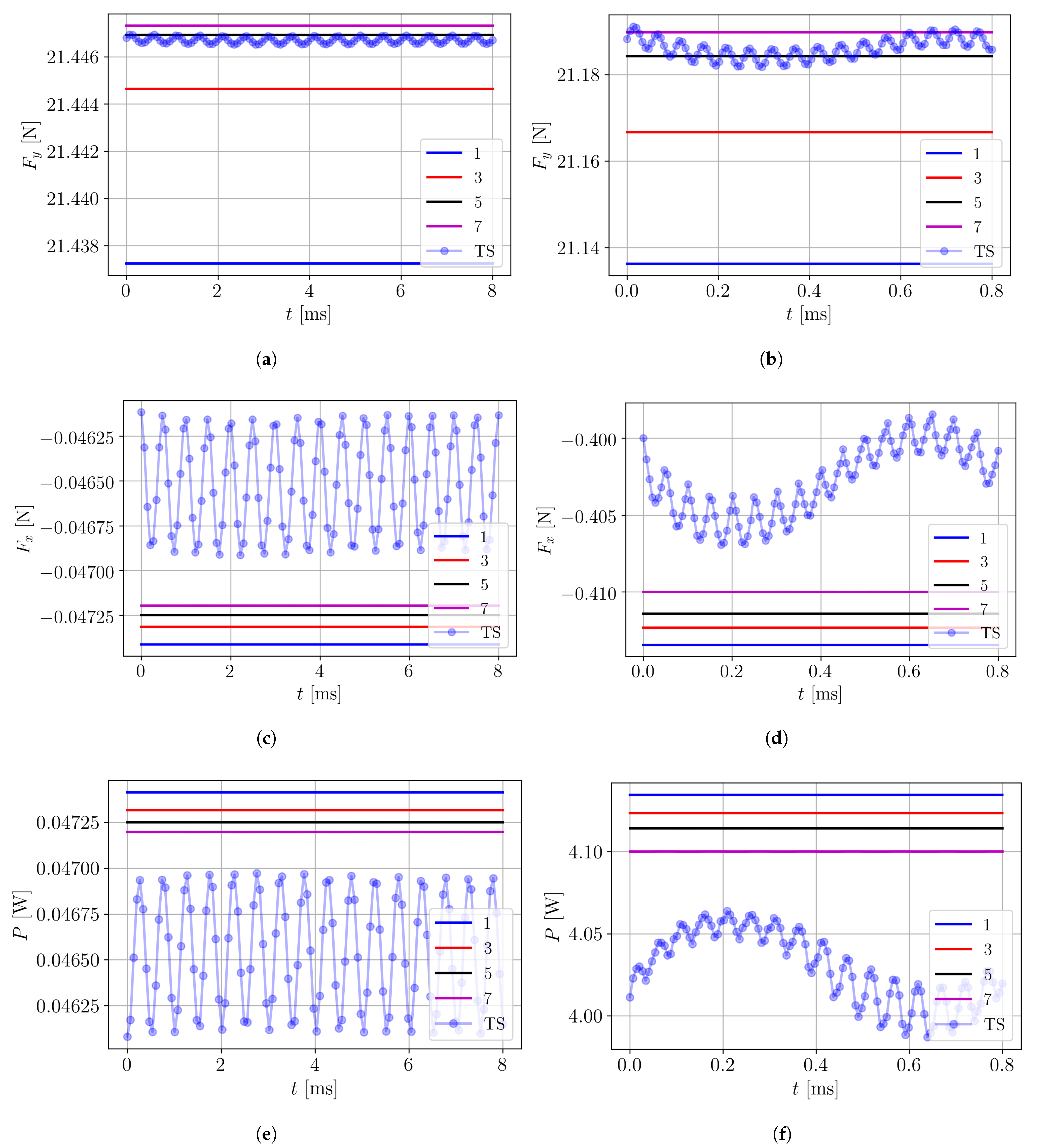
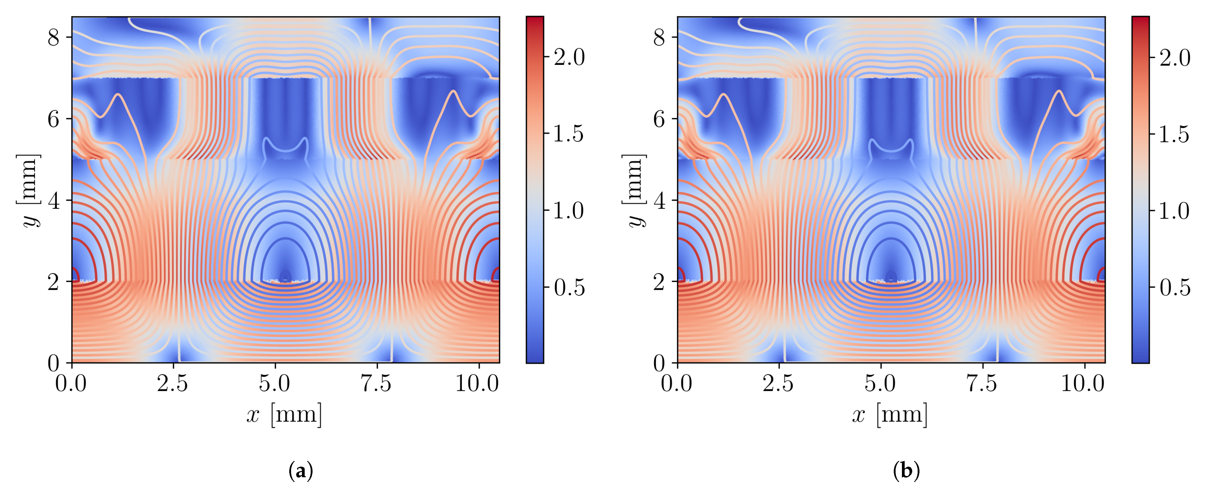
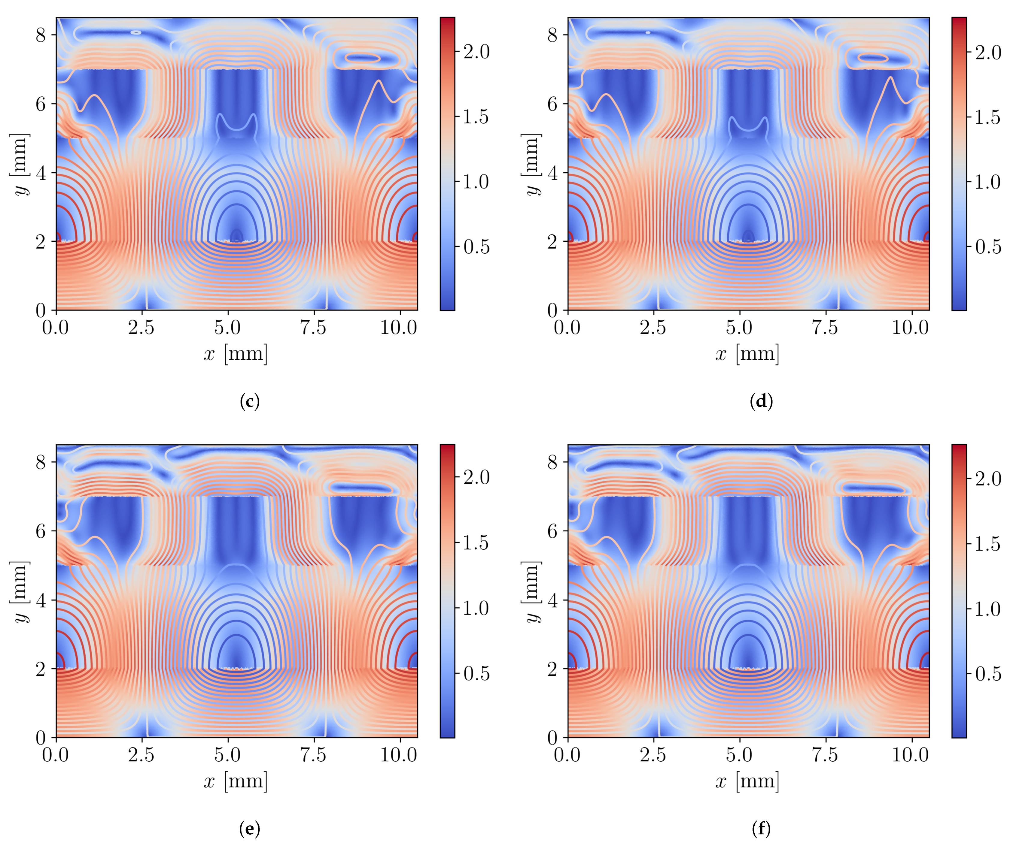
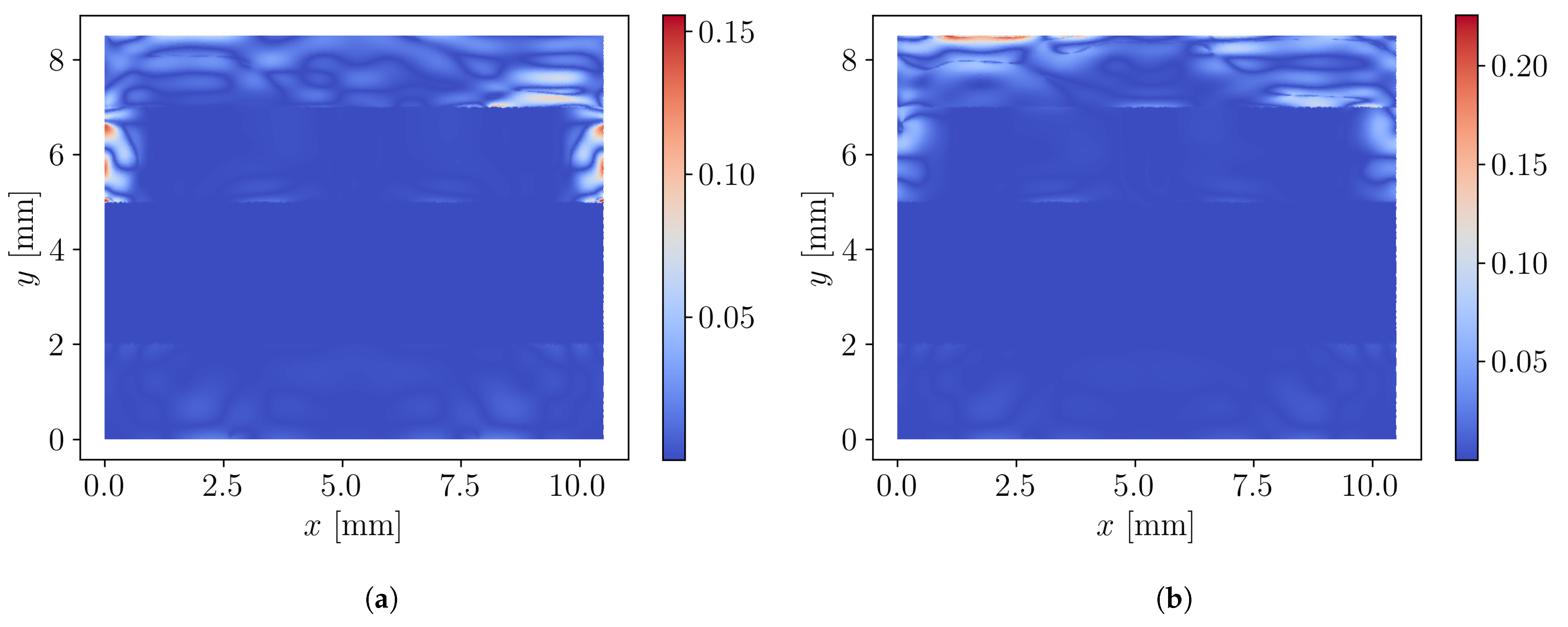
The magnetic flux density distributions for speeds m/s are shown for both the harmonic balance (HB) and time-stepping (TS) solvers in Figure 6. The distributions are matching very well at low speeds, while at 10 m/s the time-stepping approach suffers from small instabilities. The absolute value of the difference in magnetic flux density between both approaches is shown in Figure 7. A maximum discrepancy of 58 mT and 375 mT is found for speeds equal to 1 m/s and 10 m/s, respectively. The profiles of the attraction force, the damping force, and the eddy current losses in the core regions are shown for three different speeds in Figure 8, for an increasing number of considered harmonics. A good agreement is obtained between both solvers, with less than 2% discrepancy among the mean values of the times profiles, as shown in Table 3.
This discrepancy can be lowered by increasing the refinement in space and time, but the current discretization represents a trade-off between accuracy and computational effort. However, such a discrepancy is considered sufficiently accurate for the engineering problems considered in this work, where a discrepancy of 5 to 10% is typically accepted.
In this slotless core example, concerning Figure 8, completely flat profiles are expected, i.e., the amplitude of the ripples should tend to zero. This can be achieved using intensive h-refinements with the time-stepping approach, where the amplitude tends to the computer precision at the cost of an increased computational effort. Alternatively, with the HB method, the correct profiles are directly obtained at a reduced cost. The computational effort can be further reduced by relaxing the h-refinement and restricting the number of harmonics considered. The harmonic balance method has the advantage of being stable disregarding the considered speed, whereas the time-stepping approach gets unstable at high speeds, as shown on the distribution of Figure 6f and the profiles of Figure 8b,d,f, where unphysical spurious oscillations appear for m/s. As shown in Table 3, the force discrepancies increase by one order of magnitude for 10 m/s as compared to 1 m/s.
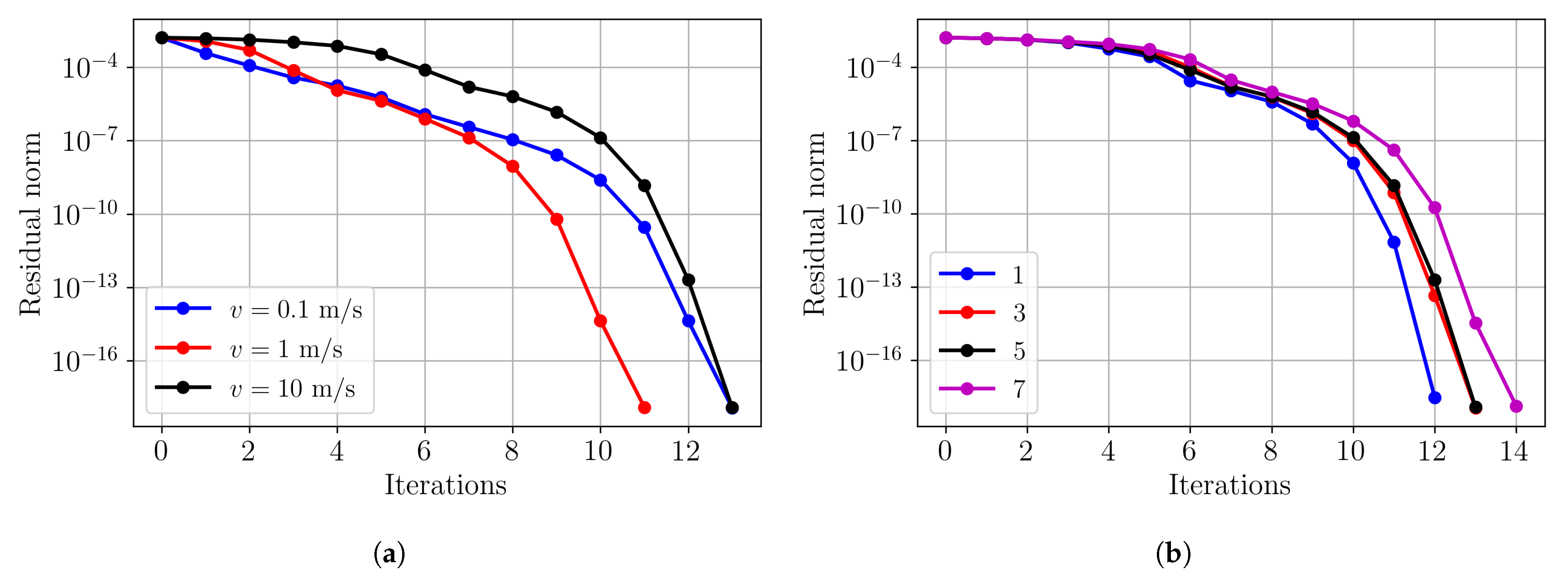
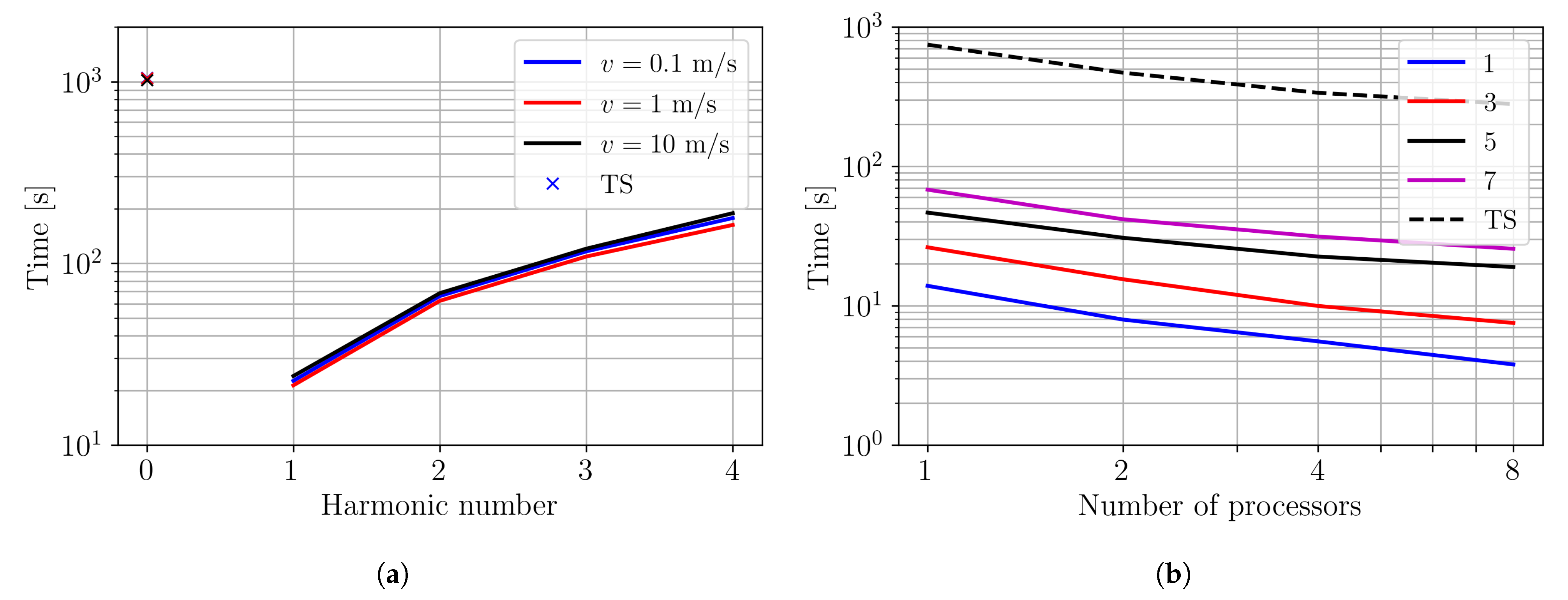
The nonlinear convergence of the solution is shown in Figure 9a for different speeds. The nonlinear convergence at a speed of 10 m/s for different considered harmonic spectra is shown in Figure 9b. The number of nonlinear iterations is reasonable and only slightly affected by the additional harmonic content. It indicates that the additional harmonic content has little effects on the final solution, which is also visible in Figure 8. The computational effort as a function of the number of considered harmonics is given in Figure 10a. The computational effort for the time-stepping approach is indicated at harmonic index zero as a reference. In this resistive eddy current regime, the computational effort of the time-stepping approach is independent of the displacement speed. Furthermore, the scaling of computational effort is shown in Figure 10b as the number of cores working in parallel for the matrix assembly is increased. It can be seen that the computational effort does not correspond between Figure 9b and Figure 10b for the case with one processor. The reason is that Figure 10b is obtained with a Linux machine, which enables the multithreading of the solving step, and therefore reduces the overall computational time. Depending on the number of considered harmonics, the proposed HB method achieves a speed up of at least a factor 11 compared to the time-stepping approach.
3.2. Slotted Benchmark
Similarly, for the slotted benchmark, the reference discretization is taken to be two elements along the height and two elements along the width per region as shown in Figure 5, with bivariates splines of degree 3. Odd harmonics until , or equivalently , are solved for the harmonic balance, and three periods are simulated with 120 time steps per period for the transient time-stepping solver.
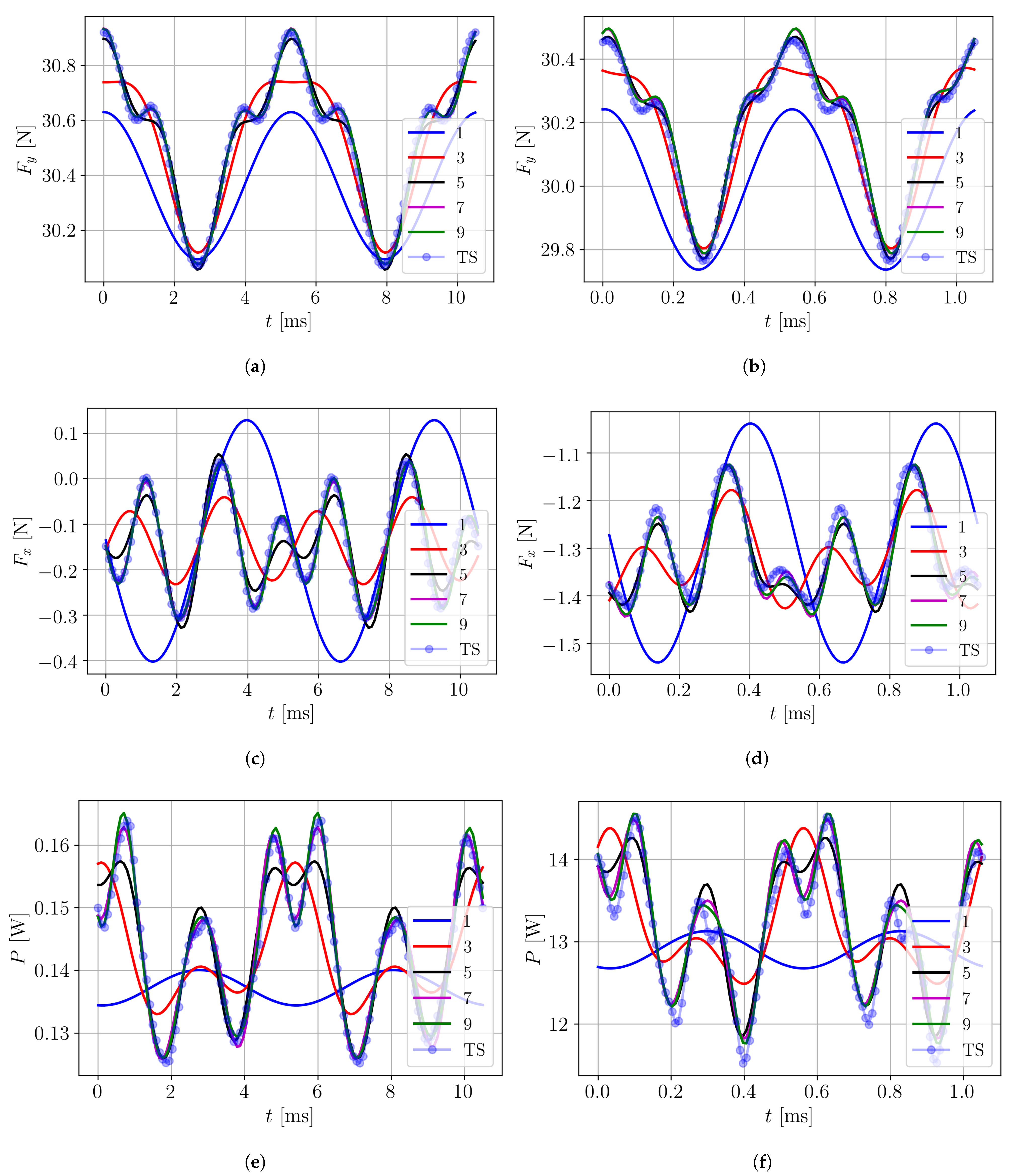
The magnetic flux density distributions are shown in Figure 11 for three different speeds. A very good agreement is observed between the time-stepping approach and the proposed harmonic balance approach. The absolute value of the difference in magnetic flux density between both approaches is shown in Figure 12. A maximum discrepancy of 138 mT and 213 mT is found for speeds equal to 1 m/s and 10 m/s, respectively. The profiles of the attraction force, the damping force, and the eddy current losses in the core regions are shown for two different speeds in Figure 13, for an increasing number of considered harmonics. In the slotted benchmark, the cogging profiles shown in Figure 13 are correctly predicted from . For a speed of 10 m/s, the discrepancy between the mean values of the three post-processed parameters is less than 1%, as can be seen in Table 4. Furthermore, the mean deviation, calculated as the normalized root-mean-square (rms) error, is less than 2% for all profiles.
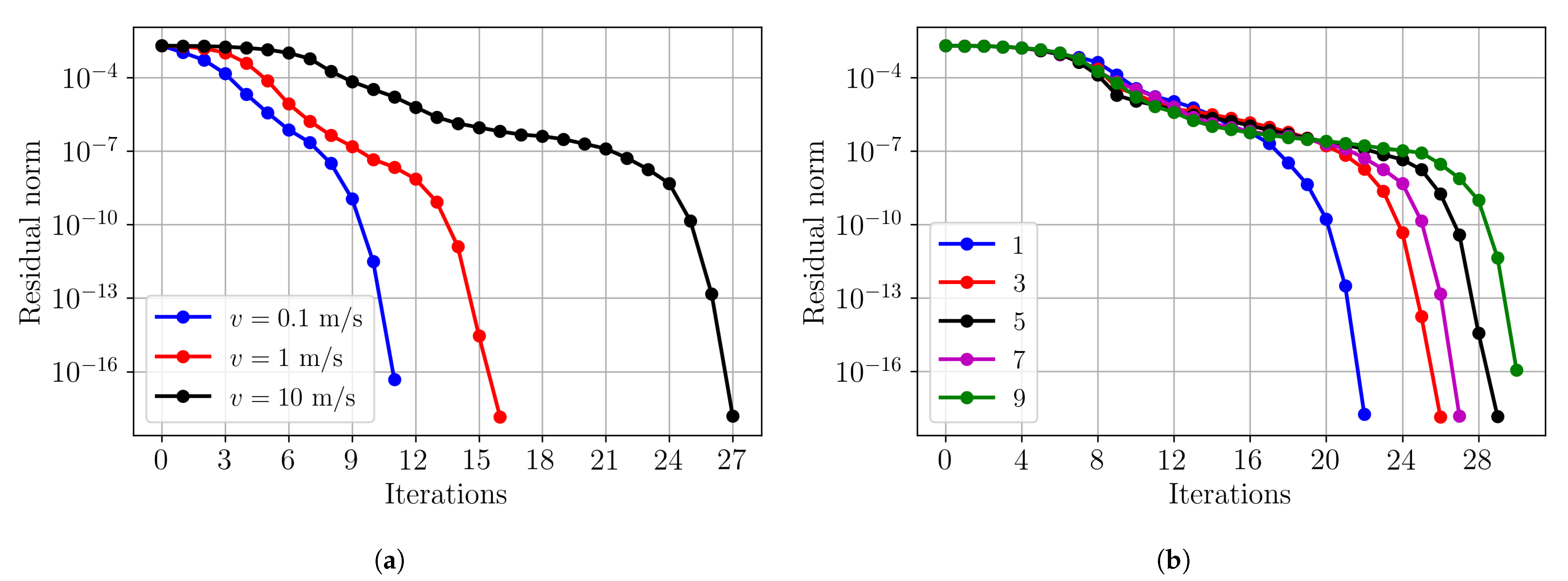
The nonlinear convergence of the solution is shown in Figure 14a for different speeds. It is observed that the number of iterations increases significantly for increasing speeds in the slotted example, as compared to the slotless example (Figure 9a). Indeed, the higher-order harmonics are truly excited by the slotting effect. Furthermore, for a speed of 10 m/s, the nonlinear convergence for different harmonic spectra considered in the HB method is given in Figure 14b, which demonstrates a large increase in iterations as compared to the slotless case in Figure 9b.
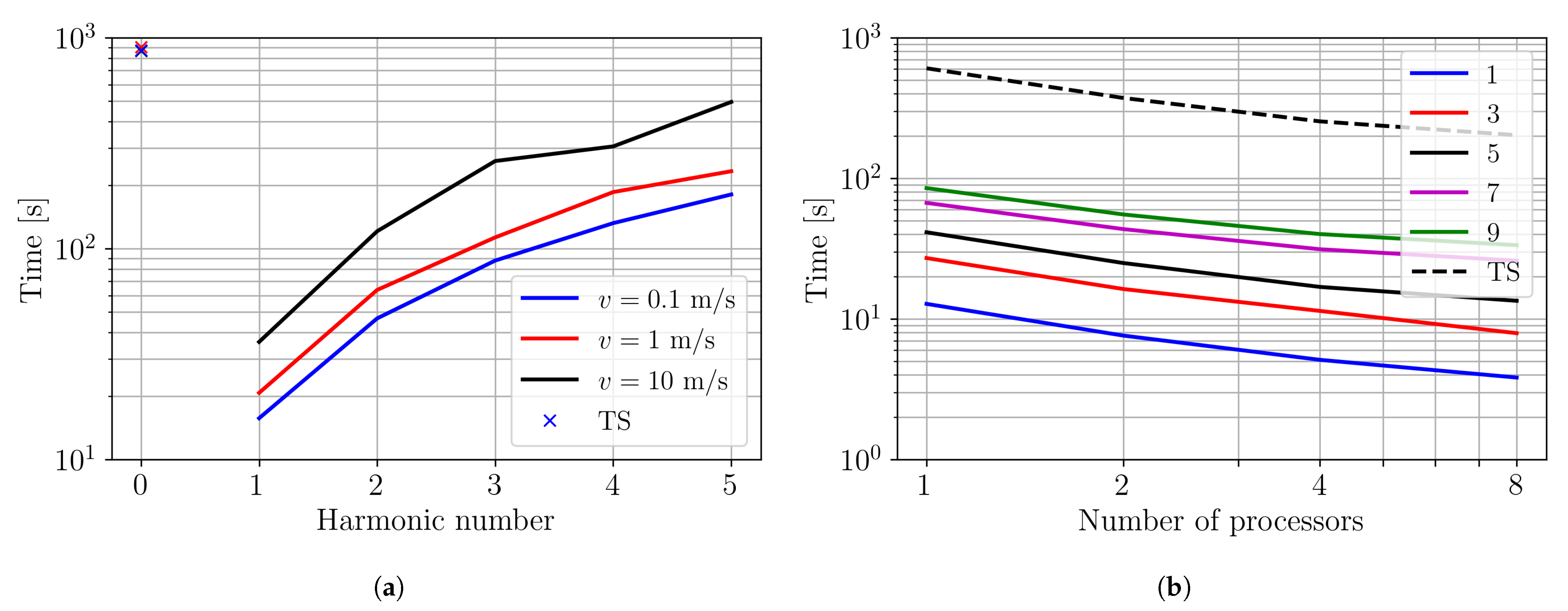
The computational effort as a function of the number of considered harmonics is given in Figure 15a. The computational effort for the time-stepping approach is indicated at harmonic index zero as a reference. In this resistive eddy current regime, the computational effort of the time-stepping approach is independent of the displacement speed. The scaling of computational effort is shown in Figure 15b as the number of cores working in parallel for the matrix assembly is increased. Depending on the number of considered harmonics, the proposed HB method achieves a speed up of at least a factor 7 compared to the time-stepping approach.
3.3. Comparison with the Space-Time Approach
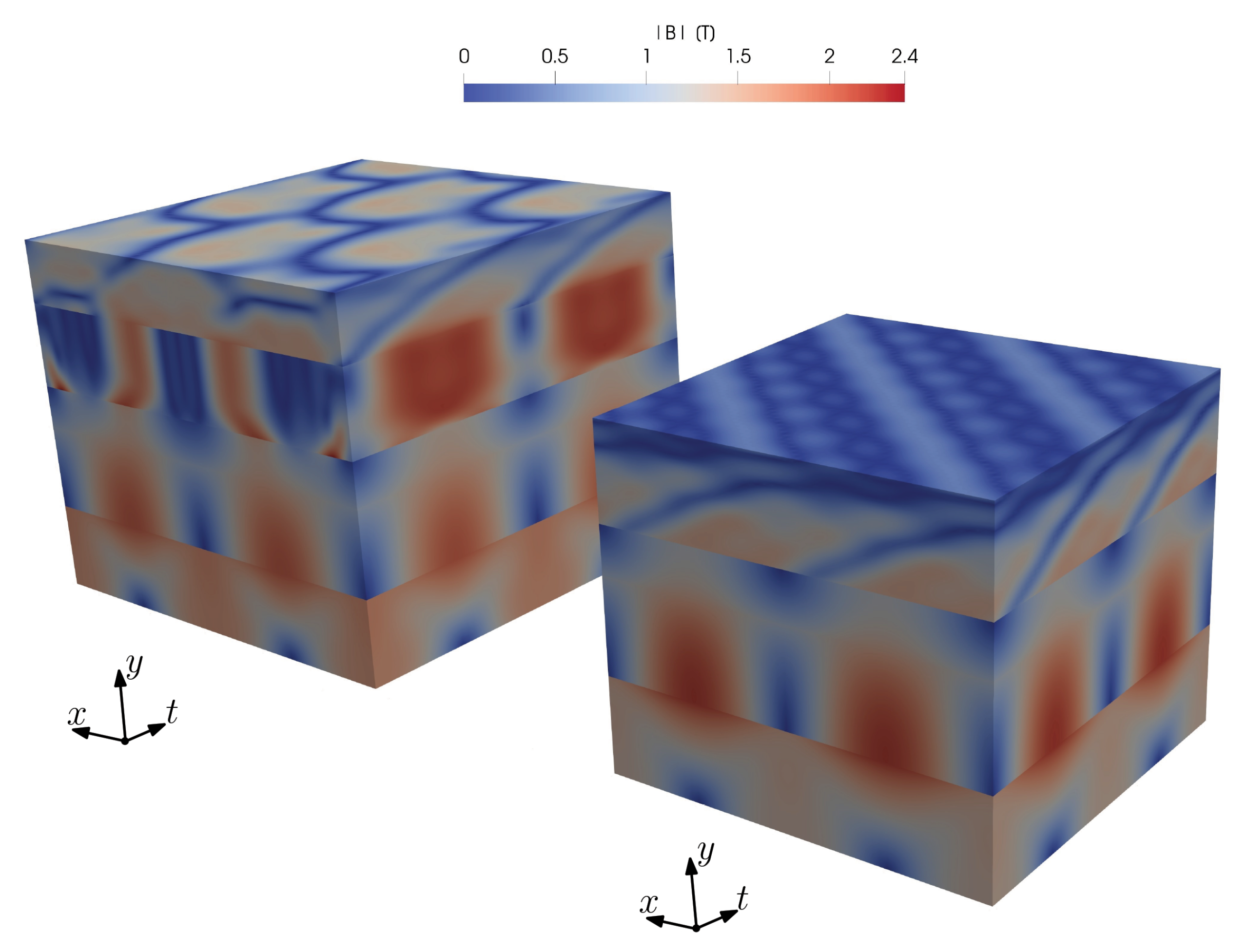
The solutions obtained with the space-time Galerkin approach are given as the distribution of the modulus of the magnetic flux density in Figure 16 for both the slotted and slotless benchmarks. The direction of motion can be seen from the top plane in the slotless example.
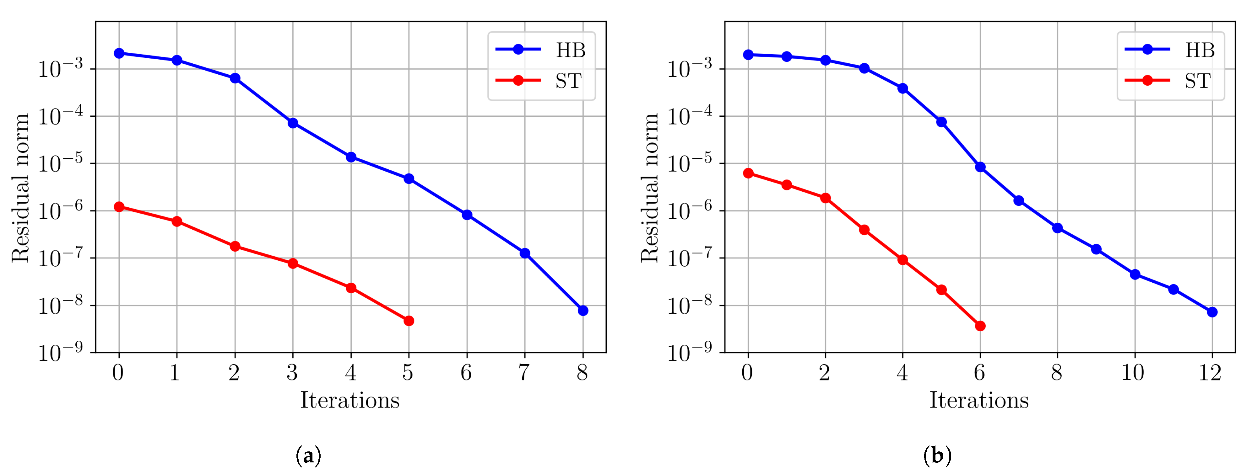
Figure 17 shows the nonlinear convergence of the space-time and harmonic balance approaches. Since the harmonic balance is based on trigonometric basis functions, as the time signals get more complex, more harmonics are necessary, which degrades the convergence due to cross-coupling effects. For the slotless benchmark, 5 and 8 iterations are necessary to reach convergence for the space-time and harmonic balance approaches, respectively, while it takes 6 and 12 iterations for the slotted problem to converge. As expected, the number of iterations needed for the space-time solver is much less sensitive to the complexity of the solution in time than for the HB solver. However, since an HB iteration is typically faster than an ST iteration due to reduced dimensionality, the harmonic balance approach is still competitive overall.
In Table 5, the computational effort for the slotless and slotted benchmarks are given, for the space-time CG approach illustrated in Figure 1a, and compared to the harmonic balance method, and the time-stepping technique. The temporal and spatial discretizations described in Section 3.1 are reused for both the slotless and slotted benchmarks. The only difference is that only eight elements along the periodic x-direction are used for the slotless benchmark. Because of the correlation between the x and time t dimensions due to the motion, eight elements are taken along the periodic time dimension as well. A Newton–Raphson tolerance of is specified for all solvers, and a speed of 1 m/s is considered.
The results of Table 5 demonstrate that the space-time approach is advantageous compared to the time-stepping technique, with a speedup factor of 6. Furthermore, they show that the harmonic balance method is the most efficient solution overall, with a speedup factor of 34 and 10 compared to the time-stepping technique for the slotless and slotted benchmarks, respectively. However, as the solution gets more complex in terms of local features and as the time-harmonic content is increased, i.e., from solution including up to the third and seventh time harmonics, the advantages of the harmonic balance method are lessened.
3.4. Refinement Strategy
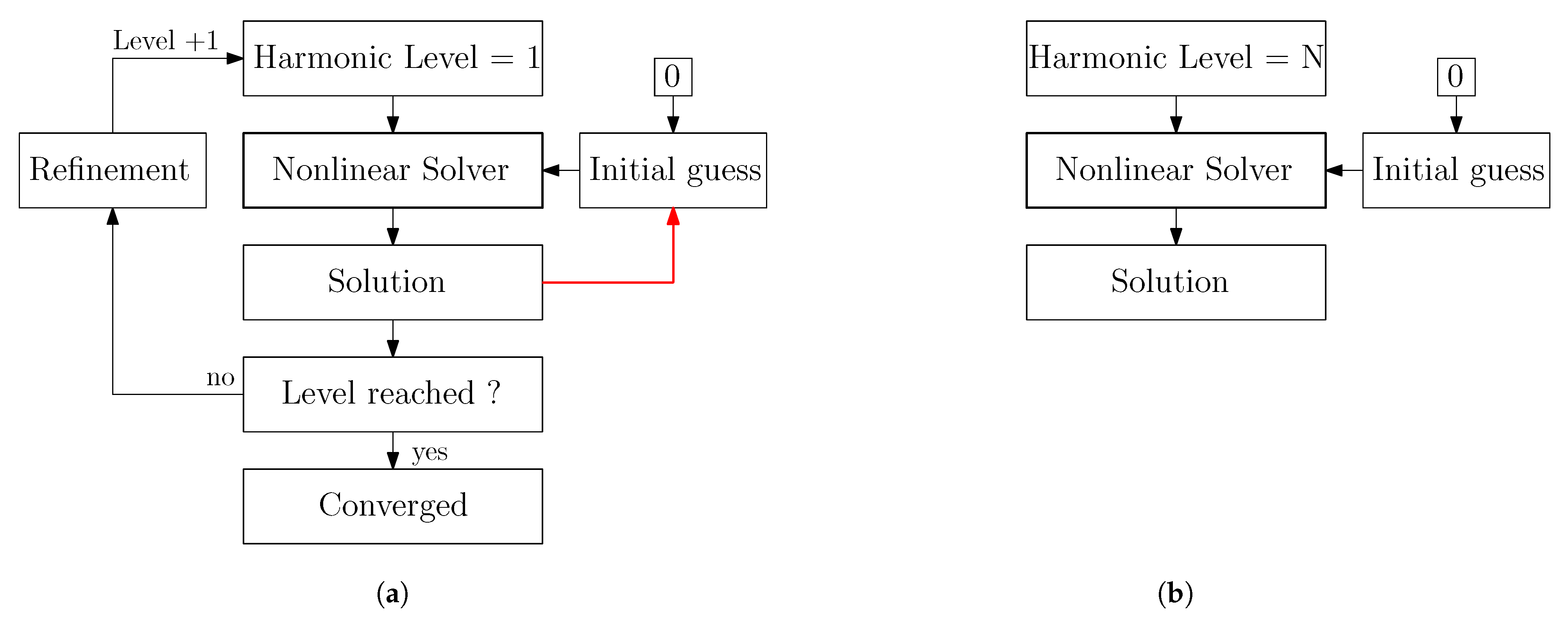
When solving large problems using the harmonic balance solver, for instance with significant harmonic spectra and/or in three dimensions, the computational efficiency can be impaired. One way to speed up the overall solving time is to adopt a progressive harmonic refinement strategy. This strategy is called progressive as opposed to adaptive, since the refinement is not based on error estimators. It is illustrated in Figure 18a, as opposed to the traditional approach depicted in Figure 18b. Instead, the system is first solved using the fundamental harmonic alone and this intermediate solution is then used as an initial guess for the next Newton–Raphson iteration, which solves the system for incrementally richer harmonic content. For instance, applying this progressive harmonic refinement strategy to the slotted benchmark can save up to 37% of the computational time reported in Table 5, which uses the traditional approach. This use of this progressive harmonic refinement strategy can become mandatory to avoid convergence plateau, as visible in Figure 17b, when the magnetic saturation is more pronounced and especially on larger problem sizes. Otherwise, it might be challenging to guarantee the convergence of the nonlinear solver.
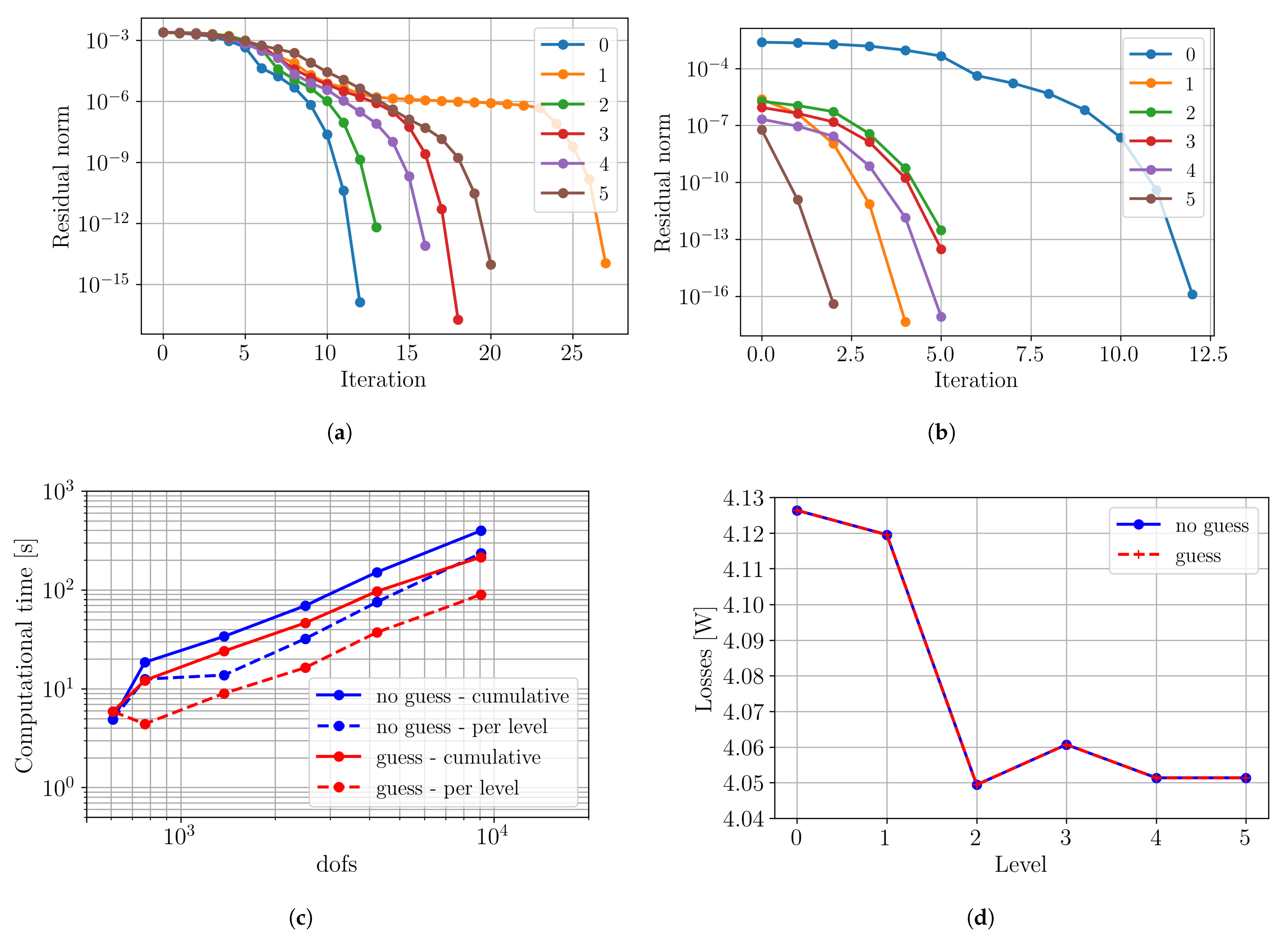
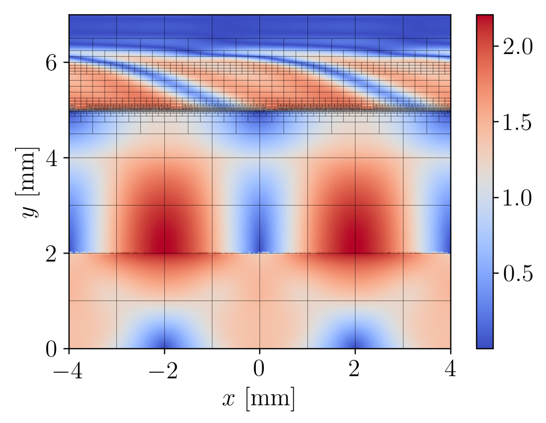
A similar idea of the progressive harmonic refinement strategy can be applied to adaptive mesh refinements [10], independently of the time-discretization method being used. By replacing harmonic level by mesh level in the schematic of Figure 17, the corresponding scheme can be obtained, realized using the projection of the solution at the previous mesh level to the refined mesh. The effects of this strategy are exemplified in Figure 19. Figure 19a,b show that the number of nonlinear iterations is greatly reduced. Moreover, the possible convergence plateau is avoided. Altogether, it reduces the computational effort as shown in Figure 19c. The reduction is such that the cumulative time of the proposed strategy can get smaller than the original time at one level, as seen at levels 1 and 5. Furthermore, Figure 19d demonstrates that both strategies converge to the same value, which verifies that the initial guess strategy does not stir towards a wrong solution. The resulting magnetic flux density distribution including the adaptively-refined mesh discretization is shown in Figure 20. It can be seen that the refinements are concentrated next to the core interface, where the stronger eddy currents are concentrated.
4. Conclusions
The harmonic balance approach for simulating nonlinear motional eddy current problems is presented in this paper. It is demonstrated that the proposed approach is well suited for the simulation of nonlinear motional eddy current problems. Furthermore, it is more computationally efficient than the backward Euler time-stepping approach for reaching the steady-state solution. In addition, it prevents from having to choose a time step value, which influences the convergence and final values by introducing numerical oscillations.
Slotless and slotted benchmarks are simulated to establish the accuracy of the time profiles of post-processed parameters, as well as to verify that the cogging waveform is correctly predicted. The mean discrepancies and average deviations are less than 2% for all cases. The magnetic flux density modulus distributions are compared between both approaches. A good agreement is obtained on the field distributions. Maximum discrepancies of 58 mT and 375 mT for the slotless benchmark, as well as 138 mT and 213 mT for the slotted benchmark, at speeds of 1 m/s and 10 m/s, respectively, are registered. These discrepancies occur in regions away from the main field and may be attributed in majority to the time-stepping solver instabilities. For the considered refinements at high speeds, e.g., 10 m/s, the harmonic balance solver has demonstrated better stability and an absence of numerical oscillations on the time profiles, compared to the time-steeping approach. Moreover, the convergence of the norm of the residual is demonstrated for the proposed harmonic balance method. Depending on the number of considered harmonics, the computational time is reduced by at least a factor of 7 and 11 compared to the time-stepping approach, for the slotted and slotless benchmark, respectively.
The space-time Galerkin approach has been detailed and compared to the harmonic balance and time-stepping approaches on both the slotless and slotted benchmarks. It is shown that the harmonic balance is the most advantageous method for the considered nonlinear motional eddy current problems.
Finally, spatial adaptive refinements are implemented for the harmonic balance method together with an initial guess for the Newton–Raphson iterations based on the solution at the previous level, which enables a faster convergence. On the slotless benchmark, it results in a decrease in the computational effort by a factor 2. Progressive harmonic refinements are proposed, which improve the convergence properties. On the slotted benchmark, this refinement strategy improves the computational efficiency by 37%. These strategies are also important to guarantee convergence for larger and more complex three-dimensional problems.
Funding
This research received no external funding.
Acknowledgments
The author would like to thank Joost van Zwieten for his help in the implementation of the numerical methods in the Nutils library [49].
Conflicts of Interest
The author declares no conflict of interest.
Abbreviations
The following abbreviations are used in this manuscript:
| 1D, 2D, 3D, 4D | One-, Two-, Three-, Four-dimensional |
| 2.5D | Two and a half dimensional |
| BE | Backward Euler |
| B-spline | Basis spline |
| CAD | Computer-Aided Design |
| CG | Continuous Galerkin |
| CK | Crank–Nicolson |
| DC | Direct Current |
| dofs | degrees of freedom |
| DCT | Discrete Cosine Transform |
| DFT | Discrete Fourier Transform |
| DG | Discontinuous Galerkin |
| FEM | Finite Element Method |
| FE | Forward Euler |
| FPM | Fixed-Point Method |
| GAMG | Geometric Algebraic Multigrid |
| GMG | Geometric Multigrid |
| GMRES | Generalized Minimal Residual |
| HB | Harmonic Balance |
| IGA | Isogeometric Analysis |
| LF | Leapfrog |
| MEMS | Microelectromechanical Systems |
| MG | Multigrid |
| NRM | Newton–Raphson Method |
| NURBS | Non-Uniform Rational B-splines |
| PDEs | Partial Differential Equations |
| QMR | Quasi-Minimal Residual |
| RF | Radio Frequency |
| rms | Root Mean Square |
| ST | Space-Time |
| THB-spline | Truncated Hierarchical B-spline |
| THD | Total Harmonic Distortion |
| TP | Time-Periodic |
| TS | Time-Stepping |
References
- Quarteroni, A.; Quarteroni, S. Numerical Models for Differential Problems; Springer: Milan, Italy, 2009. [Google Scholar]
- Loli, G.; Montardini, M.; Sangalli, G.; Tani, M. Space-time Galerkin isogeometric method and efficient solver for parabolic problem. arXiv preprint 2019, arXiv:1909.07309. [Google Scholar] [CrossRef]
- Hofer, C.; Langer, U.; Neumüller, M.; Toulopoulos, I. Time-multipatch discontinuous Galerkin space-time isogeometric analysis of parabolic evolution problems. Verlag Österreichischen Akademie Wissenschaften 2018. [Google Scholar] [CrossRef] [Green Version]
- Yamada, S.; Bessho, K.; Lu, J. Harmonic balance finite element method applied to nonlinear AC magnetic analysis. IEEE Trans. Magn. 1989, 25, 2971–2973. [Google Scholar] [CrossRef]
- Yamada, S.; Biringer, P.; Bessho, K. Calculation of nonlinear eddy-current problems by the harmonic balance finite element method. IEEE Trans. Magn. 1991, 27, 4122–4125. [Google Scholar] [CrossRef]
- De Gersem, H.; Gyselinck, J.; Dular, P.; Hameyer, K.; Weiland, T. Comparison of sliding-surface and moving-band techniques in frequency-domain finite-element models of rotating machines. COMPEL Int. J. Comput. Math. Electr. Electron. Eng. 2004. [Google Scholar] [CrossRef]
- Demenko, A.; Hameyer, K.; Nowak, L.; Zawirski, K.; De Gersem, H.; Ion, M.; Wilke, M.; Weiland, T. Trigonometric interpolation at sliding surfaces and in moving bands of electrical machine models. COMPEL- Int. J. Comput. Math. Electr. Electron. Eng. 2006. [Google Scholar] [CrossRef]
- Hughes, T.J.R.; Cottrell, J.A.; Bazilevs, Y. Isogeometric analysis: CAD, finite elements, NURBS, exact geometry and mesh refinement. Comput. Methods Appl. Mech. Eng. 2005, 194, 4135–4195. [Google Scholar] [CrossRef] [Green Version]
- De Boor, C. A Practical Guide to Splines; Applied Mathematical Sciences; Springer: New York, NY, USA, 1978; Volume 27. [Google Scholar]
- Friedrich, L.A.J.; Roes, M.G.L.; Gysen, B.L.J.; Lomonova, E.A. Adaptive isogeometric analysis applied to an electromagnetic actuator. IEEE Trans. Magn. 2019, 55, 1–4. [Google Scholar] [CrossRef] [Green Version]
- Farin, G.; Hansford, D. Discrete Coons patches. Comput. Aided Geom. Des. 1999, 16, 691–700. [Google Scholar] [CrossRef]
- Hinz, J.; Möller, M.; Vuik, C. Elliptic grid generation techniques in the framework of isogeometric analysis applications. Comput. Aided Geom. Des. 2018, 65, 48–75. [Google Scholar] [CrossRef] [Green Version]
- Hinz, J.; Abdelmalik, M.; Möller, M. Goal-Oriented Adaptive THB-Spline Schemes for PDE-Based Planar Parameterization. arXiv 2020, arXiv:2001.08874. [Google Scholar]
- Buffa, A.; Corno, J.; de Falco, C.; Schöps, S.; Vázquez, R. Isogeometric Mortar Coupling for Electromagnetic Problems. SIAM J. Sci. Comput. 2020, 42, B80–B104. [Google Scholar] [CrossRef] [Green Version]
- Buffa, A.; Perugia, I. Discontinuous Galerkin approximation of the Maxwell eigenproblem. SIAM J. Numer. Anal. 2006, 44, 2198–2226. [Google Scholar] [CrossRef]
- Piegl, L.; Tiller, W. The NURBS Book; Springer Science & Business Media: Berlin/Heidelberg, Germany, 2012. [Google Scholar]
- Vázquez, R. A new design for the implementation of isogeometric analysis in Octave and Matlab: GeoPDEs 3.0. Comput. Math. Appl. 2016, 72, 523–554. [Google Scholar] [CrossRef]
- Friedrich, L.A.J.; Curti, M.; Gysen, B.L.J.; Lomonova, E.A. High-order methods applied to nonlinear magnetostatic problems. Math. Comput. Appl. 2019, 24, 19. [Google Scholar] [CrossRef] [Green Version]
- Ramière, I.; Helfer, T. Iterative residual-based vector methods to accelerate fixed point iterations. Comput. Math. Appl. 2015, 70, 2210–2226. [Google Scholar] [CrossRef]
- Kuzmin, D. A Guide to Numerical Methods for Transport Equations; University Erlangen-Nuremberg: Erlangen, Germany, 2010. [Google Scholar]
- Gödel, N.; Schomann, S.; Warburton, T.; Clemens, M. GPU accelerated Adams–Bashforth multirate discontinuous Galerkin FEM simulation of high-frequency electromagnetic fields. IEEE Trans. Magn. 2010, 46, 2735–2738. [Google Scholar] [CrossRef]
- Palha, A.; Koren, B.; Felici, F. A mimetic spectral element solver for the Grad–Shafranov equation. J. Comput. Phys. 2016, 316, 63–93. [Google Scholar] [CrossRef] [Green Version]
- Agilent Technologies. Advanced Design System. In Harmonic Balance Simulation, User Guide; 2011. [Google Scholar]
- Cvijetić, G.; Gatin, I.; Vukčević, V.; Jasak, H. Harmonic Balance developments in OpenFOAM. Comput. Fluids 2018, 172, 632–643. [Google Scholar] [CrossRef]
- Weeger, O.; Wever, U.; Simeon, B. Isogeometric analysis of nonlinear Euler–Bernoulli beam vibrations. Nonlinear Dyn. 2013, 72, 813–835. [Google Scholar] [CrossRef] [Green Version]
- Plasser, R.; Koczka, G.; Bíró, O. A nonlinear magnetic circuit model for periodic eddy current problems using T,Φ-Φ formulation. COMPEL- Int. J. Comput. Math. Electr. Electron. Eng. 2017. [Google Scholar] [CrossRef]
- Plasser, R.; Takahashi, Y.; Koczka, G.; Bíró, O. Comparison of two methods for the finite element steady-state analysis of nonlinear 3D periodic eddy-current problems using the A,V-formulation. Int. J. Numer. Model. Electron. Netw. Devices Fields 2018, 31, e2279. [Google Scholar] [CrossRef]
- Plasser, R.; Koczka, G.; Bíró, O. Improvement of the Finite-Element Analysis of 3D, Nonlinear, Periodic Eddy Current Problems Involving Voltage-Driven Coils under DC Bias. IEEE Trans. Magn. 2017, 54, 1–4. [Google Scholar] [CrossRef]
- Zhao, X.; Guan, D.; Meng, F.; Zhong, Y.; Cheng, Z. Computation and Analysis of the DC-Biasing Magnetic Field by the Harmonic-Balanced Finite-Element Method. Int. J. Energy Power Eng. 2015, 5, 31. [Google Scholar] [CrossRef] [Green Version]
- Bachinger, F.; Langer, U.; Schöberl, J. Efficient solvers for nonlinear time-periodic eddy current problems. Comput. Vis. Sci. 2006, 9, 197–207. [Google Scholar] [CrossRef] [Green Version]
- Hollaus, K. A MSFEM to simulate the eddy current problem in laminated iron cores in 3D. COMPEL Int. J. Comput. Math. Electr. Electron. Eng. 2019, 38, 1667–1682. [Google Scholar] [CrossRef] [Green Version]
- Roppert, K.; Toth, F.; Kaltenbacher, M. Simulating induction heating processes using harmonic balance FEM. COMPEL Int. J. Comput. Math. Electr. Electron. Eng. 2019, 38, 1562–1574. [Google Scholar] [CrossRef]
- Halbach, A.; Geuzaine, C. Steady-state, nonlinear analysis of large arrays of electrically actuated micromembranes vibrating in a fluid. Eng. Comput. 2018, 34, 591–602. [Google Scholar] [CrossRef] [Green Version]
- Pries, J.; Hofmann, H. Harmonic balance FEA of synchronous machines using a traveling-wave airgap model. In Proceedings of the 2011 IEEE Vehicle Power and Propulsion Conference, Chicago, IL, USA, 6–9 September 2011; pp. 1–6. [Google Scholar]
- Wick, M.; Grabmaier, S.; Juettner, M.; Rucker, W. Motion in frequency domain for harmonic balance simulation of electrical machines. COMPEL- Int. J. Comput. Math. Electr. Electron. Eng. 2018, 37, 1449–1460. [Google Scholar] [CrossRef]
- Driesen, J.; Van Craenenbroeck, G.D.T.; Hameyer, K. Implementation of the harmonic balance FEM method for large-scale saturated electromagnetic devices. WIT Trans. Eng. Sci. 1999, 22, 10. [Google Scholar]
- Friedrich, L.A.J.; Gysen, B.L.J.; Lomonova, E.A. Modeling of integrated eddy current damping rings for a tubular electromagnetic suspension system. In Proceedings of the 12th International Symposium on Linear Drives for Industry Applications (LDIA), Neuchâtel, Switzerland, 1–3 July 2019; pp. 1–4. [Google Scholar]
- De Gersem, H.; Vande Sande, H.; Hameyer, K. Strong coupled multi-harmonic finite element simulation package. COMPEL Int. J. Comput. Math. Electr. Electron. Eng. 2001, 20, 535–546. [Google Scholar] [CrossRef]
- Bachinger, F. Multigrid Solvers for 3D Multiharmonic Nonlinear Magnetic Field Computations. Ph.D. Thesis, Johannes Kepler Universitat Linz, 2003. [Google Scholar]
- Friedrich, L.A.J.; Gysen, B.L.J.; Jansen, J.W.; Lomonova, E.A. Analysis of Motional Eddy Currents in the Slitted Stator Core of an Axial-Flux Permanent-Magnet Machine. IEEE Trans. Magn. 2020, 56, 1–4. [Google Scholar] [CrossRef] [Green Version]
- Saad, Y. Iterative Methods for Sparse Linear Systems; SIAM: Philadelphia, PA, USA, 2003. [Google Scholar]
- Pries, J.; Hofmann, H. Steady-state algorithms for nonlinear time-periodic magnetic diffusion problems using diagonally implicit Runge–Kutta methods. IEEE Trans. Magn. 2014, 51, 1–12. [Google Scholar] [CrossRef]
- Reitzinger, S.; Schöberl, J. An algebraic multigrid method for finite element discretizations with edge elements. Numer. Linear Algebra Appl. 2002, 9, 223–238. [Google Scholar] [CrossRef]
- OpenCFD Ltd. OpenFOAM: API Guide. Available online: www.openfoam.com (accessed on 7 January 2021).
- Tielen, R.; Möller, M.; Göddeke, D.; Vuik, C. Efficient p-multigrid methods for isogeometric analysis. arXiv 2019, arXiv:1901.01685. [Google Scholar]
- de Prenter, F.; Verhoosel, C.V.; van Brummelen, E.H.; Evans, J.A.; Messe, C.; Benzaken, J.; Maute, K. Scalable multigrid methods for immersed finite element methods and immersed isogeometric analysis. arXiv 2019, arXiv:1903.10977. [Google Scholar]
- Außerhofer, S.; Bíró, O.; Preis, K. An efficient harmonic balance method for nonlinear eddy-current problems. IEEE Trans. Magn. 2007, 43, 1229–1232. [Google Scholar] [CrossRef] [Green Version]
- Flux 12.2, User’s Guide and Material Library; 2016.
- van Zwieten, G.; van Zwieten, J.; Verhoosel, C.V.; Fonn, E.; van Opstal, T.; Hoitinga, W. Nutils (Version 7.0). Available online: www.nutils.org (accessed on 7 January 2021).
Figure 1.
Schematic representations of (a) the time-stepping technique, (b) the space-time approach, and (c) the harmonic balance method. The color code for the different regions is explained in Section 2.6.
Figure 1.
Schematic representations of (a) the time-stepping technique, (b) the space-time approach, and (c) the harmonic balance method. The color code for the different regions is explained in Section 2.6.

Figure 2.
B-spline basis of degree 0, 1, 2, 3 on an open uniform knot vector: (a) B-spline basis of degree 0, (b) B-spline basis of degree 1, (c) B-spline basis of degree 2, and (d) B-spline basis of degree 3. B-spline basis on an open nonuniform knot vector , (e) B-spline basis of degree 2, and (f) B-spline basis of degree 3.

Figure 3.
Conforming multipatch isogeometric discretization schematic.

Figure 4.
Graphical representation of the numerical integration rule on the interval for the -schemes (28)–(31).
Figure 4.
Graphical representation of the numerical integration rule on the interval for the -schemes (28)–(31).

Figure 5.
(a) Slotless and (b) slotted 2D benchmark geometries considered for validating the harmonic balance method.
Figure 5.
(a) Slotless and (b) slotted 2D benchmark geometries considered for validating the harmonic balance method.

Figure 6.
Magnetic flux density modulus distribution B in [T] and flux lines for the slotless benchmark at speed m/s, using the harmonic balance in (a,c,e), and the time-stepping approach in (b,d,f).
Figure 6.
Magnetic flux density modulus distribution B in [T] and flux lines for the slotless benchmark at speed m/s, using the harmonic balance in (a,c,e), and the time-stepping approach in (b,d,f).

Figure 7.
Absolute discrepancy in the magnetic flux density distribution in [T] between the harmonic balance and time-stepping solutions, (a) at 1 m/s and (b) at 10 m/s.
Figure 7.
Absolute discrepancy in the magnetic flux density distribution in [T] between the harmonic balance and time-stepping solutions, (a) at 1 m/s and (b) at 10 m/s.

Figure 8.
Attraction force , damping force , and eddy current losses P, for the slotless benchmark at speed m/s in (a,c,e) and m/s in (b,d,f), using the harmonic balance method with increasing number of harmonics and the time-stepping approach (TS).
Figure 8.
Attraction force , damping force , and eddy current losses P, for the slotless benchmark at speed m/s in (a,c,e) and m/s in (b,d,f), using the harmonic balance method with increasing number of harmonics and the time-stepping approach (TS).

Figure 9.
(a) Nonlinear convergence of the solution including up to the third harmonic, (b) nonlinear convergence at 10 m/s, for different harmonic spectra H.
Figure 9.
(a) Nonlinear convergence of the solution including up to the third harmonic, (b) nonlinear convergence at 10 m/s, for different harmonic spectra H.

Figure 10.
(a) Computational effort for the time-stepping approach (TS) and harmonic balance method with increasing harmonic content N and different speeds, (b) scaling of the computational effort by increasing the number of processors in parallel for the slotless benchmark.
Figure 10.
(a) Computational effort for the time-stepping approach (TS) and harmonic balance method with increasing harmonic content N and different speeds, (b) scaling of the computational effort by increasing the number of processors in parallel for the slotless benchmark.

Figure 11.
Magnetic flux density modulus distribution B in [T] and flux lines for the slotted benchmark at speed m/s, using the harmonic balance in (a,c,e), and the time-stepping approach in (b,d,f).
Figure 11.
Magnetic flux density modulus distribution B in [T] and flux lines for the slotted benchmark at speed m/s, using the harmonic balance in (a,c,e), and the time-stepping approach in (b,d,f).


Figure 12.
Absolute discrepancy in the magnetic flux density distribution in [T] between the harmonic balance and time-stepping solutions, (a) at 1 m/s and (b) at 10 m/s.
Figure 12.
Absolute discrepancy in the magnetic flux density distribution in [T] between the harmonic balance and time-stepping solutions, (a) at 1 m/s and (b) at 10 m/s.

Figure 13.
Attraction force , damping force , and eddy current losses P, for the slotted benchmark at speed m/s in (a,c,e) and m/s in (b,d,f), using the harmonic balance method with increasing number of harmonics and the transient approach.
Figure 13.
Attraction force , damping force , and eddy current losses P, for the slotted benchmark at speed m/s in (a,c,e) and m/s in (b,d,f), using the harmonic balance method with increasing number of harmonics and the transient approach.

Figure 14.
(a) Nonlinear convergence of the solution including up to the seventh harmonic, (b) nlinear convergence at 10 m/s, for different harmonic spectra H.
Figure 14.
(a) Nonlinear convergence of the solution including up to the seventh harmonic, (b) nlinear convergence at 10 m/s, for different harmonic spectra H.

Figure 15.
(a) Computational effort for the time-stepping approach (TS) and harmonic balance method with increasing harmonic content N and different speeds, (b) scaling of the computational effort by increasing the number of processors in parallel for the slotted benchmark.
Figure 15.
(a) Computational effort for the time-stepping approach (TS) and harmonic balance method with increasing harmonic content N and different speeds, (b) scaling of the computational effort by increasing the number of processors in parallel for the slotted benchmark.

Figure 16.
Space-time solutions for the slotted and slotless benchmarks of Figure 5, on the left and right, respectively.
Figure 16.
Space-time solutions for the slotted and slotless benchmarks of Figure 5, on the left and right, respectively.

Figure 17.
(a) Nonlinear convergence of the space-time approach and harmonic balance method with the third time harmonic for the slotless benchmark of Figure 5a, (b) nonlinear convergence of the space-time approach and harmonic balance method with the seventh time harmonic for the slotted benchmark of Figure 5b.

Figure 18.
Schematic representations of (a) the progressive harmonic refinement strategy, (b) the traditional approach.
Figure 18.
Schematic representations of (a) the progressive harmonic refinement strategy, (b) the traditional approach.

Figure 19.
(a) Residual norm at successive Newton–Raphson iterations for the untrimmed problem, increasing the refinement levels without initial guess and (b) with an initial guess obtained from the solution at the previous level; (c) evolution of the number of degrees of freedom and corresponding computational time; (d) convergence of the mean value of the eddy current losses for increasing refinement level.

Figure 20.
Magnetic flux density distribution B in [T] and mesh at the last level for the slotless benchmark.
Figure 20.
Magnetic flux density distribution B in [T] and mesh at the last level for the slotless benchmark.


Table 1.
-schemes for standard time-stepping approaches.
| Name | Scheme | Precision | |
|---|---|---|---|
| 0 | Forward Euler | explicit | |
| 0.5 | Crank–Nicolson | implicit | |
| 1 | Backward Euler | implicit |
Table 2.
Geometrical dimensions of the 2D benchmarks.
| Parameter | Value [mm] | Parameter | Value [mm] |
|---|---|---|---|
| 8.0 | 10.5 | ||
| 2.0 | 2.0 | ||
| g | 1.0 | 1.5 | |
| 2.0 | 1.5 | ||
| 2.0 | 2.0 |
Table 3.
Mean relative discrepancy in percentage, for the damping force , attraction force , and eddy current losses , between the transient time-stepping solution and the ones obtained with harmonic balance of increasing harmonic content N and upper harmonic order H, for speed m/s, for the slotless benchmark.
| [%] | [%] | [%] | |||||
|---|---|---|---|---|---|---|---|
| 1 m/s | 10 m/s | 1 m/s | 10 m/s | 1 m/s | 10 m/s | ||
| 1 | 1 | 4.41 × | 2.36 × 10 | ||||
| 2 | 3 | 9.63 × 10 | 9.20 × 10 | ||||
| 3 | 5 | 1.54 × 10 | 1.04 × 10 | 8.81 × 10 | |||
| 4 | 7 | 1.43 × 10 | 2.84 × 10 | 1.73 × 10 | |||
Table 4.
Mean and rms relative discrepancy in percentage, for the damping force , attraction force , and eddy current losses , between the transient time-stepping solution and the ones obtained with harmonic balance of increasing harmonic content N and upper harmonic order H, for speed m/s, for the slotted benchmark.
| [%] | [%] | [%] | |||||
|---|---|---|---|---|---|---|---|
| mean | rms | mean | rms | mean | rms | ||
| 1 | 1 | ||||||
| 2 | 3 | ||||||
| 3 | 5 | ||||||
| 4 | 7 | ||||||
| 5 | 9 | ||||||
Table 5.
Computational effort comparison among the three nonlinear transient approaches for the 2D benchmarks, harmonic balance method with up to the third (HB(2)) or seventh (HB(4)) time harmonic, space-time (ST), and time-stepping (TS) methods, without adaptivity, and with a single core.
Table 5.
Computational effort comparison among the three nonlinear transient approaches for the 2D benchmarks, harmonic balance method with up to the third (HB(2)) or seventh (HB(4)) time harmonic, space-time (ST), and time-stepping (TS) methods, without adaptivity, and with a single core.
| Slotless | Slotted | |||||
|---|---|---|---|---|---|---|
| HB(2) | ST | TS | HB(4) | ST | TS | |
| Time [s] | 24 | 119 | 821 | 138 | 236 | 1470 |
| Ratio [-] | - | 5.0 | 34.4 | - | 1.72 | 10.6 |
Publisher’s Note: MDPI stays neutral with regard to jurisdictional claims in published maps and institutional affiliations. |
© 2021 by the author. Licensee MDPI, Basel, Switzerland. This article is an open access article distributed under the terms and conditions of the Creative Commons Attribution (CC BY) license (http://creativecommons.org/licenses/by/4.0/).
Share and Cite
MDPI and ACS Style
Friedrich, L.A.J. Time- and Frequency-Domain Steady-State Solutions of Nonlinear Motional Eddy Currents Problems. J 2021, 4, 22-48. https://0-doi-org.brum.beds.ac.uk/10.3390/j4010002
AMA Style
Friedrich LAJ. Time- and Frequency-Domain Steady-State Solutions of Nonlinear Motional Eddy Currents Problems. J. 2021; 4(1):22-48. https://0-doi-org.brum.beds.ac.uk/10.3390/j4010002
Chicago/Turabian StyleFriedrich, Léo A.J. 2021. "Time- and Frequency-Domain Steady-State Solutions of Nonlinear Motional Eddy Currents Problems" J 4, no. 1: 22-48. https://0-doi-org.brum.beds.ac.uk/10.3390/j4010002