
Global Stability and Exponential Decay of Processes in Nonlinear Feedback Systems with Different Fractional Orders


Faculty of Electrical Engineering, Bialystok University of Technology, Wiejska 45A, 15-351 Białystok, Poland
*
Author to whom correspondence should be addressed.
J 2021, 4(3), 328-340; https://0-doi-org.brum.beds.ac.uk/10.3390/j4030025
Submission received: 10 June 2021
/
Revised: 28 June 2021
/
Accepted: 2 July 2021
/
Published: 12 July 2021
(This article belongs to the Special Issue Global Stability Analysis Non-Linear Systems)
Abstract
:The global stability of continuous-time multi-input multi-output nonlinear feedback systems with different fractional orders and interval matrices of positive linear parts is investigated. New sufficient conditions for the global stability of this class of positive nonlinear systems are established. Sufficient conditions for the exponential decay of processes in fractional nonlinear systems are given. Procedures for computation of a gain matrix characterizing the class of nonlinear elements are proposed and illustrated by examples.
1. Introduction
In positive systems inputs, state variables and outputs take only nonnegative values for any nonnegative inputs and nonnegative initial conditions [1,2,3]. Examples of positive systems are industrial processes involving chemical reactors, heat exchangers and distillation columns, storage systems, compartmental systems, water and atmospheric pollutions models. A variety of models having positive behavior can be found in engineering, management science, economics, social sciences, biology and medicine, etc. An overview of state of the art positive systems theory is given in the monographs [1,2,3,4,5].
Mathematical fundamentals of the fractional calculus are given in the monographs [4,5,6,7]. The positive fractional linear systems have been investigated in [4,5,8,9,10,11,12,13,14,15,16,17,18,19]. Positive linear systems with different fractional orders have been addressed in [11,12,19]. Descriptor positive systems have been analyzed in [13,20] and their stabilization in [18,19]. Linear positive electrical circuits with state feedbacks have been addressed in [20,21]. The superstabilization of positive linear electrical circuits by state feedbacks have been analyzed in [22] and the stability of nonlinear systems in [21,23]. The global stability of nonlinear systems with negative feedbacks and positive not necessary asymptotically stable linear parts has been investigated in [9,24,25]. The global stability of nonlinear standard and fractional positive feedback systems has been considered in [23].
In this paper the global stability of continuous-time multi-input multi-output nonlinear feedback systems with different fractional orders and interval matrices of positive linear parts will be addressed, and sufficient conditions for exponential decay of processes in fractional nonlinear systems with different orders will be proposed.
The paper is organized as follows. In Section 2 the basic definitions and theorems concerning the positive linear systems with different fractional orders are recalled. The stability of fractional interval positive linear systems is analyzed in Section 3. New sufficient conditions for the global stability of these feedback nonlinear systems with interval matrices of positive linear parts are established in Section 4. In Section 5, a procedure for calculation of a gain matrix characterizing the class of nonlinear elements is presented and illustrated by numerical examples. Sufficient conditions for the exponential decay of processes in fractional nonlinear systems with different orders are proposed in Section 6. Concluding remarks are given in Section 7.
The following notation will be used: —the set of real numbers, —the set of real matrices, —the set of real matrices with nonnegative entries and , —the set of Metzler matrices (real matrices with nonnegative off-diagonal entries), — the identity matrix, —the sum of all elements of nth column.
2. Positive Different Fractional Orders Linear Systems
Consider the fractional continuous-time linear system
where , , are the state, input and output vectors and , , , ,
is the Caputo fractional derivative and
is the gamma function [4,5].
Definition 1.
Definition 2.
Theorem 2.
[4,5] The positive linear system (1), (2) is asymptotically stable if and only if one of the following equivalent conditions is satisfied:
- (1)
- All coefficient of the characteristic polynomialare positive, i.e., for .
- (2)
- There exists strictly positive vector , , such that
Theorem 3.
The positive system (1), (2) is asymptotically stable if the sum of entries of each column (row) of the matrix A is negative.
Proof.
Using (8) we obtain
and the sum of entries of each column of the matrix A is negative since , . The proof for rows is similar. □
Now consider the fractional linear system with two different fractional orders
where , and are the state vectors, , , ; i, j = 1,2; is the input vector and is the output vector. Initial conditions for (10) have the form
Remark 1.
The state Equation (10) of fractional continuous-time linear systems with two different fractional orders has a similar structure to the 2D Roeesser type models.
Definition 3.
The fractional system (10), (11) is called positive if,and,for any initial conditions,and all input vectors,.
Theorem 5.
[4] The positive fractional system (10), (11) is asymptotically stable if and only if one of the following equivalent conditions is satisfied:
- (1)
- All coefficients of the characteristic polynomialare positive, i.e.,for
- (2)
- There exists a strictly positive vector, , such that
Theorem 6.
The positive system (10), (11) is asymptotically stable if the sum of entries of each column (row) of the matrix is negative.
Proof.
Proof is similar to the proof of Theorem 3. □
Theorem 7.
The solution of the Equation (10) forwith initial conditions (12) has the form
where
and
Proof.
Proof is given in [12]. □
Note that if then from (18) we have
3. Stability of Fractional Interval Positive Linear Systems
Consider the fractional interval positive linear continuous-time system
where is the state vector and the interval matrix is defined by
Definition 4.
The fractional interval positive system (23) is called asymptotically stable if the system is asymptotically stable for all matrices satisfying the condition (24).
By condition (8) of Theorem 2, the positive system (23) is asymptotically stable if there exists a strictly positive vector such that the condition (8) is satisfied.
For two fractional positive linear systems
and
there exists a strictly positive vector such that
if and only if the systems (25), (26) are asymptotically stable.
Theorem 8.
If the matricesandof fractional positive systems (25), (26) are asymptotically stable then their convex linear combination
is also asymptotically stable.
Proof.
By condition (8) of Theorem 2, if the fractional positive linear systems (25), (26) are asymptotically stable then there exists a strictly positive vector such that (27) holds. Using (8) and (27) we obtain
for . Therefore, if the positive linear systems (25), (26) are asymptotically stable then their convex linear combination (28) is also asymptotically stable. □
Theorem 8.
The interval positive systems (23) are asymptotically stable if and only if the positive linear systems (25), (26) are asymptotically stable.
Proof.
By condition (8) of Theorem 2 if the matrices , are asymptotically stable, then there exists a strictly positive vector such that (8) holds. The convex linear combination (28) satisfies the condition if and only if (29) holds. Therefore, the interval system (23) is asymptotically stable if and only if the positive linear system is asymptotically stable. □
Example 1.
Consider the fractional interval positive linear continuous-time system (23) with the matrices
Using the condition (8) of Theorem 2, we choose and we obtain
and
Therefore, the matrices (30) are Hurwitz.
These considerations can be easily extended to positive different fractional orders linear systems (10), (11).
4. Global Stability of Fractional Nonlinear Positive Feedback Systems
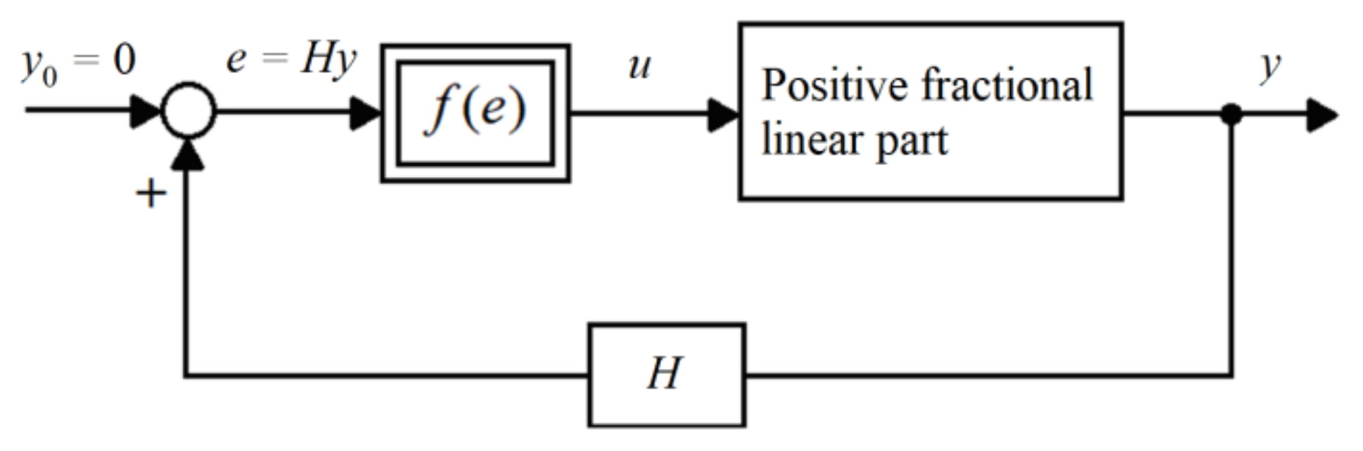
Consider the m-input p-output (MIMO) nonlinear feedback system shown in Figure 1 which consists of the positive fractional linear part, the nonlinear element with the matrix characteristic and the feedback with positive gain matrix H. The positive fractional linear part is described by the equations (25), (26) with the interval matrices
It is assumed that the interval matrix is Hurwitz.
The characteristic of the nonlinear element satisfies the condition
where
and
Remark 2.
The matrix K forms m, p-dimensional convex surfaces which constricts possible dynamics of nonlinear elements, i.e., for m = p = 1 the nonlinear characteristicf(e) is presented in Figure 2.
Definition 5.
The fractional nonlinear positive system is called globally stable if it is asymptotically stable for all nonnegative initial conditions
The following theorem gives sufficient conditions for the global stability of the positive nonlinear system.
Theorem 9.
The fractional nonlinear system consisting of the positive asymptotically stable linear part described by (25), (26) with interval matrices (33), the nonlinear element satisfying the condition (34) and the feedback with positive gain matrix is globally stable if the sum of entries of each column (row) of the matrix
is negative.
Proof.
The proof will be accomplished by the use of the Lyapunov method [26,27]. As the Lyapunov function we choose
where is a strictly positive vector, i.e., ,
Using (37) and (25) we obtain
since
From (39) it follows that if the sum of entries of each column (row) of the matrix (37) is negative (Theorem 3) and the nonlinear positive system is globally stable. □
5. Procedure and Example
To find the satisfying the condition (37) for the nonlinear positive system, the following procedure can be used.
Procedure 1.
- Step 1.
- Using the matrices of the positive linear system and the matrix compute the maximum value of the matrix such that the sum of all entries of each column (row) of the matrixis negative. Entries of the matrix can be computed as the solution of the linear matrix equationwhere the matrix and the column vector are defined by the sum of entries of each column (row) of the matrix (40) and vector k contains components of matrix K. If or/and then we choose arbitrarily nonnegative entries of the matrix K.
- Step 2.
- Using the matrices of the positive linear system and the matrix compute the maximum value of the matrix such that the sum of all entries of each column (row) of the matrixis negative.
- Step 3.
- Taking into consideration computed in Step 1 and from Step 2, find the desired for which the matrices and are Hurwitz, i.e., the characteristic f(e) satisfy the condition (34).
Remark 3.
The conditions of Theorem 2 can be also used to compute the entries of the matrix. Usually in this case the computations are more complicated.
Example 2.
Consider the nonlinear feedback system shown in Figure 1 with the interval matrices of the positive linear part
and the gain matrix
From (43) it follows that m = p = 2 and , then we are looking for
for which the nonlinear feedback system is globally stable.
Using Procedure 1 we obtain:
- Step 1.
- Using (40), (43) and (44) we determined that the sum of columns are the following:and taking into consideration (5.2), we haveSince , then we choose elements of the vector k (entries of the matrix K) as . The solution for (41) with (47) is the followingand forthe system with is stable.
- Step 2.
- Similar to Step 1, using (42), (43) and (44) we can write the linear matrix Equation (41) in the formSince , then we choose two elements of the vector k as . The solution for (50) isandTherefore, the system with is stable.
- Step 3.
- Taking into consideration (49) and (52), we have that forthe matrices and are Hurwitz sinceTherefore, for nonlinear elements satisfying the conditionthe nonlinear feedback system with interval matrices (43) of positive linear parts and for the gain matrix (53), the nonlinear system is globally stable.
6. Exponential Decay of Processes in Nonlinear Feedbacks Systems
Consider the nonlinear feedback system shown in Figure 3 which consists of the positive linear part, the nonlinear element with characteristic and positive dynamical feedback. The linear part is described by the equations
with interval matrices
where is the state, input and output vectors of the system (56) and It is assumed that the matrix of (56) has all eigenvalues with real parts smaller than
The characteristic of the nonlinear element is shown in Figure 2 and it satisfies the condition
The positive feedback system is described by the equations
with interval matrices
where are the state vector and output vectors. It is assumed that the matrix is also asymptotically stable. From (56) and (60) we have
where
The following theorem gives sufficient conditions for the exponential decay of transient values in the positive feedback nonlinear system faster than .
Theorem 10.
The state variables of the nonlinear system consisting of the positive linear part (56), the nonlinear element satisfying the condition (34), (35), (36) and positive asymptotically stable dynamical feedback system (60) are decaying exponentially faster than if the matrix
is asymptotically stable.
Proof.
It is well-known that if the matrix is asymptotically stable, then the state variables of the system are decaying exponentially faster than .
Using (56), (60) and (65) we obtain
since by the condition (6.2).
From (66) it follows that if the matrix (64) is asymptotically stable, and therefore the state variables decay exponentially faster than . □
Theorem 6.1 can be applied to solve the following two problems.
Problem 1.
Given matrices A, B, C and F, G, H of the positive systems (56), (60) and the nonlinear characteristic of the nonlinear element. Knowing the value of satisfying the condition (59), check if the transient processes in the nonlinear system decay faster than .
Problem 2.
Given matrices A, B, C and F, G, H of the positive systems (56), (60) and the nonlinear characteristic of the nonlinear element. Find the maximal value of for which the characteristic of the nonlinear element satisfies the condition (59) and the transient values of the nonlinear system decay faster than .
The Problem 1 can be solved by the use of the following:
Procedure 2.
- Step 1.
- Knowing the characteristic , find the minimal value of satisfying the condition (59).
- Step 2.
- Using Theorem 10, find the sum of entries of each column (row) of the matrix (64). If all these sums are negative, then the transient processes in the nonlinear system decay faster than .
The Problem 2 can be solved by the use of the following:
Procedure 2.
- Step 1.
- Using Theorem 10, find the sum of entries of each column (row) of the matrix (64).
- Step 2.
- Find the maximal value of for which the sums of entries of all columns (rows) of (64) are negative.
- Step 3.
- Find .
In this case, the transient process in the nonlinear system decrease faster than for all nonlinear characteristics satisfying the condition
Remark 4.
The value ofdepends only on the firstrows and of the lastcolumns of the matrix (64).
Example 3.
Consider the nonlinear system shown in Figure 3 with linear positive parts described by (56) and (60) with
and
respectively, and the nonlinear element with characteristics satisfying the condition (59).
Case 1.
Using, check the global stability of the nonlinear system forIn this case, using (6.5), (6.9) and (6.10) we obtain
The sums of the entries of columns of the matrix (6.11) are: column 1:column 2:column 3:column 4:. Therefore, by Theorem 6.1, the nonlinear system is globally stable.
Case 2.
Find the maximal value ofsatisfying the condition (4.2) for which the transient process in the nonlinear system decreases faster than. Using Procedure 2 we obtain the following:
- Step 1.
- The sums of entries of each column (row) of the matrixare: column 1:column 2:column 3:column 4:row 1:row 2:row 3:row 4:
- Step 2.
- From Theorem 10 we have: for column 3: k < 3.428 and for column 4: k < 5.357 and for row 1: k < 6.482, row 2: k < 3.0555.
- Step 3.
- The desired value of k is.Therefore, the transient process in the nonlinear system with characteristics satisfying the condition (34), (35), (36) fordecreases faster than.
Remark 3.
From matrix (6.5) and the computation procedure, it follows that the k depends only on the matrices F, G, H and is independent of the matrices A, C, G.
7. Concluding Remarks
The global stability of continuous-time nonlinear feedback systems with different fractional orders and interval matrices of positive linear parts has been investigated. New sufficient conditions for the global stability of this class of positive nonlinear systems are established (Theorem 9). The procedure for the calculation of a gain matrix characterizing the class of nonlinear elements is presented and illustrated by numerical example. Sufficient conditions for the exponential decay of processes in nonlinear systems have been proposed (Theorem 10) and illustrated by numerical example. The considerations can be extended to the discrete-time nonlinear systems with different fractional orders and interval matrices of positive linear parts. Further investigation could address the extension of the considerations to nonlinear different fractional order systems with e time-varying linear parts.
Author Contributions
Conceptualization, T.K. and Ł.S.; methodology, T.K.; formal analysis, T.K.; writing—original draft preparation, Ł.S.; writing—review and editing, Ł.S.; supervision, T.K.; funding acquisition, T.K. and Ł.S. All authors have read and agreed to the published version of the manuscript.
Funding
This work was supported by National Science Centre in Poland under work No. 2017/27/B/ST7/02443.
Institutional Review Board Statement
Not applicable.
Informed Consent Statement
The study did not involve humans.
Data Availability Statement
The study did not report any data.
Conflicts of Interest
The authors declare no conflict of interest.
References
- Berman, A.; Plemmons, R.J. Nonnegative Matrices in the Mathematical Sciences; SIAM: Philadelphia, PA, USA, 1994. [Google Scholar]
- Farina, L.; Rinaldi, S. Positive Linear Systems: Theory and Applications; J. Wiley: New York, NY, USA, 2000. [Google Scholar]
- Kaczorek, T. Positive 1D and 2D Systems; Springer: London, UK, 2002. [Google Scholar]
- Kaczorek, T. Selected Problems of Fractional Systems Theory; Springer: Berlin, Germany, 2011. [Google Scholar]
- Kaczorek, T.; Rogowski, K. Fractional Linear Systems and Electrical Circuits; Springer: Cham, Switzerland, 2015. [Google Scholar]
- Ostalczyk, P. Discrete Fractional Calculus; World Scientific: River Edgle, NJ, USA, 2016. [Google Scholar]
- Podlubny, I. Fractional Differential Equations; Academic Press: San Diego, CA, USA, 1999. [Google Scholar]
- Busłowicz, M.; Kaczorek, T. Simple conditions for practical stability of positive fractional discrete-time linear systems. Int. J. Appl. Math. Comput. Sci. 2009, 19, 263–269. [Google Scholar] [CrossRef] [Green Version]
- Kaczorek, T. Absolute stability of a class of fractional positive nonlinear systems. Int. J. Appl. Math. Comput. Sci. 2019, 29, 93–98. [Google Scholar] [CrossRef] [Green Version]
- Kaczorek, T. Analysis of positivity and stability of fractional discrete-time nonlinear systems. Bull. Pol. Acad. Sci. Techn. 2016, 64, 491–494. [Google Scholar] [CrossRef] [Green Version]
- Kaczorek, T. Positive linear systems with different fractional orders. Bull. Pol. Acad. Sci. Techn. 2010, 58, 453–458. [Google Scholar] [CrossRef]
- Kaczorek, T. Positive linear systems consisting of n subsystems with different fractional orders. IEEE Trans. Circuits Syst. 2011, 58, 1203–1210. [Google Scholar] [CrossRef]
- Kaczorek, T. Positive fractional continuous-time linear systems with singular pencils. Bull. Pol. Acad. Sci. Techn. 2012, 60, 9–12. [Google Scholar] [CrossRef] [Green Version]
- Kaczorek, T. Stability of fractional positive nonlinear systems. Arch. Control. Sci. 2015, 25, 491–496. [Google Scholar] [CrossRef]
- Mitkowski, W. Dynamical properties of Metzler systems. Bull. Pol. Acad. Sci. Techn. 2008, 56, 309–312. [Google Scholar]
- Ruszewski, A. Stability of discrete-time fractional linear systems with delays. Arch. Control Sci. 2019, 29, 549–567. [Google Scholar]
- Ruszewski, A. Practical and asymptotic stabilities for a class of delayed fractional discrete-time linear systems. Bull. Pol. Acad. Sci. Techn. 2019, 67, 509–515. [Google Scholar]
- Sajewski, Ł. Decentralized stabilization of descriptor fractional positive continuous-time linear systems with delays. In Proceedings of the 22nd International Conference Methods and Models in Automation and Robotics, Międzyzdroje, Poland, 28–31 August 2017; pp. 482–487. [Google Scholar]
- Sajewski, Ł. Stabilization of positive descriptor fractional discrete-time linear systems with two different fractional orders by decentralized controller. Bull. Pol. Acad. Sci. Techn. 2017, 65, 709–714. [Google Scholar] [CrossRef] [Green Version]
- Borawski, K. Modification of the stability and positivity of standard and descriptor linear electrical circuits by state feedbacks. Electr. Rev. 2017, 93, 176–180. [Google Scholar] [CrossRef] [Green Version]
- Kaczorek, T.; Borawski, K. Stability of Positive Nonlinear Systems. In Proceedings of the 22nd International Conference Methods and Models in Automation and Robotics, Międzyzdroje, Poland, 28–31 August 2017. [Google Scholar]
- Kaczorek, T. Superstabilization of positive linear electrical circuit by state-feedbacks. Bull. Pol. Acad. Sci. Techn. 2017, 65, 703–708. [Google Scholar] [CrossRef] [Green Version]
- Kaczorek, T. Global stability of positive standard and fractional nonlinear feedback systems. Bull. Pol. Acad. Sci. Techn. 2020, in press. [Google Scholar]
- Kaczorek, T. Analysis of positivity and stability of discrete-time and continuous-time nonlinear systems. Comput. Probl. Electr. Eng. 2015, 5, 11–16. [Google Scholar]
- Kaczorek, T. Global stability of nonlinear feedback systems with positive linear parts. Int. J. Nonlinear Sci. Numer. Simul. 2019, 20, 575–579. [Google Scholar] [CrossRef]
- Lyapunov, A.M. Obscaja Zadaca ob Ustoicivosti Dvizenija; Gostechizdat: Moskwa, Russia, 1963. [Google Scholar]
- Leipholz, H. Stability Theory; Academic Press: New York, NY, USA, 1970. [Google Scholar]
Figure 1.
The nonlinear feedback system.

Figure 2.
Characteristic of single-input single-output nonlinear element.

Figure 3.
The nonlinear feedback system.

Publisher’s Note: MDPI stays neutral with regard to jurisdictional claims in published maps and institutional affiliations. |
© 2021 by the authors. Licensee MDPI, Basel, Switzerland. This article is an open access article distributed under the terms and conditions of the Creative Commons Attribution (CC BY) license (https://creativecommons.org/licenses/by/4.0/).
Share and Cite
MDPI and ACS Style
Kaczorek, T.; Sajewski, Ł. Global Stability and Exponential Decay of Processes in Nonlinear Feedback Systems with Different Fractional Orders. J 2021, 4, 328-340. https://0-doi-org.brum.beds.ac.uk/10.3390/j4030025
AMA Style
Kaczorek T, Sajewski Ł. Global Stability and Exponential Decay of Processes in Nonlinear Feedback Systems with Different Fractional Orders. J. 2021; 4(3):328-340. https://0-doi-org.brum.beds.ac.uk/10.3390/j4030025
Chicago/Turabian StyleKaczorek, Tadeusz, and Łukasz Sajewski. 2021. "Global Stability and Exponential Decay of Processes in Nonlinear Feedback Systems with Different Fractional Orders" J 4, no. 3: 328-340. https://0-doi-org.brum.beds.ac.uk/10.3390/j4030025