Semi-Dilute Dumbbells: Solutions of the Fokker–Planck Equation


School of Mathematics and Statistics, University of Sheffield, Hicks Building, Hounsfield Road, Sheffield S3 7RH, UK
*
Author to whom correspondence should be addressed.
†
Current address: School of Mathematics, University of Leeds, Leeds LS2 9JT, UK.
‡
These authors contributed equally to this work.
J 2021, 4(3), 341-355; https://0-doi-org.brum.beds.ac.uk/10.3390/j4030026
Submission received: 21 June 2021
/
Revised: 7 July 2021
/
Accepted: 12 July 2021
/
Published: 14 July 2021
(This article belongs to the Section Computer Science & Mathematics)
Abstract
:Spring bead models are commonly used in the constitutive equations for polymer melts. One such model based on kinetic theory—the finitely extensible nonlinear elastic dumbbell model incorporating a Peterlin closure approximation (FENE-P)—has previously been applied to study concentration-dependent anisotropy with the inclusion of a mean-field term to account for intermolecular forces in dilute polymer solutions for background profiles of weak shear and elongation. These investigations involved the solution of the Fokker–Planck equation incorporating a constitutive equation for the second moment. In this paper, we extend this analysis to include the effects of large background shear and elongation beyond the Hookean regime. Further, the constitutive equation is solved for the probability density function which permits the computation of any macroscopic variable, allowing direct comparison of the model predictions with molecular dynamics simulations. It was found that if the concentration effects at equilibrium are taken into account, the FENE-P model gives qualitatively the correct predictions, although the over-shoot in extension in comparison to the infinitely dilute case is significantly underpredicted.

1. Introduction
Spring bead models prove to be an effective way to construct constitutive equations for polymer melts. Perhaps the most widely used with success is the finitely extensible nonlinear elastic (FENE) dumbbell model, which exhibits a viscous response that arises from Brownian motion and an elastic response that arises from the spring connecting the beads [1]. However, single dumbbell models are just a simple approximation to polymer melt solutions and do not reflect all the complex physical processes that can occur. Augmented dumbbell models have been developed that include additional effects such as internal viscosities [2,3], additional hydrodynamic interactions [4,5,6], and aniostropic drag [7]. These advances resulted in a computationally viable constitutive model, allowing improved predictions and greater understanding of single polymer experiments [8,9,10,11].
The aim of this article is to further investigate the mean-field model proposed by Schneggenburger et al. [12], which also incorporated concentration effects and weak shear. This model is revisited in [13] to include steady uniaxial elongation within the Hookean regime. The behavior of the FENE dumbbell model without the mean-field term is well understood and has been extensively studied [14,15]. The mean-field model under uniform weak shear-flow conditions gives good predictions of the orientation angle and qualitative predictions of the radius of gyration when compared with light scattering experiments [12,16]. Concentration effects have been quantified experimentally under equilibrium conditions and for shear flows [16,17,18]. Concentration-induced effects were found to be more significant in elongational flows than in shear flows [19]. A study using a four-roll mill found that increases in concentration effects result in a reduction of the extension due to polymer entanglement [20]. A later study using a FENE-CR fluid to model the full four-roll mill system found qualitative agreement with experiments [21]. This reduction in extension due to semi-dilute behaviors has also been reported experimentally [22], in Brownian dynamical simulations [23] and from modified dumbbell models [24].
In this paper, we will extend the investigations in [12,13], the authors of which solved the constitutive equations for the second moment. We will include the effects of strong shear and large elongation. Further, we will explore the form of the probability density function, , which permits the computation of any macroscopic variable, thus enabling direct comparisons of the FENE dumbbell model with molecular dynamics simulations. The paper is structured as follows. The governing equations are introduced in Section 2. The equations are solved Section 3, with results presented for the dumbbell model with mean-field force under strong shear and elongation. Finite element solutions of the FENE model incorporating the Peterlin closure approximation (FENE-P) are also presented, along with results of molecular dynamics simulations. Results are discussed and conclusions drawn in Section 4.
2. Materials and Methods
The Governing Equations
We will model the fluid as a suspension of dumbbells embedded in a Newtonian solvent. The dumbbells comprise two beads connected by a spring. The behavior of the dumbbell can be completely described by the vector that connects the location of one of the beads to the other. The governing equations are expressed solely in terms of . To form the equations that describe the evolution of , an elastic law for the spring must be proposed. We adopt the FENE relation for the spring force ,
where H is a spring constant and is the maximum possible extension of the dumbbells [1]. Taking the limit , the linear Hookean spring law is recovered, which microscopically reduces to the Oldroyd B model. In the limit at which the end-to-end vector reaches its maximum extension, the fluid acts analogous to a suspension of infinitely thin rigid rods. (1) is an empirical approximation to the physically derived inverse Langevin operator [25]. Other approximations could have been used, for instance, the Marko–Siggia force law [26], the Padé law [27], or improved closure approximation modifications such as the FENE-L model [28,29].
The equation of motion for an individual dumbbell can be found from the spring law. Assuming that the velocity field is homogeneous over the length scale of the polymer, then the evolution of is given by the Langevin equation [30]:
Here, denotes the mean-field forces, k is the Boltzmann constant, T is the absolute temperature, and is the drag constant. The tensor is the transpose of the velocity gradient given by . The Brownian term is a Wiener process whose components are independent Gaussian variables with mean zero and variance . The Langevin equation has an equivalent Fokker–Planck (FP) equation for the probability distribution . The evolution equation for is given by the partial differential equation
The velocity field is given by
where is the elongation rate. We adopt the mean-field force term used in [12,31],
The mean-field term is introduced to model weak anisotropic effects from concentration effects due to intra- and intermolecular interactions. The parameter f determines the strength of the mean-field term and is a positive function of the concentration. For infinitely dilute solutions, . f increases with increasing concentration by , where is a reference concentration. denotes the the deviatoric part of the symmetric decomposition of a tensor . Equation (5) was derived from studies of rod-like polymers [32]. At equilibrium, when is isotropic, there is no preferential direction and the mean-field term becomes zero.
For finite , the system cannot be solved analytically as a closed constitutive equation cannot be formed from only the second moment, or radius of gyration tensor, . A closed system can be formed if the Hookean spring force is used; however, in elongational flows, one can expect the solution to be valid over a small range of elongation rates only due to the dumbbells becoming infinitely extended. The standard approach to overcome this closure problem is to replace the spring force model in (1) with the pre-averaged Peterlin closure approximation in which the nonlinear Wagner spring force term is approximated by a self-consistent average term [33]. This results in a spring force model of the form
This has the advantage that the nonlinear finite extensiblity term is now linear with respect to the microscopic variables.
3. Results
3.1. Mean-Field Force under Elongation
We now seek an exact solution to (3) for homogeneous planar elongational flow with elongation rate . This was first investigated in [13]. We extend their analysis to investigate the non-Hookean response. We will use the convention that is the velocity gradient tensor, i.e., . For purely planar elongational flow, is given by , where is the Kronecker delta function. To find a steady-state solution, we adopt a change of variable approach by writing , where and: denotes full index contraction. This form of solution is motivated by solutions of the FP equation found for elongational flows in [30]. This removes the advective term and the FP equation reduces to
As we are concerned with pure elongational flow, we can assume a priori that the shear term . Thus, the tensor product term in (5) can be written as
where implies no summation over the elements. It follows that at the microscopic level the spring force is now a scalar multiplied by the end-to-end vector. This additional force acts analogous to a Hookean spring with non-constant H, where the spring constant is a function of the macroscopic variables. Thus we can write a solution for the probability distribution as
To simplify the notation, we replace , , , by , y and introduce the characteristic spring time, . The variables and are given by
Physically is a measure of the anisotropy that arises solely from mean-field effects and acts like an additional elongation rate. and are not free variables as they have a hidden dependency on . They can be determined by the averaging conditions
Adopting the scalings , , and , we obtain
The parameter, , is the ratio of the flexible spring time to the characteristic rigid time . Physically b represents the number of monomers in the polymer [34]. Dropping the for convenience, we recover a system of nonlinear algebraic equations:
3.2. Mean-Field Force under Shear
The effects of concentration dependent shear-induced anisotropy were investigated in [12] by means of solving the constitutive equation for the second moment. However, at no extra computational cost, we can obtain which permits the computation of any macroscopic variable, thus enabling direct comparison of the predictions of the model with molecular dynamics simulations.
In contrast to the case for elongational flow, it is clear that the term will be non-zero and thus a different approach must be taken. For Hookean dumbbells under shear flow with no mean-field dependence, the velocity gradient tensor is given by , where is the Kronecker delta function, and the FP equation has solution [30] takes the form
For the analogous case, which includes a mean-field force under shear, we anticipate that the solution is of a similar form as (18), and seek a trial solution of the form
where are constants to be determined. We need not restrict ourselves to pure shear flow but could consider a flow field that exhibits both elongational and shear phenomena. We take a general homogeneous velocity gradient field for which the velocity components are given by and . Substitution of this trial solution into the FP equation leads to
where and . The symbol ∘ denotes array-wise multiplication. We find
The mean-field term is decomposed into a shear-like component and an elongation-like component: , by means of two basis vectors, and . Therefore,
which is analogous to the solution for with modified shear rate and modified elongation rate . From (21) the parameters are
where and . In the limit as f tends to zero (i.e., ) and the standard Hookean solution (18) is recovered. The normalization constant J can be expressed as . The consistency conditions for the system naturally give rise to an equivalent set of equations as derived by [12] who used a change of basis method. The two conditions (11) and (12) still hold, however, as no ansatz is used regarding , the extra degree of freedom is accounted for by an additional consistency condition. We can write
Use of the aforementioned scalings, with the shear rate scaling analogous to the elongation rate (i.e., ), leads to the system of equations (with the star notation dropped),
which are again solved by the Newton–Raphson method. It can be seen that for elongational flow, increasing f leads to greater stretching of the dumbbell. For shear flows, increasing f leads to greater orientation of the dumbbell along the flow. We will now compare these results to those of the full nonlinear FENE model. The expansion for small was previously obtained in [12], however the effect for large shear was not addressed. We will consider this effect by using the method of dominant balance [35]. This results in the expressions
These series exhibit much better convergence than those for elongational flow. We see that the effects of concentration increase the radius of gyration. These effects decay as , which is a slower decay than for the elongational case, where the decay is proportional to . An interesting feature of shear flows is that the degree of shear changes the orientation of the dumbbells. The orientation angle is given by [36]
As , the angle of orientation is as expected and the dominant effect is the finite extension force. We see that the mean-field term which decays as has opposite sign to the finite extension effect and acts so as to resist the orientation of the dumbbell.
3.3. FENE Solution
An iterative finite element scheme was used to solve the FP equation with the inclusion of the fully nonlinear FENE force term. Although the Peterlin closure approximation removes the unwanted infinite elongation that occurs with Hookean spring models, it only imposes a constraint on the averaged value of the end-to-end vector rather than an upper-bound, thus dumbbells can exist which have length greater than [37]. Furthermore, the effect of the Peterlin closure approximation is non-local. The distribution for the FENE-P model is Gaussian whereas the FENE model cannot have a chain length greater than the maximum extension that gives compact support. This difference in the FENE-P model has previously been shown to effect the transient response as well [14]. In this study, we limit our investigation to steady state flows. We will use the notation that is the computational domain and is the bounding region. Under purely elongational flow, the FP equation is solved for radius , which arises from the FENE model restricting the radius of gyration. To reduce the computational domain, we consider the upper quadrant and impose symmetry boundary conditions along the and axes. The Dirichlet condition, , is applied on the boundary , which enforces zero probability of the dumbbell being fully extended. Strong symmetry does not exist for the pure shear case and the FP equation must be solved over the entire circular domain. As such a system has purely homogeneous boundary conditions, the trivial zero solution would be recovered. To overcome this we add a point constraint on the probability at the origin where the constant is determined by requiring conservation of probability.
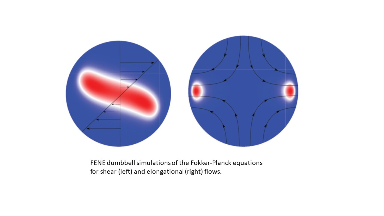
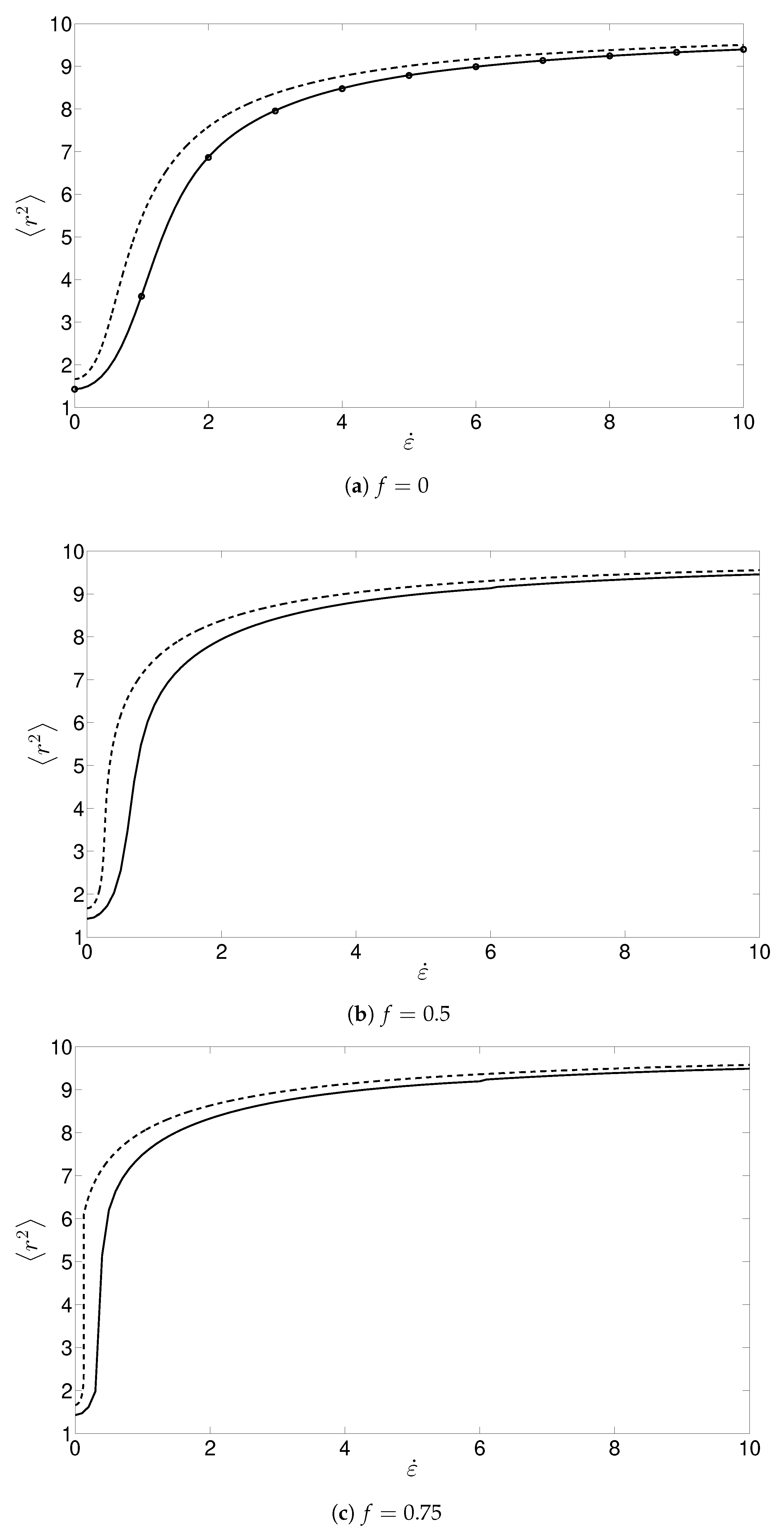
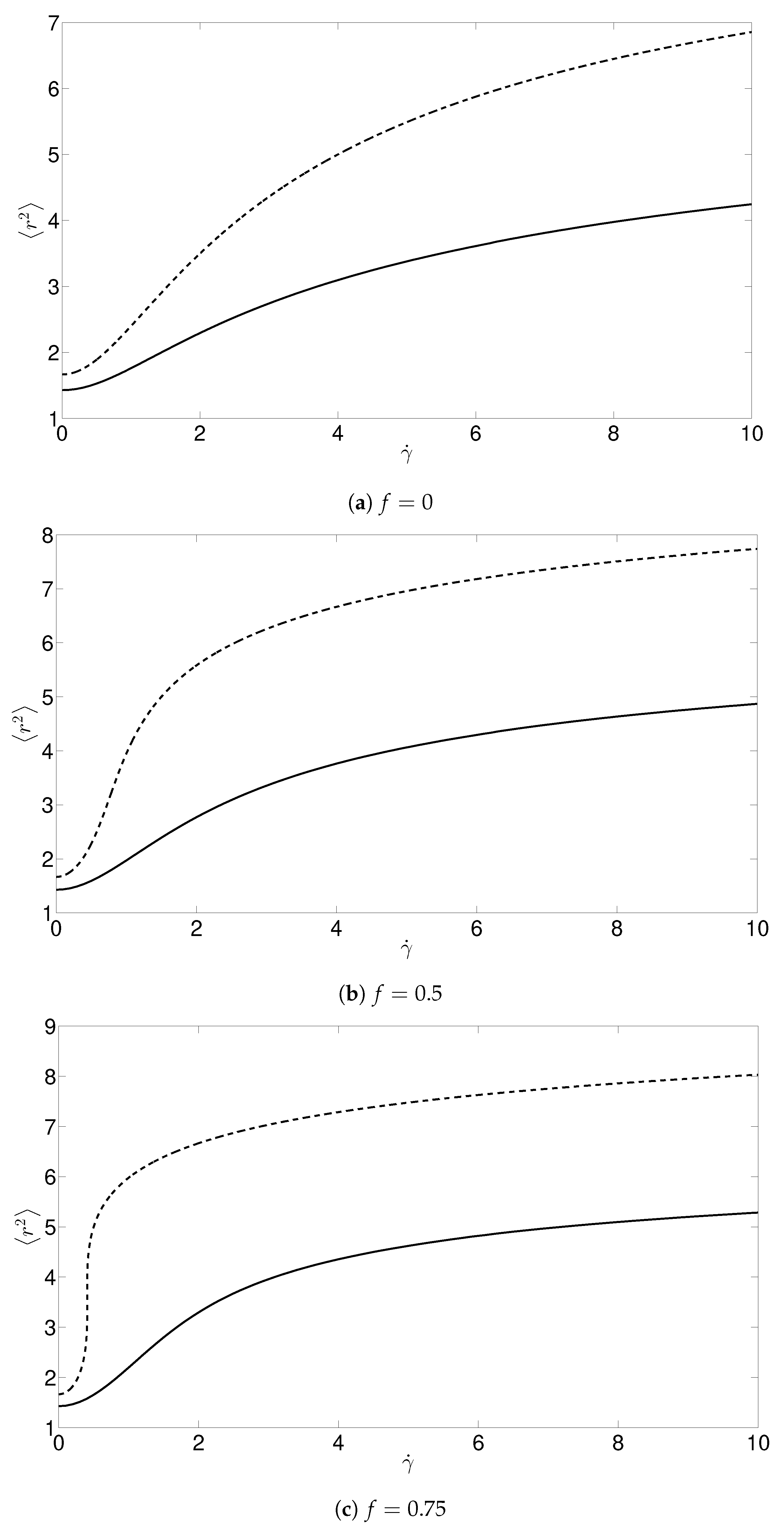
Simulations from FENE and FENE-P schemes for elongational flow are shown in Figure 1 and Figure 2 for , 0.5 and 0.75. The analytical solution for is given by where N is the appropriate normalization constant [7]. This is in close agreement with the results from the finite element solution (Figure 2a). Plots of the radius of gyration calculated from the FENE and FENE-P models for , 0.5, and 0.75 for the case of shear flow are shown in Figure 3. It was found that for large elongation rates, use of the Peterlin closure approximation (Figure 2) gave similar results to the FENE model for the dependence of the radius of gyration on the non-dimensionalized elongation rate. However, the Peterlin closure approximation systematically overestimated the radius of gyration. For the case , the overestimation can be explained as the finite extension is imposed only on the average extension. We also found that the greatest error occurs for moderately small elongation rates. The magnitude of the error is increased and the maximum peak error occurs at a lower elongation rate for increasing values of f. This error is due to the relatively large gradients of the radius of gyration with respect to the elongation rate. These large gradients are due to coil stretch transition and are eventually smoothed when the finite extensibility constraint starts to dominate.For shear flow with , the error increases monotonically with shear rate. However, with the introduction of the mean-field term the peak error occurs at a finite shear rate. The effect of increasing f is similar, but less pronounced than the effect seen with elongational flows, where the magnitude of the error increases and occurs at a lower shear rate.
Using the previous scaling, while dropping the , the steady-state FP equation with the inclusion of a mean-field term for elongational flow is given by
where and are the unit vectors in the x- and y-directions.
Equation (31) does not account for the following two constraints. Firstly, that , and second, upon scaling of , the condition of which introduces nonlinearity in . To approach these conditions a fixed point finite element iterative scheme is used to reach a default tolerance:
where denotes the weak form of (31). Equation (31) can be similarly formed and solved for the case of pure shear flow which in weak form is
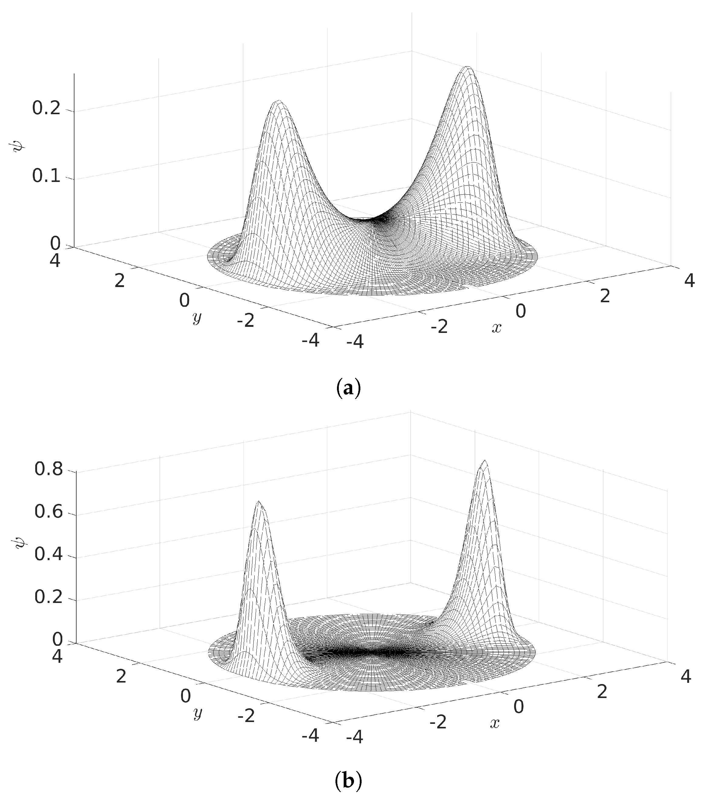
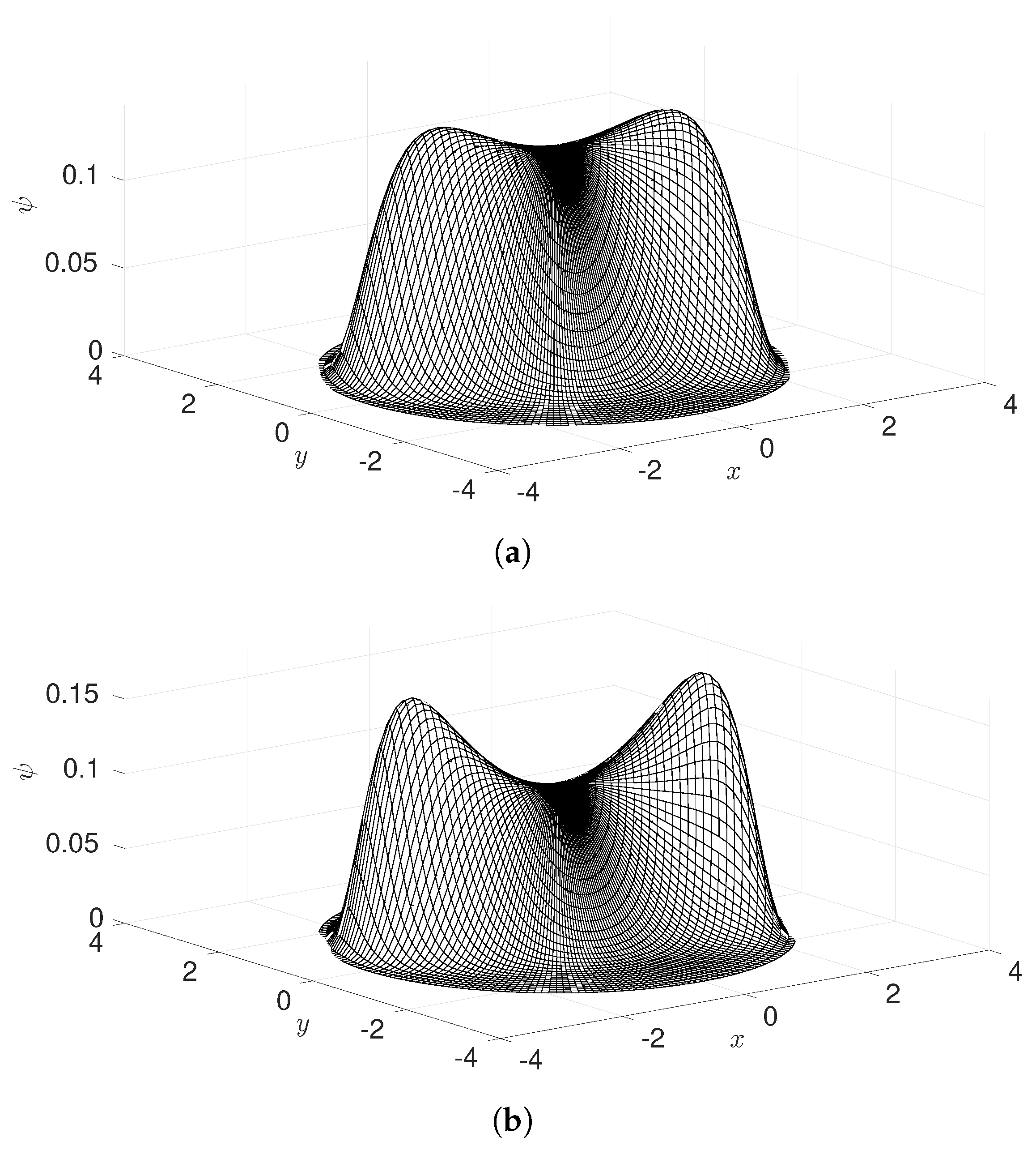
where gives the shape function. The velocity gradient tensor, , takes a different form for shear and elongational flows. The Galerkin finite element method was used, where comprised linear piecewise polynomials. The stiffness matrix was formed from the first term which is integrated using a fourth order quadrature method over a triangular mesh with 40,000 nodes. The mesh density was increased near , as well as along for the elongational case, to capture the larger gradients in . The advective term is the only term which changes and is initially set to be 0. is found through the iterative scheme (32)–(34). The probability density function is plotted for the FENE solution for the case of pure elongational flow in Figure 4. The effects of the additional concentration are similar to those obtained using the Peterlin closure approximation where the concentration term acts analogously to the elongation term and gives rise to increased probability of larger extensions of the dumbbells. The effect is similar, but smaller, for the case of pure shear flow as shown in Figure 5.
3.4. Comparison with Molecular Dynamics Simulations
The predictions of the FENE-P model were compared with stochastic data [23]. The FENE-P model predicts that with increasing f, the mean-field effect will increase the mean extension of the dumbbell. It can be seen from (7) and (8) that the spring stiffness constant reduces for increasing f. This feature is opposite to that which is reported in the literature. One possible explanation is that in the model used in [12] the equilibrium radius of gyration is independent of concentration. However, the authors of [23] report that the equilibrium radius of gyration can vary with concentration. We model the equilibrium mean-field effects by expressing the parameter b as a function of the concentration. We model b as a quadratic in , i.e.,
where the parameters are found by fitting to the profile of the equilibrium results for given in [23]. Stoltz et al. [23] determined the extension as a function of both the relaxation time and the concentration dependent relaxation time (CDRT). The CDRT is found by modeling the experimental procedure in [18], in which the polymer was stretched under elongational flow and then allowed to relax back to equilibrium. The CDRT was found by fitting an exponential function to the transient profile of the radius of gyration. Stoltz et al. [23] record the affect of concentration on the mean distance between the end points only in streamwise direction and not the radius of gyration. This can be found using probability density function (9) to be
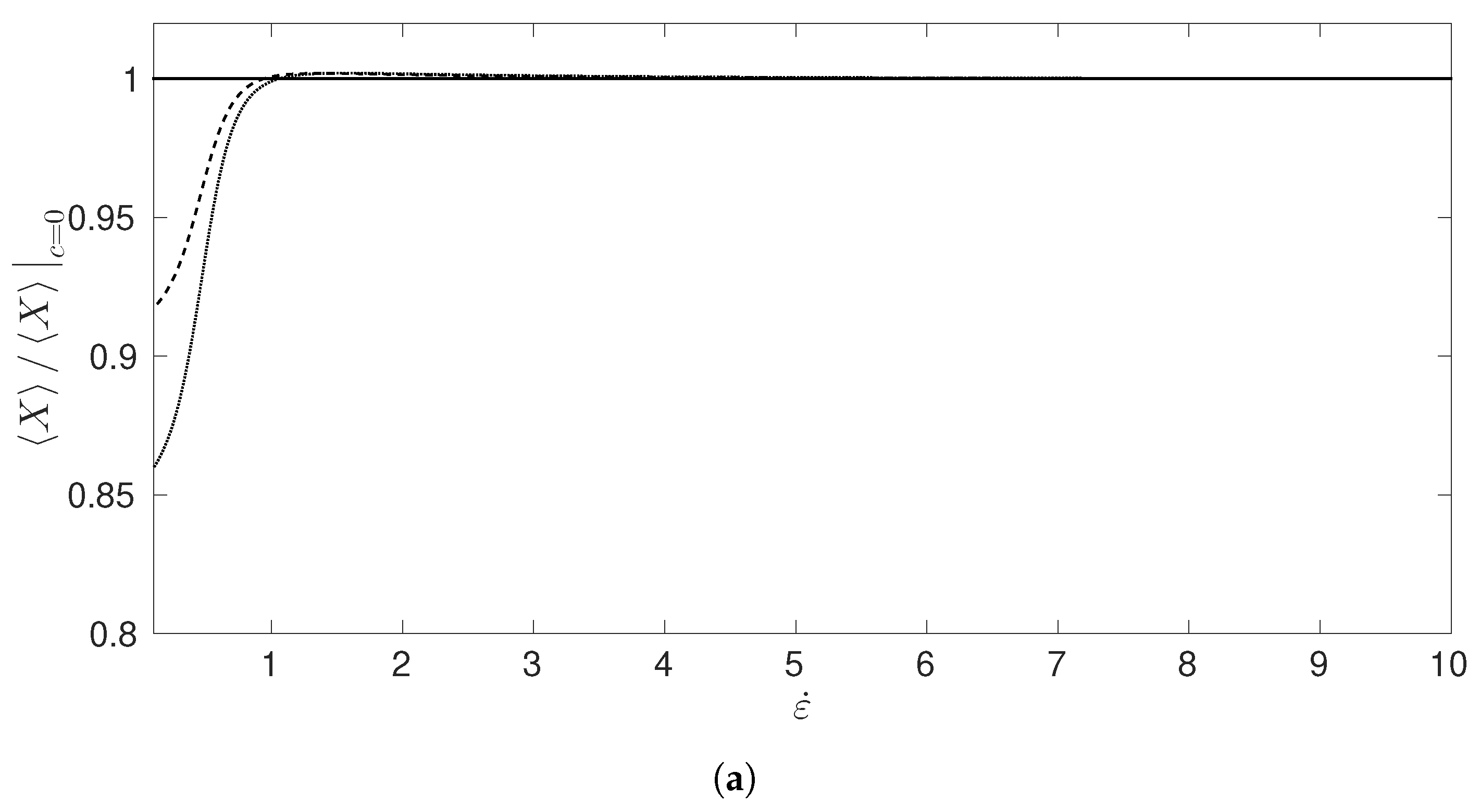
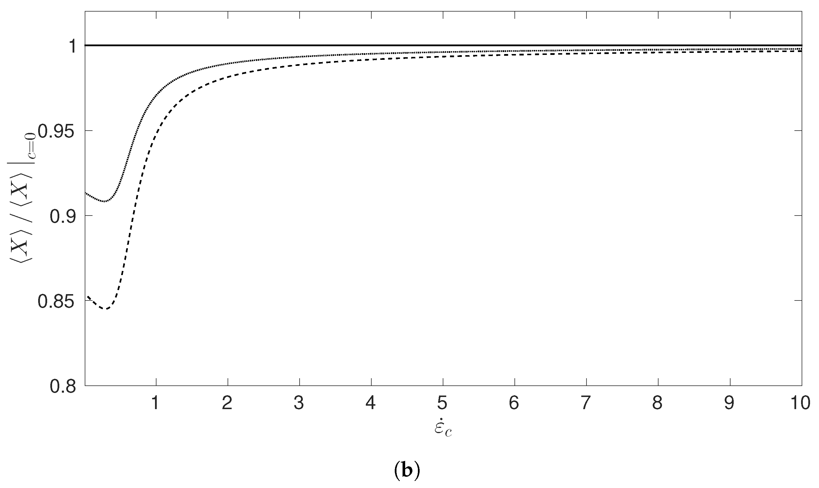
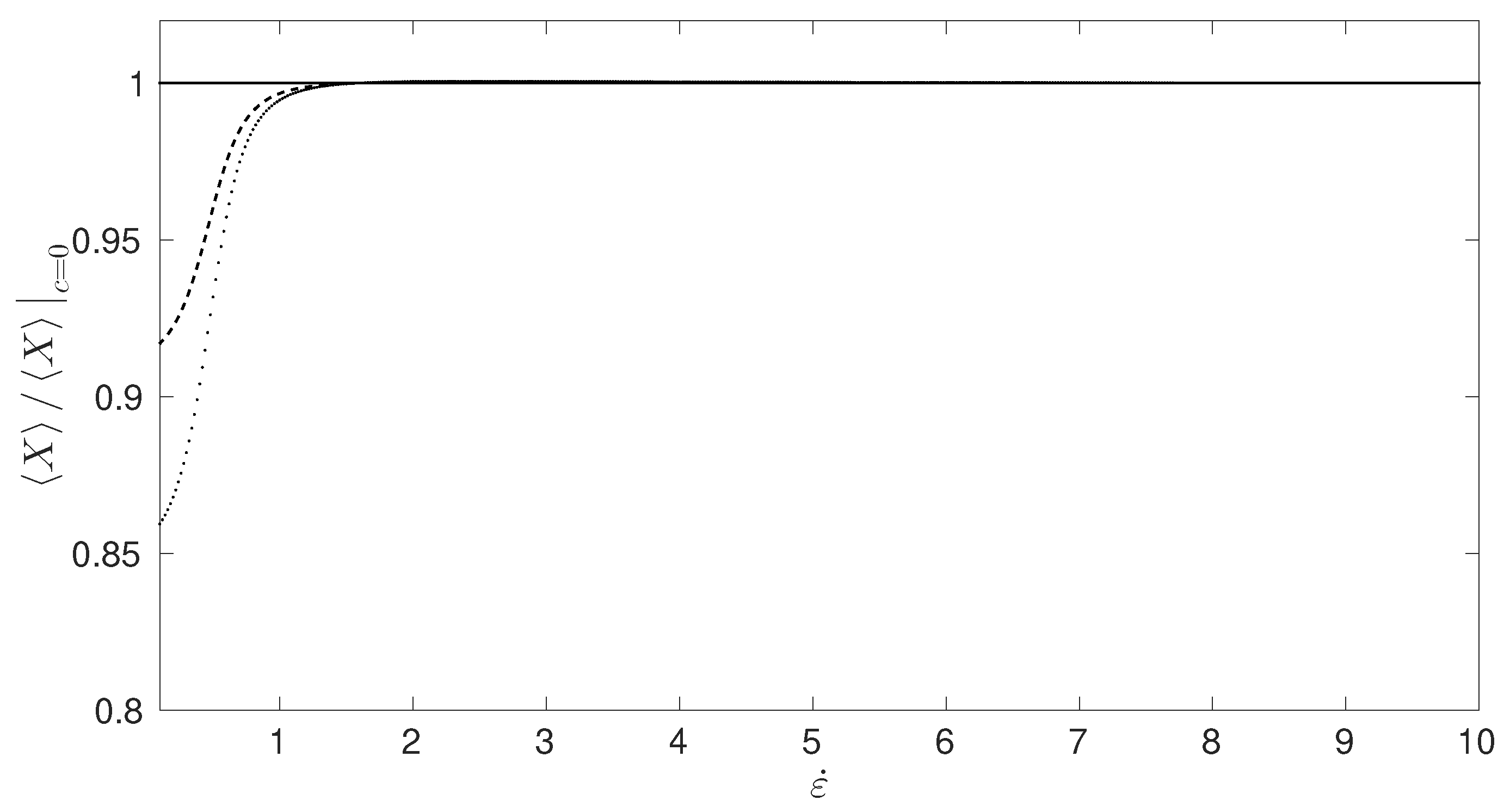
We chose for our simulations as the results were found to be largely independent of provided it was sufficiently large. Figure 6 shows plots of normalized by its value for large extension against the elongation rate and against the critical elongation rate . The model now predicts that the end-to-end distance is reduced for increasing concentration when plotted against . For comparison, is plotted in Figure 7, for the case where the mean-field force term was set to zero. If we look at the normalized values of corresponding to we observe a small overshoot in for the case where the mean-field term is included (Figure 6a). Such an overshoot does not occur in the simulations where this term has been neglected (Figure 7). A similar phenomena was reported in [23], although in their study, the size of the overshoot was more pronounced.
4. Discussion
The principle result of this article was the derivation of solutions to the Fokker–Planck equation incorporating a FENE-P dumbbell model with the addition of a mean-field term for both shear and elongational flows, including the effects of strong shear and elongations close to the maximum permissible. We found that the results corresponding to elongational flow were amenable to analytical analysis. For a linear spring force, the distribution can be found exactly and for dumbbells near full extension, an exact solution was found that could be expressed as the root of a quartic equation. The solution for a constant shear flow was found by directly solving the Fokker–Planck equation. We further investigated the effect that the closure assumption on the spring force has on the model. The probability density function was found numerically using a finite element scheme. We found that the closure assumption in conjunction with the mean-field term led to an over-estimation of the extension of the dumbbell at moderate values of the elongation and shear rate. In the latter part of the work, we matched the prediction of the model to molecular dynamics simulations. It was found that the model developed by [12] fails to predict the reduced stretching that occurs with increasing concentration. We thus proposed a novel extension by introducing a concentration dependence on the parameter b, which describes the ratio of the flexible spring time to the characteristic rigid time, to match the results given in [23], which were based on stochastic data. This modified model correctly predicted reduced stretching with increased concentration; however, the overshoot in relation to the infinitely dilute case in the aligned end-to-end vector was underpredicted.
Throughout this article we have only considered mean-field effects under steady shear and steady elongation conditions. This leaves the areas of transient shear and elongation open to further study.
Author Contributions
Conceptualization, S.C. and J.R.; methodology, S.C.; software, S.C.; validation, S.C.; formal analysis, S.C. and J.R.; investigation, S.C.; resources, J.R.; data curation, S.C.; writing—original draft preparation, S.C.; writing—review and editing, J.R.; visualization, S.C.; supervision, J.R.; project administration, J.R.; funding acquisition, J.R. All authors have read and agreed to the published version of the manuscript.
Funding
This research received no external funding.
Conflicts of Interest
The authors declare no conflict of interest.
Abbreviations
The following abbreviations are used in this manuscript:
| CDRT | Concentration dependent relaxation time |
| FENE | Finitely extensible nonlinear elastic |
| FENE-P | Finitely extensible nonlinear elastic with the Peterlin approximation |
| FP | Fokker–Planck |
References
- Warner, H.R. Kinetic theory and rheology of dilute suspensions of finitely extendible dumbbells. Ind. Eng. Chem. Fundam. 1972, 11, 379–387. [Google Scholar] [CrossRef]
- Adelman, S.A.; Freed, K.F. Microscopic theory of polymer internal viscosity: Mode coupling approximation for the rouse model. J. Chem. Phys. 1977, 64, 1380–1393. [Google Scholar] [CrossRef]
- Allegra, G. Internal viscosity in polymer chains: A critical analysis. J. Chem. Phys. 1986, 84, 5881–5890. [Google Scholar] [CrossRef]
- Farago, J.; Meyer, H.; Baschnagel, J.; Semenov, A.N. Hydrodynamic and viscoelastic effects in polymer diffusion. J. Condens. Matter Phys. 2012, 82, 284105–340000. [Google Scholar] [CrossRef]
- Ma, H.B.; Graham, M.D. Theory of shear-induced migration in dilute polymer solutions near solid boundaries. Phys. Fluids 2005, 17, 083103. [Google Scholar] [CrossRef] [Green Version]
- Ottinger, H.C. A model of dilute polymer solutions with hydrodynamic interaction and finite extensibility. I. Basic equations and series expansions. J. Non-Newton. Fluid Mech. 1987, 26, 207–246. [Google Scholar] [CrossRef]
- Bird, R.B.; Wiest, J.M. Anisotropic effects in dumbbell kinetic-theory. J. Rheol. 1985, 29, 519–532. [Google Scholar] [CrossRef]
- Delgado-Buscolioni, R. Dynamics of a single tethered polymer under shear flow. AIP Conf. Proc. 2007, 913, 114–120. [Google Scholar]
- Haber, C.; Ruiz, S.A.; Wirtz, D. Shape anisotropy of a single random-walk polymer. Proc. Natl. Acad. Sci. USA 2000, 97, 10792–10795. [Google Scholar] [CrossRef] [Green Version]
- Hur, J.S.; Shaqfeh, E.S.G.; Larson, R.G. Brownian dynamics simulations of single dna molecules in shear flow. J. Rheol. 2000, 44, 713–742. [Google Scholar] [CrossRef] [Green Version]
- Perkins, T.T.; Smith, D.E.; Chu, S. Single polymer dynamics in an elongational flow. Science 1997, 276, 2016–2021. [Google Scholar] [CrossRef] [Green Version]
- Schneggenburger, C.; Kröger, M.; Hess, S. An extended FENE dumbbell theory for concentration dependent shear-induced anisotropy in dilute polymer solutions. J. Non-Newton. Fluid Mech. 1996, 62, 235–251. [Google Scholar] [CrossRef]
- Kröger, M.; De Angelis, E. An extended FENE dumbbell model theory for concentration dependent shear-induced anisotropy in dilute polymer solutions: Addenda. J. Non-Newton. Fluid Mech. 2005, 125, 87–90. [Google Scholar] [CrossRef]
- Keunings, R. On the Peterlin approximation for finitely extensible dumbbells. J. Non-Newton. Fluid Mech. 1997, 68, 85–100. [Google Scholar] [CrossRef]
- Van Heel, A.P.G.; Hulsen, M.A.; van den Brule, B.H.A.A. On the selection of parameters in the fene-p model. J. Non-Newton. Fluid Mech. 1998, 75, 253–271. [Google Scholar] [CrossRef]
- Link, A.; Springer, J. Light-scattering from dilute polymer-solutions in shear-flow. Macromolecules 1993, 26, 464–471. [Google Scholar] [CrossRef]
- Babcock, H.P.; Smith, D.E.; Hur, J.S.; Shaqfeh, E.S.G.; Chu, S. Relating the microscopic and macroscopic response of a polymeric fluid in a shearing flow. Phys. Rev. Lett. 2000, 85, 2018–2021. [Google Scholar] [CrossRef] [PubMed]
- Hur, J.S.; Shaqfeh, E.S.G.; Babcock, H.P.; Smith, D.E.; Chu, S. Dynamics of dilute and semidilute DNA solutions in the start-up of shear flow. J. Rheol. 2001, 45, 421–450. [Google Scholar] [CrossRef]
- Clasen, C.; Plog, J.P.; Kulicke, W.M.; Owens, M.; Macosko, C.; Scriven, L.E.; Verani, M.; McKinley, G.H. How dilute are dilute solutions in extensional flows? J. Rheol. 2006, 50, 849–881. [Google Scholar] [CrossRef] [Green Version]
- Ng, R.C.Y.; Leal, L.G. Concentration effects on birefringence and flow modification of semidilute polymer-solutions in extensional flows. J. Rheol. 1993, 37, 443–468. [Google Scholar] [CrossRef]
- Feng, J.; Leal, L.G. Numerical simulations of the flow of dilute polymer solutions in a four-roll mill. J. Non-Newton. Fluid Mech. 1997, 72, 187–218. [Google Scholar] [CrossRef]
- Kai-Wen, H.; Sasmal, C.; Prakash, J.R.; Schroeder, C.M. Direct observation of DNA dynamics in semidilute solutions in extensional flow. J. Rheol. 2017, 61, 151–167. [Google Scholar]
- Stoltz, C.; de Pablo, J.J.; Graham, M.D. Concentration dependence of shear and extensional rheology of polymer solutions: Brownian dynamics simulations. J. Rheol. 2006, 50, 137–167. [Google Scholar] [CrossRef]
- Ng, R.C.Y.; Leal, L.G. A study of the interacting FENE dumbbell model for semidilute polymer-solutions in extensional flows. J. Rheol. 1993, 32, 25–35. [Google Scholar] [CrossRef]
- Bird, R.B.; Curtiss, C.F.; Armstrong, R.C.; Hassager, O. Dynamics of Polymeric Liquids, Volume 1: Fluid Mechanics, 2nd ed.; Wiley-Interscience: New York, NY, USA, 1987; pp. 1–672. [Google Scholar]
- Underhill, P.T.; Doyle, P.S. Accuracy of bead-spring chains in strong flows. J. Non-Newton. Fluid Mech. 2007, 145, 109–123. [Google Scholar] [CrossRef]
- Cohen, A. A Padé approximant to the inverse Langevin function. Rheol. Acta 1991, 30, 270–273. [Google Scholar] [CrossRef]
- Lielens, G.; Halin, P.; Jaumain, I.; Keunings, R.; Legat, V. New closure approximations for the kinetic theory of finitely extensible dumbbells. J. Non-Newton. Fluid Mech. 1998, 76, 249–279. [Google Scholar] [CrossRef]
- Lielens, G.; Keunings, R.; Legat, V. The FENE-L and FENE-LS closure approximations to the kinetic theory of finitely extensible dumbbells. J. Non-Newton. Fluid Mech. 1999, 87, 179–196. [Google Scholar] [CrossRef]
- Bird, R.B.; Curtiss, C.F.; Armstrong, R.C.; Hassager, O. Dynamics of Polymeric Liquids, Volume 2: Kinetic Theory, 2nd ed.; Wiley-Interscience: New York, NY, USA, 1987; pp. 1–464. [Google Scholar]
- Kröger, M. Models for Polymeric and Anisotropic Liquids, 1st ed.; Lecture Notes in Physics 675; Springer: Berlin/Heidelberg, Germany, 2005; pp. 1–215. [Google Scholar]
- Kuzuu, N. Constitutive equation for nematic liquid-crystals under weak velocity-gradient derived from a molecular kinetic-equation. J. Phys. Soc. Jpn. 1983, 52, 3486–3494. [Google Scholar] [CrossRef]
- Peterlin, A. Hydrodynamics of macromolecules in a velocity field with longitudinal gradient. J. Polym. Sci. B Polym. Phys. 1966, 4, 287–291. [Google Scholar] [CrossRef]
- Ottinger, H.C. Stochastic Processes in Polymeric Fluids: Tools and Examples for Developing Simulation Algorithms, 1st ed.; Springer: Berlin, Germany; New York, NY, USA, 1996; pp. 1–384. [Google Scholar]
- Chaffin, S. Non-Newtonian Fluids in Complex Geometries. Ph.D. Thesis, University of Sheffield, Sheffield, UK, 2016. [Google Scholar]
- Hess, S. Rheological properties via nonequilibrium molecular dynamics: From simple towards polymeric liquids. J. Non-Newton. Fluid Mech. 1987, 23, 305–319. [Google Scholar] [CrossRef]
- Herrchen, M. A detailed comparison of various fene dumbbell models. J. Non-Newton. Fluid Mech. 1997, 68, 17–42. [Google Scholar] [CrossRef]
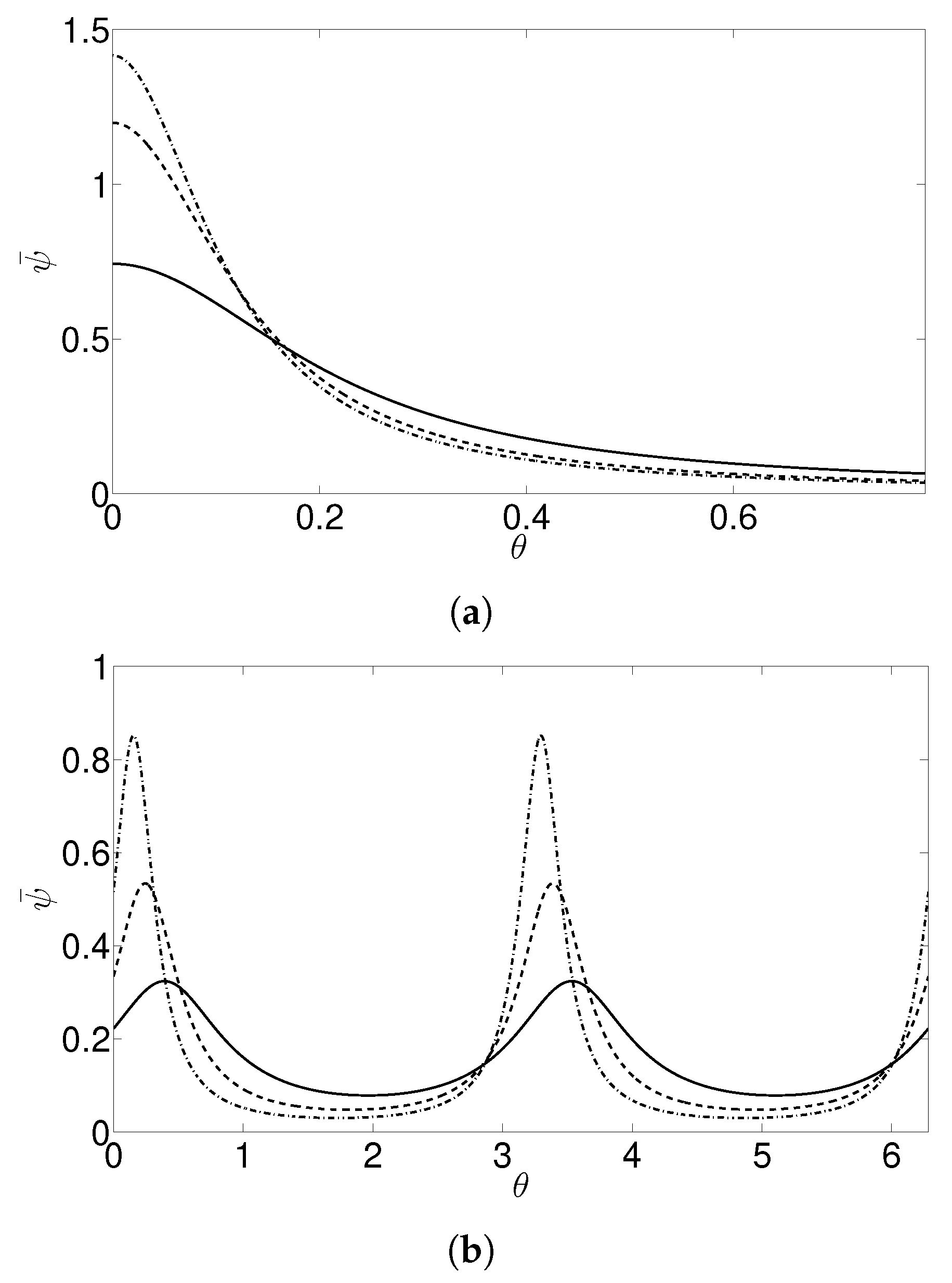
Figure 1.
(a) The radially averaged probability distribution for elongational flow for with and , denoted by the solid, dashed, and dot-dashed lines, respectively, in the upper quadrant . (b) The radially averaged distribution under shear flow, with .
Figure 1.
(a) The radially averaged probability distribution for elongational flow for with and , denoted by the solid, dashed, and dot-dashed lines, respectively, in the upper quadrant . (b) The radially averaged distribution under shear flow, with .

Figure 2.
Numerical solution for the radius of gyration plotted against the non-dimensional elongation rate for the FENE-P (dashed lines) and FENE (solid lines) for (a) , (b) , and (c) . Circular markers indicate the exact analytic solution, where it exists.
Figure 2.
Numerical solution for the radius of gyration plotted against the non-dimensional elongation rate for the FENE-P (dashed lines) and FENE (solid lines) for (a) , (b) , and (c) . Circular markers indicate the exact analytic solution, where it exists.

Figure 3.
Numerical solution for the radius of gyration plotted against the non-dimensional shear rate for the FENE-P (dashed lines) and FENE (solid lines) models for (a) , (b) , and (c) .
Figure 3.
Numerical solution for the radius of gyration plotted against the non-dimensional shear rate for the FENE-P (dashed lines) and FENE (solid lines) models for (a) , (b) , and (c) .

Figure 4.
The probability density function for the full nonlinear FENE solution with and for (a) and (b) .
Figure 4.
The probability density function for the full nonlinear FENE solution with and for (a) and (b) .

Figure 5.
The probability density function for the full nonlinear FENE solution with for and with (a) and (b) .
Figure 5.
The probability density function for the full nonlinear FENE solution with for and with (a) and (b) .

Figure 6.
The mean horizontal extension scaled by the infinitely dilute case against (a) and (b) from simulations that include the mean-field term. The results are given for denoted by the solid, dashed and dotted lines, respectively.
Figure 6.
The mean horizontal extension scaled by the infinitely dilute case against (a) and (b) from simulations that include the mean-field term. The results are given for denoted by the solid, dashed and dotted lines, respectively.


Figure 7.
The mean horizontal extension scaled by the infinitely dilute case plotted against where the mean-field term has been set to zero. The results are given for , denoted by the solid, dashed, and dotted lines, respectively.
Figure 7.
The mean horizontal extension scaled by the infinitely dilute case plotted against where the mean-field term has been set to zero. The results are given for , denoted by the solid, dashed, and dotted lines, respectively.

Publisher’s Note: MDPI stays neutral with regard to jurisdictional claims in published maps and institutional affiliations. |
© 2021 by the authors. Licensee MDPI, Basel, Switzerland. This article is an open access article distributed under the terms and conditions of the Creative Commons Attribution (CC BY) license (https://creativecommons.org/licenses/by/4.0/).
Share and Cite
MDPI and ACS Style
Chaffin, S.; Rees, J. Semi-Dilute Dumbbells: Solutions of the Fokker–Planck Equation. J 2021, 4, 341-355. https://0-doi-org.brum.beds.ac.uk/10.3390/j4030026
AMA Style
Chaffin S, Rees J. Semi-Dilute Dumbbells: Solutions of the Fokker–Planck Equation. J. 2021; 4(3):341-355. https://0-doi-org.brum.beds.ac.uk/10.3390/j4030026
Chicago/Turabian StyleChaffin, Stephen, and Julia Rees. 2021. "Semi-Dilute Dumbbells: Solutions of the Fokker–Planck Equation" J 4, no. 3: 341-355. https://0-doi-org.brum.beds.ac.uk/10.3390/j4030026