Examination of the Performance of a Three-Phase Atmospheric Turbulence Model for Line-Source Dispersion Modeling Using Multiple Air Quality Datasets

Abstract

One of the weaknesses of current line-source models for predicting downwind concentrations from mobile sources is accounting for the dispersion of effluents. Most of the investigators in the field have taken different approaches over the last 50 years, ranging from the use of Pasquill–Gifford (P-G) dispersion curves to the use of equations based on atmospheric turbulence for point source dispersion. Madiraju and Kumar (2021) proposed a three-phase turbulence (TPT) model using the key features of mobile source dispersion that appear in the existing literature. This paper examines the performance of line-source models using an updated TPT model. The generic dispersion equations were considered from the SLINE 1.1, CALINE 4, ADMS, and SLSM models. Multiple air quality field data sets collected by other investigators near the roadways were used during this study. These include field data collected from the Idaho Falls Tracer Experiment 2008 (used as the dataset to compare with the initial model), the CALTRANS Highway 99 Tracer experiment, and the Raleigh 2006 experiment. The predicted concentrations were grouped under unstable and stable atmospheric conditions. The evaluation of the model was performed using several statistical parameters such as FB, NMSE, R², MG, VG, MSLE, and MAPE. The results indicate that the ADMS and SLINE 1.1 models perform better than CALINE4 and SLSM. SLINE 1.1 tends to overpredict for stable atmospheric conditions and underpredict for unstable atmospheric conditions. A trial test was performed to implement the TPT model in the basic line-source model (SLSM). The results indicate that the majority (FB, NMSE, R², and MSLE) of the indicators have improved and are in the satisfactory range of a good model performance level.

1. Introduction

Air quality models are useful tools for the prediction of the gaseous pollutants, aerosols, and particulate matter (PM) released from a source [1]. Many researchers and scientists have evaluated these models using the data collected from field experiments during the last several decades [2]. In 2001, Hanna et al. evaluated ADMS, AERMOD, and ISC3 dispersion models concerning non-buoyant tracer releases for point, area, and volume sources with five different field data sets. The results showed that ADMS underpredicts by about 20%, AERMOD underpredicts by about 40%, and both have a scatter factor of about two. The ADMS model’s performance is slightly better than the AERMOD performance and both perform better than ISC3, an earlier model from the USEPA [3]. In 2005, the CALINE4 and CAR-FMI dispersion models were evaluated by Levitin et al. [4] against the near road measurements using the data collected at Elimäki in southern Finland from 15 September to 30 October 1995. The results indicated that the performance of both models was better at 34 m than at 17 m. However, in most cases, the performance of both models deteriorated as the wind speed reduced (decreased) and as the wind direction approached a direction parallel to the road [4]. In 2007, the ability of CALINE4 to predict the spatial variation in the hydrocarbon concentrations downwind of a motorway was assessed, along with the accuracy of COPERT III emission functions. The results indicate that the range of the observed concentrations is higher than that of those modeled. This implies that short-term modeling will tend to underestimate higher percentile concentrations. This affects the model predictions when multiple pollutants are considered [5]. In 2009, Righi compared the ADMS urban model with an urban air quality monitoring network in Ravenna, Italy by performing a statistical and diagnostic evaluation. The results indicated that the performance of the ADMS urban model is satisfactory. However, the model tends to underpredict the concentration of air pollutants [6]. In 2013, Heist performed a model intercomparison by estimating near-road pollutant dispersion. The AERMOD, CALINE3, CALINE4, ADMS, and RLINE models were used to simulate the predicted concentrations for the Idaho Falls and Caltrans Highway 99 tracer studies. The models performed best for near-neutral conditions in both tracer studies but had mixed results under convective and stable conditions. It was also observed from the results that RLINE, ADMS, and AERMOD had produced similar results and CALINE4 produced significant scatter in the model predictions [7]. In 2017, Agharkar used CALINE4 and GAM (Generalized Additive Models) to perform a model validation and comparative performance evaluation to predict the near-road black carbon. When evaluated based on graphical screening techniques and compared using the descriptive statistics, CALINE4 and GAM exhibited R² values of 0.6928 and 0.9415, with a slope of linear regression of 0.7341 and 1.094 respectively. The overall results in this study indicated that both models showed a good agreement with the measured data [8]. From the above literature review, very few studies for mobile source modeling have been reported using multiple data sets. It is important to determine whether the models are performing well using several field studies. In early 2021, Madiraju and Kumar developed a line-source dispersion model (SLINE 1.0) incorporating the effect of wind shear near the ground level, and presented the evaluation results from the Idaho field study [9].

The literature indicates that there are several models available to predict the concentration of pollutants from mobile sources. The effect of the dilution, wind speed, turbulent diffusion, and atmospheric stability are accounted for in these models. Proper parametrization of atmospheric turbulence is important to the accuracy of the predictions. The vertical dispersion coefficient (${\sigma }_z$) is one of the critical components that affect the prediction of the downwind concentration of pollutants from the vehicular exhaust. It is important to incorporate the turbulence parameters related to the wake area created by mobile sources as well as the near field while developing a line source dispersion model near the roadway [10]. Various studies indicate that the initial vertical plume spread (${\sigma }_{z0}$) depends on the vehicular turbulence, wind velocity, width of the road, residence time, the height and width of the mobile sources within the turbulent mixing zone, and other factors [11,12]. In SLINE 1.1, the width of the mixing zone which is the initial phase in the downwind direction was estimated using Benson as the width of the roadway and an additional 3 m [13]. It was assumed that ${\sigma }_{z0}$ is constant up to 6.5 m, which is based on the summation of the width of the road 3.5 m and 3 m from the edge of the road. The spread due to the wake turbulence was considered in the calculation of the ${\sigma }_z$ in the SLINE 1.0 model by introducing the term ${\sigma }_{z0}$ to the ${\sigma }_z$ equation. The wake area created by the wind flow includes thermal, vehicular, and atmospheric turbulence effects and is considered as the transition phase. This phase is considered up to a downwind distance and is dependent on the highway vehicle types. The atmospheric turbulence has a major dominance on the plume dispersion in the dispersion phase (far away from the vehicular wake area). This TPT model is considered in the SLINE 1.0 model for highway mobile sources [9].

The current approach is similar to meta-studies reported in the medical literature. A new line-source model SLINE 1.0 and the TPT model were proposed by Madiraju and Kumar in 2021. The SLINE model incorporates wind shear near the ground, and the TPT model is updated in this paper. Thereafter, the SLINE 1.0 performance using the updated turbulence model (referred to as SLINE 1.1) was evaluated using multiple data sets, and is herein compared with the three generic models: SLSM (a Simple Line Source Model given by Wark et al., in their textbook) [14]; CALINE4 (a line source model used by USEPA before the introduction of AERMOD that is still used in California) [7]; and ADMS (available from the Cambridge Environmental Research Consultants website) used in the UK [15]. Overall, the main objective of this paper is to present the assessment of the model performance to predict downwind concentrations using SLINE 1.1, CALINE 4, ADMS, and SLSM based on an updated three-phase atmospheric turbulence model and multiple data sets. This step will help us to see if the performance of the line source has improved using the proposed three-phase parametrization of atmospheric turbulence. Additionally, the comparative analysis of SLINE 1.1 with other existing line source models is performed to identify where SLINE 1.1 stands in terms of predictability.

2. Material Methods

This section provides an overview of the line-source models, updated atmospheric turbulence model, field data, and statistical evaluation methods. It is important to assess the performance of the SLINE model using the three-phase atmospheric turbulence model as compared with the existing models. The considered existing models include CALINE4, ADMS, and SLSM, and their generic formulation is freely available in the literature. The generic mathematical formulation for these dispersion models is discussed as follows.

2.1. Line Source Models

• SLINE: This is a recently developed line-source dispersion model that incorporates the effect of wind shear (magnitude) on the dispersion of gaseous pollutants. The assumptions used in the SLINE 1.0 model are: (i) the wind direction is always perpendicular to the highway; (ii) the dispersion is of a non-fumigation type; (iii) the velocity profile with height above ground level is assumed to be the same for all downwind distances; (iv) a power-law profile is assumed for the velocity, i.e., the magnitude of the wind velocity near the ground level changes rapidly and follows a power law; (v) the eddy diffusivity profile is a conjugate of the velocity profile; and (vi) the emission rate is constant. The SLINE 1.1 model follows a TPT model which is a function of downwind distance. The expression for calculating the ground-level concentration for stable and unstable atmospheric conditions is given as Equations (1) and (2) [9]:

  $$C_{\left(x,z\right)}=\frac{q}{u_{1}Sin\theta \gamma \left(s\right)}{[\frac{2}{{\left[\frac{a u_{*} x}{U_e+b_s{u}_{*}{\left(\frac{x}{L}\right)}^{\frac{2}{3}}}+m_t \right]}^2 {\left(m-n+2\right)}^2 }]}^s\mathit{exp}\left[-\frac{2 z^{m-n+2}}{{\left[\frac{a u_{*} x}{U_e+b_s{u}_{*}{\left(\frac{x}{L}\right)}^{\frac{2}{3}}}+m_t \right]}^2 {\left(m-n+2\right)}^2 }\right]$$

  (1)

  $$C_{\left(x,z\right)}=\frac{q}{u_{1}Sin\theta \gamma \left(s\right)}{[\frac{2}{{\left[\frac{a u_{*} x \left(1+b_u \frac{u_{*}}{U_e}\frac{x}{L}\right)}{U_e}+m_t \right]}^2 {\left(m-n+2\right)}^2 }]}^s\mathit{exp}\left[-\frac{2 z^{m-n+2}}{{\left[\frac{a u_{*} x \left(1+b_u \frac{u_{*}}{U_e}\frac{x}{L}\right)}{U_e}+m_t \right]}^2 {\left(m-n+2\right)}^2 }\right]$$

  (2)

  where, C is the concentration of pollutants at a point (x, z),
  q (g/m/s) is the emission rate of pollutants,
  x (m) is the downwind distance,
  z (m) is the vertical height of the receptor above the ground,
  u (m/s) is the wind velocity at the vertical height z,
  $U_e$ (m/s) is the effective wind velocity,
  m is the exponent of the power-law velocity profile,
  n is the exponent for the eddy diffusivity profile,
  s is the stability parameter based on m and n. (s = (m + 1)/(m − n + 2)),
  θ (degrees) is the angle between the line source and the wind direction,
  $u_{*}$(m/s) is the surface friction velocity,
  L is the Monin–Obukhov length,
  a, $b_s$ and $b_u$ are the empirical coefficients,
  $m_t$ vertical spread due to mobile turbulence, and
  H is the height of the source.
  The model will be called SLINE 1.1 because the turbulence model is revised as given in Section 2.2 for this paper.
• CALINE4: This is a line-source Gaussian plume dispersion model used for regulatory purposes for predicting the concentrations of pollutants near roadways. The roadway geometry, worst-case meteorological parameters, anticipated traffic volumes, and receptor positions are the initial input parameters for the model for regulatory work. The approach followed by CALINE4 assumes (i) a homogeneous wind flow field (both vertically and horizontally), (ii) steady-state conditions, and (iii) negligible along-wind diffusion. The horizontal and vertical dispersion are adequately described as unimodal. The CALINE4 model contains improved algorithms for vertical and horizontal dispersion. However, the focus of this study is on the generic equation (see Equation (3)) of CALINE4 [16].

  $$C_{\left(x,y\right)}=\frac{q}{\pi u{\sigma }_z} \underset{y_1-y}{\overset{y_2-y}{{\displaystyle \int }}}exp(\frac{-y^2}{2{\sigma }_y^2}) dy$$

  (3)

  where, ${\sigma }_z$ and ${\sigma }_y$ are the horizontal and vertical dispersion coefficients (m), and
  $y_1$ and $y_2$ are the finite line-source endpoints in y-coordinates ($y_2$> $y_1$).
• ADMS: The Cambridge Environmental Research Consultants (CERC) developed the ADMS model. Roads are modeled as line sources with no plume rise and with modifications to account for traffic-produced turbulence, and street canyons, which is an optional feature. The vertical plume spread parameter (${\sigma }_{z_{roads}}$) is increased to consider the extra vertical turbulence produced by traffic on busy roads [17]. Similarly, an extra component is included (not for street canyons) in the lateral plume spread parameter to model the effect of lateral turbulence. The predicted concentration (C) from a finite crosswind line source of length $L_s$ is given by Equation (4) [17].

  $$C_{\left(x,y,z\right)}=\frac{q}{2\sqrt{2}\pi {\sigma }_z\left(x\right)U}\mathit{exp}\left(-\frac{{\left(z-z_p\right)}^2}{2{\sigma }_z^2}\right)\ast [\mathit{erf}\left(\frac{y+\frac{L_s}{2}}{\sqrt{2} {\sigma }_y}\right)-\mathit{erf}\left(\frac{y-\frac{L_s}{2}}{\sqrt{2} {\sigma }_y}\right)]+\mathrm{reflection} \mathrm{terms}$$

  (4)

  where, y is the lateral distance from the plume centerline (m),
  $z_p$ is the height of the plume above the ground (m), and U is the wind speed at the plume height (m/s),
• SLSM: SLSM is a simple line-source model used to calculate the concentration of the pollutant from a mobile source using basic meteorological data and source information. The concentration is uniform in the y-direction at any given downwind distance. The wind direction is considered normal to the line of emission. If the wind direction is not normal to the line of emission, then θ (the angle between the wind direction and line source) is considered, and Sinθ appears in the equation. The Sinθ is not used in the equation if the angle is less than 45 degrees. The equation is taken from the textbook by Wark et al. [14].

  $$C_{\left(x,0\right)}=\frac{2q}{{\left(2\pi \right)}^{\frac{1}{2}}{\sigma }_{z}uSin\theta }\mathit{exp}[-\frac{1}{2}{\left(\frac{H}{{\sigma }_z}\right)}^2]$$

  (5)

The four generic model formulations discussed in this section are used in this paper to simulate the predictions based on the three available data sets. The data sets used in this study are discussed in the following section. Note that the ability of a dispersion model to predict the concentrations of the air pollutants under varying conditions could only be evaluated after field measurements are taken under similarly varying conditions.

2.2. Turbulence Parametrization

In the current analysis, the SLINE 1.1 and ADMS models follow a three-phase turbulence (TPT) model that includes the initial, transition, and dispersion phases. A detailed discussion on this TPT model is provided by Madiraju and Kumar et al. [9]. We were not able to find the plume spread equations used in ADMS in the open literature. Therefore, we are using the TPT model discussed in this paper for the ADMS model.

In the initial phase, the plume spread is calculated using Equation (6) given by Chock [18] for the downwind distance up to 6.5 m.

$${\sigma }_{z0}=1.5+\frac{\left(1.5+\frac{0.5W}{u_{m}sin\varphi }\right)}{10}$$

(6)

where, W is the width of the road (m),

$u_m$ is the mean wind speed (m/s),

$\varphi$ is the wind angle concerning the road ($°$), and

${\sigma }_{z0 }$ is the initial vertical dispersion coefficient (also the abscissa of the fitted curve: to the field data).

The thermal turbulence, vehicular turbulence, and atmospheric turbulence combinedly affect the vertical spread of the plume in the transition phase. The vertical spread of the plume for stable and unstable conditions between 6.5 m and 50 m downwind distance (transition phase) for low-level sources is calculated using Equations (7) and (8), respectively, for stable and unstable atmospheric conditions. Vehicles in motion on highways create turbulence which can increase the mixing of air pollutants and ambient air in the wake area behind the vehicles. The vertical spread incorporates the additional spread ($m_t)$ due to the turbulence created by moving vehicles.

$${\sigma }_z=\frac{a u_{*}x}{U_e\left(1+b_s \frac{u_{*}}{U_e}{\left(\frac{x}{L}\right)}^{\frac{2}{3}}\right)}+m_t \mathrm{for} 6.5 \mathrm{m} \le x \le 50 \mathrm{m}$$

(7)

$${\sigma }_z=a\frac{x u_{*}}{U_e}\left(1+b_u \frac{u_{*}}{U_e}\frac{x}{L}\right)+m_t \mathrm{for} 6.5 \mathrm{m} \le x \le 50 \mathrm{m}$$

(8)

where $m_t$ is the additional spread due to the vehicles on highways to maintain the accuracy of the model-predicted concentrations. The initial formulation of $m_t$ (see Equation (9)) is revised using the expression given by Chock [18].

$$m_t=1.5+\frac{\left(1.5+\frac{0.5W}{u_{m}sin\varphi }\right)}{10}$$

(9)

In the dispersion phase (beyond 50 m downwind distance), the vertical spread of the plume for stable and unstable conditions (see Equations (10) and (11)) for low-level sources is based on theoretical considerations and experimental data and is given by Snyder et al. [19].

$${\sigma }_z=a\frac{x u_{*}}{U_e}\frac{1}{\left(1+b_s \frac{u_{*}}{U_e}{\left(\frac{x}{L}\right)}^{\frac{2}{3}}\right)}$$

(10)

$${\sigma }_z=a\frac{x u_{*}}{U_e}\left(1+b_u \frac{u_{*}}{U_e}\frac{x}{L}\right)$$

(11)

Note that the ${\sigma }_z$ in the transition and dispersion Phases will have values varying with the downwind distance.

The CALINE4 and SLSM models use Pasquill–Gifford curves to calculate the dispersion coefficients. The expressions were taken from the literature [13].

The dispersion coefficients (${\sigma }_z \mathrm{and} {\sigma }_y)$ are typically a function of downwind distance, atmospheric stability, release height, surface roughness, averaging time, and other atmospheric variables [20,21]. ${\sigma }_z$ is one of the critical components that affect the estimation of the dispersion of pollutants from the vehicular exhaust. ${\sigma }_z$ is revised as follows instead of using a Pasquill–Gifford curve for the SLINE model. The curves from Benson and Chock are based on mobile source dispersion field data [22,23]. SLINE 1.1 original curves are based on RLINE and were derived from the data from field studies (Caltrans, Raleigh 2006, and Idaho Falls in 2008). The empirical coefficients (a, b_u, and b_s) in the dispersion coefficient expressions were adjusted based on the trial-and-error method to achieve the maximum accuracy at respective atmospheric stability using the curves reported by Benson and Chock for mobile sources.

A summary of the empirical coefficients for different stability conditions for the test case used in the paper is given in

Table 1. Revised empirical coefficients for Equations (1) and (2) under different stability conditions.

Atmospheric Stability	Empirical Coefficients	Value
Unstable conditions	a	0.40
	bu	2.00
Weakly unstable conditions	a	0.75
	bu	3.50
Weakly stable conditions	a	0.58
	bs	2.00
Stable conditions	a	0.55
	bs	3.00

.

The model predictions are simulated using the best fit coefficients achieved for the revised expressions of SLINE 1.1. These coefficients are used in this paper to calculate the predicted concentrations computed using the SLINE 1.1 and ADMS models’ generic equations.

2.3. Field Data and Atmospheric Stability

The data considered in this study are from the experiments reported in the literature. A total of three of the data sets collected were used in the evaluation of considered dispersion models. CALTRANS99 (Data 1), Idaho Falls Tracer Experiment (Data 2), and Raleigh NO experiment (Data 3). These three were the field studies conducted to evaluate the RLINE model being incorporated in the AERMOD regulatory model by USEPA [7,19].

The CALTRANS highway 99 Tracer experiment was conducted in the 1980s in California near Highway 99 for two directions for the northbound (NB) and southbound (SB) lanes to measure SF6. The emission factors for SF6 are slightly different for the NB and SB. The line sources in NB and SB lanes were specified with a unit emission rate. Nearly 35,000 vehicles were observed in traffic daily. Since the line sources were long and the emissions were uniform along the lines, only one median receptor was modeled. The terrain is fairly flat. The samplers were placed 1 m above the ground level. The concentrations of SF6 were measured at 0 m, 32.14 m, 64.28 m, and 128.56 m downwind distance in both North and South directions [23]. In one direction, the downwind distances were represented by positive “+” and the opposite direction by negative “-” symbols (see Figure 1 and Figure 2). The wind speed ranges are observed to be 0.2 m/s–6 m/s. The atmospheric stability provided was based on Pasquill–Gifford stability categories [7].

The Idaho Falls Tracer experiment was conducted to measure SF6 in 2008 at Idaho Falls, a city in Idaho. As part of this study, two simultaneous experiments were conducted, one had a barrier downwind of the line source to represent a roadside sound wall, the other had no barrier. In this analysis, we only use the data from the no-barrier experiment to test the model concentrations for a flat roadway case. The line source in the experiment was 54 m long, the field results have been processed to represent what would have been measured had the source been infinitely long. Therefore, the input source is very long (1 km) and only one receptor is only modeled at each perpendicular downwind distance. The source is modeled with a unit emission rate because the measured emission rates are slightly different for each day. The emission rates for day 1, 2, 3, and 5 are 0.05 g/s, 0.04 g/s, 0.03 g/s, and 0.03 g/s respectively. The surface meteorology file contains only the 15 min periods where the wind direction was within 25 degrees of perpendicular to the line source. Additionally, day 4 is omitted completely, because the winds were rather erratic, and the receptor grid was not always downwind of the line source. The SF6 is measured in this field experiment for 18 m, 36 m, 48 m, 66 m, 90 m, 120 m, and 180 m downwind distances [24].

The Raleigh 2006 experiment was conducted to measure NO in Raleigh, North Carolina. The line sources were run with unit emission rates so they can be multiplied by the traffic and emission factor to determine the modeled concentration. The line source was 1 km long, and 8 lanes were used (4 lanes on each side of the median). The emission factor used was 0.5 g/vehicle/km from Venkatram 2007. The data are available for every 10 min of air [25,26].

In the current study, the performance of the considered dispersion models was determined by comparing the predicted pollutant concentrations using the model and observed pollutant concentrations from the CALTRANS99, Idaho Falls field 2008, and Raleigh data 2006.

Atmospheric stability influences the value of the plume spread in the horizontal as well as vertical direction. P-G stability is the most common method used to categorize atmospheric turbulence in the earlier literature. It is based on wind speed, incoming solar radiation (daytime), and cloud cover (nighttime). Other methods have been used to define stability class including Monin–Obukhov length, Richardson Number (R_i) [27], temperature gradient (dT/${\sigma }_z$), and standard deviation of vertical wind direction (${\sigma }_{\varnothing })$ [28]. The ranges of atmospheric stability indicators are given in

Table 2. Typical values of five stability indicators under different atmospheric conditions.

Atmospheric Stability	Pasquill Class [14]	Monin Obukhov Length (m) [27]	Richardson Number (Ri) [27]	Temperature Gradient (Degree Centigrade/100m) [14]	Standard Deviation of Vertical Wind Direction $\left({\mathit{\sigma }}_{\varnothing }\right)$ (Degree) [14]
Extremely unstable conditions	A	−2 to −3	−0.86	≤−1.9	≤12
Moderately unstable conditions	B	−4 to −5	≥−0.86 to <−0.37	−1.9 to ≤−1.7	≥10 to <12
Slightly unstable conditions	C	−12 to −15	≥−0.37 to <−0.10	−1.7 to ≤−1.5	≥7.8 to <10
Neutral conditions	D	Infinite	≥−0.10 to <0.053	−1.5 to ≤−0.5	≥5 to <7.8
Slightly stable conditions	E	35 to 75	0.053 ≤ to <0.134	−0.5 to ≤−1.5	≥2.4 to <5
Moderately stable conditions	F	8 to 35	0.134≤	1.5 to ≤4.0	<2.4
Extremely Stable	G	-	-	>4.0	-

. The atmospheric stability of the field data is categorized based on Table 2 depending upon the available information from the field study. The model predictions are simulated using the generic expressions discussed in Section 2.1 for stable and unstable atmospheric conditions and compared with the observed concentration values of the gaseous pollutants in the field. The results are discussed in Section 3.

2.4. Statistical Evaluation Methods

This paper uses Python to calculate the statistical parameters for the three independent data sets from the Idaho Falls Tracer experiment (Data 1), Caltrans Highway 99 Tracer experiment (Data 2), and Raleigh 2006 NO experiment (Data 3) [29]. The statistical parameters considered in the paper to examine the performance of the considered line-source dispersion models are discussed below:

(a)

Fractional Bias (FB): The fractional bias is a ratio between the difference of the average values and the summation of the average values of the observed and predicted concentration of pollutants, multiplied by two. It is a dimensionless number. In the ideal case, the value of FB is equal to zero. However, if its value is between −2.0 and +2.0, then the model can be referred to as better performing. If the FB value is less than −0.67, then the model is underpredicting, and if the value is less than −2.0, then the model is extremely underpredicting. If the value is higher than +0.6, then the model is overpredicting, and if the value is higher than +2.0, then the model is extremely overpredicting. The value of FB is influenced by infrequently occurring high concentration values [30,31].

$$\mathrm{FB}=2 \left( \frac{\overline{C_o}-\overline{C_p}}{\overline{C_o}+\overline{C_p}} \right)$$

(12)

where, $C_o$ is the observed concentration of pollutant, and $C_p$ is the model-predicted concentration of pollutants.

(b)

Normalized Root Mean Square Error (NMSE): The scatter in the data collected is then normalized by the product of the average values of observed and predicted concentrations of pollutants. In the ideal case, the value of NMSE is zero. A smaller NMSE value denotes that the model is better performing. NMSE values cannot be used for accessing the model predicted concentrations that are over- or underpredicted [30,32].

$$\mathrm{NMSE}=\frac{\overline{{(C_p-C_o)}^2}}{\overline{C_o} · \overline{C_p}}$$

(13)

(c)

Coefficient of Determination (R²): The coefficient of determination is the square of the correlation between the predicted and observed values. R² values range from 0 to 1. For example, an R² of 0.50 means there is 50 percent of the variance needed to predict the actual observed value [30,33].

$${\mathrm{R}}^2=1-\frac{{{\displaystyle \sum }}_{i-1}^n{\left(C_p-C_o\right)}^2}{{{\displaystyle \sum }}_{i-1}^n{\left(C_p-\overline{C_o}\right)}^2}$$

(14)

where n is the number of data points, Σ is the summation notation, and ‘i’ represents the ith value of concentration.

(d)

Geometric Mean Bias (MG): The MG value is reliable when the magnitude of the observed and predicted concentrations of the pollutants varies significantly. Extremely low values of concentrations also have strong influences on the MG value. In the ideal case, the MG value is equal to 1. If the MG value is equal to +0.5, then the model is underpredicting, and if the value is equal to +2.0, then the model is overpredicting [30,34].

$$\mathrm{MG}=\mathit{exp}(\overline{\ln C_o}-\overline{\ln C_p})$$

(15)

(e)

Geometric Variance (VG): In ideal cases, VG values are equal to 1. Similar to MG, the VG value also shows similar properties of performance measures except in the identification of over- and underprediction [30,35].

$$\mathrm{VG}=\mathit{exp}\overline{{(\ln C_o-\ln C_o)}^2}$$

(16)

(f)

Mean Squared Log Error (MSLE): Its values lie between 0 and ∞. A smaller value of MSLE indicates that the model is performing better [36].

$$\mathrm{MSLE}=\frac{1}{n}{\displaystyle \sum }_{i=0}^{n-1}{\left(lo{g}_e\left(1+C_o{}_i\right)-lo{g}_e\left(1+C_p{}_i\right)\right)}^2$$

(17)

(g)

Mean Absolute Percentage Error (MAPE): MAPE is a measure of the accuracy of the model as a percentage. MAPE can be calculated as the average absolute percent error for each predicted concentration minus the observed concentration divided by the observed concentration [37].

$$\mathrm{MAPE}=\frac{1}{n}{{\displaystyle \sum }}_{i=1}^n\left|\frac{C_o{}_i-C_p{}_i}{C_o{}_i}\right| \ast 100$$

(18)

It is always recommended to consider multiple performance measures to accurately assess models. The distribution of each variable considered determines the significance of the model performance measure. Each parameter discussed in this section was computed after obtaining the predicted model results from the SLINE, CALINE4, ADMS, and SLSM models. The formulation of each considered model and comparative analysis performed between the models are discussed in the following sections. The above statistical parameters are based on the work reported in the literature [38,39,40,41].

3. Results and Discussion

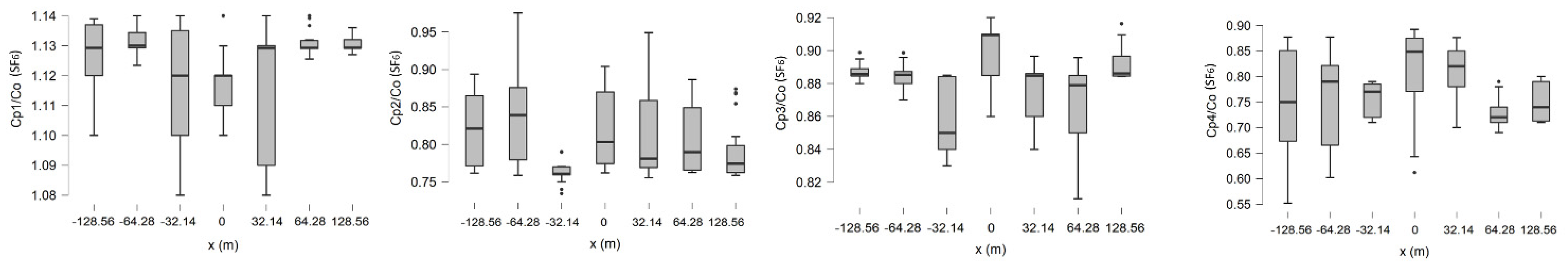
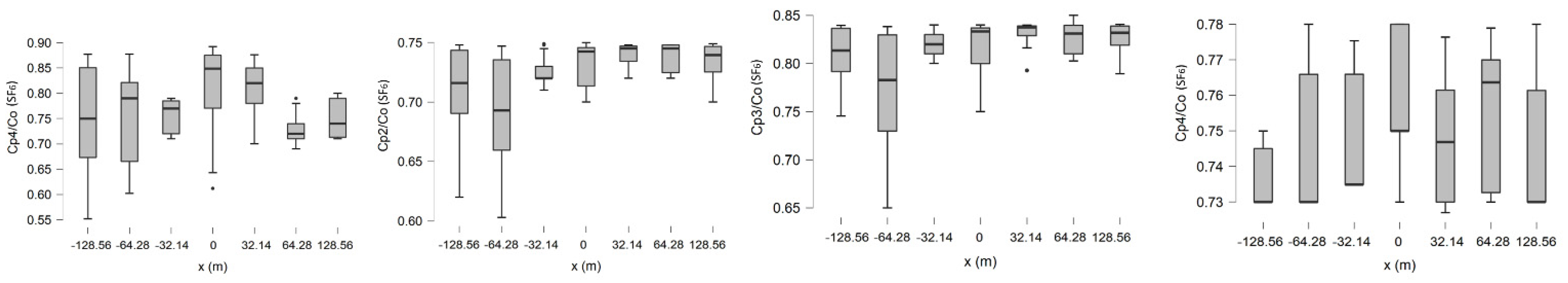
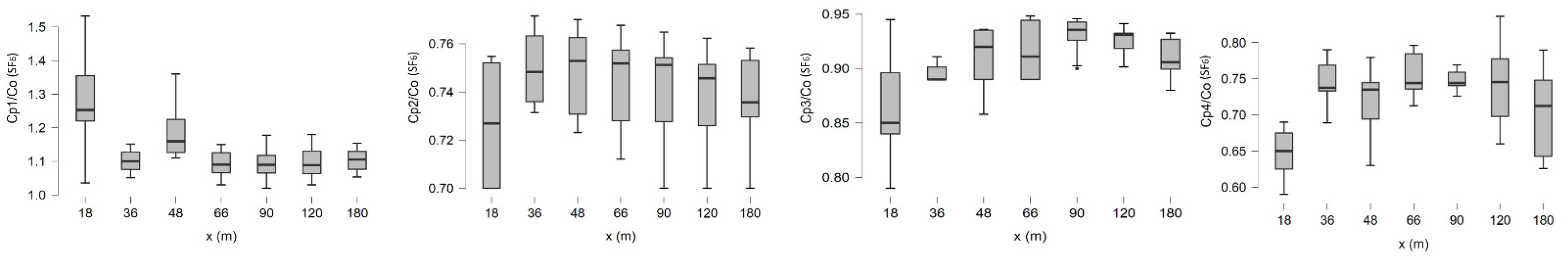
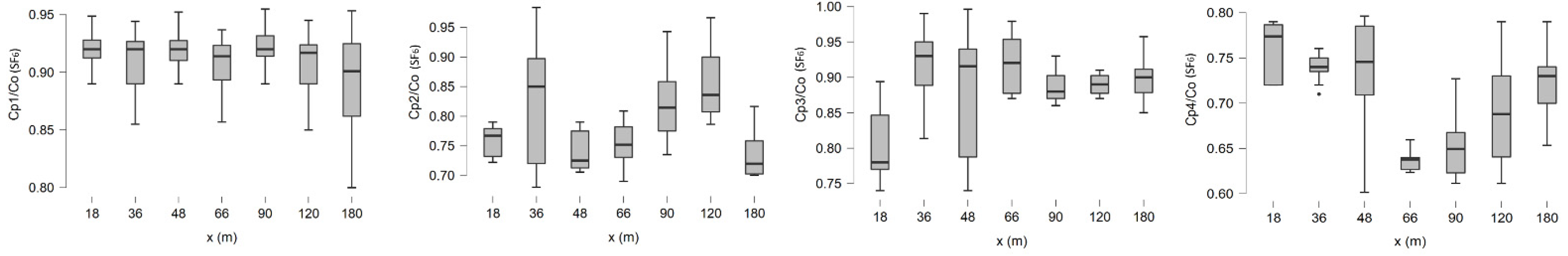
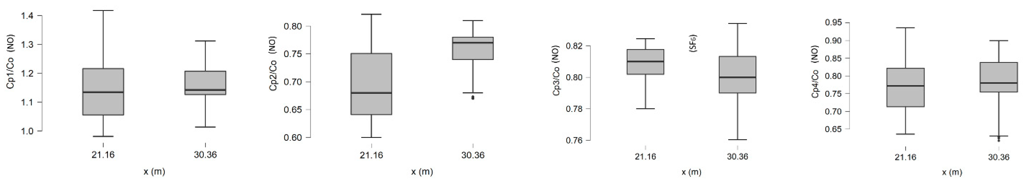
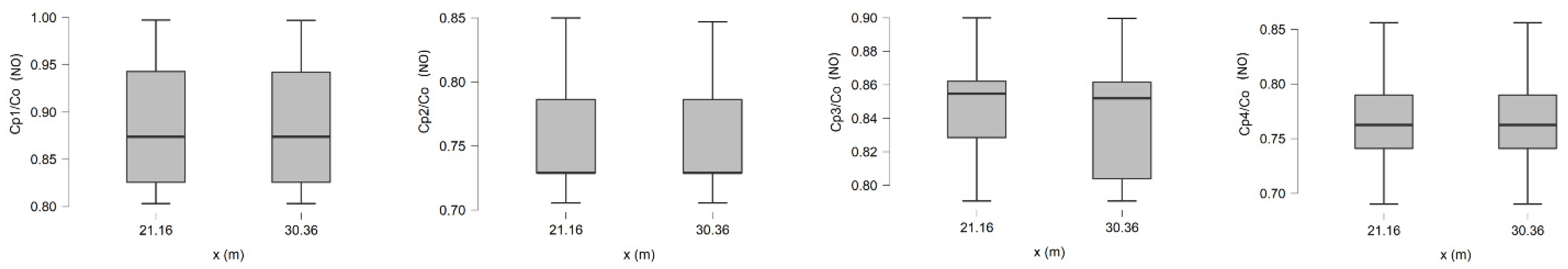
For statistical evaluation, model-predicted concentrations are evaluated against observed concentrations for different field studies. Observed concentrations are directly measured by instruments. It is important to recognize that different degrees of uncertainty are associated with different types of observed concentrations. Furthermore, it is important to define how the predicted concentrations are to be compared with the observed concentrations.

3.1. Cp/Co Plots

In the current study, the performance of the model was initially evaluated by comparing the Cp/Co values at measured downwind distances. Then, the predicted concentrations were compared with the observed concentrations using different statistical parameters. Figure 1, Figure 2, Figure 3, Figure 4, Figure 5 and Figure 6 represent the plots developed between the Cp/Co values for each model concerning the downwind distances at which the observed concentrations are measured under stable and unstable atmospheric conditions, respectively.

The Cp1, Cp2, Cp3, and Cp4 are the model-predicted concentrations of SLINE 1.1, CALINE 4, ADMS, and SLSM respectively. The plots in Figure 1 indicate that the four models show mixed results for different stability conditions and data sets. Initially, for Data 1, the SLINE 1.1 model overpredicted the concentrations under stable atmospheric conditions and underpredicted the concentrations for unstable atmospheric conditions. The ADMS model underpredicted the pollutant concentrations for stable atmospheric conditions and unstable atmospheric conditions. However, it was observed that the results of the SLSM model are significantly underpredicting for both atmospheric stability levels. It was also observed that, irrespective of the atmospheric stability condition, SLINE 1.1 and ADMS models are better performing near the highway than CALINE4 and SLSM.

Secondly, for Data 2, the Cp/Co ratios indicate that all the models considered slightly underpredicted the pollutant concentrations for stable atmospheric conditions. However, the SLINE 1.1, ADMS, and CALINE4 models performed better for stable conditions at all the downwind distances compared to the SLSM model. For unstable conditions, SLINE 1.1 and ADMS performed better than the CALINE4 and SLSM models. The CALINE4 and SLSM models were better at shorter downwind distances and had a mixed result at larger downwind distances under unstable atmospheric conditions.

Finally, for Data 3, all the models tended to slightly underpredict the pollutant concentrations for both atmospheric stability conditions. The SLINE 1.1, ADMS, and SLSM models are better-performing models under stable atmospheric conditions when compared to CALINE4. For unstable conditions, the SLINE 1.1 and ADMS models perform better than the CALINE4 and SLSM models.

3.2. Statistical Evaluation Results

The comparative analysis of model performances was then followed by statistical evaluation. The statistical indicators given by Equations (12)–(18) for four dispersion models using the three data sets as model inputs are tabulated in

Table 3. Statistical indicators/parameters computed to evaluate model performance.

	Statistical Indicator	FB	NMSE	R2	MG	VG	MSLE	MAPE
	Ideal Values	0	0	1	1	1	0	0
CALRANS99 (Data 1) Stable Conditions	SLINE 1.1	0.11	0.05	0.88	0.89	1.20	0.00258	0.12
	CALINE4	−0.26	0.37	0.75	1.44	1.35	0.00946	0.19
	ADMS	−0.14	0.10	0.86	1.24	1.22	0.00328	0.12
	SLSM	−0.26	0.35	0.73	1.41	1.48	0.01561	0.23
CALRANS99 (Data 1) Unstable Conditions	SLINE 1.1	−0.16	0.14	0.87	1.28	1.13	0.00530	0.15
	CALINE4	−0.31	0.54	0.71	1.48	1.41	0.02019	0.28
	ADMS	−0.19	0.21	0.86	1.33	1.24	0.00860	0.19
	SLSM	−0.28	0.47	0.72	1.44	1.49	0.01602	0.25
Raleigh 2006 experiment (Data 2) Stable Conditions	SLINE 1.1	0.15	0.05	0.75	0.88	1.22	0.00408	0.14
	CALINE4	−0.29	0.12	0.65	1.45	1.49	0.00172	0.26
	ADMS	−0.10	0.02	0.76	1.20	1.27	0.00206	0.09
	SLSM	−0.33	0.17	0.58	1.49	1.51	0.02117	0.28
Raleigh 2006 experiment (Data 2) Unstable Conditions	SLINE 1.1	−0.11	0.02	0.87	1.11	1.11	0.00219	0.10
	CALINE4	−0.23	0.09	0.68	1.46	1.46	0.01020	0.21
	ADMS	−0.14	0.03	0.86	1.25	1.22	0.00360	0.13
	SLSM	−0.25	0.11	0.66	1.49	1.47	0.01235	0.23
Idaho Falls 2008 (Data 3) Stable Conditions	SLINE 1.1	0.14	0.04	0.80	0.86	1.22	0.00546	0.16
	CALINE4	−0.32	0.18	0.73	1.48	1.51	0.02130	0.27
	ADMS	−0.22	0.07	0.87	1.24	1.25	0.00546	0.20
	SLSM	−0.26	0.11	0.69	1.48	1.47	0.02130	0.22
Idaho Falls 2008 (Data 3) Unstable Conditions	SLINE 1.1	−0.12	0.03	0.85	1.13	1.24	0.00382	0.12
	CALINE4	−0.26	0.10	0.74	1.42	1.48	0.01491	0.24
	ADMS	−0.17	0.04	0.83	1.29	1.33	0.00570	0.16
	SLSM	−0.26	0.11	0.74	1.41	1.49	0.01433	0.24

(FB—Fractional Bias, NMSE—Normalized Mean Square Error, R²—Coefficient of determination, MG—Geometric Mean Bias, VG—Geometric Mean-Variance, MSLE—Mean Square Logarithmic Error, MAPE—Mean Absolute Percentage Error).

. The ideal case values of each indicator are indicated in the second row of the table to assess the performance of the model.

An FB value closer to 0 indicates that the model is performing better. This indicator indicates whether the predicted values are underestimated or overestimated compared to the observed values [42]. Since the values of FB for SLINE 1.1 and ADMS are between −2.0 and +2.0, these models can be regarded as better performing. Usually, when the FB value is less than or equal to 0.3, a model is regarded as acceptable. The FB values of the models CALINE4 and SLSM were between −0.67 and −2.0 at all atmospheric conditions, showing that CALINE4 and SLSM can be regarded as underpredicting. SLINE 1.1 seems to be slightly overpredicting at stable atmospheric conditions based on the FB values. However, the model evaluation results indicate that SLINE 1.0 and ADMS have the most satisfactory values of FB when compared to the other models while evaluating all three data sets at stable and unstable atmospheric conditions. It should be noted that the FB values are based on a linear scale and represent only systematic errors which are represented in Figure 1.

The NMSE values from the results are satisfactory for all the models except for the CALINE4 and SLSM using the Caltrans data at both stable and unstable atmospheric conditions. None of the results are equal to ideal case values, but the values for SLINE 1.1 under stable conditions are suitably close. ADMS seems to be the next best-performing model when analyzed in conjunction with NMSE values. NMSE values were used in this analysis because they reflect both systematic and unsystematic errors.

The coefficient of determination (R²) assesses how strong the linear relationship is between predicted and observed concentration values. This measure is represented as a value between 0.0 and 1.0, where a value of 1.0 indicates a perfect fit, and is thus a highly reliable model for future predictions, while a value of 0.0 would indicate that the model fails to accurately model the data at all [43]. As per this analysis, the SLINE 1.1 model tends to possess a chance of 75% to 88% to accurately predict the concentration values, whereas the ADMS has a 76% to 88% chance of accurately predicting the simulations. However, CALINE4 and SLSM seem to have a chance range of 65% to 74% and 58% to 74%, respectively. Even though R² is a complex idea centered on the statistical analysis of models for data, it can be used to explain variability. The variable chance of ranges mentioned in this paragraph is based on the three considered data sets.

The MG values are based on a logarithmic scale. MG indicates systematic errors and VG indicates unsystematic errors [44]. These two statistical indicators were used in this analysis because the three data sets considered possess varying orders of magnitude. These two indicators are strongly influenced by extremely low values and provide a balanced treatment between high and low values of concentrations [29,30]. If the values are between 0.75 and 1.25, then the model is performing better. If the values are within the range of 0.50–0.75/1.25–1.50, then the model is performing better [45,46]. The MG and VG values fall in the satisfactory range for most of the models. However, none of them were equal to the ideal case value of one. In two instances, the MG and VG values for CALINE4 and SLSM exceeded the satisfactory range. This indicates that the models are performing satisfactorily as far as MG and VG values are concerned, except for CALINE4 and SLSM in some instances.

MSLE values reflect the percentage difference between the log-transformed observed and predicted concentration values. MSLE values were considered in this analysis because of their nature to treat small differences between small observed and predicted concentration values in approximately the same manner as big differences between large observed and predicted concentration values [47]. The results indicate that the values of SLINE 1.1 and ADMS are close to each other with a small difference. Similarly, CALINE4 and SLSM are close to each other with a small difference.

MAPE is the final statistical parameter used to analyze the models considered in this study. This parameter is a measure of the accuracy of the model to predict the concentration values as a percentage. MAPE was considered in this analysis in order to measure the forecast error when there are no extremes to the data [48]. CALINE4 and SLSM had the highest percentage error of 28%, whereas the highest percentage errors for SLINE 1.1 and ADMS were 16% and 20%, respectively.

3.3. Role of Quantile-Quantile (Q-Q) Plots

The predicted and observed concentrations were further assessed to see whether a model can generate a concentration distribution that is similar to the observed, especially at different concentration ranges. The Cp/Co values help to identify whether a model is underpredicting or overpredicting. The statistical indicator indicates the accuracy of the model performance. The Q-Q plots represent the similarity between the distribution of the observed and predicted values [49]. If the highest observed concentrations and model-predicted concentrations have a similar magnitude, then the model overpredicts overall, and may correctly predict the values of the highest few observed concentrations; however, this will be for the wrong reasons and at the wrong downwind distances [49]. Q-Q plots provide a visual characterization of the spread of model-predicted concentrations and observed concentrations concerning the central value [50].

Quantile-Quantile (Q-Q) plots were used in this study to visually assess the similarity in distribution between the observed concentrations and the concentrations predicted using SLINE 1.1, ADMS, CALINE 4, and SLSM. The observed and simulated concentrations using each data set were considered when drawing each plot. They were initially sorted in ascending order and plotted against the quantiles calculated from the theoretical distribution. The standardized residuals (y-axis) were the measure of the strength of the difference between the observed and predicted simulations, and the theoretical quantiles (x-axis) were the theoretically calculated percentiles [51]. The Q-Q plots for the observed data and each model simulated data were plotted (not presented in the paper). The plots indicate that all the models tend to show a similar distribution to the observed concentrations. However, while at higher concentration ranges, all the models show a slight variation in the distribution when compared to the observed concentrations.

3.4. Performance of the Basic Line-Source Model (SLSM) Using Three-Phase Turbulence Parameterization

The statistical results indicate that SLINE 1.1 performs better when compared to SLINE 1.0 with the updated three-phase atmospheric turbulence parametrization. A trial was conducted to assess the performance of the basic line-source model (SLSM) by incorporating the updated TPT model. The statistical indicators are given in

Table 4. SLSM performance using the TPT model.

Statistical Indicator	FB	NMSE	R2	MG	VG	MSLE	MAPE
Data 1 (Stable)	−0.17	0.26	0.79	1.35	1.38	0.01032	0.21
Data 1 (unstable)	−0.19	0.34	0.78	1.32	1.37	0.01125	0.22
Data 2 (Stable)	−0.22	0.13	0.69	1.36	1.39	0.01984	0.30
Data 2 (unstable)	−0.14	0.09	0.72	1.33	1.35	0.00987	0.37
Data 3 (Stable)	−0.17	0.10	0.75	1.34	1.35	0.01863	0.25
Data 3 (unstable)	−0.17	0.09	0.80	1.32	1.38	0.01104	0.20

for all three field studies used in this paper.

The comparison of results for the SLSM model given in Table 1 and Table 4 shows that there is a slight improvement in the model performance of SLSM. Improvements in the FB, NMSE, and R² values are visible. The MG and VG values have also improved. The MAPE values for Data 2 for both stable and unstable conditions increased when compared to other data sets. Note that the P–G dispersion coefficients used in the SLSM model were developed based on the work of Pasquill over 70 years ago and it is suggested that these dispersion coefficients should be replaced with the proposed turbulence parametrization.

3.5. Summary

The SLINE 1.1 model was evaluated using Cp/Co vs. downwind distance plots, statistical indicators, and the Q-Q plots. The overall model evaluation analyses from the three considered datasets shows that SLINE 1.1 is overpredicting for stable atmospheric conditions and underpredicting for unstable atmospheric conditions. The SLINE 1.1 results were observed to be closer, relatively, to the ADMS results than to CALINE4 and SLSM. The CALINE4 and SLSM models performed at a level close to the ideal values of the indicators and their overall performance was lower than SLINE 1.1 and ADMS.

Overall, it can be said that the SLINE 1.1 model is performing well using the updated atmospheric turbulence parametrization for the data sets used. The differences between the simulation results and the observed concentrations are due to the physics used during model formulation, the procedures used in measuring different field parameters, and the specifications of atmospheric stability. The researchers involved in the field experiments have done their best to simulate the mobile source emissions using tracer studies. Field data collection is subject to the resolution and sensitivity of the instrument. Model formulations, as well as instrumentation, have been improving over the last 50 years. SLINE 1.1 and the updated TPT model is an attempt to improve the physics associated with atmospheric dispersion based on our current understanding.

4. Conclusions

SLINE 1.1 incorporates wind shear near the ground and uses an updated TPT model based on the physics associated with mobile source dispersion. This study shows that the SLINE 1.1 model performs better, as compared to the results of SLINE 1.0 given by Madiraju and Kumar [9], after revising the atmospheric turbulence model. Additionally, the performance of the basic line-source SLSM model is improved when the proposed TPT model is used for dispersion calculations. This study shows that SLINE 1.1 and ADMS are better-performing models when compared to CALINE4 and SLSM.

The models used in the study incorporate improved physics, known at the time of development, related to the dispersion of effluents from mobile sources. The simulation schemes are being constantly improved over time. However, the updated three-phase atmospheric turbulence parametrization uses the current physics of mobile source dispersion and empirical coefficients based on mobile source field studies. Based on our findings, we encourage the use of the updated turbulence parametrization along with the empirical coefficients given in Table 1 with other line-source models.

It will be important to update the turbulence parametrization based on new findings reported in the field in future years. The use of the concepts of artificial intelligence (AI) for modeling mobile source dispersion is suggested based on the work of Kadiyala et al. [52].

References

1. US EPA. Air Quality Dispersion Modeling. Available online: https://www.epa.gov/scram/air-quality-dispersion-modeling (accessed on 18 October 2021).
2. Holmes, N.S.; Morawska, L. A Review of Dispersion Modelling and Its Application to the Dispersion of Particles: An Overview of Different Dispersion Models Available. Atmos. Environ. 2006, 40, 5902–5928. [Google Scholar] [CrossRef] [Green Version]
3. Hanna, S.R.; Egan, B.A.; Purdum, J.; Wagler, J. Evaluation of the ADMS, AERMOD, and ISC3 Dispersion Models with the OPTEX, Duke Forest, Kincaid, Indianapolis and Lovett Field Datasets. Int. J. Environ. Pollut. 2001, 16, 301–314. [Google Scholar] [CrossRef]
4. Levitin, J.; Härkönen, J.; Kukkonen, J.; Nikmo, J. Evaluation of the CALINE4 and CAR-FMI Models against Measurements near a Major Road. Atmos. Environ. 2005, 39, 4439–4452. [Google Scholar] [CrossRef]
5. Broderick, B.; O’Donoghue, R. Spatial Variation of Roadside C2–C6 Hydrocarbon Concentrations during Low Wind Speeds: Validation of CALINE4 and COPERT III Modelling. Transp. Res. Part D Transp. Environ. 2007, 12, 537–547. [Google Scholar] [CrossRef]
6. Righi, S.; Lucialli, P.; Pollini, E. Statistical and Diagnostic Evaluation of the ADMS-Urban Model Compared with an Urban Air Quality Monitoring Network. Atmos. Environ. 2009, 43, 3850–3857. [Google Scholar] [CrossRef]
7. Heist, D.; Isakov, V.; Perry, S.; Snyder, M.; Venkatram, A.; Hood, C.; Stocker, J.; Carruthers, D.; Arunachalam, S.; Owen, R.C. Estimating Near-Road Pollutant Dispersion: A Model Inter-Comparison. Transp. Res. Part D Transp. Environ. 2013, 25, 93–105. [Google Scholar] [CrossRef]
8. Agharkar, A. Model Validation and Comparative Performance Evaluation of MOVES/CALINE4 and Generalized Additive Models for Near-Road Black Carbon Prediction. Ph.D. Thesis, University of Cincinnati, Cincinnati, OH, USA, 2017. [Google Scholar]
9. Madiraju, S.V.H.; Kumar, A. Development and Evaluation of SLINE 1.0, a Line Source Dispersion Model for Gaseous Pollutants by Incorporating Wind Shear Near the Ground under Stable and Unstable Atmospheric Conditions. Atmosphere 2021, 12, 618. [Google Scholar] [CrossRef]
10. Yu, Y.-T. Parameterization of Vertical Dispersion Coefficient (σz) near Roadway: Vehicle Wake, Density and Types. Ph.D. Thesis, Illinois Institute of Technology, Chicago, IL, USA, 2020. [Google Scholar]
11. Macdonald, R. Theory and Objectives of Air Dispersion Modelling. Modelling Air Emissions for Compliance. MME 474A Wind Engineering. 2003, pp. 1–27. Available online: http://citeseerx.ist.psu.edu/viewdoc/download?doi=10.1.1.409.9932&rep=rep1&type=pdf (accessed on 18 October 2021).
12. Carruthers, D.; Di Sabatino, S.; Hunt, J. Urban Air Quality: Meteorological Processes. Air Pollut. Sources Stat. Health Eff. 2021, 163–191. [Google Scholar] [CrossRef]
13. Benson, P.E. Modifications to the Gaussian Vertical Dispersion Parameter, Σz, near Roadways. Atmos. Environ. 1982, 16, 1399–1405. [Google Scholar] [CrossRef]
14. Wark, K.; Warner, C.F.; Davis, W.T. Air Pollution: Its Origin and Control; Addison-Wesley: Boston, MA, USA, 1998; ISBN 0-673-99416-3. [Google Scholar]
15. CERC. Environmental Software. Available online: https://www.cerc.co.uk/environmental-software.html (accessed on 18 October 2021).
16. Johnson, R.A.; Anderson, M.; Lilly, E.; Hok, C. Implementation of CALINE4; University of Alaska-Fairbanks: Fairbanks, AK, USA, 1988. [Google Scholar]
17. Road Sources; Cambridge Environmental Research Group: Cambridge, UK, 2020; pp. 1–3.
18. Chock, D.P. General Motors Sulfate Dispersion Experiment. Bound. -Layer Meteorol. 1980, 18, 431–451. [Google Scholar] [CrossRef]
19. Snyder, M.G.; Venkatram, A.; Heist, D.K.; Perry, S.G.; Petersen, W.B.; Isakov, V. RLINE: A Line Source Dispersion Model for near-Surface Releases. Atmos. Environ. 2013, 77, 748–756. [Google Scholar] [CrossRef]
20. Thykier-Nielsen, S.; Deme, S.; Mikkelsen, T. Description of the Atmospheric Dispersion Module RIMPUFF; Riso National Laboratory: Roskilde, Denmark, 1999; pp. 1–58. [Google Scholar]
21. Kumar, A. Effects of Cross-Wind Shear on Horizontal Dispersion. J. Environ. Eng. 1986, 112, 1–11. [Google Scholar] [CrossRef]
22. Chock, D.P. A Simple Line-Source Model for Dispersion near Roadways. Atmos. Environ. 1978, 12, 823–829. [Google Scholar] [CrossRef]
23. Benson, P.E. Caline 4-A Dispersion Model for Predictiong Air Pollutant Concentrations Near Roadways; Federal Highway Administration Report FHWA/CA/TL-84/15 (NTIS PB 85 211498/AS); California State Department of Transportation: Sacramento, CA, USA, 1984. [Google Scholar]
24. Finn, D.; Clawson, K.L.; Carter, R.G.; Rich, J.D.; Eckman, R.M.; Perry, S.G.; Isakov, V.; Heist, D.K. Tracer Studies to Characterize the Effects of Roadside Noise Barriers on Near-Road Pollutant Dispersion under Varying Atmospheric Stability Conditions. Atmos. Environ. 2010, 44, 204–214. [Google Scholar] [CrossRef]
25. Venkatram, A.; Isakov, V.; Thoma, E.; Baldauf, R. Analysis of Air Quality Data near Roadways Using a Dispersion Model. Atmos. Environ. 2007, 41, 9481–9497. [Google Scholar] [CrossRef]
26. Baldauf, R.; Thoma, E.; Hays, M.; Shores, R.; Kinsey, J.; Gullett, B.; Kimbrough, S.; Isakov, V.; Long, T.; Snow, R.; et al. Traffic and Meteorological Impacts on Near-Road Air Quality: Summary of Methods and Trends from the Raleigh Near-Road Study. J. Air Waste Manag. Assoc. 2008, 58, 865–878. [Google Scholar] [CrossRef] [PubMed]
27. Leelőssy, Á.; Molnár, F.; Izsák, F.; Havasi, Á.; Lagzi, I.; Mészáros, R. Dispersion Modeling of Air Pollutants in the Atmosphere: A Review. Open Geosci. 2014, 6, 257–278. [Google Scholar] [CrossRef]
28. Scire, J.S.; Robe, F.R.; Fernau, M.E.; Yamartino, R.J. A User’s Guide for the CALMET Meteorological Model; Earth Tech LLC: Land O’Lakes, FL, USA, 2000. [Google Scholar]
29. CMAS. Community Modeling and Analysis System. Available online: https://www.cmascenter.org/download/data.cfm (accessed on 18 October 2021).
30. Model Evaluation. Available online: http://www.eng.utoledo.edu/aprg/courses/dm/hmodel.html (accessed on 10 April 2021).
31. Boylan, J.W.; Russell, A.G. PM and Light Extinction Model Performance Metrics, Goals, and Criteria for Three-Dimensional Air Quality Models. Atmos. Environ. 2006, 40, 4946–4959. [Google Scholar] [CrossRef]
32. Moursi, A.S.; El-Fishawy, N.; Djahel, S.; Shouman, M.A. An IoT Enabled System for Enhanced Air Quality Monitoring and Prediction on the Edge. Complex Intell. Syst. 2021, 7, 2923–2947. [Google Scholar] [CrossRef]
33. Chicco, D.; Warrens, M.J.; Jurman, G. The Coefficient of Determination R-Squared Is More Informative than SMAPE, MAE, MAPE, MSE and RMSE in Regression Analysis Evaluation. PeerJ Comput. Sci. 2021, 7, e623. [Google Scholar] [CrossRef]
34. Amoatey, P.; Omidvarborna, H.; Affum, H.A.; Baawain, M. Performance of AERMOD and CALPUFF Models on SO2 and NO2 Emissions for Future Health Risk Assessment in Tema Metropolis. Hum. Ecol. Risk Assess. Int. J. 2019, 25, 772–786. [Google Scholar] [CrossRef]
35. Zwain, H.M.; Nile, B.K.; Faris, A.M.; Vakili, M.; Dahlan, I. Modelling of Hydrogen Sulfide Fate and Emissions in Extended Aeration Sewage Treatment Plant Using TOXCHEM Simulations. Sci. Rep. 2020, 10, 1–11. [Google Scholar]
36. Botchkarev, A. Performance Metrics (Error Measures) in Machine Learning Regression, Forecasting and Prognostics: Properties and Typology. arXiv 2018, arXiv:1809.03006. [Google Scholar]
37. Tofallis, C. Measuring Relative Accuracy: A Better Alternative to Mean Absolute Percentage Error; Hertfordshire Business School Working Paper; University of Hertfordshire Business School, University of Hertfordshire, Hatfield: Hertfordshire, UK, 2013. [Google Scholar] [CrossRef]
38. Vijay, P.; Shiva Nagendra, S.M.; Gulia, S.; Khare, M.; Bell, M.; Namdeo, A. Performance Evaluation of UK ADMS-Urban Model and AERMOD Model to Predict the PM10 Concentration for Different Scenarios at Urban Roads in Chennai, India and Newcastle City, UK. In Urban Air Quality Monitoring, Modelling and Human Exposure Assessment; Springer Transactions in Civil and Environmental Engineering; Springer: Cham, Switzerland, 2021; pp. 169–181. ISBN 9789811555114. [Google Scholar]
39. Dėdelė, A.; Miškinytė, A. Estimation of Inter-Seasonal Differences in NO 2 Concentrations Using a Dispersion ADMS-Urban Model and Measurements. Air Qual. Atmos. Health 2015, 8, 123–133. [Google Scholar] [CrossRef]
40. Jamshidi Kalajahi, M.; Khazini, L.; Rashidi, Y.; Zeinali Heris, S. Development of Reduction Scenarios Based on Urban Emission Estimation and Dispersion of Exhaust Pollutants from Light Duty Public Transport: Case of Tabriz, Iran. Emiss. Control Sci. Technol. 2020, 6, 86–104. [Google Scholar] [CrossRef]
41. Shishegaran, A.; Saeedi, M.; Kumar, A.; Ghiasinejad, H. Prediction of Air Quality in Tehran by Developing the Nonlinear Ensemble Model. J. Clean. Prod. 2020, 259, 120825. [Google Scholar] [CrossRef]
42. Bruce, P.; Bruce, A. Practical Statistics for Data Scientists; O’Reilly Media, Inc.: Newton, MA, USA, 2017; ISBN 978-1-4919-5296-2. [Google Scholar]
43. Moriasi, D.N.; Arnold, J.G.; van Liew, M.W.; Bingner, R.L.; Harmel, R.D.; Veith, T.L. Model Evaluation Guidelines for Systematic Quantification of Accuracy in Watershed Simulations. Trans. ASABE 2007, 50, 885–900. [Google Scholar] [CrossRef]
44. Patryla, L.; Galeriua, D. Statistical Performances Measures—Models Comparison; CEA: Paris, France, 2011. [Google Scholar]
45. Patel, V.C.; Kumar, A. Evaluation of Three Air Dispersion Models: ISCST2, ISCLT2, and SCREEN2 for Mercury Emissions in an Urban Area. Environ. Monit. Assess. 1998, 53, 259–277. [Google Scholar] [CrossRef]
46. Hedges, L.V.; Olkin, I. Statistical Methods for Meta-Analysis; Academic Press: Cambridge, MA, USA, 2014; ISBN 0-08-057065-8. [Google Scholar]
47. Jauvion, G.; Cassard, T.; Quennehen, B.; Lissmyr, D. DeepPlume: Very High Resolution Real-Time Air Quality Mapping. arXiv 2020, arXiv:2002.10394. [Google Scholar]
48. Li, X.; Peng, L.; Yao, X.; Cui, S.; Hu, Y.; You, C.; Chi, T. Long Short-Term Memory Neural Network for Air Pollutant Concentration Predictions: Method Development and Evaluation. Environ. Pollut. 2017, 231, 997–1004. [Google Scholar] [CrossRef]
49. Chang, J.C.; Hanna, S.R. Technical Descriptions and User’s Guide for the BOOT Statistical Model Evaluation Software Package, Version 2.0; George Mason University and Harvard School of Public Health: Fairfax, VA, USA, 2005. [Google Scholar]
50. Kadiyala, A.; Kumar, A. Guidelines for Operational Evaluation of Air Quality Models; LAP LAMBERT Academic Publishing: Chisinau, Republic of Moldova, 2012; ISBN 978-3-8465-3277-5. [Google Scholar]
51. Goss-Sampson, M. Statistical Analysis in JASP: A Guide for Students; University of Greenwich: Amsterdam, The Netherlands, 2019. [Google Scholar] [CrossRef]
52. Kadiyala, A.; Kaur, D.; Kumar, A. Development of Hybrid Genetic-Algorithm-Based Neural Networks Using Regression Trees for Modeling Air Quality inside a Public Transportation Bus. J. Air Waste Manag. Assoc. 2013, 63, 205–218. [Google Scholar] [CrossRef] [PubMed] [Green Version]
Figure 1. Cp/Co for SF6 using CALRANS99 data (Data 1) for stable atmospheric conditions concerning the downwind distances.
J 05 00015 g001
Figure 2. Cp/Co for SF6 using CALRANS99 (Data 1) for unstable atmospheric conditions concerning the downwind distances.
J 05 00015 g002
Figure 3. Cp/Co for SF6 using the Raleigh 2006 NO experiment (Data 2) for stable atmospheric conditions concerning the downwind distances.
J 05 00015 g003
Figure 4. Cp/Co for SF6 using the Raleigh 2006 NO experiment (Data 2) for unstable atmospheric conditions concerning the downwind distances.
J 05 00015 g004
Figure 5. Cp/Co for SF6 using the Idaho Falls Tracer Experiment (Data 3) for stable atmospheric conditions concerning the downwind distances.
J 05 00015 g005
Figure 6. Cp/Co for SF6 using the Idaho Falls Tracer Experiment (Data 3) for unstable atmospheric conditions concerning the downwind distances.
J 05 00015 g006