1. Introduction
SF
6 gas is used for different HV applications, including gas-insulated switchgear (GIS, circuit breakers, switches) and gas-insulated transmission lines (GIL), because of its excellent dielectric and arc quenching properties [
1,
2]. Reference data relating to the breakdown properties of the gas in these applications have been extensively investigated and presented in the literature. Notably, it has also been widely adopted in fast-breaking plasma-closing switches for pulsed power applications because the switching element exerts a strong influence on the rising time and amplitude of the pulse [
3,
4]. These switches generally work under high voltage and current conditions and are prone to breakdown and discharge processes both thermal and non-thermal because of the extreme operational conditions and thus require a careful consideration of all discharge phases [
5] (and references there-in after).
On finding possible replacements that satisfy all necessary technical and ecological requirements for the greenhouse gas, a better understanding of the pre-breakdown and breakdown processes in SF6 is required. For the present contribution, the main focus is placed on the numerical modelling of fast-transient plasma discharge processes—streamers, their evolution in SF6 gas, and how that compares with a reference gas. A comparative numerical study has been carried out on the plasma discharge behaviour in air and SF6 in conditions relating to pulsed power applications: short separation distances, high instantaneous voltage application and non-uniform configuration, to minimize the time delay for discharge formation. The upper bounds of pressure, especially for SF6 and its influence on discharge behaviour, has also been analyzed, highlighting major physical concepts and some challenges in modelling of streamer discharges at 1 bar in the gas.
Limited literature on numerical modelling of streamers in SF6 under non-uniform fields is available, highlighting the complexity of such simulations and justifying the aims and objectives of the current study. The insights obtained from the comprehensive behaviour of an electronegative gas under high voltage stress, the streamer initiation, and propagation physics will help in identifying new gas mixtures for use in electro-technical applications.
A review of numerical modelling of streamers in SF
6 is given in
Section 2.
Section 3 provides a brief description of the mathematical model with the swarm parameters used in the present study. The obtained results for streamers in air and SF
6 at 10 and 100 kPa are reported and discussed in
Section 4, and the work is concluded in
Section 5.
2. Review of Numerical Simulations of Streamers in SF6
From an experimental point of view, previous studies have established that dielectric breakdown in SF
6 develops through formation and propagation of a stepped leader (streamer-leader transition) [
6,
7,
8,
9]. This is further highlighted by Chalmers et al. in [
10], where it was found that the development of leaders in a point to plane SF
6 gap at 500 kPa produced a streamer during the leader step development. In the recent work by Bujotzek et al. in [
11], positive and negative streamer radii and their propagation lengths have been obtained at gas pressures between 50 and 100 kPa using strong and weak non-uniform background electric fields.
From a numerical modelling point of view, limited literature exists on streamers in pure SF6 and SF6 gas mixtures.
In [
12], Morrow reviewed the dominant physical processes that affect streamer formation in SF
6 and highlighted the very high value of the electron attachment coefficient leading to a rapid formation of negative ions in the gas at atmospheric conditions. Since corona discharge formation is a time-dependent process, the effect of the high values of the attachment coefficient leading to the creation of negative ions was taken into account by evaluating the characteristic attachment time and subsequently the rate of change of electron density due to the attachment process.
One-dimensional continuity equations for electrons, cations, and anions including ionization, photoionization, attachment, recombination, and electron diffusion terms were used with the continuity equation for electrons being of the 2nd order and that of the ions, 1st order. The considered cases were for a uniform electric field with both negative and positive streamers, propagating in a 5 mm gap, and a non-uniform configuration with a 5 mm diameter needle electrode, 65 mm away from the grounded electrode. In the latter, a constant voltage of 50 kV was applied, and the discharge evolution studied for 3 ns before it stalled. The influence of a positive high voltage impulse was also studied as an applied voltage of 200 kV with a linear rise time of 15 ns enabled a longer propagation in the gap. To illustrate the re-illumination of the streamer channel and possibly stepped leaders, the current in the external circuit due to the movement of electrons and ions was computed using a modified version (with inclusion of negative ions and electron diffusion) of the Sato equation [
13]. The computed current fell as the streamer propagated and, after a certain time period, started to pulse regularly. This was, however, inconclusive as the model did not take into account background heating of the gas.
Two-dimensional representation of streamers in SF
6 at atmospheric pressure in a uniform field was studied in [
14]. Similarly, the continuity equations were used in [
14], but no photoionization was included. Instead, a background ionization was used in this model, which was implemented by introducing background charged particles (electrons and positive ions) uniformly distributed throughout the gap with the number density of 10
10–10
14 m
−3. This provided the benefit of understanding the dependence of the streamer propagation on the ionization density in front of it. A Flux Corrected Transport (FCT) technique coupled with a finite difference method for discretization was used in the solving of the higher order equations. The Poisson’s equation, which was used for obtaining the electric field, was solved using a fast Fourier transform in the z-direction and a cubic spline interpolation in the r-direction.
A neutral ionization density was introduced in the gap and an applied voltage of 50 kV was used. Both cathode and anode streamers were observed, and the maximum field enhancement was observed at the front of the streamers. More qualitative occurrences, such as the increase in the velocity as the streamer approached an electrode and the increase of negative ions as electrons attached rapidly due to a lower electric field in the bulk of SF6, were also observed.
The constant streamer radius model developed in [
15] accounts for the heating and radial expansion of the gas in the channel and describes the stepped pattern in propagation of positive streamer at 200 kPa in a sphere to plane configuration. In this work also, the continuity equations were used with an extra reaction term to describe the generation of precursor electrons ahead of the streamer front due to ionization of gas molecules by photons produced in the streamer head. An examination of the discharge current showed a series of short pulses, with each pulse resulting in an increase in gas temperature in the channel and with the most intense heating taking place at the anode. The gas heating resulted in a radial expansion of the streamer channel and decrease in the gas density inside the streamer, but this was limited by the initial streamer radius that was specified, resulting in the constant streamer radius model. With the reduction in the gas density, an increase in the reduced electric field and subsequently in the ionization integral is attained. When the ionization integral reached a specific value, the second streamer formed and propagated through the gas with lower density. The second streamer thus propagated further than the preceding one.
The studies conducted in [
16,
17,
18] report on modelling of 1D and 2D streamers in mixtures of SF
6 with air at 0.1 kPa, with N
2 at 100 kPa and 200 kPa. For the 1D implementation, the swarm parameters of SF
6 and the gas mixtures were computed by the Monte Carlo Simulation (MCS) method where only the collisions between electrons and neutral particles were considered. The implementation of the continuity equations, however, duplicates the work done in [
15]. The 2D admixture approach developed in [
17] for negative streamers was implemented in COMSOL™ Multiphysics for a non-uniform gap. The convection-diffusion equations were coupled with the Poisson’s equation, and the influence of photoionization was omitted in this work in order to simplify the model presented [
17]. Further information on the evolution of the negative streamer, the effect of the mixed gas ratio, and effect of electrode shape has been provided. In [
18], the fluid model was coupled with 47 chemical reactions, and the reason for streamer decay in SF
6/N
2 mixtures with high and low SF
6 content was assessed.
3. Simulation Model
In the present work, the continuity equations for electrons, positive ions (cations), and negative ions (anions) in space and time are solved [
19,
20], taking into account drift velocity, diffusion, ionization, attachment, recombination, and background ionization (used in place of photoionization) terms.
The subscripts
,
, and
denote electrons, cations, and anions respectively;
is the particle number density (cm
−3); µ is the mobility of the charged species (cm
2/V·s);
is the diffusion coefficient (cm
2/s);
is the electric field (kV/cm);
is the time (s);
is the Townsend’s ionization coefficient (1/cm);
is the attachment coefficient (1/cm); and
is the respective recombination coefficient (cm
3/s).
is the background ionization source used to model the photoionization processes. The logarithmic values of the charged species were used. This is useful when steep gradients are involved in the transported scalar quantity and reduces the need for artificial diffusion terms while ensuring that density of species always remain positive. Validation of the logarithmic implementation of the drift diffusion equations can be found in [
19]. The convention to use a background ionization term as opposed to a full photoionization model is already established in literature notably in [
21] where the importance of photoionization and background ionization in air and N
2-O
2 mixtures for pulsed repetitive discharges were investigated; in [
22] for N
2-O
2 mixtures comparing different streamer codes and also used as a convention for gases where the photoionization process is not well established [
14,
23].
At every time step, the electric field is also computed using Poisson’s equation for electric potential
.
where
e is the elementary charge of an electron and
represents the permittivity of vacuum.
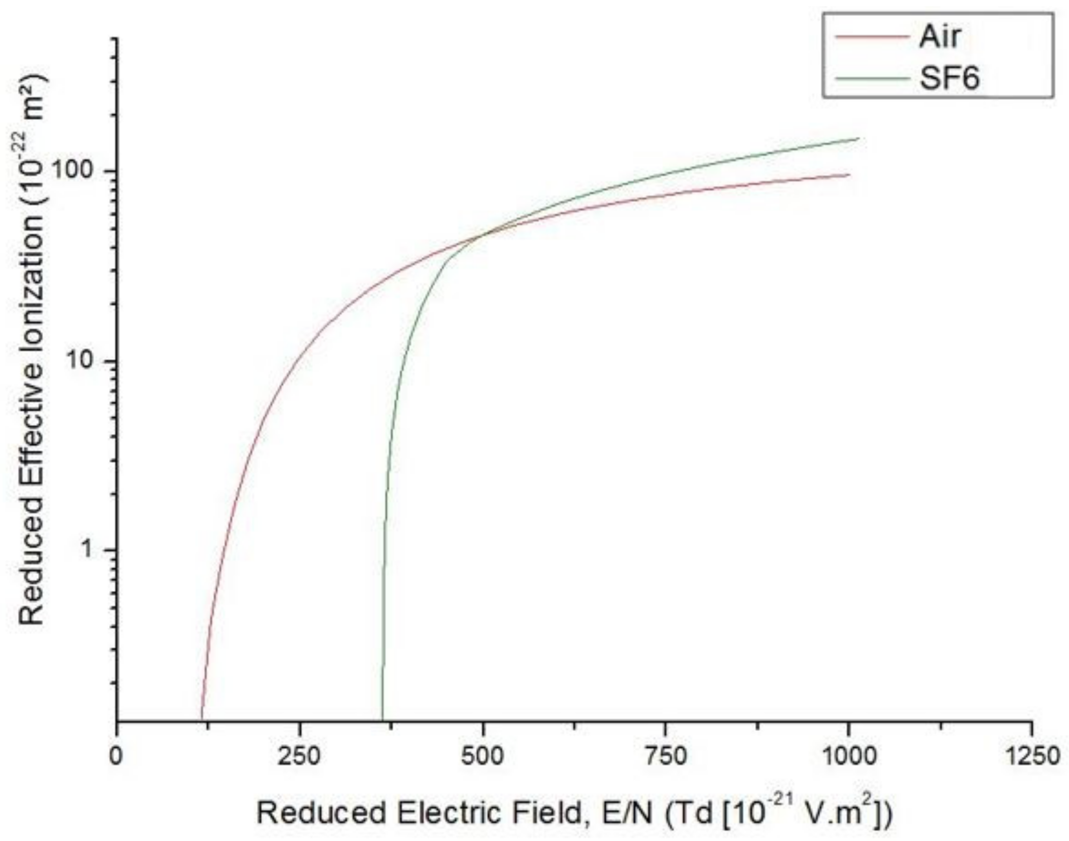
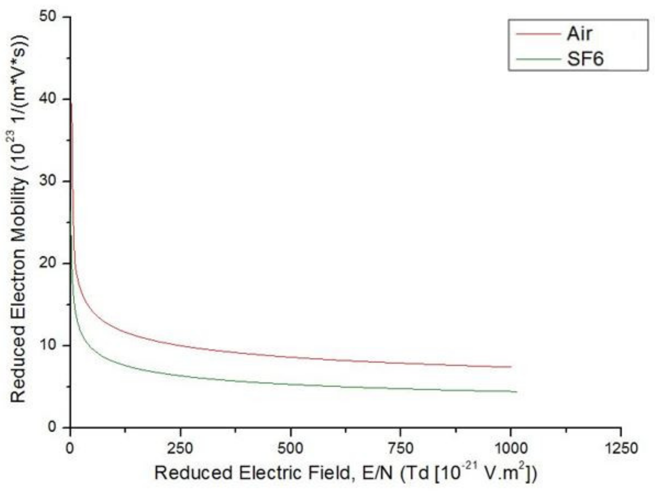
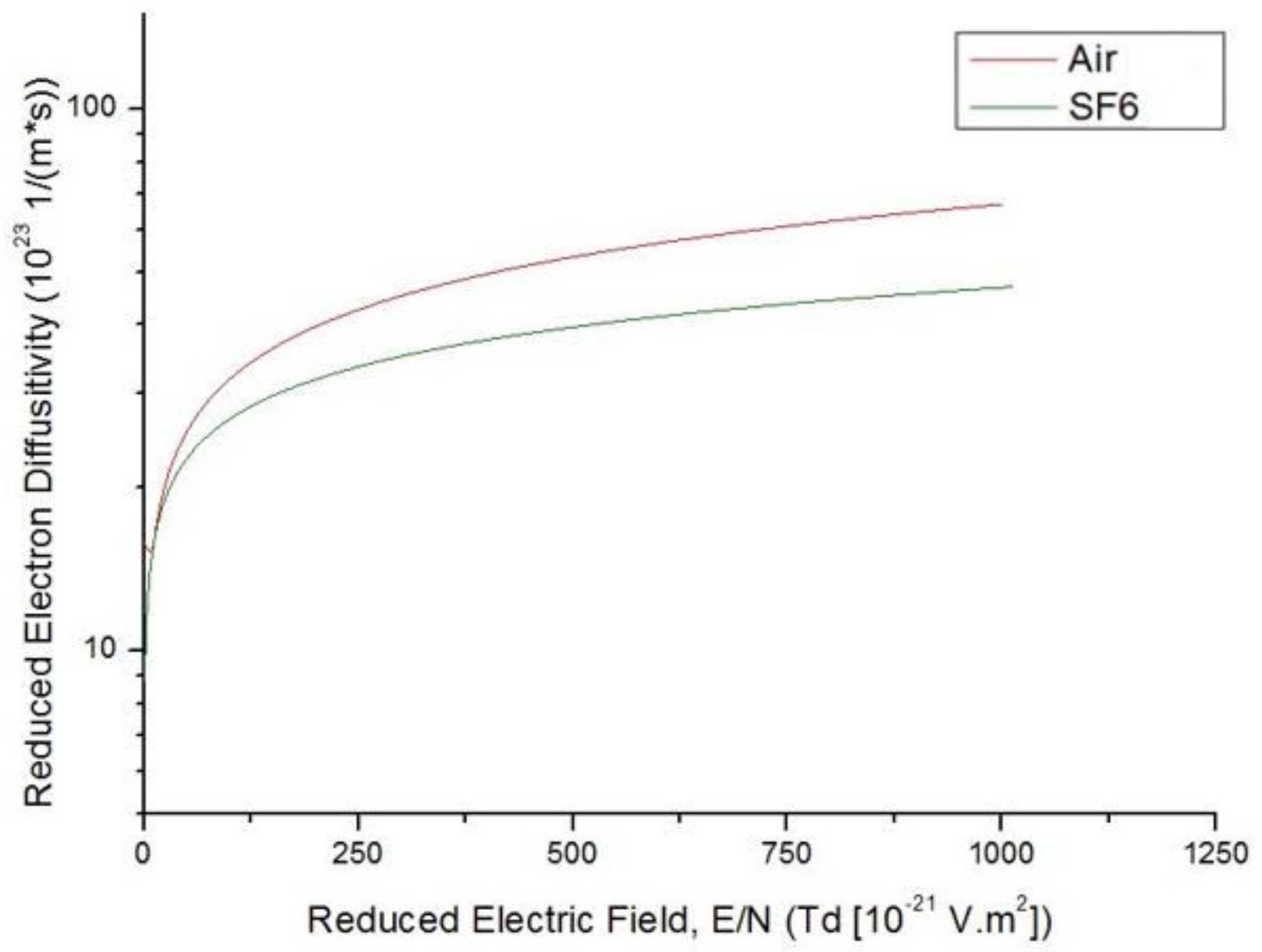
Figure 1,
Figure 2 and
Figure 3 show the reduced effective ionization
, reduced electron mobility
, and reduced electron diffusivity
as functions of the reduced electric field
for SF
6 and air. Air has been included in this analysis as a reference gas since streamer behaviour in air is well documented and understood. As shown in
Figure 1, the critical reduced electric field of SF
6 is ~362 Td as opposed to ~120 Td for air. This is the first evidence of the high attachment rate in the highly electronegative gas. The full list of parameters for the gases can be found in
Appendix C and
Appendix D.
To mimic the non-uniformity in the electric field distribution that may occur in electrical equipment due to defects, a needle—plane geometry was simulated in COMSOL™ Multiphysics [
28] with the needle (radius of curvature of 0.1 mm) serving as the high voltage electrode and the plane electrode grounded. The plasma module of COMSOL™ was used for all physics implementation and calculations. This module couples the drift-diffusion equations, heavy species transport, and electrostatic interface into an integrated multiphysics model, which allows for comprehensive analysis of plasma discharges. The discretization formulation used was finite element, log formulation (linear shape function). This uses the Galerkin method to discretize the equations.
An axisymmetric implementation of a point-plane electrode geometry in 2D space was chosen for the model. This resolves the model in cylindrical coordinates, and the initial conditions are mostly chosen in a way that the streamer develops along the symmetry axis, and therefore only the positive half axis of the model has been represented. This approach reduces the demand for computational resources in comparison to a full 3D model. However, for the post processing and output presentation, a mirror approach was adopted, and both the positive and negative half axes are shown.
As the boundary conditions used for the simulations, a voltage of positive polarity was applied to the needle electrode with the planar electrode grounded. The needle served as an outflow for the electrons and negative ions (Neumann condition) and the plane functioned as the outflow for positive ions (Neumann condition). If an electrode does not serve as an outflow for a charge specie, a Dirichlet zero condition was imposed. Open (zero flux) boundary conditions were applied to the outside planes of the computational domain.
In the present simulations, the computational domain was 5 × 7 mm (r × z) with the gap distance between the needle electrode and the plane fixed at 5 mm. The needle radius of curvature was 0.1 mm. An adaptive mesh was used to follow the propagation of the streamer in this gap. Being a finite element method simulation, triangular meshes were used for the discretization. To be able to run simulations for relatively larger gaps and computational domains, the computational domain was sub-divided. This provided the advantage of utilizing different mesh sizes depending on activity levels. In a 1.5 mm domain in the r-direction, a cell grid ranging from 2 μm to 8 μm was utilized; beyond this region, the grid expanded according to geometric progression. An adaptive mesh was used to efficiently follow the propagation of the streamer and to accurately resolve the charged layers in the vicinity of the electrodes and in areas with high gradients of charge density. The error estimation for the refinement was done with the electron reaction rate as the indicator. A minimum mesh size of 2 μm was used for this purpose. (See
Figure 4).
For the time stepping method, a BDF formula with adaptive time stepping was used. The adaptive time stepping allows the solver to take larger or smaller time steps as required to satisfy a specific tolerance. The maximum and minimum time steps were 10−9 and 10−15, respectively. The steps taken by the solver were automatically adapted within these bounds at each iteration to find a suitable solution. An output step time of 0.1 ns was used for post processing of the time dependent simulation.
4. Results and Discussion
Streamer discharges have been modelled in both air and pure SF6 gas; the needle electrode was stressed with a constant positive voltage. Development of streamers have been studied at the ambient gas temperature of 293 K and pressure values of 10 kPa and 100 kPa corresponding to the number density values of 0.2472 × 1025 m−3 and 2.472 × 1025 m−3. A background ionization in the present model is taken into account by the charge density term in Equation (1), = 1023 m−3 s−1. No Gaussian concentration of charge species was introduced for the initiation of the streamer. The gap between the point and the plane electrode was 5 mm.
For the results presented, the streamers are characterized in terms of the streamer channel length, , which is the separation between the needle electrode and the streamer head, streamer velocity , maximal field enhancement in the streamer head , streamer radius , which was obtained by measuring the radial extension of the electric field in the head of the streamer, diameter , and the electron density. Streamer velocities presented were computed when the streamer crossed the gap, and the radius/diameters were measured at axial position 2 mm.
4.1. Atmospheric Pressure (100 kPa)
Streamers in electropositive and weak electronegative gases such as N
2 and air at atmospheric pressure have been extensively studied both numerically and experimentally, however very little information on the development of streamers in highly electronegative gases such as SF
6 is available. To adequately understand the effect of the electronegativity on the streamer initiation and propagation process, a comparison has been made between the inception and propagation phases in air and SF
6 for an applied voltage of 20 kV with a maximum electric field of 610 kV/cm at the tip of the needle electrode. With a 5 mm gap, the nominal average electric field in the computational domain was obtained by dividing the applied voltage,
V, by the gap distance,
d,
, is
kV/cm. The high applied voltage and the non-uniform electrode configuration ensures that the electric field in the domain, specifically near the tip of the needle, is greater than the dielectric breakdown field for air. The average electric field
is 40 kV/cm, which is equal to or higher than the stable electric field required for streamer or leader propagation in SF
6 which is between 30–40 kV/cm [
29,
30].
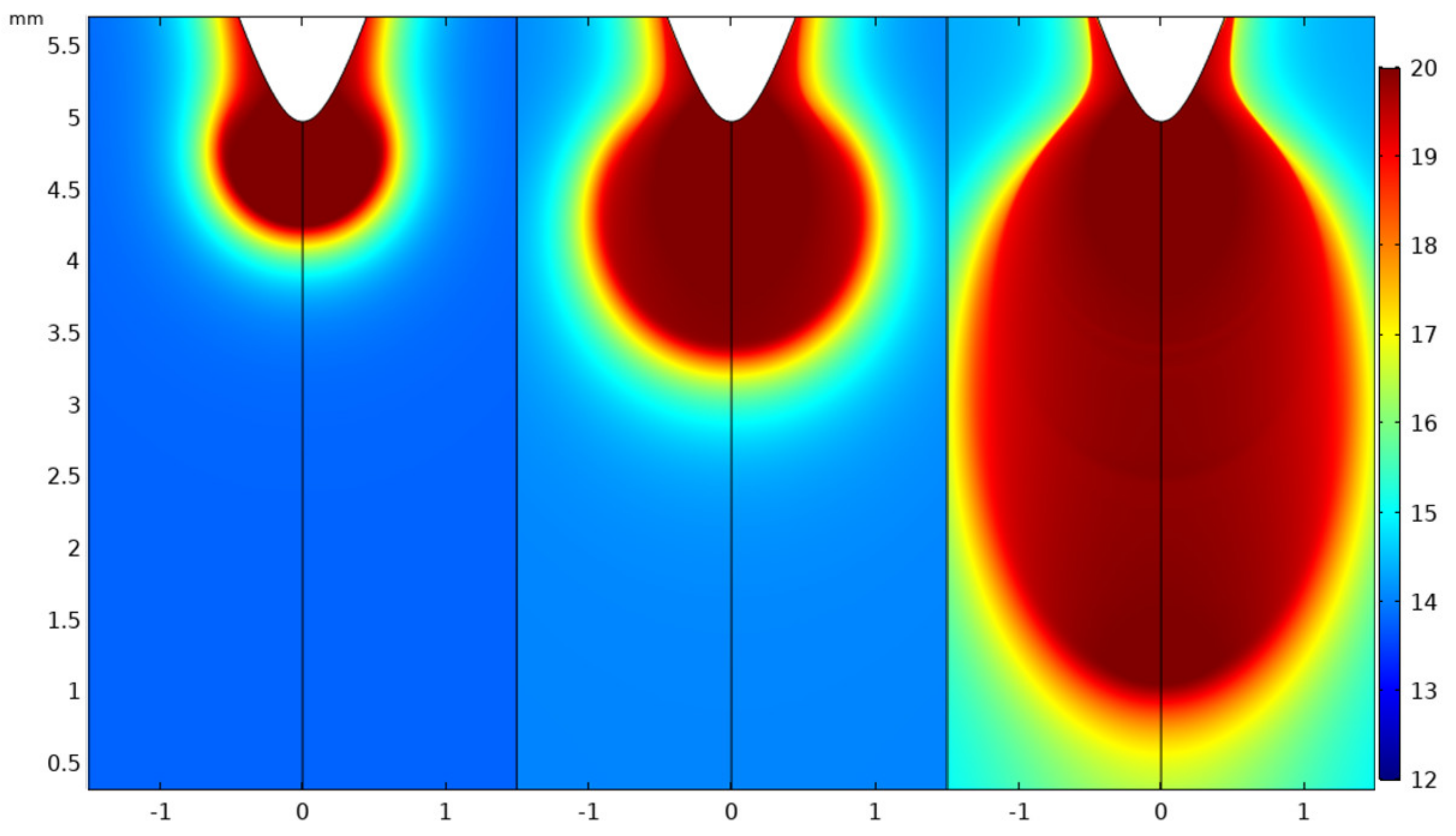
Figure 5,
Figure 6 and
Figure 7 show the 2D surface plots for the log of the electron density, the electric field distribution, and the ion densities in air at 0.5, 1 and 2 ns. The logarithmic point 1 represents 10 m
−3 while the point 20 represents 10
20 m
−3. The equivalent surface plots for SF
6 are shown in
Figure 8,
Figure 9 and
Figure 10.
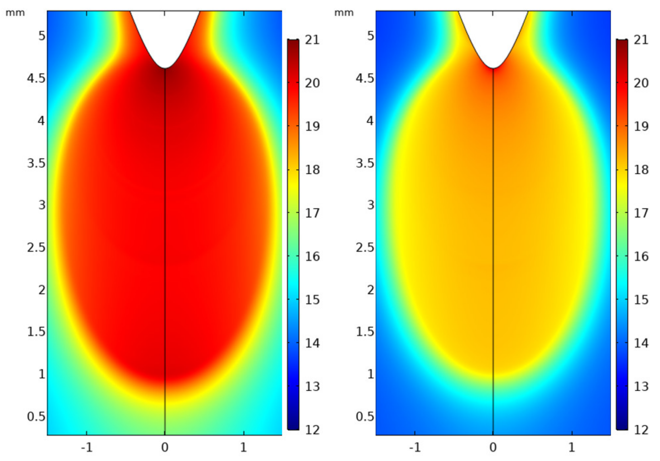
For air, the initiation and propagation of the full plasma channel is attained. In
Figure 5, the inception of the plasma front and subsequent propagation in the 5 mm air gap can be observed. The electron density in the ionized gas channel behind the propagating plasma front is ~10
20 m
−3. The different discharge phases are highlighted by the electric field diagram in
Figure 6 where the electric field achieves its peak values at the earlier times steps, then reduces when the electrostatic coupling between the streamer head and anode reduces and increases again as the streamer approaches the cathode. The head of the streamer in the stable propagation mode has an electric field of ~150 kV/cm. A comparison between the plots for the number densities of cations and anions at 2 ns (
Figure 7) show the higher concentration of positive ions to negative ions. The rate of production of positive ions is equivalent to the rate of production of electrons as both of these parameters are governed by the ionization coefficient. The rate of production of negative ions, on the other hand, is defined by the attachment coefficient which is lower in a weak electronegative gas such as air. This accounts for the difference in the ion densities.
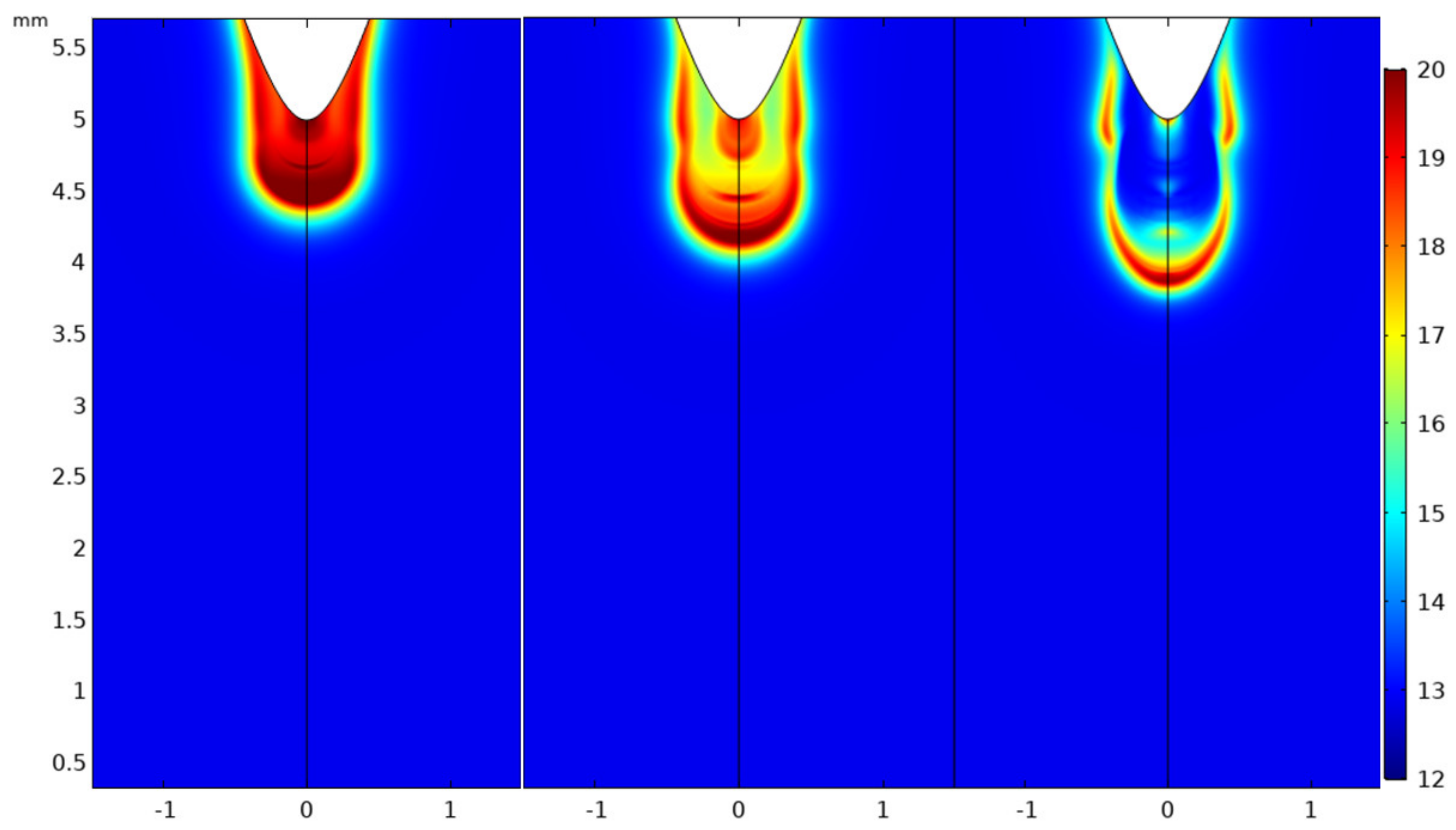
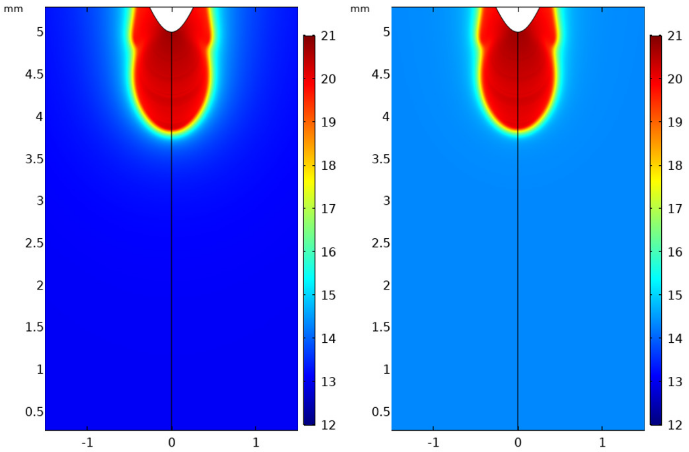
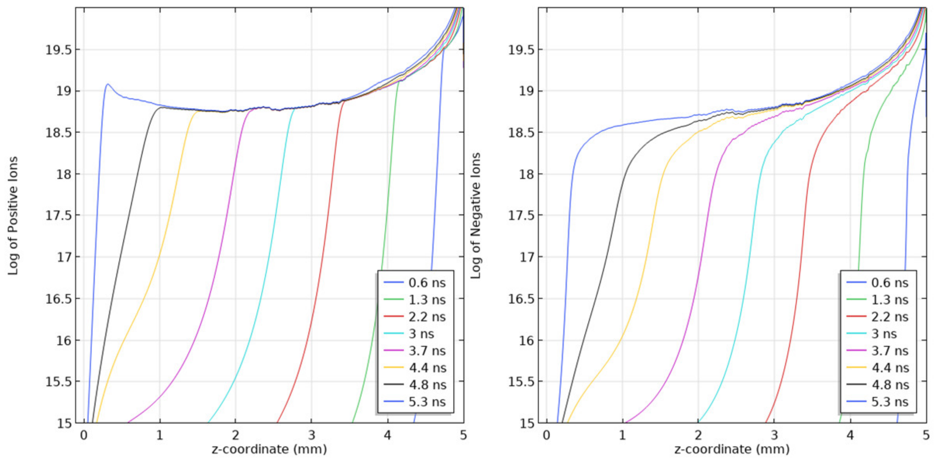
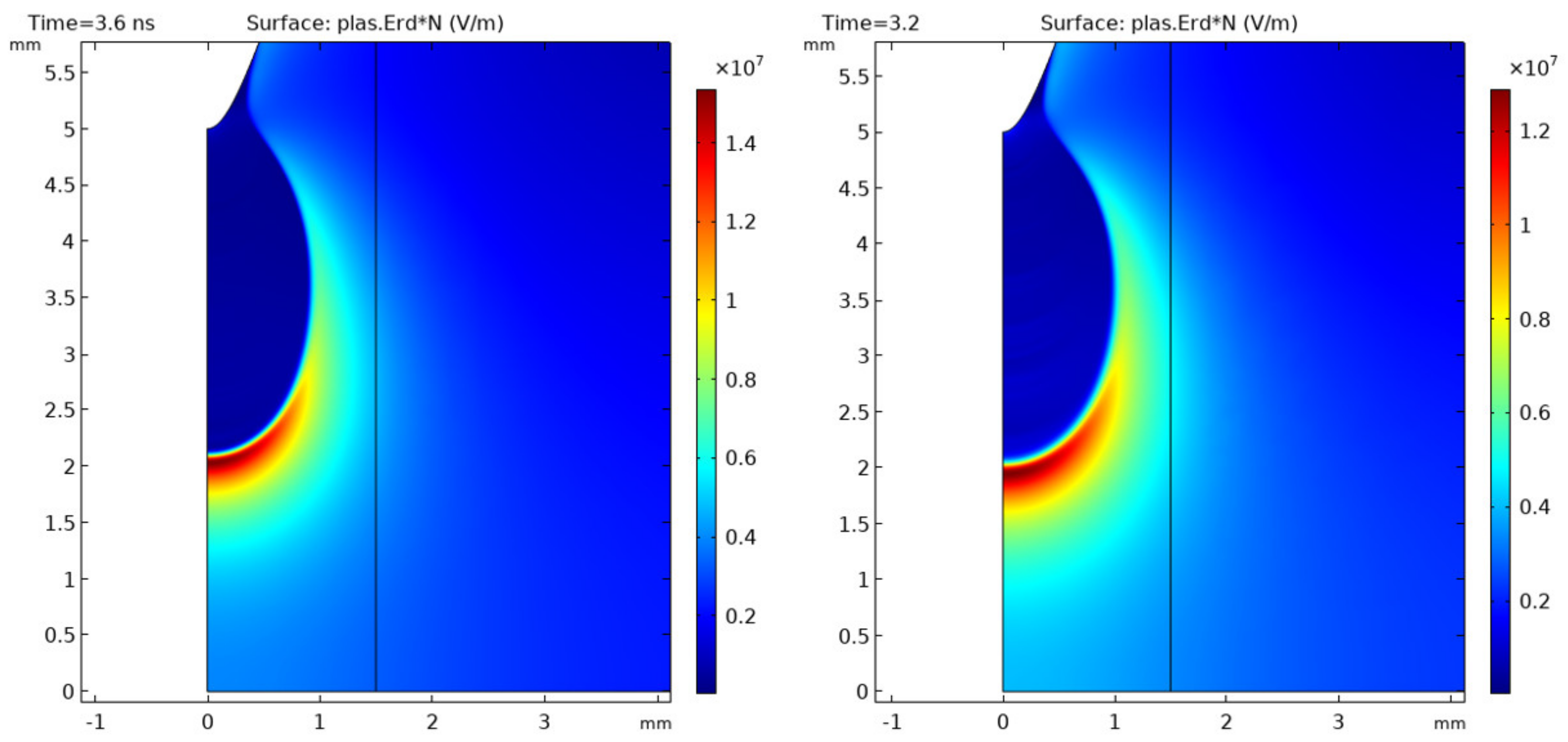
For SF
6, at the early time steps when the discharge initiates, the electric field is strengthened by the applied voltage and, consequently, the rate of ionization far exceeds the attachment rate. As the streamer propagates, the electrostatic coupling between the streamer head and the needle electrode reduces. This causes a strong affinity for attachment resulting in a high concentration of negative ions in the bulk of the streamer (See
Figure 10). In the electron density profile diagram shown in
Figure 8 (in logarithmic scale), a discontinuity can be observed between the head and the tail of the streamer resulting from the high level of attachment in the electronegative gas. In the streamer head however, due to high electric field and high ionization rate, the electron density is high and has almost the same order of magnitude as the positive ion density. The corresponding electric field plots in
Figure 9 show the enhancement of the electric field in the streamer head. A thinner streamer head with the electric field concentrated in the tip is observed as the attachment process dominates in the bulk of the streamer.
Figure 10 highlights the ion distributions in the streamer and, owing to the low drift velocities of ions and the high electron attachment rate, similar profiles are observed for both the positive and negative ions except at the tip.
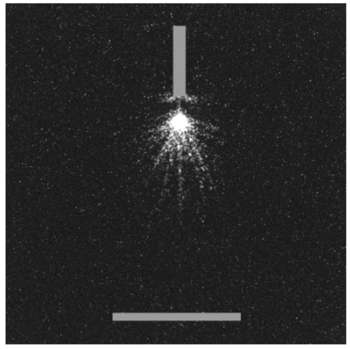
Unlike in air where the plasma front crosses the gap, in SF
6, the streamer stops propagating at about 1 mm away from the needle electrode. This can be due to the limitations of the computational model as it was shown experimentally that in SF
6 at 100 kPa and 1 cm, a leader discharge is formed, (See
Figure 11); thus, the continuity equations used in the present work cannot accurately describe the complete breakdown process. In the case of leaders, the heating of the gas should also be taken into account.
4.2. Sub-Atmospheric Pressure (10 kPa)
The simulations were repeated in air and SF
6 at the lower pressure of 10 kPa and for an applied step voltage of 5 kV with a Laplacian electric field at the tip of the needle electrode of 155 kV/cm. Similar to streamers in air at atmospheric pressure (100 kPa), the plasma front in air at 10 kPa has a radius of 1.6 mm and was observed to cross the complete inter-electrode space (5 mm gap). The streamer radius was obtained by measuring the radial extension of the electric field in the head of the streamer.
Figure 12 shows the line diagram of the electron density profile in its logarithmic form at various time steps and the corresponding electric field distribution. At steady state propagation of the streamer with an average velocity of 1.3 mm/ns, the electric field in the head of the streamer is 23 kV/cm. The electron density values attained are an order of magnitude lower than that obtained for the streamers in air at 100 kPa. Nevertheless, the general behaviour of the streamers at both pressures is the same. The flat profile of the electron density in the streamer body signifies a steady conduction path between the point electrode and the streamer head. Comparing the positive and negative ion densities, the higher ionization rate as compared to the attachment rate is highlighted in
Figure 13 where the line diagrams of the ion densities are presented in a logarithmic form for identical time steps. This correlates well with results obtained in air at 100 kPa, where a similar order of magnitude difference (2) between the positive ion density and the negative ion density was realized (see
Figure 7).
In SF
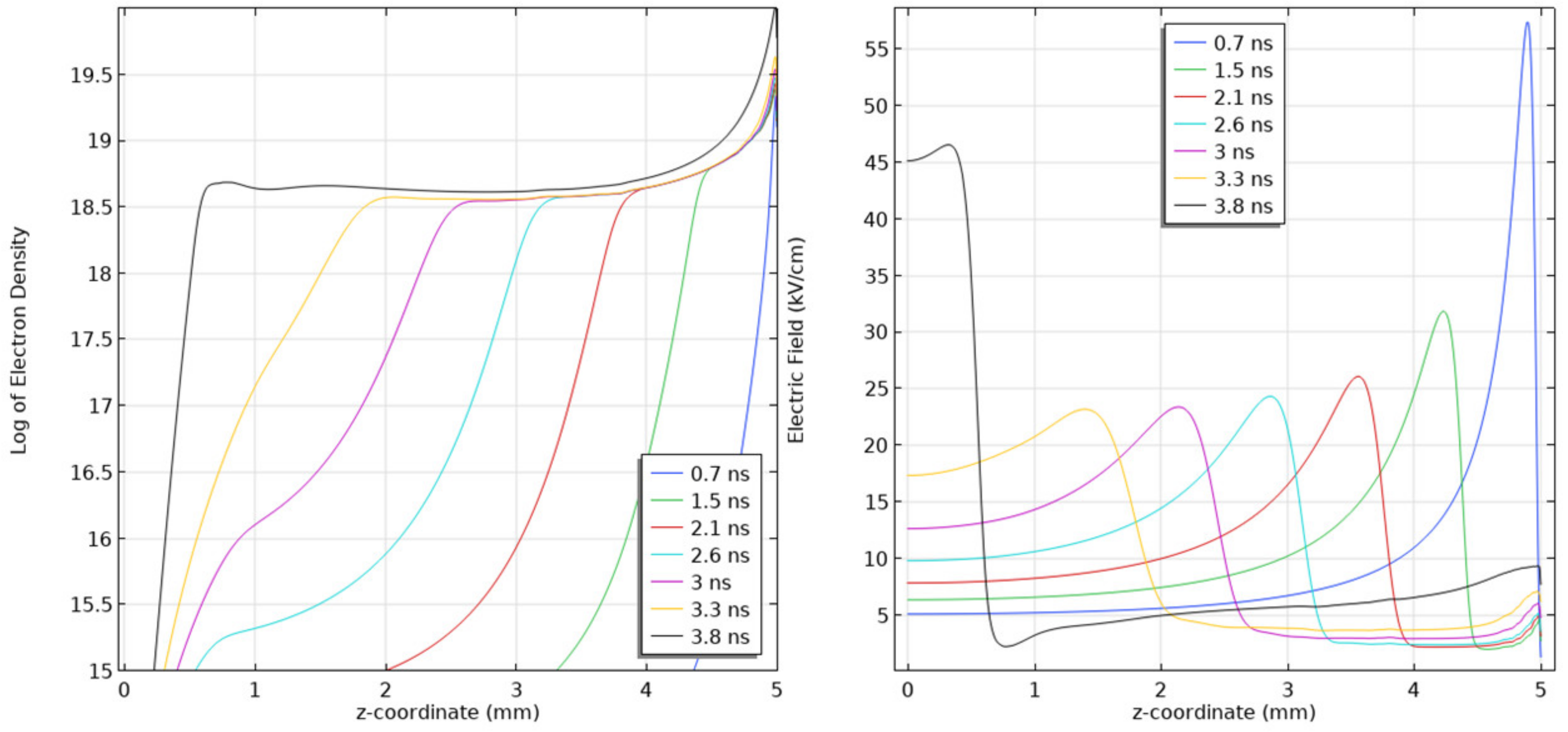
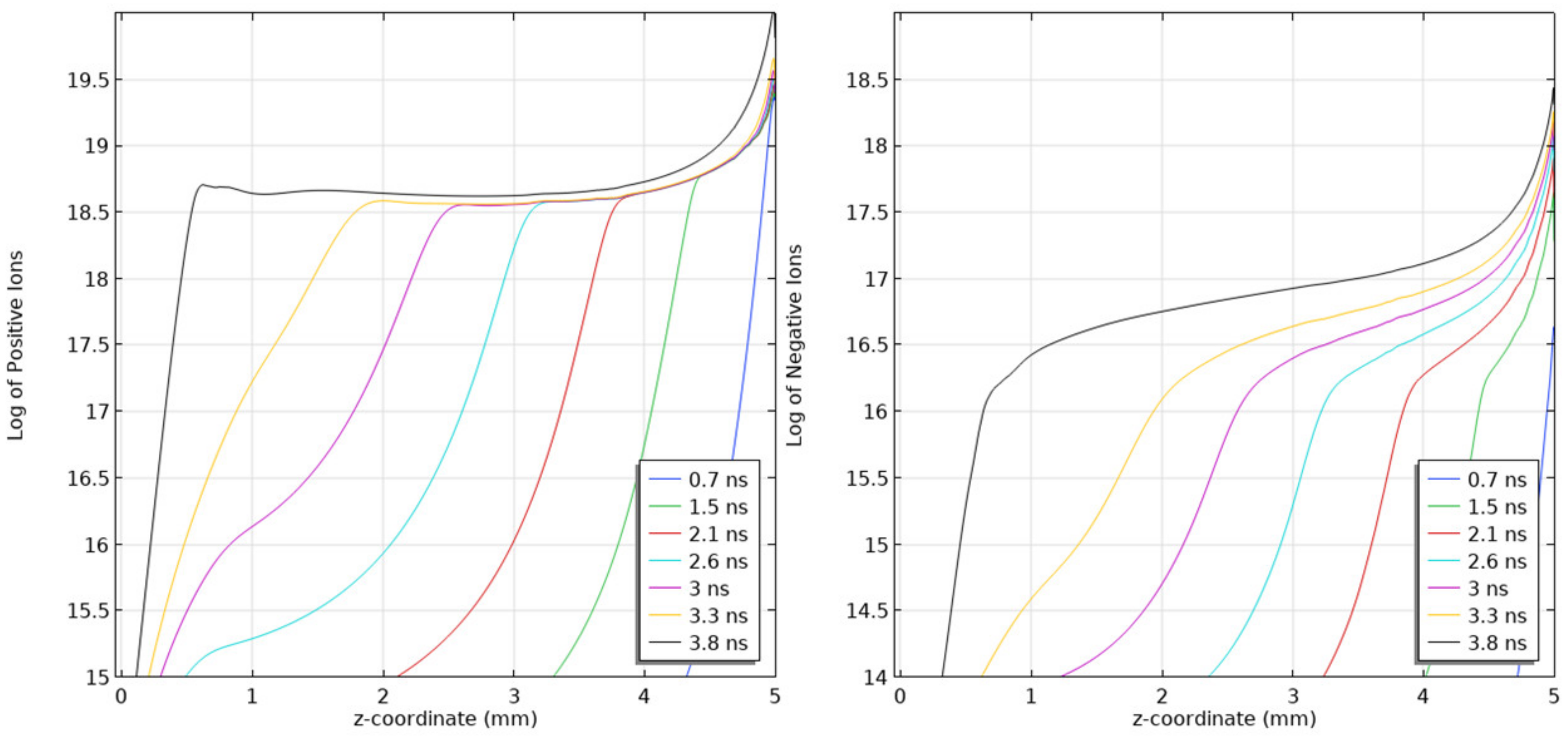
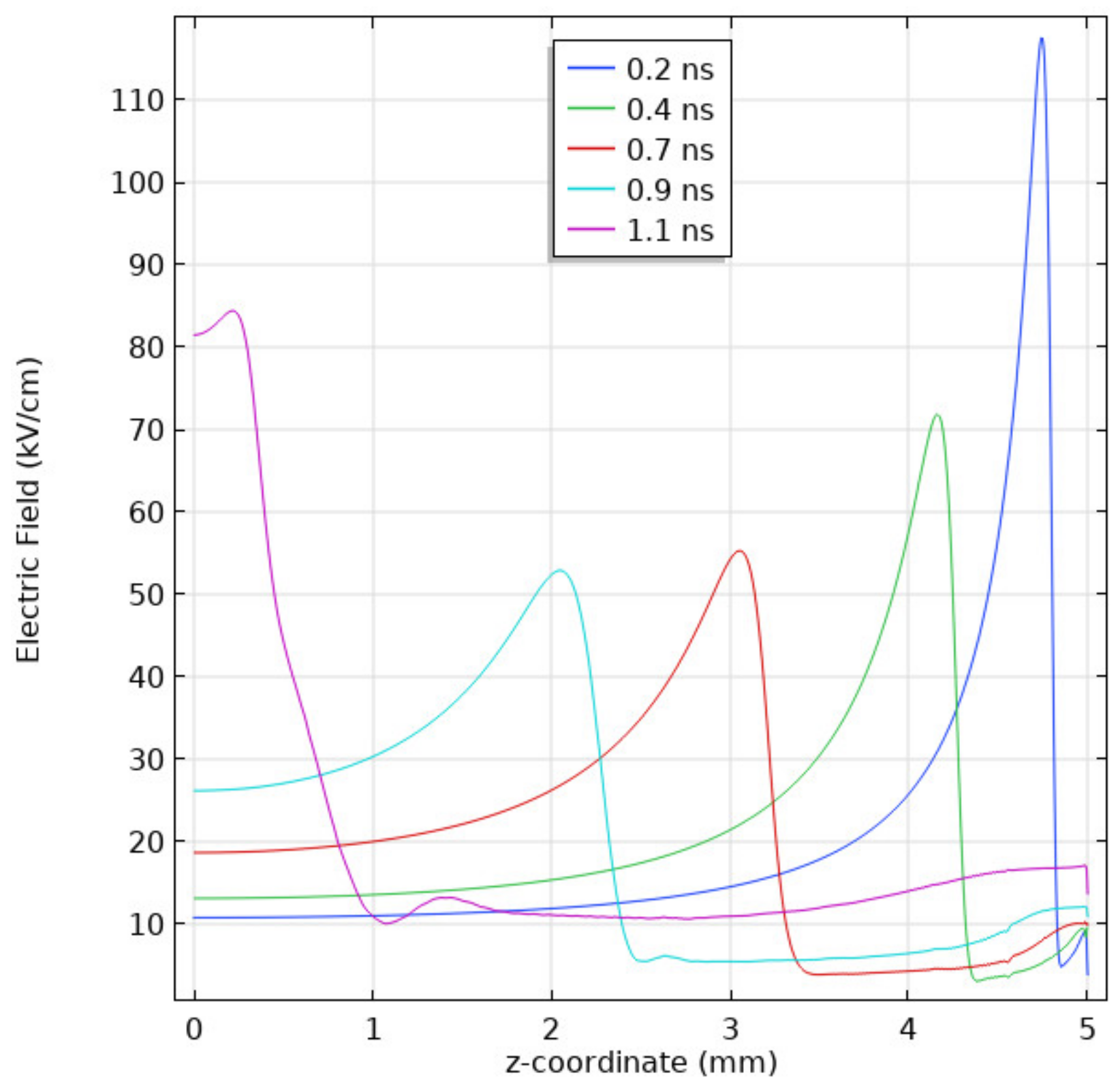
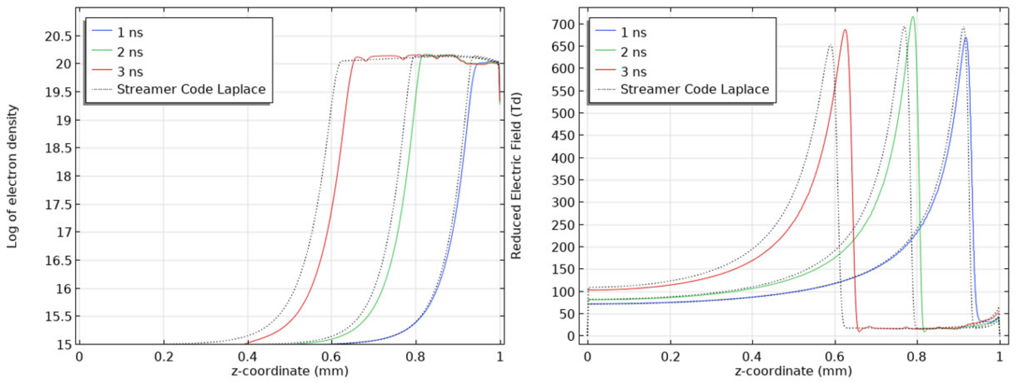
6 at pressure of 10 kPa, streamers that behave similarly to those in air were attained in the 5 mm gap when the applied voltage was 5 kV. The 1D line diagrams for the log of the electron density profiles and the electric field are shown in
Figure 14. In
Figure 15, the corresponding ion densities are presented. It was also confirmed experimentally that at gas pressure of 10 kPa, streamer discharges are obtained (see
Figure 16) as opposed to leaders observed at atmospheric pressure.
Focusing on the profile of the electron density of the streamer, the peaks represent the streamer head and the troughs represent the reduced electron density in the streamer body. As the streamer head approaches the cathode, there is a gradual increase in the electron density, a consequence of the field difference between the head and the cathode causing an increase in electron ionization. This is different from the electron density profile obtained for a streamer in air, which has a pseudo flat profile apart from when it interacts with the cathode (refer to
Figure 12).
The electric field in the streamer head in the stable propagation mode is ~27 kV/cm (
Figure 14). Thus, the reduced electric field at 10 kPa is ~1092 Td, which is well above the critical reduced electric field of 362 Td required for possible streamer propagation in SF
6 at atmospheric pressure. The high reduced electric field is required to maintain the higher ionization effect in the electronegative gas. The computed streamer velocity and radius are 0.96 mm/ns and 0.8 mm, respectively.
The ion densities in
Figure 15 show a flat profile for the positive ion density, representing the constant nature and low drift of positive ions in the streamer body as the streamer propagates towards the cathode. Similar to the electron density, there is an increase in the positive ion density close to the cathode due to increased ionization rate. The number density of negative ions, on the other hand, increases in the streamer body with each passing time step due to the high electron attachment rate. Both ion densities are of the same order of magnitude unlike in air, where the positive ion density was higher than the negative ion density (refer to
Figure 13).
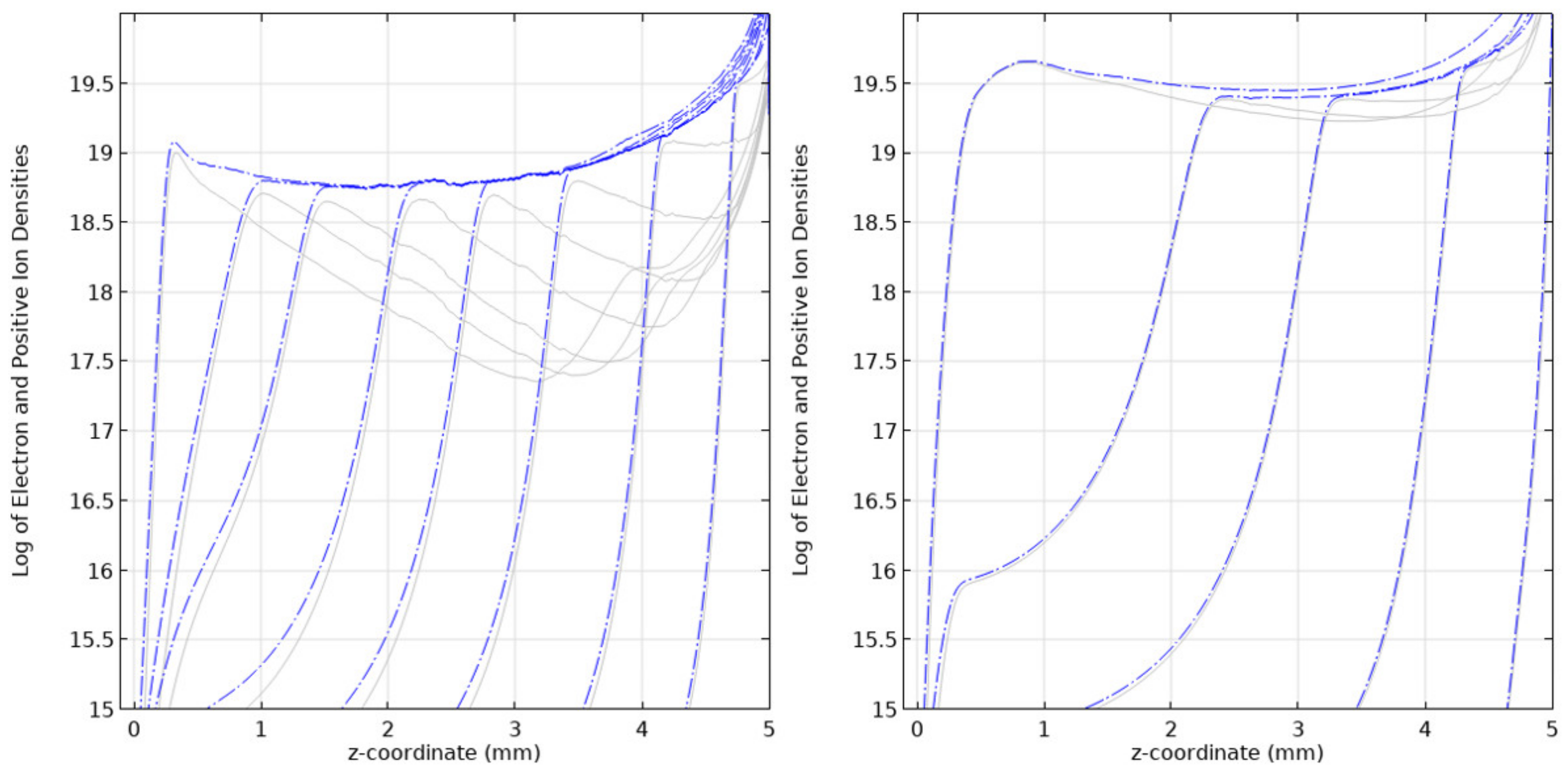
4.3. Influence of Voltage
The effect of the applied voltage on the development of streamers in SF
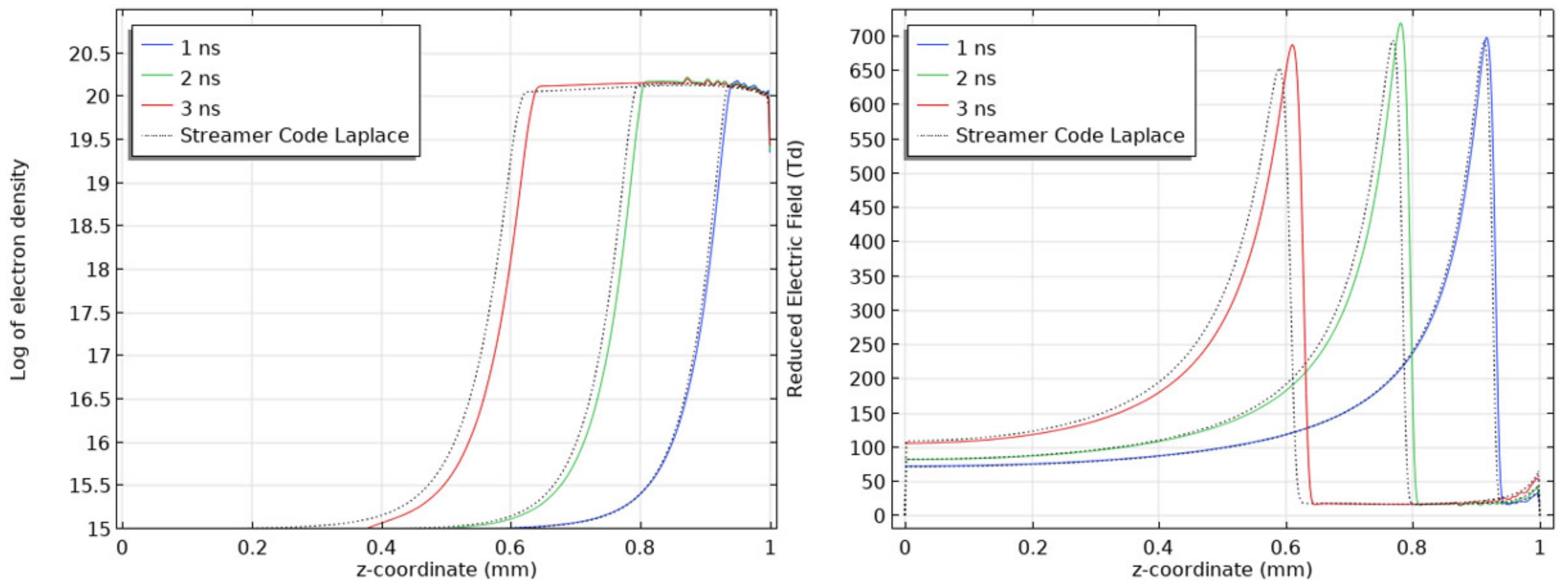
6 at a pressure of 10 kPa has been studied. The needle electrode was stressed with 5 kV and 10 kV, and the gap distance was 5 mm. As expected, the streamer forms early and travels faster with an increased applied field demonstrating a streamer velocity of 4.17 mm/ns for the applied voltage of 10 kV as opposed to 0.96 mm/ns seen in the preceding section for 5 kV. Additionally, it is interesting to discuss the electron density in the streamer body. As the voltage increases, resulting in an increase in the electric field, the rate of ionization far exceeds the rate of attachment, thus higher electron densities are realized in the streamer channel. The shape of the electron density profile resembles the flat profile characteristic of streamers in air (see
Figure 12). This is shown in
Figure 17 where the line diagrams of the positive ion density (blue dash-point lines) and electron density (solid gray lines) are plotted on the same figure for 5 kV (left) and 10 kV (right). The streamer head in this case is thicker at lower voltages than at higher ones.
Comparing the electric field in the streamer head in the steady state propagation mode, for a voltage of 5 kV, the electric field in the streamer head at steady state propagation was 27 kV/cm as opposed to 54 kV/cm for the applied voltage of 10 kV.
Figure 18 highlights this effect at 10 kPa.
The streamer radius and diameter are directly proportional to the applied voltage, and these parameters increase with an increase in the applied voltage, which is a typical dependency for streamers in other gases. This is because most of the swarm parameters used in the computational model are functions of the reduced electric field and increase as the voltage and electric field increase while the particle number density remains the same.
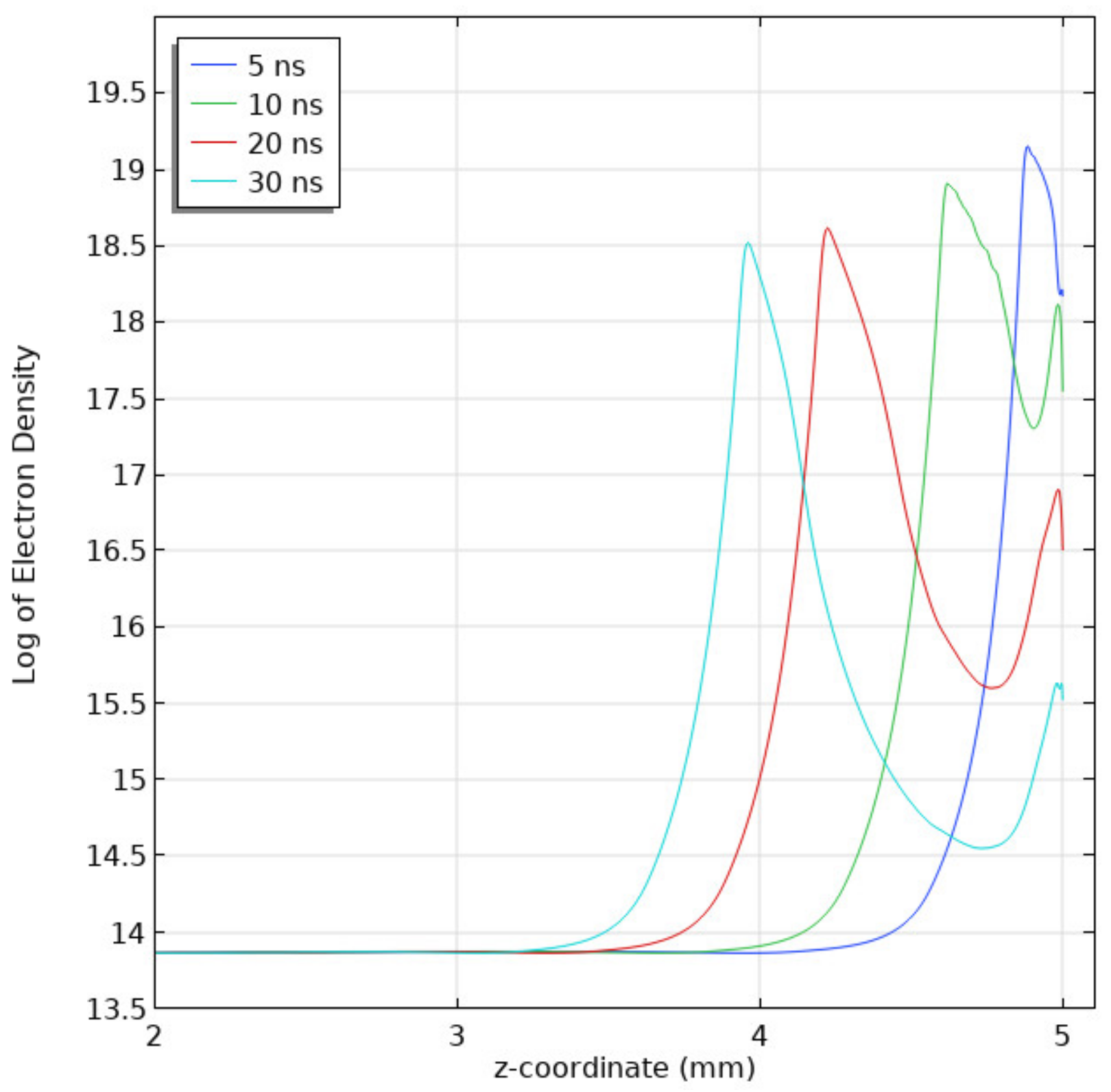
When the applied voltage was scaled accordingly to have the same reduced electric field at 10 kPa as at 100 kPa, similar numerical results were obtained for both gas pressures. Recalling, the propagation of the streamer was halted at 20 kV and 100 kPa as the electron density and subsequently conduction in the streamer channel reduced (see
Figure 8). The 1D plot of the log of the electron density at 10 kPa and for an applied voltage of 2 kV in
Figure 19 highlights this effect as the electron density in the streamer channel reduces substantially with time.
4.4. Comparison with Experimental Results
For streamer characterization, one of the most commonly used parameters is the streamer radius, especially where there is the need to compare numerical results with experimental ones. The radius of the streamer is controlled by the diffusivity of the electrons. For constant temperature, as electron diffusivity depends on the gas pressure and subsequently on the gas density, the streamer radius
is inversely proportional to the gas density as in Equation (6), [
8,
11],
where
is the pressure and
is a constant. The proportionality factor
is determined under low pressure since the radial extension reduces with increasing pressure. Different values determined using the Schlieren technique are reported in previous studies; however, the uncertainty for these experimentally obtained values of
are not provided. In [
8],
was estimated as 5 m Pa and in more recent work [
32], a proportionality factor of 2 m Pa was used in the modelling of leader propagation in uniform background field. In [
11], a confirmation for the value of C
+ is provided for both strong and weak non-uniform fields at 50 kPa and 100 kPa. For strong non-uniform electric fields, the radius of the streamer is in the range between 41 ± 6 µm and 53 ± 6 µm at 50 kPa, and 17 ± 3 µm and 22 ± 3 µm at 100 kPa. In weak non-uniform electric fields, the radius of the streamer ranged between 48 ± 7 µm and 59 ± 5 µm at 50 kPa, and 21 ± 6 µm and 28 ± 5 µm at 100 kPa. Using Equation (6) and
C+ = 2 (m·Pa) the expected radius of streamer at 50 kPa was 40 µm and 20 µm at 100 kPa. Taking only the average maximum values, the percentage error in strong non-uniform fields is 32.5% at 50 kPa and 10% at 100 kPa. For weak non-uniform fields, the percentage error is 47% at 50 kPa and 40% at 100 kPa for the average maximum radii. This is summarized in
Appendix E.
Based on the numerical simulation of streamers in SF6 at 10 kPa, a similar error analysis has been conducted. For proportionality factor C+ = 2 (m·Pa), the expected streamer radius is 0.2 mm and for C+ = 5 (m·Pa), a radius of 0.5 mm is estimated. Both values are less than the 0.8 mm (for 5 kV stress) obtained in the current simulation yielding a 30% or 60% deviation depending on the proportionality factor. Even the experimental results demonstrate an increase in the deviation as the pressure decreases, which could be a possible explanation for the difference. Another possible reason for this discrepancy could be the background ionization term used in the model instead of photoionization. However, this investigation is beyond the scope of the present work as very limited information is available on the photoionization mechanisms in SF6. For more comparable values, the applied voltage can be varied. This is, however, a trade-off between the streamer velocity and its radius.
5. Conclusions
A comprehensive behaviour of streamer discharges in a highly electronegative gas under high voltage stress has been presented and compared to a possible ecological replacement especially in electro-technical applications.
Streamer discharges in SF6 at atmospheric pressure are difficult to model numerically because of the stepped leader transition leading to the complete breakdown. In the present work, the streamer initiation is observed however the high attachment rate in the streamer channel exceeding the ionization rate leads to the reduction and eventual interruption of the conduction channel due to decreasing electron density. When this occurred, the streamer radius decreases, it halts, and an increase in the electric field in the streamer head is observed. This could be a result of the limitations of the current computational model. At low pressures, however, the streamer discharge can be characterized using the drift-diffusion partial differential equations. This modelling has been conducted for a pressure of 10 kPa with varying voltages, and the quantitative parameters have been compared to that of air at the same pressure. The results show that the electronegativity of SF6 is particularly important for the cathode directed streamer discharges as it affects the electron density in the streamer channel with both increasing and decreasing gas densities. The number densities of ions in the streamer channel are approximately equivalent with a deviation occurring in the streamer head as shown in the spatial diagrams. It was found that streamers in SF6 are characterized by smaller radii in comparison to air. The streamer radius in air obtained in the present work shows a twofold increase as compared with that in SF6. However, the velocities of streamer propagating in air and SF6 at 10 kPa are comparable with each other; ~1 mm/ns for a 5 kV applied voltage. The results presented in this paper highlight the influence of increased electronegativity on streamer discharges in gases and provide a foundation for gas mixtures with SF6 reducing streamer initiation and propagation probabilities. In future studies, the possibility of using the fluid approach to quantify the streamer to leader transition and propagation of leaders in SF6 gas will be explored. Also, the influence of field utilization factor, η on streamer dynamics in SF6 will be studied.


