Article

Fast Univariate Time Series Prediction of Solar Power for Real-Time Control of Energy Storage System

1
Smart Grid Energy Research Center, University of California, Los Angeles (UCLA), Los Angeles, CA 90095, USA
2
Senior Data Scientist, Meredith Corporation, Los Angeles, CA 90025, USA
3
Winston Chung Global Energy Center, University of California, Riverside (UCR), Riverside, CA 92507, USA
4
School of Engineering & Information Technology, University of NSW, Canberra, ACT 2610, Australia
*
Authors to whom correspondence should be addressed.
Submission received: 17 July 2018 / Revised: 13 September 2018 / Accepted: 13 September 2018 / Published: 17 September 2018

Abstract

:
In this paper, super-short-term prediction of solar power generation for applications in dynamic control of energy system has been investigated. In order to follow and satisfy the dynamics of the controller, the deployed prediction method should have a fast response time. To this end, this paper proposes fast prediction methods to provide the control system with one step ahead of solar power generation. The proposed methods are based on univariate time series prediction. That is, instead of using external data such as the weather forecast as the input of prediction algorithms, they solely rely on past values of solar power data, hence lowering the volume and acquisition time of input data. In addition, the selected algorithms are able to generate the forecast output in less than a second. The proposed methods in this paper are grounded on four well-known prediction algorithms including Autoregressive Integrated Moving Average (ARIMA), K-Nearest Neighbors (kNN), Support Vector Regression (SVR), and Random Forest (RF). The speed and accuracy of the proposed algorithms have been compared based on two different error measures, Mean Absolute Error (MAE) and Symmetric Mean Absolute Percentage Error (SMAPE). Real world data collected from the PV installation at the University of California, Riverside (UCR) are used for prediction purposes. The results show that kNN and RF have better predicting performance with respect to SMAPE and MAE criteria.

1. Introduction

1.1. Motivation and State of the Art

Renewable energy resources have been identified as essential resources to meet our energy needs; however, its capacity to replace fossil-fuel-based power generation has been hampered by its intermittency and the difficulty of predicting its availability [1]. Thus, including renewable energy as part of our energy supply requires reliable prediction of its availability for power generation. Employing prediction techniques would yield higher performance of the real time control of renewable generating plants as well as compensating devices. Moreover, forecasting algorithms are essential to improve the power quality and reliability by enabling swift mitigation of negative impacts of renewable uncertainty and intermittency [2].
The necessity of renewable energy prediction and the complexity of the prediction algorithms have motivated many researchers to develop effective and practical solutions. In particular, prediction of solar power has recently received significant attention due to new legislations encouraging the deployment of solar power plants. Solar power prediction methods can be categorized into two main groups based on the variety of parameters employed for prediction: (1) multivariate model-based methods and (2) univariate model-based methods. The multivariate methods usually estimate the solar power based on multi-input parameters, which influence solar power generation such as solar irradiance, cloudiness and clearness indices, temperature, wind speed, relative humidity, etc. On the other hand, univariate methods rely only on the current or past values of the solar power time series. Evidently, the later approach is relatively less expensive as it does not require acquiring and maintaining a weather station or other types of measurement tools. In addition, for high-speed dynamic control, which requires short-term solar power prediction, univariate methods are more effective as they do not rely on a prolonged data acquisition process. Although univariate methods only look at previous recorded data for predictions, there is usually a tradeoff between accuracy, cost and speed of the prediction methods.

1.2. Literature Review

Multivariate solar prediction methods have already been significantly investigated in the literature [3,4,5,6,7,8,9]. In the Global Energy Forecasting Competition, 12 weather variables from the European Centre for Medium-range Weather Forecasts (ECMWF) were made available to the participants to generate probabilistic forecasts of three solar farms in Australia; the proposed methods are summarized in Ref. [10]. Besides, the performances of different multivariate solar prediction methods have also been investigated and compared in several publications. Authors in Ref. [11] study eleven multivariate solar prediction methods and evaluate their performances by accuracy metrics, mean RMSE (Root Mean Square Error) confidence intervals and Box Plots describing RMSE distribution. In Ref. [12] the artificial intelligence approach is compared with a physical approach based on an error assessment criterion. Although, multivariate solar prediction methods have been noticeably studied in the literature, univariate solar prediction methods are presented only in a few publications.
Univariate model-based methods can be divided into linear models, mainly including autoregressive and autoregressive moving average models [13], and nonlinear models such as artificial neural networks [14], support vector machine with kernel trick [15], decision tree [16], wavelet-based methods [17], Markov regime switching model [18], and k-nearest neighbors (kNN) [16]. Although nonlinear models (compared to linear models) seem to be more accurate in terms of capturing the nonlinear characteristic and time varying behavior of solar power generation, these methods generally take a longer time for training/tuning parameters and easily fall into local minimum.
On the other hand, univariate prediction methods can be categorized based on the prediction horizon ranging from super-short-term (with about a minute ahead) to super-long-term prediction (with more than a year) prediction horizon in the future. Although a limited number of publications in the literature put emphasis on the super-short-term prediction timeframe, this type of prediction is useful for real time control of renewables, regulation actions and power quality enhancement. Short-term prediction methods are suitable for economic load dispatch planning or load increment/decrement decisions, and long-term prediction is normally valuable for unit commitment decisions, reserve requirement decisions, and maintenance scheduling to obtain optimal operating cost [17]. In Ref. [19], the short-term univariate prediction based on an autoregressive model and a method called the sieve bootstrap are proposed. This non-parametric method develops a full predictive density for Global Horizontal Irradiation (GHI) without imposing any parametric assumptions on the underlying distribution structure of GHI. Authors in Ref. [20] employ a hybrid solar power prediction method for super-short-time prediction. The objective of the latter paper is to predict one step-ahead solar power generation (minutely) based only on historical solar power time series data. Long–term solar prediction is investigated in Ref [17]; it develops a 1-day-ahead forecasting model based on an artificial neural network with tapped delay lines. In Ref. [21] super-long-term solar prediction is discussed; it targets the seasonality variations of solar potential for the generation of electric and thermal powers. Article [21] discussed the impact of seasonal sunlight variation on predictions of the solar-aeolic potential for power generation by developing time series models for the analysis of insolation using daily data, transformed into monthly averages.

1.3. Objective of the Study

The objective of this paper is to study the commonly used machine learning algorithms and evaluate their performance with respect to accuracy, training time, and prediction time, in order to develop a fast and super-short-term solar prediction method, based on univariate (endogenous) data, for serving as part of a real time dynamic control system. In control applications, it is important to act based on accurate, reliable and timely information. Since there is always a tradeoff between accuracy and speed, it is imperative to understand which prediction approach outperforms the others depending on the weight of accuracy and speed in different control applications.

1.4. Innovative Contribution

In this paper, four well-known algorithms including ARIMA, KNN, SVR, and RF are deployed for fast, super-short-term, univariate prediction of solar power. In order to maximize the use of available data while preserving the temporal order in time series data, the modified version of the blocked cross-validation is proposed for parameter selection. The selected prediction algorithms also allow comparing the performance of online-based algorithms with offline-based algorithms. Two of the most common error definitions are chosen to compare the accuracy performances of the super-short-term prediction algorithms. The modified version of prediction algorithms are presented for fair comparison of algorithms. Finally, the training time, and prediction time for each approach are reported to compare the speed performance of prediction algorithms.

1.5. Paper Organization

The rest of this paper is organized as follows: Section 2 describes and formulates the prediction problem, Section 3 reviews the prediction algorithms applied on our solar power generation time series. Section 4 discusses the data, preprocessing of them, and the experiment setup. Section 5 reports the result of applying the prediction algorithms and then analyzes the results. Section 6 provides the conclusion and future work.

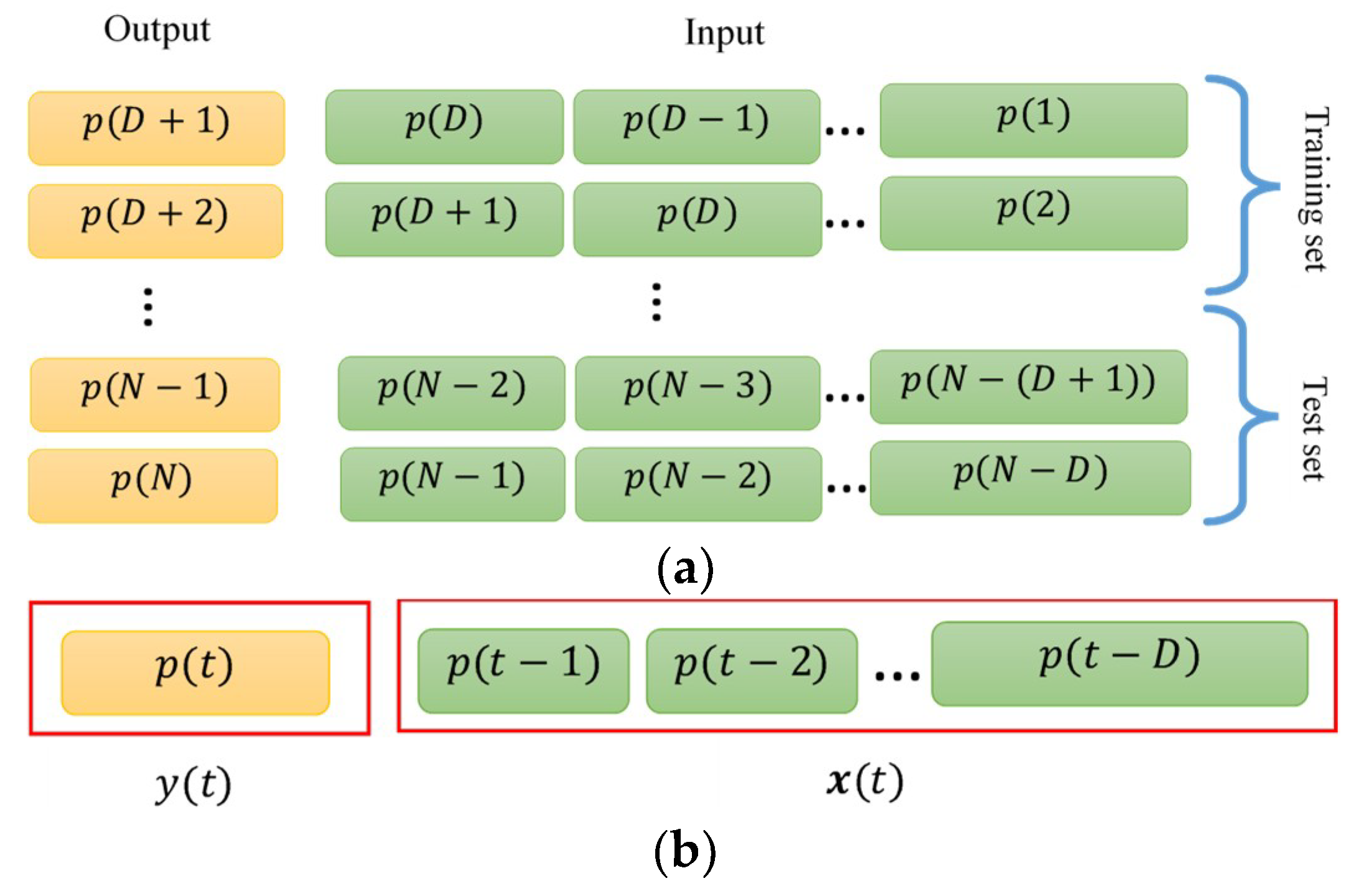
2. Problem Formulation

The objective is to predict solar power generation for the next step ahead based on the historical solar generation recorded data. Formally, it is assumed there is a function relating the predicted power and the past power:
  p ^ ( t ) = f ( p ( t 1 ) , p ( t 2 ) , )  
where p ( t ) is the actual power generated by solar panel at time t, p ^ ( t ) is the prediction of the generated power by solar panel at time t, and ( p ( t i ) ) indicates the generated power in the past at time ( t i ). The main constraint for this application is that the whole process of measurement, communication, forecasting, and control action should take less than one interval of time in order to be useful for control applications. By assuming that the whole process except forecasting takes about half an interval, the forecasting part should take well below half an interval to guarantee enough time for measurement, communication and control.
As is the usual practice in forecasting, we are interested in finding an estimation of p ( t ) that optimizes performance (or error) criterion. There are a variety of different definitions of forecasting error in the literature. To this end, two of the most common error definitions are selected and results are reported in both: Symmetric Mean Absolute Percentage Error (SMAPE) and Mean Absolute Error (MAE). The SMAPE and MAE are defined as:
  SMAPE = 1 N t s t     S t s | p ( t ) p ^ ( t ) | p ( t ) + p ^ ( t ) × 100 ,   MAE =   1 N t s t     S t s | p ( t ) p ^ ( t ) | × 100  
where N t s is the number of data points in the test set (defined below).
Let S t r = { 1 , 2 , , N t r } and S t s = { N t r + 1 , , N } be two sets of indices for the training and test sets, respectively, where N is the total number of data points, and N t r is the number of data points in the training set which makes N t s = N N t r . Later, in the parameter selection phase, parts of the training set will be treated as the validation set. The different methods used to select the validation set are further explained in the parameter selection section. In this paper, the most recent 10 percent of the data is used to evaluate the performance of the algorithm (test set). Note that the test dataset is not used in either parameter selection or training phase.

3. Applied Algorithms

The applied prediction algorithms in this paper benefit from machine learning algorithms commonly used in different disciplines [22], and also a traditional Box-Jenkins model [23]. These algorithms have also been used in other forecasting applications such as demand forecasting within smart grid framework [24]. This section summarizes the applied algorithms.

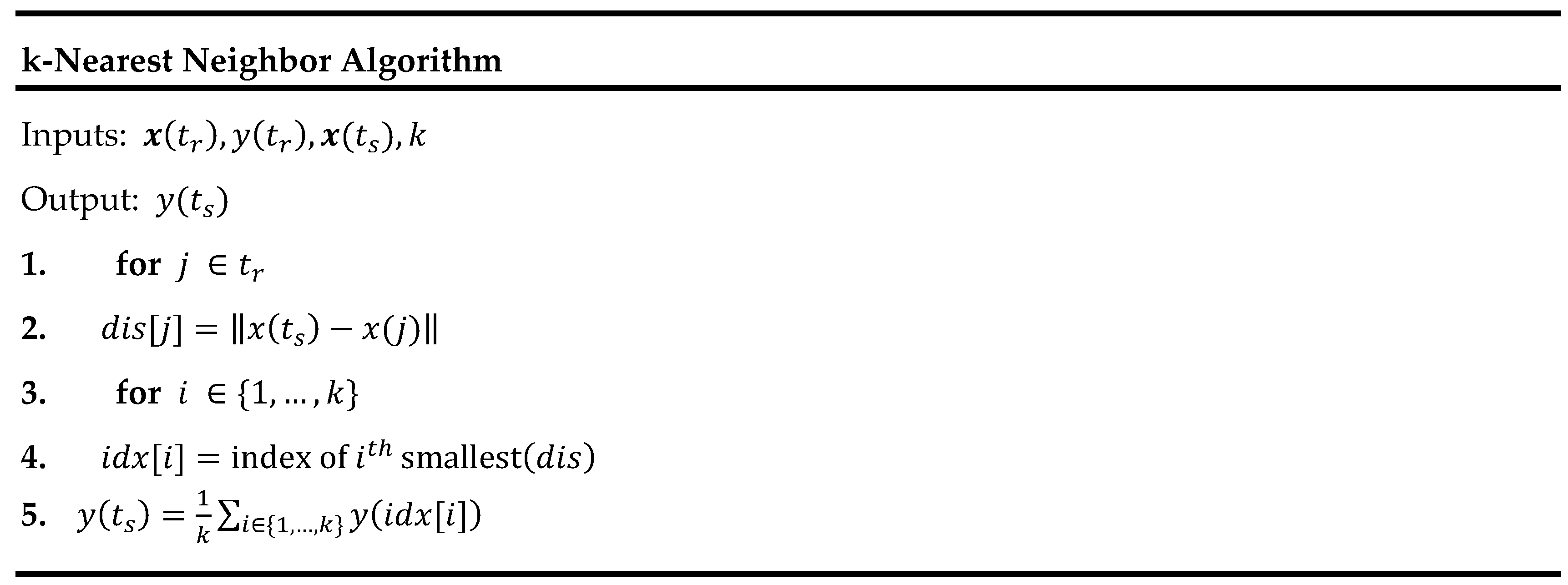
3.1. K-Nearest Neighbor (kNN)

K-Nearest Neighbor is a well-recognized algorithm in the machine learning community [25]. Based on the kNN algorithm, each sample (training, test or validation) is composed of input and output pairs. In this application, the output is one-step ahead solar power generation, y ( t ) = p ( t ) , and the input is the concatenation of the generation records for up to D prior data points, x ( t ) =   { p ( t 1 ) ,   p ( t 2 ) , ,   p ( t D ) } as it is shown in Figure 1b. D is the depth of input which will be determined through cross validation. This concatenation repeats for all of the dataset. That is, if there are N points in the dataset, there will be N D + 1 of these input-output pairs (Figure 1a). Note that it is possible to use only a subset of depths from 1 to D , i.e., D might be pointing to the last 24 h, but algorithm might end up picking the last and first hour of the previous 24-h window, discarding the 22 h in between. In this case, x ( t ) in Figure 1b will have a length of 120 (two sets of 60 min power values). Now, in order to find an estimate for y ( t s ) where t s S t s is an instance of test set indices, first, the dissimilarity between x ( t s ) and all other x ( t r ) , where t r S t r , is computed. Once the k closest x ( t r ) to   x ( t s ) are identified, y ( t s ) would be equal to the average of their matching y ( t r ) . Closeness could be defined as the negative of any dissimilarity measure.
The Euclidean distance is used as a dissimilarity measure in this paper. Figure 2 illustrates the algorithm. The selection procedure for the parameter k is explained in parameter selection (Section 4.2).

3.2. Support Vector Regression (SVR)

The notion behind SVR is to extend the Support Vector Machines (SVMs) concept to regression [26]. In SVM, there is no need to use all training data to form the decision boundaries, rather it turns out a few samples, namely Support Vectors, are enough to predict the class labels. One of the variants of Support Vector Regression algorithm is the ε -SV regression algorithm. In our problem, the forecasting of p ^ ( t ) via ε -SV can be formulated as follows [27]:
  p ^ ( t ) = f ( x ( t ) ) = i = 1 N t r ( α i α i ) G ( x ( i ) , x ( t ) ) + b  
where α i , α i are Lagrange multipliers, x ( i )   is the input vector (as shown in Figure 1b), b R and G ( x i , x j ) is a kernel function. Examples of popular kernels are polynomial, G ( x i , x j ) = ( < x i , x j > +   c ) p , hyperbolic tangent, G ( x i , x j ) = tanh ( a < x i , x j > +   c ) (for some positive a ), and Gaussian radial basis function, G ( x i , x j ) = exp ( γ x i x j 2 ) for γ > 0 .
In this paper, function ‘svm’ in the package ‘e1071’ of the R programming language is used for prediction.

3.3. Random Forest (RF)

The Random Forest algorithm is a randomized aggregated ensemble of decision trees [28]. A decision tree, as the name suggests, is composed of decision nodes to accomplish a set of hierarchical rules and to predict the output value for an unseen input. However, decision trees model data with high variance (i.e., overfitting models) which, simply put, makes them ineffective in generalizing the learned rules. RF is one way to address this shortcoming by training not one tree but a collection of trees (hence forest) and adding randomness at different levels such as random sampling of the training dataset for each tree (hence randomness) [29]. RF has proved to be strong in classification and regression problems [30]. In this paper, function ‘randomForest’ in the package ‘randomForest’ of the R programming language is utilized.

3.4. Auto Regressive Integrated Moving Average (ARIMA)

In ARIMA approach which also is known as Box-Jenkins model, the predicted value of the future variables is modeled as a linear combination of the past values and noise terms [23]. The Auto Regressive (AR) portion models the contribution of the past values of the variable, while the Moving Average (MA) portion models the contribution of noise terms. The Integrated (I) part models the number of differences needed in order to transform the time series to a stationary time series [31]. The ARIMA model is often specified by ARIMA( p , d , q ); p ,   d and q are the order of the AR, I, and MA terms, respectively. Mathematically, ARIMA( p , d , q ) for variable X ( t ) can be written as:
  ( 1 i = 1 p φ i L i ) ( 1 L ) d X ( t ) = ( 1 i = 1 q θ i L i )   ε ( t )  
where L is the lag operator such that L X ( t ) = X ( t 1 ) , ε ( t ) is a representative of the noise (or shock or error) contribution, and φ , θ are the coefficients of the model that need to be determined. For the problem in this paper, the formula can be rewritten as following:
  p ^ ( t ) = ( 1 L ) d ( 1 i = 1 q θ i L i )   ε ( t ) + ( i = 1 p φ i L i ) p ( t )  
Estimation of φ s and θ s is usually done by a fitting method like Maximum Likelihood (ML) estimation once the order of the model (i.e., determining p ,   d and q ) is defined. However, selecting a proper order for the model is usually more challenging, and there is no best method for it. One approach is to use the correlation analysis of the time series and error terms through Autocorrelation Function (ACF) and Partial Autocorrelation Function (PACF). Useful suggestions exist for determining p and q based on ACF and PACF plots but it does not always give the best model [31]. After selecting the model and estimating the parameters using the aforementioned approaches, the fitness of the model to data is examined with criteria such as Akaike Information Criterion (AIC) or Bayesian Information Criterion (BIC) [22]. It is worth mentioning that a better AIC or BIC does not necessarily mean that the model has the least SMAPE or MAE.
In this study, the cross validation was employed to select the best model and determine the ( p , d , q ) tuple that minimizes the MAE. The φ and θ parameters were estimated over the training data for the optimum selected model and are utilized to forecast the test dataset. This paper uses ‘auto.arima’ function of the ‘forecast’ toolbox in the R programming language to select the model order and estimate the parameters [32].

3.5. LinearRegression (LR)

This approach could be interpreted as intersection between ML approaches above (kNN, SVR, RF) and ARIMA: Output would be a linear combination of the historical values (Auto Regressive part from ARIMA) in the same format used for ML algorithm and presented in Figure 1. Specifically, considering Figure 1b, y ( t ) = α . x ( t ) = α 1 p ( t 1 ) + α 2 p ( t 2 ) + + α D p ( t D ) where α , vector of coefficients, is determined by solving least squared error problem on the training set depicted in Figure 1a. We used ‘lm’ function of the ‘stats’ package in the R programming language for implementing this algorithm.

3.6. Persistent

Here, prediction for the next minute’s power equals to the current power, i.e., p ^ ( t + 1 ) = p ( t ) . We have merely included this method as a base line for algorithm comparisons.

4. Simulation Setup

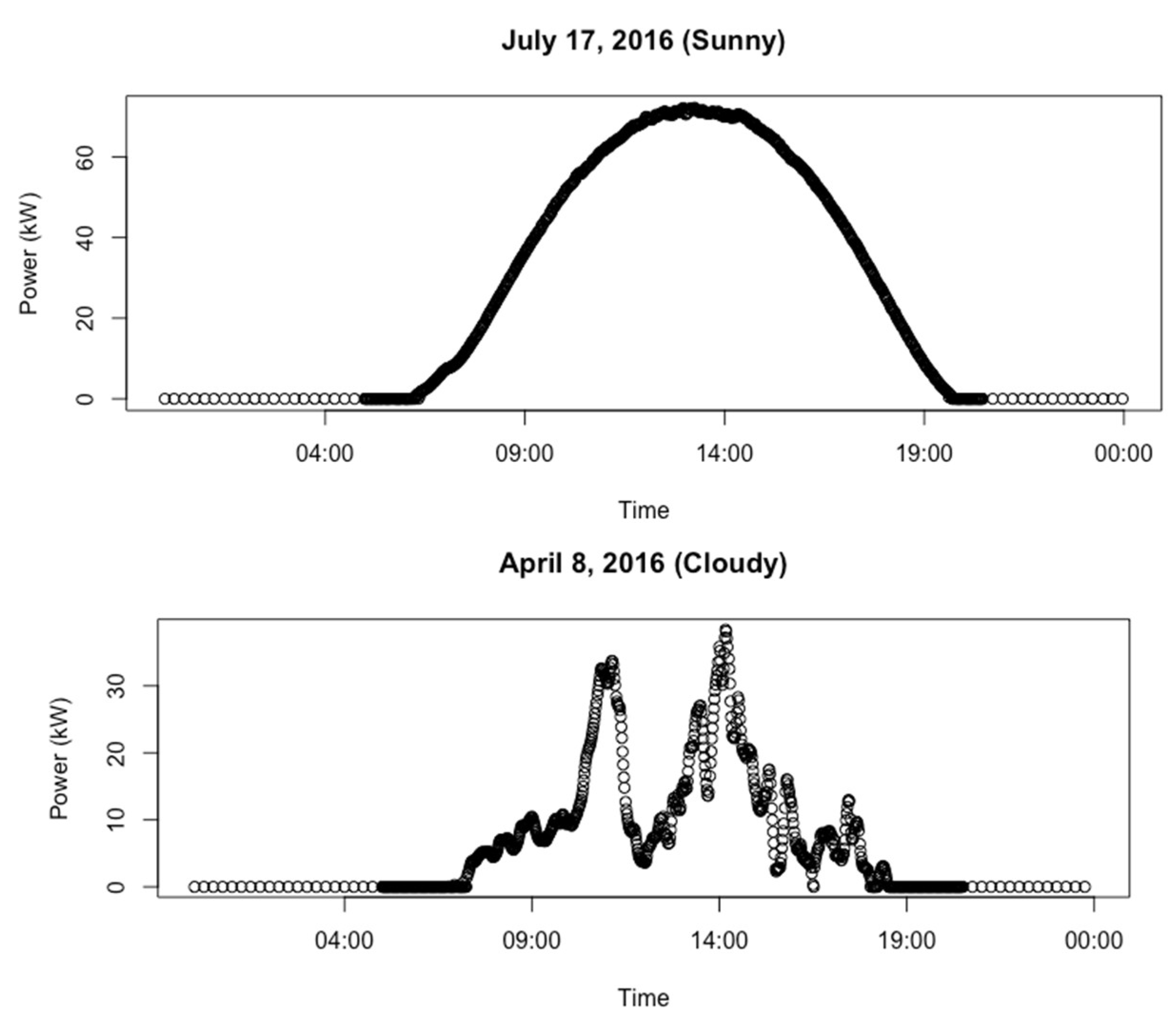
4.1. Data and Preprocessing

The prediction algorithms described in the previous section are applied to the recorded solar power from solar PV panels located on UCR campus. The data used in this paper have 1-min granularity and were recorded from 1 January 2015 to 31 December 2017; however, the measurement was not recorded for this entire time due to communication issues. Missing values and outliers have also been identified and treated. If there is a missing value, the constant imputation is used to substitute the value with zero. On the other hand, if there is more than one measurement in a given minute, the median of them has been used as the power value at that minute. As power generation is a positive value, negative values are considered outliers and are substituted with zero. There was no normalization or feature extracting from the data.
Figure 3 shows sample recorded solar power data for a sunny day (12 February 2015) and a cloudy day (2 December 2014) with 1-min granularity.

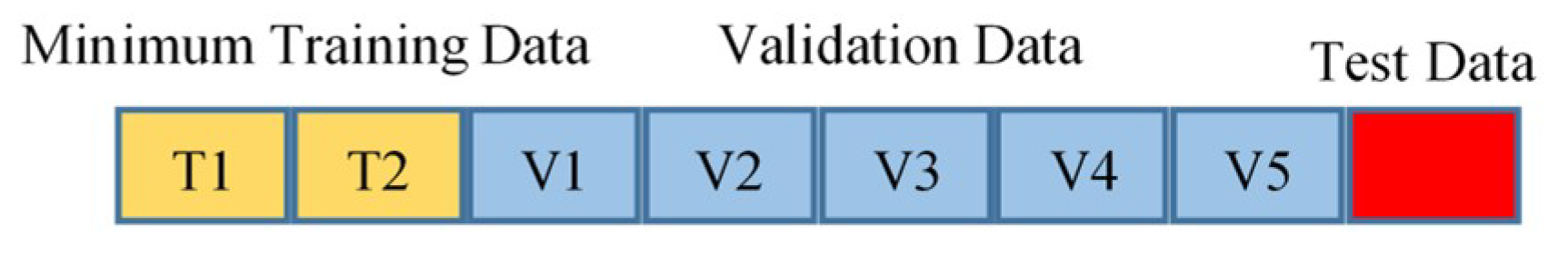
4.2. Parameter Selection

All combinatorial parameters need to be determined via cross validation including Depth ( D ) and number of neighbors ( k ) for kNN; the order of model for ARIMA( p , d , q ); Depth ( D ), the tradeoff coefficient   C , desired   ε , kernel type and its corresponding parameters for the ε -SV; Depth ( D ), minimum number of terminal nodes ( n s ), number of trees ( n t ), and number of variables randomly sampled at each split ( m ) for RF algorithm; and finally Depth ( D ) for LR.
One needs to carefully apply machine learning algorithms to time series forecasting problems, as cross validation might be challenging [33,34]. We have adopted a modified version of the blocked cross-validation introduced in Ref. [35] that incorporates the benefits of both machine learning and time series forecasting literature.
In this version of blocked cross validation, training samples are not shuffled. First, blocks of minimum training data are selected. This is needed to train the first cross validation block. Then, cross validation blocks are selected without changing the order of the time series. The procedure is depicted in Figure 4. with five validation blocks. The algorithm is initially trained on {T1, T2} blocks and is validated on the V1 block; then, it is trained on {T1, T2, V1} blocks and validated on the V2 block, and so on, up until training on {T1, T2, V1, …, V4} and evaluating on V5 block. The advantage of this cross validation method is using the maximum available data compared with the last block validation method and simultaneously preserving the temporal order in time series data.
The depth parameter ( D ) is structured as following: D = ( 1 : d ) , ( d / 2 : d / 2 ) + 24 × 60 ,   ( d / 2 : d / 2 ) + 24 × 60 × 365 and we treat ( d ) as a parameter in cross validation. This translates to d most recent power values, power values of the last 24 h in d neighborhood of the output, as well as power values of the last year in d neighborhood of the output. This structure for depth takes into account both daily and annual periodicities, while limiting the search space in favor of less computation and time. In cross validation, d varies between 2 and 60.
The number of neighbors (k) varied between 1 and 10 for kNN. In addition, in the “auto.arima” function, maximum of p and q was set to 5 and 8 respectively. Parameter d was picked by the auto.arima function based on the Kwiatkowski–Phillips–Schmidt–Shin (KPSS) test [32]. The candidates for our SVR kernel are linear, polynomial, sigmoid, and radial basis kernels. Other than kernels, the selection of parameters for SVR are: ε { 0.01 , 0.1 } and C = { 0.1 ,   1 } , where the bold parameter is the default value in the relevant R package. More details of the parameter determination in an SVR model can be found in Ref. [36]. Regarding RF, the parameters are the number of trees, n t { 200 , 500 } , number of variables at each node to consider for splitting, m { 1 6 , 1 3 , 2 3 } × D , and minimum size of terminal nodes, n s { 5 , 10 } . Many other parameters exist for SVR and RF where their default values in the relevant R package have been selected [32].

5. Results and Analysis
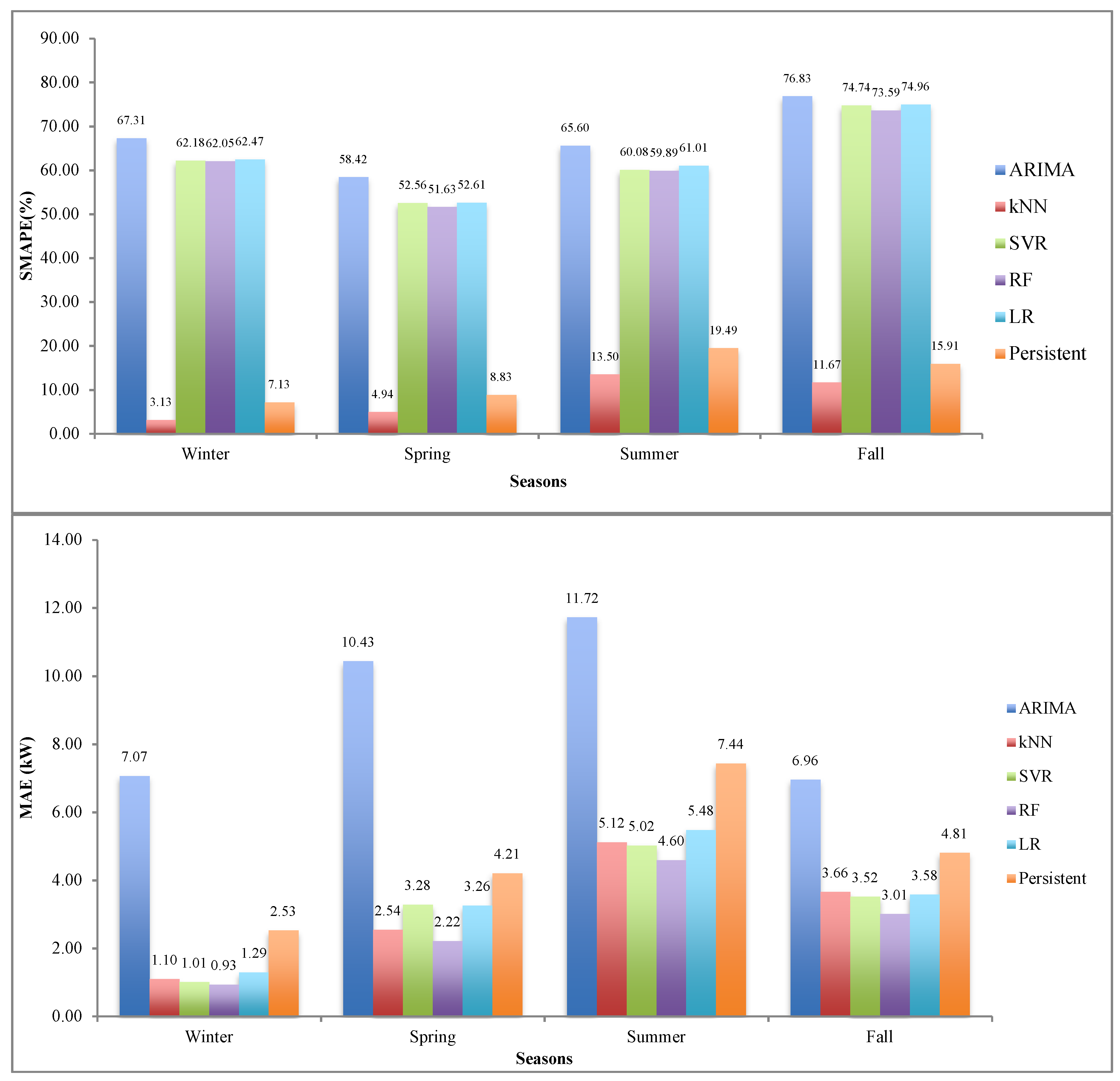
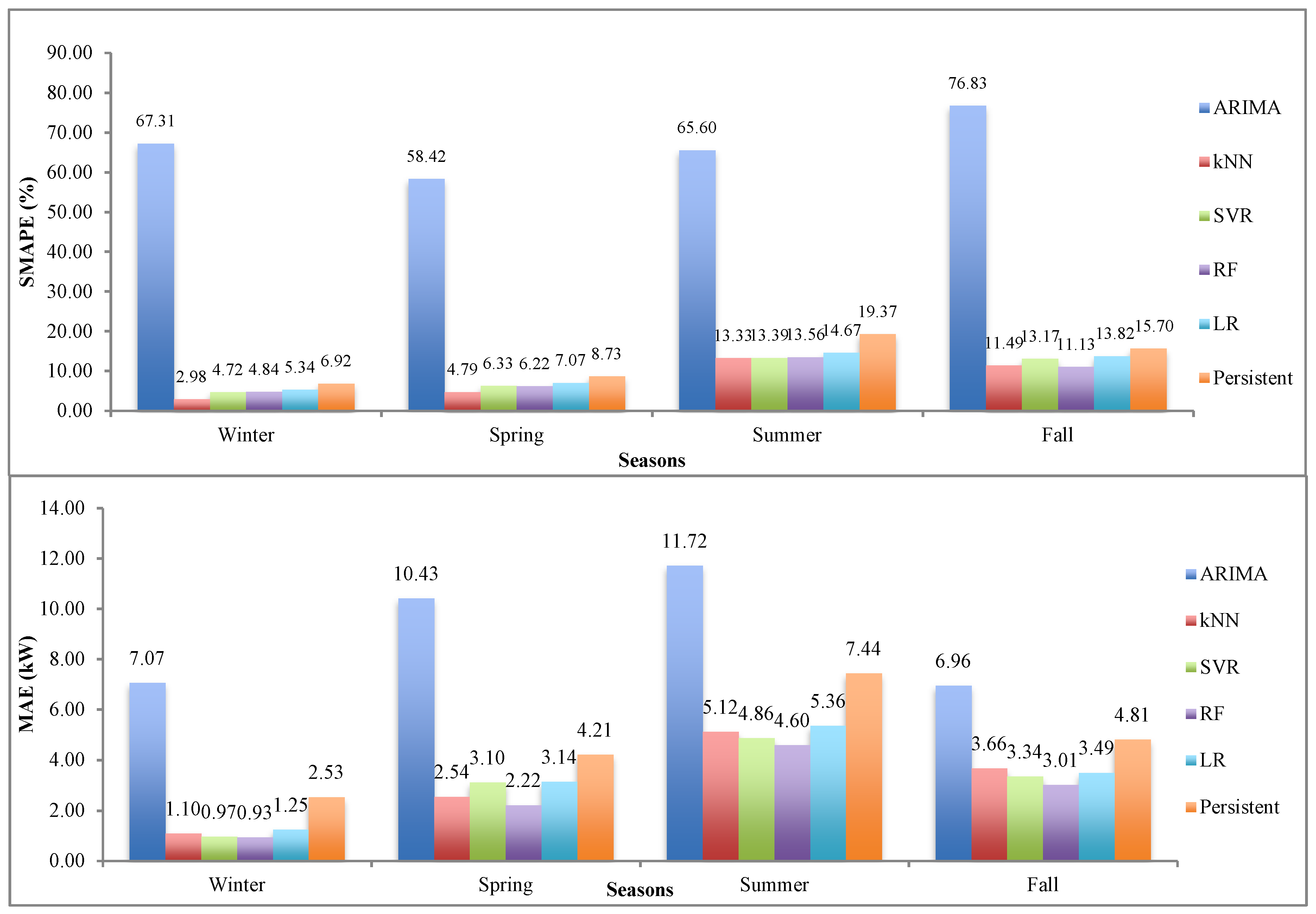
5.1. Results

We picked 4 weeks in four seasons as test samples. For each of the test samples, we trained the models with about 1.5 years of data ending immediately before that week. For instance, when predicting the week of 8 February to 15 February 2017, training data was from August 2015 all the way to 6 February 2017. We used five blocks in the cross-validation procedure. Table 1, shows the selected days in each season:
Figure 5 shows the SMAPE and MAE for each algorithm in four seasons while Table 2 shows the optimum selected parameter for each algorithm.
According to Figure 5, kNN has the best overall performance. Its relative error, SMAPE, is significantly better than the other algorithms and its absolute error, MAE, is comparable with RF and SVR’s MAE. Although all three kNN, SVR, and RF algorithms have comparable absolute errors (MAE), their relative error (SMAPE) is very different. This phenomenon has been discussed in depth in the Analysis subsection of this paper. ARIMA fails to accurately predict according to both criteria, which is not unexpected since the model is essentially AR and only relies on the past five observations and does not capture any periodicity. LR, however, uses the same structure for input features as other ML algorithms and, therefore, is forced to use daily and annual periodicity which leads to much better performance than ARIMA which is generated by using auto.arima package in R.
As Table 2 shows, the selected depth for all the algorithms is rather short, i.e., in kNN, SVR, and RF the prediction is made by looking at the last 10 min of observations along with the corresponding 10 min 24 h ago as well as a year ago. Even p in ARIMA (the order of Auto-Regressive model) has been selected as five, which is equivalent to considering the last 5 min of values. Hence, once again, optimum parameter selection emphasizes the importance of local patterns in short-term times series prediction rather than global patterns.
As mentioned earlier, the prediction process should not take more than a few seconds, so that the entire control process can finish in 1 min. Table 3 shows the execution time for each algorithm once they are provided with the query. Clearly, all algorithms are able to respond to the query in less than a fraction of a second, which is well below a few seconds limit. It is noteworthy to mention the higher response time for kNN, as it is considered a lazy learning (or Instance-based) algorithm, such that no learning has been performed unless a query is received. Therefore, it is not surprising if it takes longer, as the other algorithms are trained offline but kNN is not. Note that for each query, kNN searches the whole training data set and as data grows, the response time will increase too. The 103 milli-seconds is for searching in about 1.5 years of data.
Furthermore, the training time for other algorithms (and the parameter selection time for kNN), which could take a couple of hours, is not factored in, in Figure 6. The training/parameter selection can be done offline and periodically (every week in this paper) so it should not interfere with the querying part. Depending on the computation cost, running the training/parameter selection more often will generate the same or better accuracies. The training time for each algorithm is reported in Table 4, which is the amount of time needed for training after best parameters are determined according to the approach described in Section 4.2.
Unsurprisingly, the training time increases with the increase in the complexity of the model, hence kNN gets the lowest training time and RF gets the highest. Please note that the reported timings might change depending on the computation hardware and should be used as relative guide between algorithms.
In this paper, the simulations have been performed with RStudio version 1.1.423 on an Intel Core i-7 CPU at 2.50 GHz with 16 GB RAM. RStudio is running under R version 3.4.3.

5.2. Analysis

The results reveal interesting characteristics of each of the applied algorithms. The low SMAPE of the kNN algorithm can be justified as follows: According to (2), SMAPE is 100% when either the predicted or actual value (and not both of them) is equal to zero. Considering that in kNN the prediction is always an instance of the past data and the fact that there are lots of zeros in a 24-h period (especially at night, refer to Figure 3), there will be lots of instances that actual power and the prediction are zero, hence yielding a SMAPE equal to zero. However, in other algorithms, as more arithmetic is involved, chances are that their prediction for night time is a very small number but not exactly zero, which makes the SMAPE of that time equal to 100%. However, this type of error in prediction has a lot less effect on MAE measure; therefore, MAE for other algorithms is much better compared to MAE for kNN.
In order to address the discrepancy in SMAPE, the modified version of SVM, RF, and ARIMA algorithms are proposed where the small predicted values in the algorithms are set to zero. In this application, since the peak of the values is in the range of 75 kW and the first value after night hours is in the order of 300 W, the threshold is set to 250 W. With this modification, the results are depicted in Figure 6.
Thresholding the predicted values almost does not change the MAE, but changes the SMAPE for SVR and RF drastically. In case of ARIMA, as the minimum of predicted values is around 5 kW, thresholding with 250 W would not change the predicted values and error measurements.
When considering the thresholding, RF generates the best results with respect to both MAE and SMAPE measurements; however, kNN is following very closely in both measures. In order to have a concrete measure of statistical significance between these algorithms, we have applied Diebold-Mariano test [37] to prediction residuals. Table 5 shows the results of Diebold-Mariano test on pairs of the algorithms.
The test has been performed on concatenating all the residuals from four seasons per each algorithm. Thus, for each algorithm, the residuals of the 4 weeks mentioned in Table 1 (1 week of each season) form the residual vector which contains 40,320 ( 4 × 7 × 24 × 60 ) samples. With choice of α = 0.01 , any value less than 0.01 in entry (alg1, alg2) of Table 4 means that the forecasts of alg1 are statistically, significantly more accurate than those of alg2. For instance, persistent is statistically significantly more accurate than the ARIMA model or RF is statistically significantly more accurate than all other algorithms. Also, all applied algorithms except ARIMA are statistically significantly more accurate than the persistent model.
Considering that parameter selection for kNN will be relatively faster (according to Table 2, SVR and RF both have four parameters to select while kNN only has two), it could be a suitable substitute for RF, when the simplicity of the algorithm is required.

6. Conclusions

In this paper, four well-known algorithms including ARIMA, KNN, SVR, and RF, for fast and super-short-term prediction of solar power generation have been investigated and compared. The goal is to predict the solar-generated power one-step ahead to be used in dynamic control of solar + energy storage systems for solar intermittency compensation. Due to fast response criterion of prediction, the prediction algorithms only rely on historical values of the time series and compare local temporal patterns to make the prediction. To this end, the obtained data from UCR PV panels is cleansed and treated with respect to missing values and outliers. A modified version of the blocked cross-validation, which maximizes the use of available data while preserving the temporal order in time series data, is proposed to design the prediction parameters of each algorithm. In the parameter selection phase, based on the obtained results for all investigated algorithms, the optimum depth of data required for prediction (the one that results in a lower MAE) is obtained which is the last 10 min along with the corresponding 10 min from 24 h ago as well as a year ago. The selection of these short intervals around current moment, daily, and annual periodicities points out the importance of local patterns rather than global patterns in super-short-term time series prediction.
The results of solar prediction using the studied algorithms imply that the performance of each algorithm under different error definition might be different. For example, kNN is the best algorithm when considering SMAPE while RF is the best when it comes to MAE criterion. Therefore, it is important for a system designer to pick an error measurement that models their concerns/costs of the problem properly. In this application, the comparison results show that the machine learning-based algorithms (SVR, RF, and kNN) outperform the traditional ARIMA and trivial persistent algorithms considerably according to MAE and SMAPE criteria. Among the investigated machine learning-based algorithms, RF and kNN outperformed the SVR algorithm, while kNN needs less parameters to be tuned and hence will result in a simpler system.

Author Contributions

Conceptualization, M.M. and H.N.; Methodology, M.M.; Software, M.M.; Validation, M.M, H.N. and H.R.P.; Formal Analysis, M.M.; Investigation, H.N.; Data Curation, R.G.; Writing—Original Draft Preparation, M.M.; Writing—Review & Editing, H.N.; Supervision, R.G. and H.R.P.; Project Administration, P.C.; Funding Acquisition, R.G.

Funding

This research was funded by part from the California Energy Commission (CEC), entitled “Demonstration of PEV Smart Charging and Storage Supporting Grid Operational Needs” grant number EPC-14-056.

Conflicts of Interest

The authors declare no conflict of interest. The funders had no role in the design of the study; in the collection, analyses, or interpretation of data; in the writing of the manuscript, and in the decision to publish the results.

Abbreviations

ACFAutocorrelation Function
AICAkaike Information Criterion
ARAuto Regressive
ARIMAAutoregressive Integrated Moving Average
BICBayesian Information Criterion
GHIGlobal Horizontal Irradiation
IIntegrated
kNN k-Nearest Neighbors
KPSSKwiatkowski–Phillips–Schmidt–Shin
LOCFLast Observation Carried Forward
MAMoving Average
MAEMean Absolute Error
MLMaximum Likelihood
PACFPartial Autocorrelation Function
PVPhotovoltaic
RFRandom Forest
SMAPESymmetric Mean Absolute Percentage Error
SMERCSmart Grid Energy Research left
SVMSupport Vector Machine
SVRSupport Vector Regression
UCR University of California, Riverside

References

  1. Nazaripouya, H.; Chu, C.; Pota, H.R.; Gadh, R. Battery Energy Storage System Control for Intermittency Smoothing Using an Optimized Two-Stage Filter. IEEE Trans. Sustain. Energy 2018, 9, 664–675. [Google Scholar] [CrossRef]
  2. Nazaripouya, H.; Wang, Y.; Chu, P.; Pota, H.R.; Gadh, R. Optimal Sizing and Placement of Battery Energy Storage in Distribution System Based on Solar Size for Voltage Regulation. In Proceedings of the 2015 IEEE PES General Meeting, Denver, CO, USA, 26–30 July 2015. [Google Scholar]
  3. Semero, Y.K.; Zhang, J.; Zheng, D. PV power forecasting using an integrated GA-PSO-ANFIS approach and Gaussian process regression based feature selection strategy. CSEE J. Power Energy Syst. 2018, 4, 210–218. [Google Scholar] [CrossRef]
  4. Tang, N.; Mao, S.; Wang, Y.; Nelms, R.M. Solar Power Generation Forecasting With a LASSO-Based Approach. IEEE Internet Things J. 2018, 5, 1090–1099. [Google Scholar] [CrossRef]
  5. Gigoni, L.; Betti, A.; Crisostomi, E.; Franco, A.; Tucci, M.; Bizzarri, F.; Mucci, D. Day-Ahead Hourly Forecasting of Power Generation From Photovoltaic Plants. IEEE Trans. Sustain. Energy 2018, 9, 831–842. [Google Scholar] [CrossRef]
  6. Verbois, H.; Huva, R.; Rusydi, A.; Walsh, W. Solar irradiance forecasting in the tropics using numerical weather prediction and statistical learning. Sol. Energy 2018, 162, 265–277. [Google Scholar] [CrossRef]
  7. Lauret, P.; David, M.; Pedro, H.T.C. Probabilistic solar forecasting using quantile regression models. Energies 2017, 10, 1591. [Google Scholar] [CrossRef]
  8. Alfadda, A.; Adhikari, R.; Kuzlu, M.; Rahman, S. Hour-ahead solar PV power forecasting using SVR based approach. In Proceedings of the 2017 IEEE Power & Energy Society Innovative Smart Grid Technologies Conference (ISGT), Washington, DC, USA, 23–26 April 2017. [Google Scholar]
  9. Inage, S. Development of an advection model for solar forecasting based on ground data first report: Development and verification of a fundamental model. Sol. Energy 2017, 153, 414–434. [Google Scholar] [CrossRef]
  10. Hong, T.; Pinson, P.; Fan, S.; Zareipour, H.; Troccoli, A.; Hyndman, R.J. Probabilistic energy forecasting: Global Energy Forecasting Competition 2014 and beyond. Int. J. Forecast. 2016, 32, 896–913. [Google Scholar] [CrossRef] [Green Version]
  11. Ferlito, S.; Adinolfi, G.; Graditi, G. Comparative analysis of data-driven methods online and offline trained to the forecasting of grid-connected photovoltaic plant production. Appl. Energy 2017, 205, 116–129. [Google Scholar] [CrossRef]
  12. Graditi, G.; Ferlito, S.; Adinolfi, G.; Tina, G.M.; Ventura, C. Energy yield estimation of thin-film photovoltaic plants by using physical approach and artificial neural networks. Sol. Energy 2016, 130, 232–243. [Google Scholar] [CrossRef]
  13. Huang, R.; Huang, T.; Gadh, R.; Li, N. Solar generation prediction using the ARMA model in a laboratory-level micro-grid. In Proceedings of the 2012 IEEE Third International Conference on Smart Grid Communications (SmartGridComm), Tainan, Taiwan, 5–8 November 2012. [Google Scholar]
  14. Asrari, A.; Wu, T.X.; Ramos, B. A Hybrid Algorithm for Short-Term Solar Power Prediction—Sunshine State Case Study. IEEE Trans. Sustain. Energy 2017, 8, 582–591. [Google Scholar] [CrossRef]
  15. Boualit, S.B.; Mellit, A. SARIMA-SVM hybrid model for the prediction of daily global solar radiation time series. In Proceedings of the 2016 International Renewable and Sustainable Energy Conference (IRSEC), Marrakech, Morocco, 14–17 November 2016. [Google Scholar]
  16. Voyant, C.; Motte, F.; Notton, G.; Fouilloy, A.; Nivet, M.L.; Duchaud, J.L. Prediction intervals for global solar irradiation forecasting using regression trees methods. Renew. Energy 2018, 126, 332–340. [Google Scholar] [CrossRef] [Green Version]
  17. Wang, S.-Y.; Qiu, J.; Li, F.-F. Hybrid Decomposition-Reconfiguration Models for Long-Term Solar Radiation Prediction Only Using Historical Radiation Records. Energies 2018, 11, 1376. [Google Scholar] [CrossRef]
  18. Jiang, Y.; Long, H.; Zhang, Z.; Song, Z. Day-Ahead Prediction of Bihourly Solar Radiance with a Markov Switch Approach. IEEE Trans. Sustain. Energy 2017, 8, 1536–1547. [Google Scholar] [CrossRef]
  19. Grantham, A.; Gel, Y.R.; Boland, J. Nonparametric short-term probabilistic forecasting for solar radiation. Sol. Energy 2016, 133, 465–475. [Google Scholar] [CrossRef]
  20. Nazaripouya, H.; Wang, B.; Wang, Y.; Chu, P.; Pota, H.R.; Gadh, R. Univariate time series prediction of solar power using a hybrid wavelet-ARMA-NARX prediction method. In Proceedings of the 2016 IEEE/PES Transmission and Distribution Conference and Exposition (T&D), Dallas, TX, USA, 2–5 May 2016. [Google Scholar]
  21. Marafiga, E.B.; Farret, F.A.; Peixoto, N.H. Effects of the seasonal sunlight variation on predictions of the solar-aeolic potential for power generation. In Proceedings of the 2015 12th International Conference on the European Energy Market (EEM), Lisbon, Portugal, 19–22 May 2015. [Google Scholar]
  22. Hastie, T.; Tibshirani, R.; Friedman, J. The Elements of Statistical Learning: Data Mining, Inference, and Prediction, 2nd ed.; Springer: Berlin, Germany, 2009. [Google Scholar]
  23. Box, G.E.P.; Jenkins, G.M.; Reinsel, G.C. Time Series Analysis: Forecasting and Control; John Wiley & Sons: Hoboken, NJ, USA, 2013. [Google Scholar]
  24. Majidpour, M.; Qiu, C.; Chu, P.; Gadh, R.; Pota, H.R. Fast Prediction for Sparse Time Series: Demand Forecast of EV Charging Stations for Cell Phone Applications. IEEE Trans. Ind. Inform. 2015, 11, 242–250. [Google Scholar] [CrossRef]
  25. Bishop, C.M. Pattern Recognition and Machine Learning; Springer: New York, NY, USA, 2006. [Google Scholar]
  26. Smola, A.J.; Schölkopf, B. A tutorial on support vector regression. Stat. Comput. 2004, 14, 199–222. [Google Scholar] [CrossRef] [Green Version]
  27. Majidpour, M.; Qiu, C.; Chu, P.; Pota, H.R.; Gadh, R. Forecasting the EV charging load based on customer profile or station measurement. Appl. Energy 2016, 163, 134–141. [Google Scholar] [CrossRef]
  28. Breiman, L. Random forests. Mach. Learn. 2001, 45, 5–32. [Google Scholar] [CrossRef]
  29. Breiman, L. Some properties of splitting criteria. Mach. Learn. 1996, 24, 41–47. [Google Scholar] [CrossRef]
  30. Caruana, R.; Niculescu-Mizil, A. An empirical comparison of supervised learning algorithms. In Proceedings of the 23rd International conFerence on Machine Learning, Pittsburgh, PA, USA, 25–29 June 2006. [Google Scholar]
  31. Weisang, G.; Awazu, Y. Vagaries of the Euro: An Introduction to ARIMA Modeling. Case Stud. Bus. Ind. Gov. Stat. 2008, 2, 45–55. [Google Scholar]
  32. Hyndman, R.J.; Khandakar, Y. Automatic time series forecasting: The forecast package for R. J. Stat. Softw. 2008, 27. [Google Scholar] [CrossRef]
  33. Bergmeir, C.; Benítez, J.M. On the use of cross-validation for time series predictor evaluation. Inf. Sci. 2012, 191, 192–213. [Google Scholar] [CrossRef]
  34. Opsomer, J.; Wang, Y.; Yang, Y. Nonparametric regression with correlated errors. Stat. Sci. 2001, 16, 134–153. [Google Scholar]
  35. Majidpour, M.; Qiu, C.; Chu, P.; Gadh, R.; Pota, H.R. Modified pattern sequence-based forecasting for electric vehicle charging stations. In Proceedings of the 2014 IEEE International Conference on Smart Grid Communications (SmartGridComm), Venice, Italy, 3–6 November 2014. [Google Scholar]
  36. Hong, W. Application of seasonal SVR with chaotic immune algorithm in traffic flow forecasting. Neural Comput. Appl. 2012, 21, 583–593. [Google Scholar] [CrossRef]
  37. Diebold, F.; Mariano, R. Comparing Predictive Accuracy. J. Bus. Econ. Stat. 1995, 13, 253–263. [Google Scholar] [Green Version]
Figure 1. (a) input-output pairs and division of data into training and test sets, (b) labeling inputs as x and outputs as y .
Forecasting 01 00008 g001
Figure 2. k-Nearest Neighbor Algorithm.
Forecasting 01 00008 g002
Figure 3. Sample recorded solar power data for a sunny day (17 July 2016) and a cloudy day (8 April 2016).
Forecasting 01 00008 g003
Figure 4. Modified blocked cross validation. Training data is divided to minimum training data {T1, T2} and validation data {V1, …, V5}.
Forecasting 01 00008 g004
Figure 5. Symmetric Mean Absolute Percentage Error (SMAPE) and Mean Absolute Error (MAE) averaged on test days for each algorithm for each season.
Forecasting 01 00008 g005
Figure 6. Symmetric Mean Absolute Percentage Error (SMAPE) and Mean Absolute Error (MAE) averaged on test days for each algorithm including the thresholding effect: The output values of ARIMA, SVR, and RF algorithms that are less than 250 W are rounded to zero.
Forecasting 01 00008 g006
Table 1. Test samples from each season.
SeasonStartEnd
Winter8 February 201714 February 2017
Spring8 May 201714 May 2017
Summer7 August 201613 August 2016
Fall15 November 201621 November 2016
Table 2. Optimum selected parameter for each algorithm.
ParameterARIMAkNNSVRRFLR
Parameter ( d ) in Depth ( D )--10101010
Neighbor ( k )--1------
Order (p,d,q)(5,0,0)--------
Kernel --Polynomial----
ε ----0.01----
Cost ( C )----1----
Number of trees ( n t )------200--
Splitting leaves at each node ( m )------ 1 2 D   = 5--
Minimum of terminal nodes ( n s )------5--
Table 3. The average time (in milli-seconds) for each algorithm to make a 1-min ahead prediction.
AlgorithmARIMAkNNSVRRFLR
Prediction Time (ms)41033.12642.56
Table 4. Training Time for Each Algorithm with Optimal Parameters.
AlgorithmARIMAkNNSVRRFLR
Training time with optimal parameters (s)25.220.0323.84542.330.13
Table 5. Diebold-Mariano test results.
AlgorithmARIMAkNNSVRRFPersistentLR
ARIMA--11111
kNN0.0000--0.006110.00000.0000
SVR0.00000.9938--10.00000.0000
RF0.00000.00000.0000--0.00000.0000
Persistent0.000011 1--1
LR0.00001110.0000--

