Tuning the Bivariate Meta-Gaussian Distribution Conditionally in Quantifying Precipitation Prediction Uncertainty

1
National Weather Service, Office of Water Prediction, 1325 East-West Highway, Silver Spring, MD 20910, USA
2
Lynker, 202 Church Street, SE/Suite 536, Leesburg, VA 20175, USA
Forecasting 2020, 2(1), 1-19; https://0-doi-org.brum.beds.ac.uk/10.3390/forecast2010001
Submission received: 25 November 2019
/
Revised: 2 January 2020
/
Accepted: 10 January 2020
/
Published: 15 January 2020
(This article belongs to the Special Issue Advances in Hydrological Forecasting)
Abstract
:One of the ways to quantify uncertainty of deterministic forecasts is to construct a joint distribution between the forecast variable and the observed variable; then, the uncertainty of the forecast can be represented by the conditional distribution of the observed given the forecast. The joint distribution of two continuous hydrometeorological variables can often be modeled by the bivariate meta-Gaussian distribution (BMGD). The BMGD can be obtained by transforming each of the two variables to a standard normal variable and the dependence between the transformed variables is provided by the Pearson correlation coefficient of these two variables. The BMGD modeling is exact provided that the transformed joint distribution is standard normal. In real-world applications, however, this normality assumption is hardly fulfilled. This is often the case for the modeling problem we consider in this paper: establish the joint distribution of a forecast variable and its corresponding observed variable for precipitation amounts accumulated over a duration of 24 h. In this case, the BMGD can only serve as an approximate model and the dependence parameter can be estimated in a variety of ways. In this paper, the effect of tuning this parameter is studied. Numerical simulations conducted suggest that, while the parameter tuning results in limited improvements in goodness-of-fit (GOF) for the BMGD as a bivariate distribution model, better results may be achieved by tuning the parameter for the one-dimensional conditional distribution of the observed given the forecast greater than a certain large value.
1. Introduction
The bivariate meta-Gaussian distribution (BMGD), introduced by Kelly and Krzysztofowicz [1], is well suited for modeling the joint distribution of two hydrometeorological variables [2,3,4,5,6]. The BMGD offers a flexible model because each of its marginal variables can be specified independently with any suitable univariate probability distribution. This is a very attractive feature as individual variables in a model may be better fitted by probability distributions from various families. For example, (1) the Weibull and gamma distributions are good candidates for fitting accumulated precipitation amounts [5,7,8,9,10], and (2) the lognormal distribution can provide a good fit for mean area average rain rate [11] and for streamflow data in wet seasons [12].
The BMGD was employed in several recent studies in the area of post-processing ensemble weather forecasts. As a way of quantifying predictive uncertainty of precipitation forecasts, Wu et al. [5] explored a mixed-type BMGD in producing precipitation ensemble forecasts. Schaake et al. [4] applied the BMGD in producing precipitation and temperature ensemble forecasts. The BMGD is used in producing precipitation and temperature ensemble forecasts based on a number of forecast products from numerical weather prediction models [13]. Validation results indicate that the BMGD is a suitable model for use in producing reliable precipitation and temperature ensemble forecasts for hydrologic ensemble forecasting [14,15]. The BMGD is extended in [16] to a wider class of probability distributions with given marginals, known as meta-elliptical distributions. This extended model was shown by [17] to be flexible in modeling trivariate hydrologic data.
The BMGD can be formulated in two different ways. Although both lead to the same end result in terms of the form of probability distribution, there is a subtle difference in the assumption for the model’s dependence structure. In the conventional approach, which is characterized by the construction of a bivariate probability density weighting function [2], one transforms each of the variables to a standard normal variable. A key assumption of this formulation is that the transformed variables are jointly normal. In real-world applications, this assumption may not hold. Herr and Krzysztofowicz [8] conducted a study on the normality hypothesis with the use of 24-h precipitation data collected at a number of rain gauge locations in two river basins in the Appalachian Mountains. Their findings are mixed: for one basin, the normality hypothesis was not rejected in most of the cases; for the other basin, the hypothesis was rejected in most of the cases, albeit possibly of little practical concern. To further illustrate this point, Section 4.2 of this paper gives two examples showing that this normality assumption can be invalid for the cases under consideration. In the next section, it is shown that this assumption can be dropped if we formulate the BMGD using the Gaussian copula to yield an approximate model. With this approach, the BMGD becomes more flexible in that the dependence parameter of the distribution is not constrained by the data for modeling the marginal distributions. The theoretical implication of this relaxation is that the model can be tuned by adjusting the dependence parameter.
This work is primarily concerned with tuning the dependence parameter of the BMGD so that the model can fit the data better. The tuning is investigated for the BMGD as a bivariate distribution model (unconditional tuning) and for the one-dimensional conditional distribution of the observed given the forecast greater than a certain large value (conditional tuning). In the context of generating ensemble forecasts from the BMGD model, the adjustment pertains to a major objective of ensemble post-processing: reliability, which refers to statistical consistency between a priori predicted probabilities and a posteriori observed frequencies of the occurrence of an event under consideration [18]. If the data sample is sufficiently large, then a better fit of the model would translate to more reliable ensemble forecasts. The fit of the model may be improved by selecting more suitable marginal distributions as well as tuning the dependence parameter of the model. In this study, the focus is on model tuning in which both unconditional tuning and conditional tuning are explored.
This paper is organized as follows: Section 2 describes the two different approaches for formulating the BMGD. First, a brief description of the conventional approach is given. Then, a formulation with the copula approach is laid out. Methods used in this study for estimating the dependence parameter is also described. Section 3 describes a bivariate distribution model for an observed variable and its corresponding forecast variable for precipitation amounts. The model accounts for precipitation intermittency explicitly. Equations characterizing the intermittency are derived using calculus and elementary probability theory. In this model, the portion of the joint distribution where both variables are positive is separated out so that it can be modeled by the BMGD. Section 4 describes the numerical experiments conducted in this study. It includes a description of the experimental data and simulation processes, and a discussion of some results. Section 5 provides the discussion, and the final section gives the conclusions.
2. Bivariate Meta-Gaussian Distribution
2.1. Formulation
The conventional approach starts with a density weighting function [1,2]. A normality assumption is made with this approach. The following gives a description of how the BMGD can be obtained, without reference to the density weighting function, for easy comparison with the alternative approach. Consider the joint cumulative distribution function (CDF) of two continuous variables X and Y:
Denote the CDF of X and Y by and , respectively. Assume that and are strictly increasing. Let denote the standard normal distribution function and its inverse. The X and Y can be transformed to obtain two standard normal variables Z and W: and . The transformation involved is known as normal quantile transform (NQT). It follows that , where and . Let denote the Pearson product-moment correlation coefficient between Z and W. If we assume that
where is the standard bivariate normal distribution with correlation coefficient , and define
then we have
Equation (3) is termed as meta-Gaussian distribution of X and Y [1], which is an exact model for under the normality assumption of .
This normality assumption, however, may not hold in certain real-world applications. If that is the case, it seems that what one can hope is that is still close to . This leads to the question of whether we can tune the model to make it closer to . In particular, we ask whether an optimal value can be found to replace the -value obtained by transforming X and Y, such that the model is optimal under a given performance criterion. Furthermore, we ask whether is still a CDF with replaced by an arbitrary value in the unit interval. While the first question may be tackled by conducting numerical experiments, the second question can be answered using the copula theory. Indeed, using the Gaussian copula, we can redefine the BMGD with decoupled from X and Y.
The bivariate Gaussian copula has the following form [19]:
where is the bivariate standard normal distribution with correlation parameter in , u and v take values in the unit interval. Writing and , we recognize that the right-hand side of (3) becomes a Gaussian copula. Conversely, given a bivariate Gaussian copula and two CDFs and , Sklar’s theorem [20], entails that
is a joint CDF with marginal distributions and . Here, we use in the equation to emphasize that its value is not necessarily the same as that of , which is obtained from X and Y. Generally, is the CDF of a random vector with X and Y as its marginal variables and a dependence structure that is different than that of . Note that is not equal to even when unless the normality condition given by (2) holds. Here, we denote this random vector by and refer to (6) as the meta-Gaussian distribution induced from X and Y. Clearly, the BMGD is simply the bivariate Gaussian copula expressed in the original variables. While is an BMGD with an arbitrarily specified value in , to obtain an approximate model to , the dependence parameter needs to be estimated using some estimator.
Equation (7) below is used in the simulation study of this work. For , let denote the conditional distribution of Y given . An expression for is given in Appendix A. For a value of p in , the p-probability conditional quantile of Y given is a value of Y such that . From Equation (A2) in Appendix A, we have
This equation is also given in [21], obtained by taking partial derivative of the copula with respect to u, wherein the quantity is referred to as the p-th copula quantile curve of y conditional on x.
2.2. Estimation of the Dependence Parameter
The dependence parameter can be estimated once the marginals are specified. This estimation approach exploits the fundamental idea of separation between the univariate marginals and the dependence structure of the copula theory. Three estimation methods are described here.
2.2.1. Pearson’s Correlation
Apparently, we can let , the Pearson’s correlation coefficient between the two standard normal variables Z and W, defined in the previous section. In theory, if the normality condition holds, this value renders the BMGD modeling exact.
2.2.2. Maximum Likelihood
The method of maximum-likelihood is commonly used in parameter estimation for a statistical model. The maximum likelihood estimator (MLE) is statistically consistent and asymptotically normally distributed [22]. In this work, the method is used to estimate only the dependence parameter (separated from estimating parameters of the marginals), which can be thought as the second stage of the two-stage procedure for estimating copula parameters [23]. An application of this method in the context of multivariate meta-Gaussian distribution models is given by [24].
The MLE for in can be obtained by following the standard procedure. Assume we have a sample of n points: . The likelihood function is
The corresponding log-likelihood function is
Setting the derivative of the log-likelihood function to zero yields the following cubic equation:
where and are related to and , respectively, through NQT described earlier in this section. The MLE is given by the real root of the above equation. Let and . Let , , and . The real root of (8) is the following:
2.2.3. Minimization of the Mallows Distance
The Mallows distance is a similarity measure between two probability distributions. It can be defined in a number of ways at various levels of abstraction. Here, the one in [25] is given. Let P and Q be probability distributions on . Consider joint distributions of the form with X following P and Y following Q. Let F be a joint distribution of X and Y. The Mallows distance between P and Q can be defined by the minimum of the expected difference between X and Y, taken over all joint probability distributions F:
where is usually taken to be the Euclidean or norm and . In this study, we set , in light of the fact that if P and Q are one-dimensional, the Mallows distance is simply the area between the two CDF curves [25]. This particular case is recognized as the area validation metric [26] in the discussion of proper divergence functions for evaluating differences between model output probability distributions and the corresponding empirical distributions of the data. Some important properties of the Mallows distance are given in [25,27].
The Mallows distance is related to another similarity measure known as earth mover’s distance (EMD), introduced by [28] in the context of image retrieval. The Mallows distance is equivalent to the EMD when the EMD is applied to probability distributions. The equivalence, on the one hand, provides theoretical justification for the EMD by the theory of the Mallows distance, as shown by [25]; and, on the other hand, offers efficient algorithms available to the EMD for computing the Mallows distance numerically. Thus, optimal dependence parameter values are obtained by minimizing the EMD.
The EMD is a general and flexible metric for evaluating similarity or distance between two multi-dimensional distributions. The EMD is a cross-bin comparison measure. As such, it is more robust than those bin-by-bin comparison measures (histogram matching techniques such as Minkowski-form distance and histogram intersection). Bin-by-bin comparison measures have two major drawbacks: (1) they account only for similarity between corresponding bins; and (2) they are sensitive to bin size and therefore the selection of a proper bin size is important. By contrast, the EMD also uses information across bins and always yields better results with finer bins. For a detailed discussion of the EMD and its properties, see [28].
3. A Bivariate Distribution Model for Precipitation Amounts
Because of the intermittent nature of precipitation [29], modeling statistical relationships among variables of precipitation amounts can be demanding. For a single variable of precipitation amounts, one can employ a mixed-type distribution model that has a point mass at zero and a continuous probability density function over the positive domain. This modeling approach was adapted in [10] to introduce a mixed-type model for the bivariate case. For this mixed-type bivariate distribution, Herr and Krzysztofowicz [8] formulated equations for conditional distributions given a value of a marginal distribution. A full derivation of the equations using Dirac delta functions were given in [30,31]. In this section, an alternative derivation is given using calculus and elementary probability theory. The derivation also provides a proof for Equation (D1) in [5].
Let X and Y denote accumulated precipitation amounts for a given temporal scale. We note here that and . Denote the joint CDF of X and Y by . Then, can be expressed as:
where
Here, , , and are assumed to be continuous. In this work, is modeled by the BMGD. It is easy to see that the point probability masses sums to 1.
To obtain expressions for the following conditional distribution
we further define:
Then, for , we have
where . If , then , indicating that (13) can not be defined for this case. For , we have
where
with being the density function corresponding to and corresponding to . If , Equation (14) reduces to . If and , then , implying that the case of is void.
A proof for (15) using calculus and elementary probability theory is given in Appendix B. A similar form of this equation can be found in [8], which was derived with the use of Dirac delta functions [31].
4. Numerical Experiments
4.1. Data
The idea of tuning the BMGD model is tested using real-world data. The experimental data sets are collected for drainage basins or sub-areas of drainage basins. For the observed variable, historical values of 6-hly mean areal precipitation (MAP) for the drainage areas are used. For the forecast variable, 6-hly precipitation reforecasts generated from the Global Ensemble Forecast System (GEFS) of the U.S. National Centers for Environmental Prediction (NCEP) are used. A more detailed description of the data is given as follows.
The drainage areas considered in this study are selected from the service areas of the Arkansas–Red Basin (AB-), Colorado Basin (CB-), California–Nevada (CN-), and Middle Atlantic (MA-) River Forecast Centers (RFC) of the US National Weather Service (NWS), which are of different geophysical and climate characteristics [14]. Specifically, four drainage areas are selected as follows: the Chikaskia River at Blackwell in Oklahoma at ABRFC (ID: BLKO2); the middle zone of the Dolores River at Dolores in Colorado at CBRFC (ID: DOLC2LMF); the lower zone of the Eel River at Fort Seward in California at CNRFC (ID: FTSC1LLF); and the West Branch Delaware River at Walton in New York at MARFC (ID: WALN6).
The RFC-provided historical precipitation observations are MAP values accumulated over 6-h time periods. These 6-h MAP values came from rain-gauge only analysis or multisensor analysis [32], recorded in local time. Archives of these historical MAP values are available typically for several decades.
The GEFS version used is based on version 9.0.1 of the NCEP Global Forecast System (GFS), which is a deterministic forecast model. The GEFS uses the GFS model to produce a control member and then perturbs it to generate other ensemble members. This version has a horizontal resolution of T254 (∼55 km) for forecast period of days 1–8 and T190 (∼70 km) for forecast period of days 7.5–16. This GEFS version was used by the Earth System Research Laboratory of the US National Oceanic and Atmospheric Administration to produce GEFS reforecast datasets. The datasets are generated for the period between 1985 and 2010 [33]. Of the various configurations available for the GEFS reforecasts, the one used here has 11 ensemble members, produced daily with a forecast start time at 00 UTC.
Corresponding to a given MAP value, the mean value of the ensemble members (the GEFS reforecast ensemble has 11 members) is used for the forecast variable in the construction of the BMGD model. As a side remark, the practice of employing the ensemble mean in ensemble post-processing has been evaluated in several recent studies, conducted using long reforecast records (see, for example, [14]). The results in [14] indicate that the forecast ensembles generated by the BMGD model typically underestimate the largest observed precipitation amounts, but otherwise are reliable.
To create forecast-observation pairs, the 6-hly MAP values (recorded at hours 0, 6, 12, and 18 in local time) are matched with the GEFS ensemble mean values (issued for hours 0, 6, 12, and 18 in UTC) in such a way that their time differences in UTC are minimum. The GEFS reforecasts are gridded datasets. The reforecasts produced at the grid point that is closest to the centroid of the drainage area is selected. This is a regridding method referred to as the nearest neighbor (NN) method in the literature. More sophisticated regridding methods (e.g., bilinear interpolation) can be found in [34]. Whether another method would outperform the NN method depends on factors including the distance between the centroid and the nearest grid point as well as the geophysical and climate characteristics of the drainage area. Table 1 shows the coordinates of the centroid of the drainage areas and those of the corresponding GEFS grid points. We note that the differences between the centroid coordinates and the corresponding grid point coordinates are in the range of 0.06–0.41 degree for the latitude and 0.06–0.22 degree for the longitude, which are deemed small. Thus, the simple NN method is used instead of a more sophisticated method.
4.2. Simulation
The statistical models and procedures described in the previous sections are coded using the R language to perform numerical simulations. Some R routines used in the simulations are obtained from the following R packages of the Comprehensive R Archive Network:
- Package ‘lmomco’: Providing extensive functions for computation of L-moments in addition to probability weighted moments, and parameter estimation for numerous distributions.
- Package ‘emdist’: Providing tools for computing the Earth Mover’s Distance.
Generally, precipitation amounts exhibit seasonal variations. Additionally, the forecast skill of the GEFS varies during the year. To account for these seasonal variations, seasonal windows of about 90 days are used to subset the historical MAP data and GEFS reforecast data so that simulations are performed for each of the four seasons: spring (Mar., Apr., May), summer (Jun., Jul., Aug.), fall (Sep., Oct., Nov.), and winter (Dec., Jan, Feb). For a given season, this study is focused on the forecast period of the first 24 h with precipitation amounts aggregated over the four 6-h sub-periods.
The three parameter Weibull distribution is used for modeling the two marginal distributions of the BMGD and the density functions involved in computing the in Equation (14). Simulated forecasts are generated from the fitted marginal distribution for the forecast. A common rain gauge detection limit is 0.01 inches. This value is used here as the threshold to distinguish between wet and dry conditions. Any MAP values and GEFS reforecast values less than this threshold are set to zero. The choice of the three parameter Weibull in this study is based on goodness-of-fit (GOF) by visual inspection of the CDF and quantile-quantile plots. It is found that the three parameter gamma distribution yields similar results.
The distance between the modeled and the empirical distributions can also be evaluated by comparing their conditional distributions. This way, a particular portion of the BMGD can be assessed for GOF. For example, assessing GOF for conditional distributions given large forecast amounts is important in forecasting heavy precipitation events for flood forecasting. In this experiment, GOF of the conditional distribution of the observed given the forecast greater than the 75th percentile of the forecasts obtained from ensemble mean values of the retrospective GEFS ensemble forecasts is also studied.
The BMGD is dependent on the value of . This simulation study is aimed to evaluate the GOF, unconditionally and conditionally, between the empirical joint distribution and the modeled BMGD as varies. Optimal values may be found when a certain distance measure between the two distributions is minimum. In this study, two distance measures are used: the EMD and the well-known Kolmogorov–Smirnov statistic (KSS). We note here that the KSS is applied only for conditional distributions treated as one-dimensional. For each value, the number of simulated forecast-observation pairs is set to . For a given drainage area and season, a simulation run is executed as follows:
- Loop through a sequence of values. These values are created in increments of a certain step size.
- For a given value, loop to create simulated forecast-observation pairs.
- Draw a sample point from the forecast distribution.
- If this value is zero, generate an observation sample point from the distribution given in Equation (13). In this equation, the constant a dictates the probabilities of drawing a zero value or a non-zero value from .
- If the simulated forecast value is positive, generate an observation sample point from the distribution given in Equation (14). In this equation, the function dictates the probabilities of drawing a zero value or a non-zero value from .
For each value, a value of a distance measure is computed. This gives us a sequence of distance values. These values fluctuate as a function of . To smooth out the fluctuations, a moving average with five steps is applied. The average is taken over the central value and the four values surrounding it.
4.3. Results
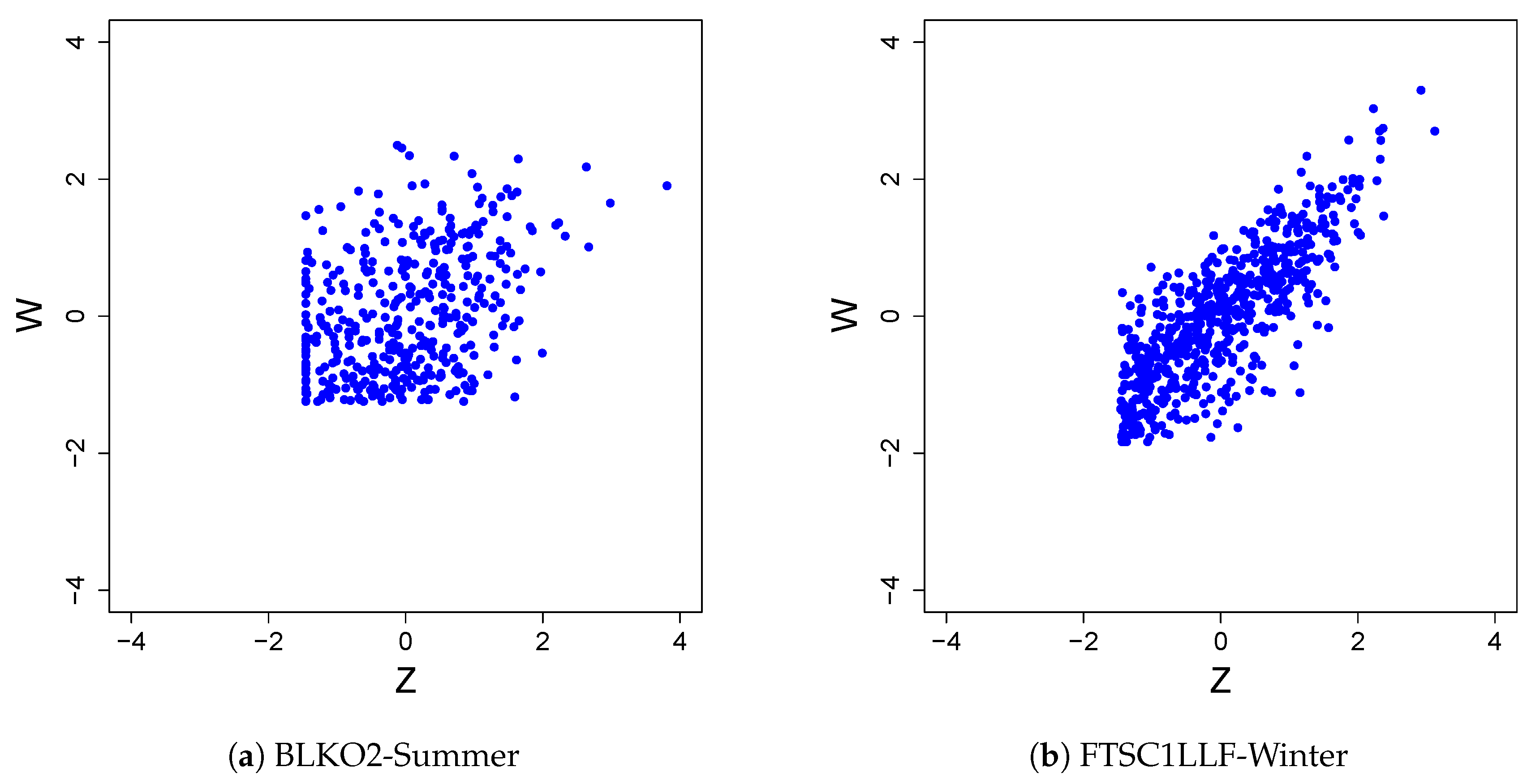
We now illustrate that the normality assumption discussed in Section 2 may fail to hold when dealing with real-world problems. Figure 1 shows the scatter plots of the transformed forecast and observed for drainage areas BLKO2 (a) and FTSC1LLF (b) for summer and winter, respectively. In the plots, the Z-axis represents the forecast and the W-axis the observed. We can see that neither scatter plot has an elliptical shape, a characteristic of the bivariate normal distribution. The straight edges seen in the plots can be attributed to the following: (1) the observed and forecast variables are right-skewed with a relatively large probability mass at the threshold value, which is 0.01 inches (a common rain gauge detection limit); and (2) when the observations are just 0.01 inches, the corresponding forecasts are spread out considerably, and vice versa. The lack of normality may also be caused by the rain gauges’ resolution: for small rainfall values, a high percentage of identical values are yielded. This may affect the transformed variables through NQT.
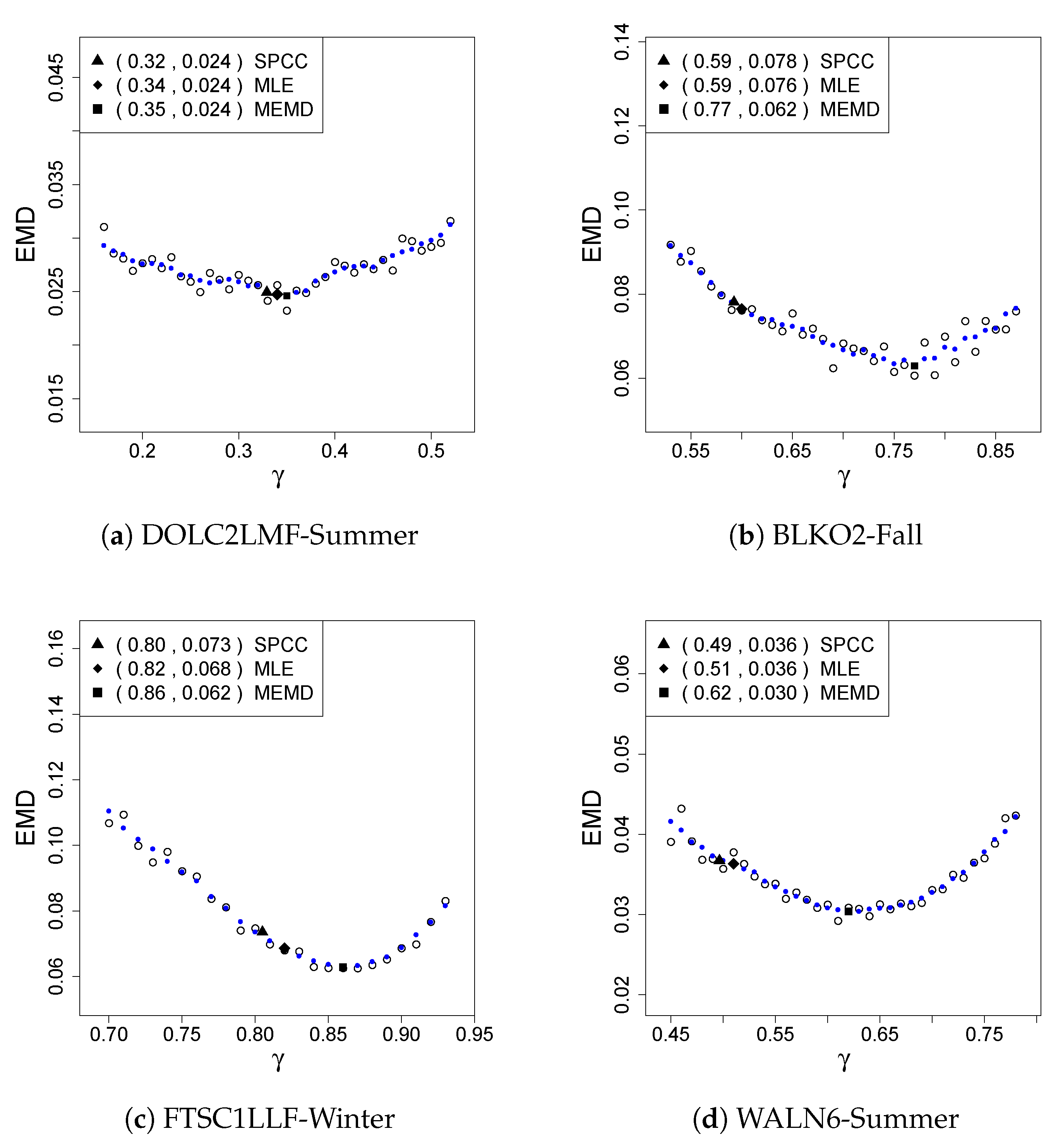
Tuning the dependence parameter unconditionally is examined next. Figure 2 shows EMD values for a sequence of values and contrast them with the EMD values obtained from applying the sample Pearson’s correlation coefficient (SPCC), the maximum likelihood estimate (MLE), and the minimum EMD (MEMD), for the following combinations of drainage areas and seasons: DOLC2LMF-summer (a), BLKO2-Fall (b), FTSC1LLF-Winter (c), and WALN6-Summer (d). In the plots, the circles are EMD values at the corresponding values. The dots give smoothed EMD values. The solid triangle, diamond, and square marks the smoothed EMD values obtained from applying the SPCC, the MLE, and the MEMD, respectively. We can make a few observations from the plots. Firstly, the solid square (MEMD), as the minimum value of the smoothed EMD, is necessarily located below other EMD values in the plots. Secondly, in panel (a), all three methods yield EMD values that are computationally and statistically indistinguishable. Thirdly, the MEMD value is located to the right of the SPCC and MLE values for all four cases. For cases (b), (c), and (d), large percentage reductions in EMD are achieved by the MEMD method in comparison with the other two methods, with the MEMD value much greater than that of the other two methods.
Table 2 presents smoothed EMD values obtained from applying the SPCC, the MLE, and the MEMD for all the drainage areas and seasons considered in this work. We can see that, in the majority of cases, the SPCC and MLE give similar results. For BLKO2, all three methods give close EMD values except for Fall. For DOLC2LMF, the largest difference occurs for Spring where the EMD given by the SPCC is about 17% greater than that given by the MEMD. For FTSC1LLF, relative reduction in EMD ranging from 8% for Fall to about 18% for Winter is achieved by the MEMD. For WALN6, a 20% reduction in EMD occurs for Summer and a 30% reduction for Fall, respectively. For some cases, the results from the three estimation methods are close, statistically indistinguishable. For other cases, significant reductions of 10–20% in EMD are seen by MEMD relative to SPCC or MLE. It is worth noting that, for the case of BLKO2-Summer, despite the obvious lack of normality as indicated by Figure 1a, the MEMD is unable to provide any improvement. The results show that the MEMD performs better only in one-fourth of the cases. Overall, the results indicate that tuning the BMGD unconditionally under the MEMD does not bring much performance improvement over the SPCC and MLE, even though the performance criterion is MEMD itself, which is favorable. This lack of improvement may be explained in the context of conditional tuning. While conditional tuning for the largest quartile (forecast > 75th percentile) is investigated (results will be reported next), conditional tuning for the three smaller quartiles are also examined (results are not presented as the focus of this work is on the largest quartile). There seems to be a tendency that smaller quartiles correspond to smaller conditional tuning values. It stands to reason that a value yielded by the unconditional tuning represents the middle ground of the conditional tuning values. This middle ground value lies close to the SPCC and MLE values in the majority of cases.
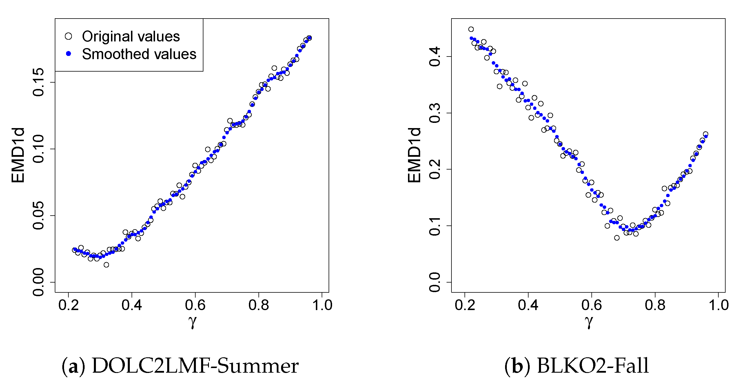
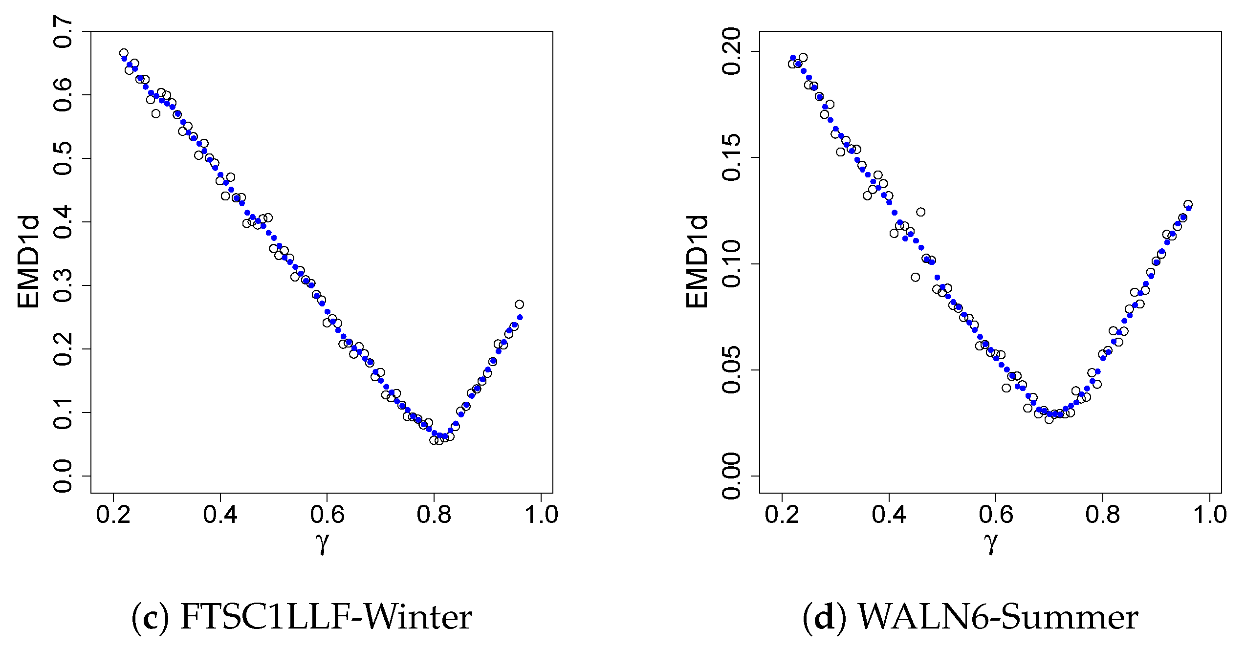
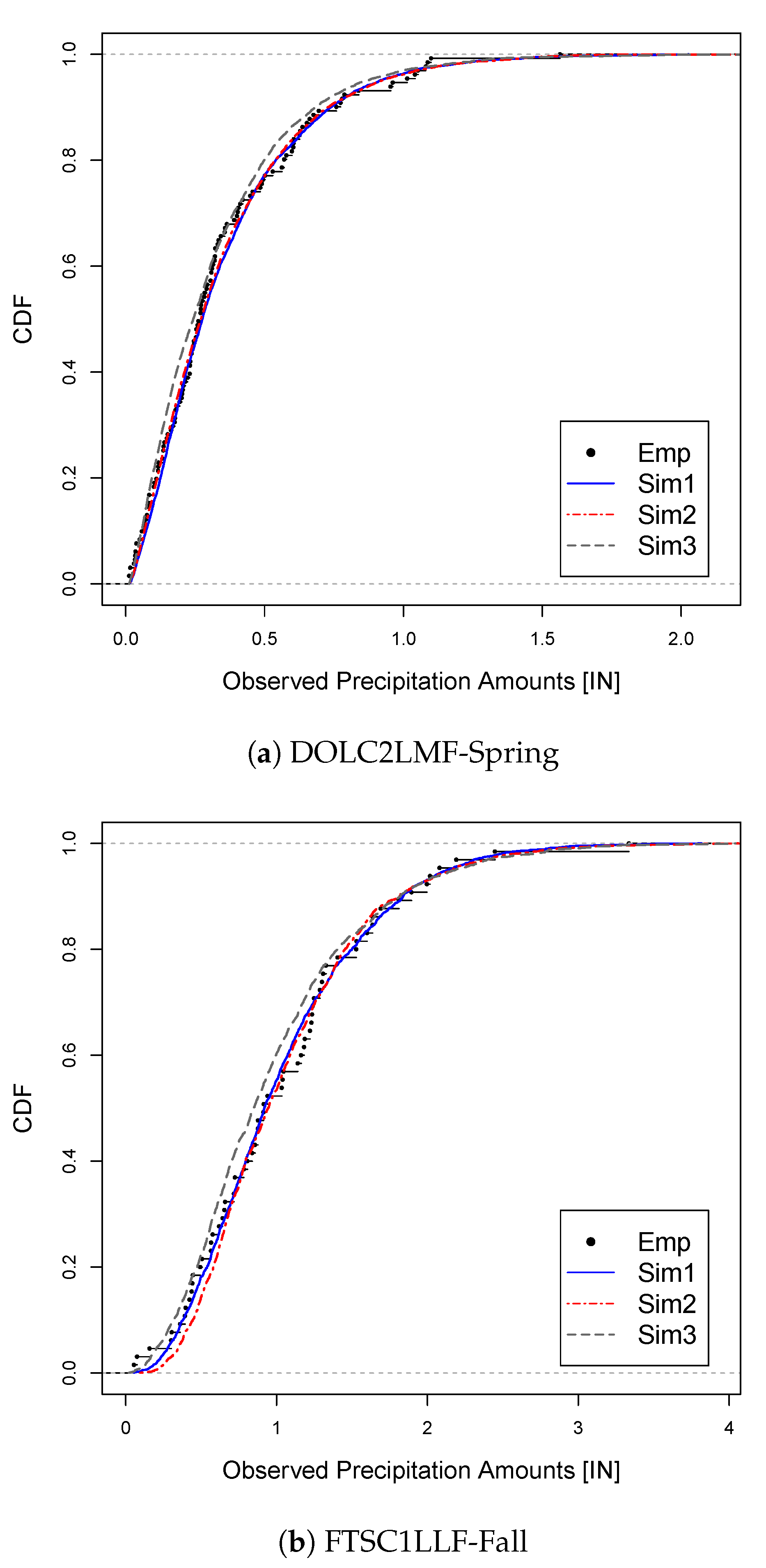
As discussed previously, there are situations where the conditional distribution of the observed variable given the forecast in a certain range of its domain is of particular interest. In these situations, one may target this specific conditional distribution to achieve a better fit through model tuning, while recognizing that the dependence parameter tuned this way generally does not provide optimal values for the entire joint distribution. Here, the targeted conditional CDFs are the ones obtained with the observed variable conditioned on the corresponding forecast variable being greater than the 75th percentile. This conditional tuning is illustrated by Figure 3, which shows one-dimensional EMD (EMD1d) values for a sequence of values for the same combinations of drainage areas and seasons used in Figure 2. In the plots, the circles represent the EMD1d values at the corresponding values. The dots represent the smoothed EMD1d values. For all of the cases considered in this work, the optimal values for the minimized smoothed EMD1d values are given in Table 3 below. The effect of this localized optimization can be demonstrated by Figure 4. This figure shows one-dimensional conditional CDFs for the observed variable for DOLC2LMF-Spring (a) and FTSC1LLF-Fall (b). The conditional CDFs are obtained with the observed variable conditioned on the corresponding forecast variable being greater than the 75th percentile. In each plot, along with an empirical CDF, CDFs obtained from simulations using the methods of SPCC (sim3-gray), MEMD applied to the bivariate distributions as described above (sim2-red), and MEMD applied to only the conditional distributions (sim1-blue) are given. We can see that sim1 yields the best fit for both cases. Since the EMD measures the area between two one-dimensional CDFs (Section 2), this outcome demonstrates well the fact that minimizing the EMD amounts to minimizing this area.
Table 3 presents more results for tuning the BMGD for the one-dimensional conditional distributions given forecast values being greater than the 75th percentile. In the table, the values are obtained from the SPCC, MLE, MEMD2d (MEMD for the BMGD unconditionally), MEMD1d (MEMD for the conditional distribution), and MKSS (the minimum KSS for the conditional distribution). The associated EMD1d and KSS values are smoothed values. While the results are mixed and may seem perplexing, we highlight here the performance of the conditional tuning methods. For WALN6, comparing MEMD1d and MKSS with SPCC, MLE, and MEMD2d, we can see large percentage reductions in EMD1d and KSS for the Spring, Summer, and Winter. For other locations, the results are mixed in a complicated way. To have an objective assessment of the results, we count the number of cases that one method outperforms another. Specifically, to compare a given pair of methods, e.g., MKSS and SPCC, we form a ratio of the number of cases that MKSS outperforms SPCC to the number of cases the MKSS underperforms the SPCC. The performance ratios are tabulated in Table 4. For MKSS vs. SPCC, the ratio in EMD1d is found to be 13:0 in the row with MKSS and SPCC appearing under EMD1d. We can see that the unconditional tuning method MEMD2d outperforms the SPCC considerably as measured by the ratios, but not so much for MEMD2d vs. MLE. The effect of the conditional tuning is much greater than that of the unconditional tuning as the ratios for the MEMD1d and MKSS indicate. Of course, when the choice of tuning (optimization) criterion is EMD1d, it is necessary that the MEMD1d outperforms the other methods. This is true also for MKSS. What is interesting here is that the ratios under KSS compellingly favor the MEMD1d and those under EMD1d favor the MKSS. The results suggest that, when the dependence parameter is optimized for a targeted conditional distribution, the GOF of the conditional distribution can be improved.
5. Discussion and Concluding Remarks
Precipitation is intermittent. In order to model the joint distribution between two variables of precipitation amounts, a mixed-type bivariate distribution is considered in this paper. A new proof for an intermittency equation of the model is given. With the use of an embedded bivariate meta-Gaussian distribution, this modeling approach allows for an explicit treatment of precipitation intermittency as well as a wide choice of parametric and non-parametric models for the marginal distributions. The focus of this work is on the question of whether and how the bivariate meta-Gaussian distribution can be tuned to yield an optimal fit. The meta-Gaussian distribution can be formulated in two different ways. In the conventional formulation, a normality assumption is needed. In certain real-world applications, however, this assumption may not hold. The second formulation, starting from a copula setup, forgoes this assumption and thus allows for model tuning. In this study, predicted single-valued precipitation amounts for a river basin area constitute one variable, and the corresponding observed precipitation amounts the other. The study of this modeling approach is motivated by a need to quantify the uncertainty in the single-valued precipitation forecasts in certain hydrometeorologic applications. In this setting, the uncertainty can be quantified by the conditional distributions given the forecasts.
Numerical simulations are carried out using real-world data from the Global Ensemble Forecast System of the U.S. National Centers for Environmental Prediction and four U.S. National Weather Service River Forecast Centers. The parameter in the meta-Gaussian distribution that characterizes the dependence of the two marginals is tuned under the Mallows distance for the entire joint distribution to yield an optimal value. The results obtained from this optimization are compared with the results obtained from using the sample correlation coefficient and maximum likelihood estimate as parameter values. It is found that the sample correlation coefficient and maximum likelihood estimate produce similar results for all the cases studied. Additionally, for three-fourths of the cases, results yielded by the sample correlation coefficient and the minimum Mallows distance are very close. These results suggest that tuning this dependence parameter has limited effects in altering the behaviour of the meta-Gaussian distribution model toward a better overall model fit.
It is known that the statistical relationship between a precipitation forecast variable and its corresponding observed variable can be nonlinear and heteroscedastic. Specifically, heteroscedasticity here refers to the situation in which the variance of the observed precipitation amounts changes over the range of the forecast precipitation amounts. The dependence parameter values determined from the conventional methods can be thought of as a middle-ground for balancing the fit across this range. When the meta-Gaussian distribution model for precipitation amounts is applied in predicting floods, goodness-of-fit (GOF) for the heavy precipitation amounts in the modeling has a larger impact than that for the light precipitation amounts, which entails a dependence parameter value tuned for the heavy precipitation amounts. This important aspect is investigated by applying the Mallows distance and the Kolmogorov–Smirnov statistic to finding an optimal dependence parameter value for the conditional distribution given the forecast greater than the 75th percentile of the forecast values. The results suggest that, when the dependence parameter is optimized for a targeted conditional distribution, the GOF of the conditional distribution can be improved.
Funding
This work was partially funded by the Advanced Hydrologic Prediction Service (AHPS) program of the National Weather Service (NWS), and by the Climate Predictions Program for the Americas (CPPA) of the Climate Program Office (CPO), both from the National Oceanic and Atmospheric Administration (NOAA). This support is gratefully acknowledged.
Acknowledgments
The author would like to thank the editors and referees for their valuable comments that lead to improved content and clarity of this work. Special thanks go to Yu Zhang of the NWS Office of Prediction for helpful suggestions.
Conflicts of Interest
The author declares no conflict of interest. The funders had no role in the design of the study; in the collection, analyses, or interpretation of data; in the writing of the manuscript, and in the decision to publish the results.
Appendix A
Equation (7) is used in the simulation study of this work. A derivation of this equation is included below for completeness. The derivation is different than the one given in [35]. We start with the density function of (6), denoted here by :
where , , , and are the density functions corresponding to , , , and , respectively. From Equation (6), by definition, we have:
It follows that has the density given in (A1).
Indeed, from density function (A1), by definition, we have:
Appendix B
A derivation of Equation (15) using calculus and elementary probability theory is given here. Assume . The conditional distribution is, by definition, the following limit:
where , . Now can be decomposed as:
Using Bayes’ Theorem, the second term of the right-hand side of this equation can be expressed as
It follows that (A4) can be written as
The denominator of the right-hand side of (A8) can be written as
Applying the steps used to obtain (A4)–(A6) to the first term and then the second term of the above equation, we have
where is the density function associated with defined in Section 3, and is a point in (First, mean value theorem for integration). Similarly, we can obtain the following equation for in (A8):
where is the density corresponding to defined in Section 3 and is in . It follows that
To obtain , it remains to show that
where is the density corresponding to defined in Section 3. Indeed, we have
Now, we assume that , , and are continuous. Then, the above equation is differentiable on both sides, which implies (A10).
References
- Kelly, K.S.; Krzysztofowicz, R. A bivariate meta-Gaussian density for use in hydrology. Stoch. Hydrol. Hydraul. 1997, 11, 17–31. [Google Scholar] [CrossRef]
- Krzysztofowicz, R.; Kelly, K.S. A Meta-Gaussian Distribution with Specified Marginals; Technical Report; University of Virginia: Charlottesville, VA, USA, 1996. [Google Scholar]
- Li, W.; Duan, Q.; Ye, A.; Miao, C. An improved meta-Gaussian distribution model for post-processing of precipitation forecasts by censored maximum likelihood estimation. J. Hydrol. 2019, 574, 801–810. [Google Scholar] [CrossRef]
- Schaake, J.C.; Demargne, J.; Hartman, R.; Mullusky, M.; Welles, E.; Wu, L.; Herr, H.; Fan, X.; Seo, D.-J. Precipitation and temperature ensemble forecasts from single-value forecasts. Hydrol. Earth Syst. Sci. Discuss. 2007, 4, 655–717. [Google Scholar] [CrossRef]
- Wu, L.; Seo, D.-J.; Demargne, J.; Brown, J.D.; Cong, S.; Schaake, J.C. Generation of ensemble precipitation forecast from single-valued quantitative precipitation forecast for hydrologic ensemble prediction. J. Hydrol. 2011, 399, 281–298. [Google Scholar] [CrossRef]
- Ye, A.; Deng, X.; Ma, F.; Duan, Q.; Zhou, Z.; Du, C. Integrating weather and climate predictions for seamless hydrologic ensemble forecasting: A case study in the Yalong river basin. J. Hydrol. 2017, 547, 196–207. [Google Scholar] [CrossRef]
- Papalexiou, S.M.; Koutsoyiannis, D. Entropy based derivation of probability distributions: A case study to daily rainfall. Adv. Water Resour. 2012, 45, 51–57. [Google Scholar] [CrossRef]
- Herr, H.D.; Krzysztofowicz, R. Generic probability distribution of rainfall in space: The bivariate model. J. Hydrol. 2005, 306, 234–263. [Google Scholar] [CrossRef]
- Serinaldi, F. Copula-based mixed models for bivariate rainfall data: An empirical study in regression perspective. Stoch Env. Res Risk Assess 2009, 23, 677–693. [Google Scholar] [CrossRef]
- Shimizu, K. A bivariate mixed lognormal distribution with an analysis of rainfall data. J. Appl. Meteorol. 1993, 32, 161–171. [Google Scholar] [CrossRef] [Green Version]
- Kedem, B.; Chiu, L.S.; North, G.R. Estimation of mean rain rate: Application to satellite observations. J. Geophys. Res. 1990, 95, 1965–1972. [Google Scholar] [CrossRef]
- Bowers, M.C.; Tung, W.M.; Gao, J.B. On the distributions of seasonal river flows: Lognormal or power law? Water Resour. Res. 2012, 48, W05536. [Google Scholar] [CrossRef]
- Demargne, J.; Wu, L.; Regonda, S.K.; Brown, J.D.; Haksu, L.; He, M.; Seo, D.-J.; Hartman, R.; Herr, H.D.; Fresch, M.; et al. The Science of NOAA’s Operational Hydrologic Ensemble Forecast Service. Bull. Am. Meteor. Soc. 2014, 95, 79–98. [Google Scholar] [CrossRef]
- Brown, J.D.; Wu, L.; He, M.; Regonda, S.; Haksu, L.; Seo, D.-J. Verification of temperature, precipitation, and streamflow forecasts from the NOAA/NWS Hydrologic Ensemble Forecast Service (HEFS): 1. Experimental design and forcing verification. J. Hydrol. 2014, 519, 2869–2889. [Google Scholar] [CrossRef]
- Brown, J.D.; He, M.; Regonda, S.; Wu, L.; Haksu, L.; Seo, D.-J. Verification of temperature, precipitation, and streamflow forecasts from the NOAA/NWS Hydrologic Ensemble Forecast Service (HEFS): 2. Streamflow verification. J. Hydrol. 2014, 519, 2847–2868. [Google Scholar] [CrossRef]
- Fang, H.-B.; Fang, K.-T.; Kotz, S. The meta-elliptical distributions with given marginals. J. Multivar. Anal. 2002, 82, 1–16. [Google Scholar] [CrossRef] [Green Version]
- Genest, C.; Favre, A.-C.; Beliveau, J.; Jacques, C. Metaelliptical copulas and their use in frequency analysis of multivariate hydrological data. Water Resour. Res. 2007, 43, W09401. [Google Scholar] [CrossRef] [Green Version]
- Jolliffe, I.T.; Stephenson, D.B. Forecast Verification: A Practitioner’s Guide in Atmospheric Science. In Atmospheric Science; Jolliffe, I.T., Stephenson, D.B., Eds.; John Wiley and Sons: Chichester, UK, 2003. [Google Scholar]
- Meyer, C. The Bivariate Normal Copula. Commun. Stat. Theory Methods 2013, 42, 2402–2422. [Google Scholar] [CrossRef] [Green Version]
- Sklar, A. Random Variables, Joint Distribution Functions, and Copulas. Kybernetika 1973, 9, 449–460. [Google Scholar]
- Bouyé, E.; Salmon, M. Dynamic copula quantile regressions and tail area dynamic dependence in Forex markets. Eur. J. Financ. 2009, 15, 721–750. [Google Scholar] [CrossRef]
- Rohatgi, V.K.; Ehsanes Saleh, A.K.M. Section 8.7, Maximum likelihood estimators, Theorem 4. In An Introduction to Probability Theory and Mathematics, 2nd ed.; John Wiley and Sons: Hoboken, NJ, USA, 1976. [Google Scholar]
- Joe, H. Asymptotic efficiency of the two-stage estimation method for copula-based models. J. Multivar. Anal. 2005, 94, 401–419. [Google Scholar] [CrossRef] [Green Version]
- Storvik, B.; Storvik, G.; Fjortoft, R. On the Combination of Multisensor Data Using Meta-Gaussian Distributions. IEEE Trans. Geosci. Remote Sens. 2009, 47, 2372–2379. [Google Scholar] [CrossRef]
- Levina, E.; Bickel, P.J. The Earth Mover’s Distance is the Mallows Distance: Some Insights from Statistics. In Proceedings of the Eighth IEEE International Conference on Computer Vision, ICCV 2001, Vancouver, BC, Canada, 7–14 July 2001; pp. 251–256. [Google Scholar]
- Thorarinsdottir, T.L.; Gneiting, T.; Gissibl, N. Using Proper Divergence Functions to Evaluate Climate Models. SIAM/ASA J. Uncertain. Quantif. 2013, 1, 522–534. [Google Scholar] [CrossRef] [Green Version]
- Zhou, D.; Shi, T. Statistical inference based on distances between empirical distributions with applications to airslevel-3 data. In Proceedings of the 2011 NASA Conference on Intelligent Data Understanding, Mountain View, CA, USA, 19–21 October 2011; pp. 129–143. [Google Scholar]
- Rubner, Y.; Tomasi, C.; Guibas, L.J. The Earth Mover’s Distance as a Metric for Image Retrieval. Int. J. Comput. Vis. 2000, 40, 99–121. [Google Scholar] [CrossRef]
- Trenberth, K.E.; Zhang, Y.; Gehne, M. Intermittency in Precipitation: Duration, Frequency, Intensity, and Amounts Using Hourly Data. J. Hydrometeorol. 2017, 18, 1393–1412. [Google Scholar] [CrossRef] [Green Version]
- Li, C.; Singh, V.P.; Mishra, A.K. A bivariate mixed distribution with a heavy-tailed component and its application to single-site daily rainfall simulation. Water Resour. Res. 2013, 49, 767–789. [Google Scholar] [CrossRef] [Green Version]
- Herr, H.D. A Bivariate Precipitation Uncertainty Processor for Probabilistic River Forecasting. Master’s Thesis, University of Virginia, Charlottesville, VA, USA, 1999; pp. 24–31. [Google Scholar]
- Seo, D.-J.; Breidenbach, J.P. Real-time correction of spatially nonuniform bias in radar rainfall data using rain gauge measurements. J. Hydrometeorol. 2002, 3, 93–111. [Google Scholar] [CrossRef] [Green Version]
- Hamill, T.M.; Bates, G.T.; Whitaker, J.S.; Murray, D.R.; Fiorino, M.; Galarneau, T.J.; Zhu, Y.; Lapenta, W. NOAA’s SecondGeneration Global MediumRange Ensemble Forecast Dataset. Bull. Am. Meteor. Soc. 2013, 94, 1553–1565. [Google Scholar] [CrossRef]
- Jones, P.W. First- and second-order conservative remapping schemes for grids in spherical coordinates. Mon. Weather Rev. 1999, 127, 2204–2210. [Google Scholar] [CrossRef]
- Li, C.; Singh, V.P.; Mishra, A.K. Simulation of the entire range of daily precipitation using a hybrid probability distribution. Water Resour. Res. 2012, 48, W03521. [Google Scholar] [CrossRef]
Figure 1.
Scatter plots of the transformed forecast and observed.

Figure 2.
EMD values for the methods of SPCC, MLE, and MEMD.

Figure 3.
EMD values as a function of for.


Figure 4.
The conditional empirical CDF and its simulated CDFs.


Table 1.
Drainage area centroids and corresponding GEFS grid points.
| Centroid | Grid Point | |||
|---|---|---|---|---|
| Lon (W) | Lat (N) | Lon (W) | Lat (N) | |
| BLKO2 | 97.28 | 36.81 | 97.50 | 37.22 |
| DOLC2LMF | 108.22 | 37.63 | 108.28 | 37.69 |
| FTSC1LLF | 123.15 | 39.60 | 123.28 | 39.56 |
| WALN6 | 75.14 | 42.17 | 75.00 | 42.37 |
Table 2.
EMD between the empirical bivariate CDF and its simulated CDFs.
| Spring | Summer | Fall | Winter | ||
|---|---|---|---|---|---|
| EMD | EMD | EMD | EMD | ||
| BLKO2 | SPCC | 0.62 0.057 | 0.36 0.049 | 0.59 0.078 | 0.77 0.041 |
| MLE | 0.66 0.059 | 0.41 0.049 | 0.59 0.076 | 0.81 0.041 | |
| MEMD | 0.62 0.057 | 0.40 0.049 | 0.77 0.062 | 0.78 0.041 | |
| DOLC2LMF | SPCC | 0.38 0.028 | 0.32 0.024 | 0.31 0.030 | 0.40 0.031 |
| MLE | 0.39 0.026 | 0.34 0.024 | 0.35 0.029 | 0.43 0.029 | |
| MEMD | 0.46 0.024 | 0.35 0.024 | 0.36 0.028 | 0.51 0.028 | |
| FTSC1LLF | SPCC | 0.77 0.049 | 0.58 0.083 | 0.77 0.066 | 0.80 0.073 |
| MLE | 0.79 0.046 | 0.65 0.076 | 0.79 0.063 | 0.82 0.068 | |
| MEMD | 0.85 0.042 | 0.62 0.074 | 0.87 0.061 | 0.86 0.062 | |
| WALN6 | SPCC | 0.70 0.032 | 0.49 0.036 | 0.72 0.035 | 0.82 0.035 |
| MLE | 0.72 0.032 | 0.51 0.036 | 0.74 0.029 | 0.84 0.035 | |
| MEMD | 0.74 0.031 | 0.62 0.030 | 0.77 0.027 | 0.78 0.033 |
Table 3.
Results for conditional tuning.
| Spring | Summer | Fall | Winter | ||
|---|---|---|---|---|---|
| EMD1d KSS | EMD1d KSS | EMD1d KSS | EMD1d KSS | ||
| BLKO2 | SPCC | 0.62 0.069 0.084 | 0.36 0.072 0.077 | 0.59 0.169 0.107 | 0.77 0.102 0.117 |
| MLE | 0.66 0.053 0.067 | 0.41 0.072 0.071 | 0.59 0.169 0.107 | 0.81 0.079 0.094 | |
| MEMD2d | 0.62 0.069 0.084 | 0.40 0.070 0.070 | 0.77 0.108 0.126 | 0.78 0.095 0.112 | |
| MEMD1d | 0.68 0.049 0.068 | 0.39 0.069 0.070 | 0.72 0.090 0.113 | 0.89 0.072 0.087 | |
| MKSS | 0.66 0.053 0.067 | 0.38 0.070 0.068 | 0.67 0.119 0.075 | 0.87 0.076 0.083 | |
| DOLC2LMF | SPCC | 0.38 0.031 0.096 | 0.32 0.018 0.066 | 0.31 0.037 0.089 | 0.40 0.055 0.087 |
| MLE | 0.39 0.029 0.094 | 0.34 0.021 0.074 | 0.35 0.033 0.072 | 0.43 0.048 0.094 | |
| MEMD2d | 0.46 0.018 0.061 | 0.35 0.023 0.076 | 0.36 0.033 0.067 | 0.51 0.042 0.141 | |
| MEMD1d | 0.46 0.018 0.059 | 0.28 0.018 0.053 | 0.40 0.029 0.066 | 0.51 0.042 0.120 | |
| MKSS | 0.49 0.019 0.058 | 0.29 0.018 0.053 | 0.37 0.032 0.063 | 0.39 0.055 0.085 | |
| FTSC1LLF | SPCC | 0.77 0.108 0.097 | 0.58 0.110 0.177 | 0.77 0.083 0.109 | 0.80 0.067 0.042 |
| MLE | 0.79 0.096 0.094 | 0.65 0.096 0.150 | 0.79 0.069 0.104 | 0.82 0.066 0.047 | |
| MEMD2d | 0.85 0.077 0.081 | 0.62 0.104 0.149 | 0.87 0.058 0.090 | 0.86 0.102 0.071 | |
| MEMD1d | 0.84 0.074 0.085 | 0.70 0.087 0.159 | 0.84 0.052 0.092 | 0.82 0.066 0.044 | |
| MKSS | 0.84 0.074 0.079 | 0.63 0.102 0.147 | 0.85 0.054 0.088 | 0.80 0.067 0.042 | |
| WALN6 | SPCC | 0.70 0.067 0.099 | 0.49 0.094 0.164 | 0.72 0.076 0.127 | 0.82 0.054 0.161 |
| MLE | 0.72 0.060 0.094 | 0.51 0.088 0.154 | 0.74 0.073 0.113 | 0.84 0.049 0.148 | |
| MEMD2d | 0.74 0.053 0.094 | 0.62 0.044 0.088 | 0.77 0.062 0.093 | 0.78 0.067 0.197 | |
| MEMD1d | 0.84 0.035 0.077 | 0.70 0.026 0.066 | 0.80 0.059 0.082 | 0.94 0.023 0.067 | |
| MKSS | 0.85 0.036 0.073 | 0.68 0.028 0.064 | 0.81 0.062 0.075 | 0.94 0.023 0.063 |
Table 4.
Performance ratios.
| EMD1d | KSS | ||
|---|---|---|---|
| MEMD2d | SPCC | 12:3 | 11:4 |
| MLE | 9:6 | 8:7 | |
| MEMD1d | SPCC | 15:0 | 13:3 |
| MLE | 15:0 | 12:4 | |
| MEMD2d | 14:0 | 12:3 | |
| MKSS | SPCC | 13:0 | 15:0 |
| MLE | 12:3 | 15:0 | |
| MEMD2d | 11:3 | 16:0 |
© 2020 by the author. Licensee MDPI, Basel, Switzerland. This article is an open access article distributed under the terms and conditions of the Creative Commons Attribution (CC BY) license (http://creativecommons.org/licenses/by/4.0/).
Share and Cite
MDPI and ACS Style
Wu, L. Tuning the Bivariate Meta-Gaussian Distribution Conditionally in Quantifying Precipitation Prediction Uncertainty. Forecasting 2020, 2, 1-19. https://0-doi-org.brum.beds.ac.uk/10.3390/forecast2010001
AMA Style
Wu L. Tuning the Bivariate Meta-Gaussian Distribution Conditionally in Quantifying Precipitation Prediction Uncertainty. Forecasting. 2020; 2(1):1-19. https://0-doi-org.brum.beds.ac.uk/10.3390/forecast2010001
Chicago/Turabian StyleWu, Limin. 2020. "Tuning the Bivariate Meta-Gaussian Distribution Conditionally in Quantifying Precipitation Prediction Uncertainty" Forecasting 2, no. 1: 1-19. https://0-doi-org.brum.beds.ac.uk/10.3390/forecast2010001