X-Model: Further Development and Possible Modifications

Abstract

The main goal of the present paper is to improve the X-model used for day-ahead electricity price and volume forecasting. The key feature of the X-model is that it makes a day-ahead forecast for the entire wholesale supply and demand curves. The intersection of the predicted curves yields the forecast for equilibrium day-ahead prices and volumes. We take advantage of a technique for auction curves’ transformation to improve the original X-model. Instead of using actual wholesale supply and demand curves, we rely on transformed versions of these curves with perfectly inelastic demand. As a result, the computational requirements of our X-model are reduced and its forecasting power increases. Moreover, our X-model is more robust towards outliers present in the initial auction curves’ data.

1. Introduction

Due to the fact that electricity markets are becoming increasingly more competitive, many participants of these markets seek to optimize their trading strategies and minimize their risk exposure. As a result, the field of electricity price forecasting has developed considerably over the past decades. Following [1], a large amount of methods has been created to solve a variety of forecasting problems. These methods are based on a wide range of possible modeling approaches and thus have their particular advantages and disadvantages.

Predicting price spikes has proven to be one of especially important issues in the field of electricity price forecasting. These low-probability and high-impact events not only influence bidding strategies of market participants, but also affect electricity production and consumption schedules. As a result, many forecasting models were designed with the aim to capture these price spikes well. In fact, relevant for the present paper are two groups of price forecasting models: time series-based and structural ones.

The former group can be represented by ARX-type models standard in electricity price forecasting. The latest iterations of these models were described in, e.g., [2] or [3] for day-ahead and intraday electricity markets. Moreover, GARCH-type models as in, e.g., [4,5] or [6] have proven to be suitable for the forecasting of price spikes in the Spanish, Italian, and U.K. markets, respectively. Jump diffusion models (as in, e.g., [7,8,9], or [10]) and regime switching models (see, e.g., [11,12,13,14], or [15]) have also been applied successfully to predict electricity prices in a variety of settings.

On the other hand, the family of models in the latter group is extensive and more diverse. To keep the literature review concise, the focus will be placed on models that study supply and demand curves in an electricity market. The work in [16] described the price process in the Alberta and California markets using the real-world auction data. The work in [17] conducted a study of Californian electricity prices by taking advantage of latent supply and demand curves. To estimate the curves, the authors of the paper relied on temperature data, seasonality factors, and gas availability. Models by, e.g., [18,19] followed a more functional approach and were driven by real auction curves’ data. Moreover, there exists a field of more structural approaches to modeling the auction curves. For example, the work in [20,21] use bid stacks to determine electricity spot prices on the basis of power demand and prices of generating fuels.

However, time series-based models typically neglect fundamental dependencies present in the electricity market. In turn, structural models usually do not take substantial advantage of the underlying historical data. A model that bridges the gap is the so-called X-model developed by [22]. More specifically, the X-model uses a time series-based approach to make a prediction for entire day-ahead wholesale supply and demand curves. The intersection of the predicted auction curves yields a forecast for equilibrium prices and volumes. It follows that the X-model includes the properties of both time series and structural analyses.

More importantly, there have been many advances in the field of modeling of wholesale supply and demand curves in electricity markets. For example, the work in [23] proposed another functional approach to model the wholesale supply and demand curves. Using the example of the Italian electricity market, the authors of the paper suggested to treat each curve as a single structured object in a functional space and use the autocorrelation between the curves to conduct a forecast for the entire curves. A similar functional model (albeit only a parametric one) was developed in [24] and was applied to the Italian gas market. The work in [25] measured the influence of clean energies on electricity prices in the German market. In doing so, the model in [25] added or subtracted amounts of renewable supply from the initial auction curves’ data. As a result, the model shifted the wholesale auction curves to produce results. A similar approach was followed by [26] who studied the impact of errors in renewable energy forecasts on intraday electricity prices. The work in [26] obtained the results by shifting the day-ahead auction curves to approximate the intraday auction curves. The work in [27] relied on the findings of [28] to manipulate the observed wholesale auction curves and derive a fundamental model of the German electricity market.

The present paper extends the field of modeling of the wholesale auction curves and provides presumably the first improvement of the X-model. More specifically, the paper is based on the concept elaborated by [19]. Following this concept, it is possible to transform initial wholesale auction curves into their analogues with perfectly inelastic demand. Important is the fact that the equilibrium price is the same before and after the transformation. We show that using the X-model on the transformed auction curves, i.e., predicting the transformed day-ahead wholesale supply and demand curves instead of the original ones, allows the forecasting accuracy of the X-model to be improved and its computational burden to be decreased. Moreover, the improved X-model becomes more robust towards outliers present in the initial auction curves’ data.

The paper has the following structure. The remainder of the present section discusses the paper by [19] and comments on the main idea of the present paper. Section 2 is divided into three subsections. The first one provides institutional details of the German day-ahead wholesale market; the second one comments on data sources; and the third one discusses data filtering. Section 3 is devoted to the methodology. This section first provides a detailed general description of the modified X-model and then elaborates on steps for developing the model. Section 4 presents the obtained results. Section 5 concludes the paper and discusses possibilities for further research.

Main Idea

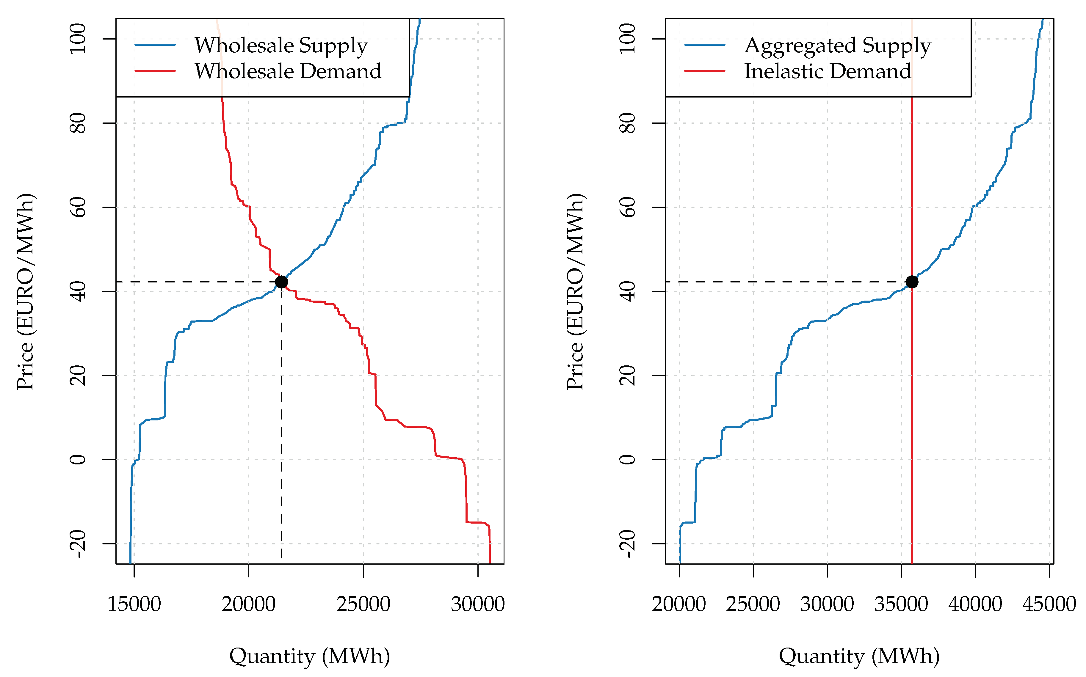
As was mentioned earlier, the concept of the wholesale auction curves’ transformation described in [19] lies in the core of the present paper. An application of the concept to day-ahead wholesale supply and demand curves observed in the German electricity market is presented in Figure 1.

The intuition behind the concept is based on the fact that, besides the wholesale market, there exists a bilateral market for electricity trading. Electricity producers and consumers are directly connected with each other in this market. Therefore, if prices in the bilateral market are higher than prices in the wholesale market, some electricity suppliers decide to abstain from the production of electricity. Instead, they try to buy electricity in the wholesale market. Hence, the wholesale demand curve is elastic because some market participants are sensitive to the wholesale market price. However, if we assume that electricity suppliers cannot use wholesale arbitrage opportunities, only a few market participants actually are price sensitive.

Thus, as [19] suggested, the existence of two parallel markets complicates the process of electricity markets’ modeling. To avoid complications, the work in [19] proposed to assume that all orders in the wholesale demand curve were of an arbitrage nature. Under this assumption, it is possible to shift all wholesale demand elasticities to the supply side. As a result, the demand curve turns inelastic. Moreover, equilibrium volume increases because the transformed supply curve incorporates the shifted demand orders. The equilibrium price, however, remains unchanged. Therefore, the transformed auction curves better reflect the fundamental market equilibrium because they take into account the existence of arbitrage orders.

There are two key benefits of the modified X-model with the transformed auction curves relative to the original X-model. First, predicting only one point instead of the entire demand curve requires a much smaller amount of computational time. Second, the modified X-model is less dependent on outliers present in the original auction curves’ data. This holds because outliers can occur in each segment of the wholesale demand curve. The forecast of the wholesale demand can thus accumulate these outliers and lose its accuracy. On the contrary, the forecast of the inelastic demand cannot be affected by such a cumulative effect. Therefore, outliers in the initial auction curves influence the original X-model more than the modified one. As a result, the modified X-model yields more precise results.

2. Data

2.1. Institutional Details of the German Electricity Market

The EPEX SPOR SE runs several electricity trading auctions in the German bidding zone. The timing of these auctions and their detailed description is provided in, e.g., [29] or [30]. The focus of the present paper will be placed on the day-ahead auction for hourly products. This auction takes place on a daily basis at 12:00 a day prior to the day of delivery. Market participants submit their bids to a system that acts as an auctioneer and establishes 24 equilibrium prices for the following day. To determine these prices, the system draws 24 combinations of day-ahead wholesale supply and demand curves on the grounds of the submitted bids. The intersections of the curves coincide with the announced prices. In turn, the prices are revealed as soon as possible starting at 12:42 on the day the auction clears. The maximal bid price in the German day-ahead market is equal to $P_{max}=3000$, and the lowest bidding price amounts to $P_{min}=-500$.

Besides the day-ahead auction, several other trading venues exist in the German electricity market. Among them are continuous and non-continuous intraday markets for hourly and quarter-hourly products. The balancing market exists to account for discrepancies between final electricity supply and demand volumes. Furthermore, in addition to the wholesale market, electricity is also traded via OTCcontracts.

2.2. Data Description

The present study was conducted on the day-ahead wholesale auction curves’ data from the German EPEX SPOT SE (see [31,32]). An example of the observed curves is illustrated on the left-hand side of Figure 1. It is important that the auction curves are constructed by aggregating price-volume combinations submitted by market participants to the electricity exchange. To ease further notation, we denote the bid volume at price $P_{min}$ in the supply curve as $Y_{d,h}^{S,1}$ and the ask volume at price $P_{max}$ in the demand curve as $Y_{d,h}^{D,1}$ where d and h are time indices. Thus, to build the supply curve at time point $(d,h)$, volume $Y_{d,h}^{S,1}$ is first taken as a starting point. The bid volumes at prices $(P_{min},P_{max}]$ are then one-by-one added as increments to $Y_{d,h}^{S,1}$ to draw the supply curve. The demand curve at $(d,h)$ is then constructed analogously. Volume $Y_{d,h}^{D,1}$ is taken as a starting point, and ask volumes at prices $(P_{max},P_{min}]$ are incremented one-by-one to $Y_{d,h}^{D,1}$ to finalize the demand curve.

Additional datasets were obtained from the ENTSOE(see [33]). These datasets included wind and solar power forecasts and total load forecast. The in-sample period extended from 2016-01-01 to 2017-01-01. The out-of-sample period was the year 2017. The data were clock-change adjusted. The missing hours in March were calculated using the two values before and after them. The average value of the two double hours in October was taken to account for the clock-change.

2.3. Data Filtering

There were two clusters of outliers present in the original data. The first cluster was detected in $Y^{S,1}$ time series, the second one in $Y^{D,1}$. The fact that these clusters are outliers becomes apparent given that, e.g., observations $Y_{d,h}^{S,\gamma }$ and $Y_{d,h}^{D,\gamma }$ at prices $P_S^1=P_{min}+5$ and $P_D^1=P_{max}-5$, respectively, did not have any peculiarities. For instance, the volume size $Y_{d,h}^{S,1}$ in the starting point of the supply curve at time point 2016-04-01 00:00:00 equals 316 (MWh), and the corresponding volume size $Y_{d,h}^{S,\gamma }$ at $P_S^1$ amounts to 16,904.77 (MWh). Naturally, only the latter number corresponds to a realistic order size posted by a market participant. In total, 252 outlier observations were clustered between 2016-03-31 22:00:00 and 2016-05-18 00:00:00 in the values of $Y^{S,1}$, and 845 outlier observations were clustered in between 2016-04-01 07:00:00 and 2016-05-20 20:00:00 in the values of $Y^{D,1}$. No observations outside of these clusters exhibited outlier behavior. Hence, from an economic standpoint, it is possible that market participants tried to bid unrealistic volumes at the extremes of the auction curves in the hope to get very profitable deals.

Please note that these outliers influence the functioning of the X-model. This happens because they lie in the starting points $Y_{d,h}^{S,1}$ and $Y_{d,h}^{D,1}$ of the auctions curves. As was mentioned in the previous subsection, the auction curves are constructed by incrementing volumes over the starting points $Y_{d,h}^{S,1}$ and $Y_{d,h}^{D,1}$ of the curves, i.e., by adding volumes at prices $(P_{min},P_{max}]$ to the volume sizes at $P_{min}$ and $P_{max}$ for the supply and demand curves, respectively. Therefore, if the volume forecasts for the starting points are influenced by outliers, the predictions for the entire curves, too, will be affected. In other words, if the outliers are not processed correctly, the forecasted supply and demand curves are shifted away from the true equilibrium because volumes at prices $(P_{min},P_{max}]$ are incremented over wrongly predicted starting points. Furthermore, it is technically possible to directly use volumes $Y_{d,h}^{S,\gamma }$ and $Y_{d,h}^{D,\gamma }$ as starting points to construct the auction curves. The performance of the model will not be greatly reduced in this case because equilibrium prices almost never reach their extremes at $P_{min}$ or $P_{max}.$

To clean the outliers, a method proposed by [34] was used. A typical expert-type regression model similar to [35] or [36] was constructed. The model has the following specification:

$$\begin{array}{c}\hfill \begin{array}{c}\hfill Y_{d,h}^{C,1}={\left({\mathit{\beta }}_{d,h}^C\right)}^{\prime }{\mathit{Z}}_{d,h}^C+{\epsilon }_{d,h}^C\end{array}\end{array}$$

(1)

where d and h are time indices; $C=(S,D)$ denotes supply and demand curves, respectively; $Y_{d,h}^{C,1}$ stands for an electricity volume in the starting point of a curve; ${\mathit{\beta }}_{d,h}^C$ is a vector of regression coefficients and ${\mathit{Z}}_{d,h}^C=(1,Y_{d-1,h}^{C,1},Y_{d-2,h}^{C,1},Y_{d-7,h}^{C,1},{\mathrm{DoW}}_d^1,{\mathrm{DoW}}_d^6,{\mathrm{DoW}}_d^7,Y_{d,h}^{C,\gamma })$, where DoW denotes a weekday dummy. Thus, the outliers’ processing model includes lags of 1, 2, and 7 and Monday, Saturday, and Sunday dummies. Moreover, the model is extended with additional regressors represented by the values of $Y_{d,h}^{S,\gamma }$ and $Y_{d,h}^{D,\gamma }$ at points $P_S^1=P_{min}+5$ and $P_D^1=P_{max}-5$ for the supply and demand curves, respectively. Note that in a normal (non-outlier) case, the values of $Y_{d,h}^{S,\gamma }$ for the supply curve and $Y_{d,h}^{D,\gamma }$ for the demand curve are usually very close to $Y_{d,h}^{S,1}$ and $Y_{d,h}^{D,1}$, respectively. Therefore, including $Y_{d,h}^{S,\gamma }$ and $Y_{d,h}^{D,\gamma }$ in the outliers’ processing model allows the precision of the model to be improved substantially.

3. Methodology

3.1. General Description of the Modified X-Model

The X-model does not rely on equilibrium price and volume time series to carry out a day-ahead forecast of electricity prices or volumes. Instead, the X-model forecasts the entire day-ahead wholesale supply and demand curves. Since these curves are used to settle wholesale market prices, the intersection of the predicted curves yields a price or volume forecast. As was mentioned earlier, the modified version of the X-model is based on the transformed wholesale auction curves with perfectly inelastic demand. Therefore, the auction curves’ transformation as described in [19] is the first step to be undertaken.

Second, to make a prediction of the entire day-ahead supply curve at time period $t+1$, the model first selects several points on this curve. These points correspond to predefined price levels and in the original paper by [22] were referred to as price classes. The price classes are selected as follows. First, an average supply curve over T in-sample observations is computed. Then, $M_S$ prices are selected on this curve. The goal when choosing these prices is to ensure that that the horizontal distances between the selected price-volume combinations are identical. In other words, an equidistant volume grid is applied to the average supply curve to derive the price classes. Of course, the greater the number $M_S$ of the price classes is, the more accurate the forecast becomes, but the higher the computational burden of the model is. Furthermore, given that the demand curve is perfectly inelastic, there is only one price class on the demand side. Hence, $M_D=1$.

Third, historical volume sizes are recalled for each of the $M=M_S+M_D$ price classes. As a result, M time series with wholesale volumes at the corresponding price levels are drawn. A day-ahead forecasting model is then applied to each of the time series separately. As a result, the forecasts deliver $M_S$ price-volume combinations on the supply curve and an $M_D=1$ price-volume combination for the demand at $t+1$.

Then, the obtained volume forecasts for $t+1$ in each of the $M_S$ price classes are combined together (or, loosely speaking, connected with one another into one curve) to create a forecast for the entire supply curve at time period $t+1$. It is important that $M_S$ price-volume combinations are not connected with each other with $M_S-1$ straight lines. A more sophisticated method called supply curve reconstruction is used to retain the form and structure of the supply curve. Finally, the intersection between the predicted supply and demand curves is determined to produce the day-ahead price and volume forecasts at $t+1$.

3.2. Transformation of the Auction Curves

The first step in deriving the modified X-model is to transform the wholesale supply and demand curves. The formulas for the transformation are taken directly from [19]. To simplify our notation, we consider both auction curves as functions of the market price. The inelastic demand curve can thus be represented as:

$$\begin{array}{c}\hfill \begin{array}{c}\hfill De{m}_t^{inelastic}=WSDe{m}_t^{-1}\left(P_{max}\right)\end{array}\end{array}$$

(2)

where $WSDem$ is a function that denotes the demand curve in the wholesale market. The equation for the transformed supply curve reads:

$$\begin{array}{c}\hfill \begin{array}{c}\hfill Su{p}_t^{-1}\left(z\right)=WSSu{p}_t^{-1}\left(z\right)+WSDe{m}_t^{-1}\left(P_{min}\right)-WSDe{m}_t^{-1}\left(z\right)\end{array}\end{array}$$

(3)

where $WSSup$ is a function that denotes the supply curve in the wholesale market.

3.3. Defining the Price Classes

Having transformed the auction curves, it is possible to apply the X-model and carry out price and volume forecasts. Please note that the formulas below are almost identical to those in the original paper by [22] to ensure the comparability of the original and modified X-models. However, the applied transformation of the auction curves requires us to focus only on the supply side because the demand curve is represented by a single point. As a result, we can omit many indices in the formulas below. Hence, the less sophisticated appearance of the mathematical part of the present paper is another simplification of the original X-model.

To construct the X-model, we need to determine price classes on the transformed supply curve. The price classes, as has already been mentioned, are points on the supply curve that correspond to certain prices and to which volume forecasting models are applied. The price classes are selected by first computing an average supply curve over T in-sample observations. To obtain this curve, we need to define a grid of prices $\mathcal{P}$, which have at least one positive bid volume during the in-sample period. Thus, it holds that $\mathcal{P}=\{P\in \mathbb{P}|V_t\left(P\right)>0\}$ where $\mathbb{P}$ denotes a grid of all possible possible prices in the interval from $P_{min}$ to $P_{max}$ and V stands for volumes on curve $Su{p}_t^{-1}$. We then compute average volumes over T in-sample observations at prices $\mathcal{P}$ as:

$$\begin{array}{c}\hfill \begin{array}{c}\hfill \overline{V}\left(P\right)=\frac{1}{T}\sum _{t=1}^T{V}_t\left(P\right)\mathrm{where}P\in \mathcal{P}.\end{array}\end{array}$$

(4)

Given the above expression, writing the equation for average curve ${\overline{Sup}}_t^{-1}$ over the in-sample period yields:

$$\begin{array}{c}\hfill \begin{array}{c}\hfill {\overline{Sup}}^{-1}\left(P\right)=\sum _{\begin{array}{c}p\in \mathcal{P}\\ p\le P\end{array}}\overline{V}\left(p\right)\mathrm{where}P\in \mathcal{P}\end{array}\end{array}$$

(5)

Finally, we apply an equidistant volume grid with a step of $V_{*}=500$ mW to the inverse $\overline{Sup}\left(V\right)$ of curve ${\overline{Sup}}^{-1}\left(P\right)$. This allows us to define the price classes as $\mathcal{C}=\left\{\overline{Sup}\left(i{V}_{*}\right)\right|i\in \mathbb{N}\}.$ As a result, the application of the equidistant volume grid with the selected size of $V_{*}$ to the derived average supply curve $\overline{Sup}\left(V\right)$ yields $M_S=19$ price classes.

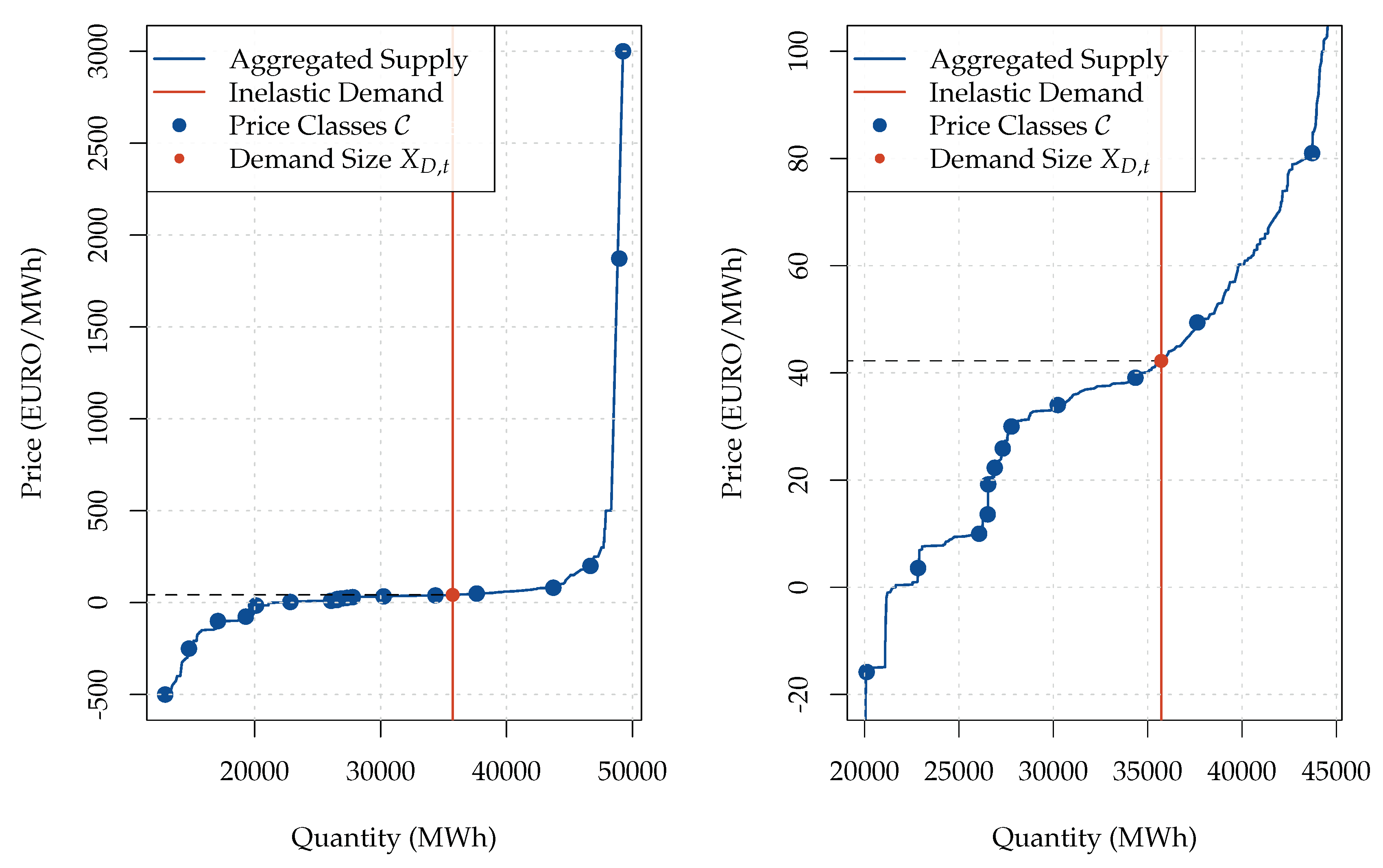
Of course, the method of applying an equidistant volume grid to the average supply curve may appear too simple for determining the price classes. However, despite its simplicity, the method proves to be relatively efficient. Following an example illustrated in Figure 2, it is clear that the number of price classes is greater in the flatter segments of the transformed supply curve and is smaller in the steeper segments. However, note that the equilibrium price is typically realized in the flatter segments of the supply curve. Therefore, using the equidistant volume grid allows us to focus on more important sectors of the supply curve without using any sophisticated techniques. Furthermore, there is no certain mathematical reason for choosing the size of $V_{*}$. The selected value of $V_{*}$ must allow us to obtain such an amount of price classes that their number is (a) sufficient enough for approximating the supply curve relatively precisely and (b) is not too large and is thus not computationally inefficient.

There were $M_S=16$ price classes in the original paper by [22]. Given that there is only one price class on the demand side in our case (as compared to $M_D=16$ in the original paper), we can use the spared computational time to select more price classes on the supply side and thus improve the quality of our supply forecast. The defined $M_S=19$ price classes $\mathcal{C}$ are provided in

Table 1. The defined $M_S=19$ price classes $\mathcal{C}$.

−500.0	−250.0	−100.1	−76.1	−15.8	3.6	10.0	13.6	19.2	22.3
25.9	30.0	34.0	39.1	49.4	81.0	200.0	1871.9	3000.0

.

Furthermore, we define volume size $X_{S,t}^{\left(c\right)}$ in price class $c\in \mathcal{C}$ as:

$$\begin{array}{c}\hfill \begin{array}{c}\hfill X_{S,t}^{\left(c\right)}=\sum _{P\in \mathcal{P}\left(c\right)}{V}_t\left(P\right)\mathrm{where}c\in \mathcal{C}\end{array}\end{array}$$

(6)

and the inelastic demand volume $X_{D,t}$ is given by:

$$\begin{array}{c}\hfill \begin{array}{c}\hfill X_{D,t}=De{m}_t^{inelastic}.\end{array}\end{array}$$

(7)

Thus, the total amount of variables that we need to forecast equals $M=M_S+M_D=20$.

Equation (6) has a critical implication for the functioning of the X-model. Note that volume $X_{S,t}^{\left(c\right)}$ incorporates the sum of the volumes present in between price classes c and $c-1$. Hence, as Section 2.2 suggests, the way the X-model builds the forecasted supply curve is similar to the way the actual wholesale supply curve is constructed. More specifically, volume $X_{S,t}^1$ in price class $c=1$ is taken as the starting point. The volumes in the following price classes $(2,\dots ,M_S)$ are added to the value of $X_{S,t}^1$ as increments to draw the entire supply curve.

The above description implies that outliers present in the initial supply curves’ data are accumulated in the forecast for the entire supply curve. If an outlier occurs in the price class c, not only the volume forecast for price class c is going to be affected. This outlier also affects the part of the supply curve in the segment from $c+1$ to $M_S$. This holds because the volumes in price classes $\{c+1,\dots ,M_S\}$ are incremented over an influenced-by-an-outlier volume forecast for $X_{S,t}^{\left(c\right)}$. Hence, an entire part of the supply curve is going to be shifted due to the presence of an outlier in one price class c. Moreover, if outliers occur in several price classes (e.g., c and $c+N$ where $N<M_S$), then the impact of these outliers is accumulated in the segment from $c+N+1$ to $M_S$ of the supply curve.

Of course, both the supply and demand curves in the original X-model suffer from the above described problem. On the contrary, the demand curve in the modified X-model is represented by only one point. Therefore, outliers cannot be accumulated in the demand forecast of the modified X-model. As a result, our model is more robust towards outliers and is thus more accurate than the original X-model.

3.4. Time Series Model

The forecasting model described below will be applied to carry out volume forecasts for each of $M=20$ price classes. The model is analogous to the one in the original paper by [22] and is a simple ARX-type process with 5 external regressors. The external regressors are wholesale day-ahead market prices and volumes, as well as forecasts for electricity generation, wind, and solar power supply. Please note that in our case, the equilibrium volume coincides with the value of the inelastic demand function. Therefore, to account for the equilibrium volume separately, we consider the difference between the equilibrium volume in the setting with the transformed curves and the initial wholesale equilibrium volume, i.e., $X_{d,h}^{volume}=X_{d,h}^{De{m}_{d,h}^{inelastic}}-X_{d,h}^{volume,WS}$. The time series for the modified X-model with inelastic demand is then:

$$\begin{array}{c}\hfill \begin{array}{c}\hfill X_{d,h}=\left({\left(X_{S,d,h}^{\left(c\right)}\right)}_{c\in \mathcal{C}},X_{D,d,h},X_{d,h}^{price},X_{d,h}^{volume},X_{d+1,h}^{generation},X_{d+1,h}^{wind},X_{d+1,h}^{solar}\right)\end{array}\end{array}$$

(8)

which in this case includes $M+5=25$ variables.

To capture the seasonal structure, a weekday dummy $W_k\left(d\right)$ is introduced. We assume that $\mathcal{W}\left(d\right)$ is a function that yields a number corresponding to the day of the week d and k is a day index with, e.g., $k=1$ for Monday. Therefore, $W_k\left(d\right)$ equals 1 if $\mathcal{W}\left(d\right)<k$ and $W_k\left(d\right)=0$ if $\mathcal{W}\left(d\right)\ge k$. More specifically,

$$\begin{array}{c}\hfill \begin{array}{c}\hfill W_k\left(d\right)\left\{\begin{array}{c}1,\mathcal{W}\left(d\right)<k\hfill \\ 0,\mathcal{W}\left(d\right)\ge k\hfill \end{array}\right.\end{array}\end{array}$$

(9)

Since we estimate the time series model by a BIC-based LASSO technique (for more, see [37,38]), the underlying data should be standardized. Therefore, we have to subtract the means from the original process, i.e., ${\mathit{Y}}_{d,h}={\mathit{X}}_{m,d,h}-{\mathbf{\mu }}_h$ where ${\mathbf{\mu }}_h=\mathbb{E}({\mathit{X}}_{d,h})$. Therefore, the model under consideration can be written as follows:

$$\begin{array}{c}\hfill \begin{array}{c}\hfill Y_{m,d,h}=\sum _{l=1}^M\sum _{j=1}^{24}\sum _{k\in {\mathcal{I}}_{m,h}(l,j)}{\varphi }_{m,h,l,j,k}{Y}_{l,d-k,j}+\sum _{k=2}^7{\phi }_{m,h,k}{W}_k\left(d\right)+{\epsilon }_{m,d,h}\end{array}\end{array}$$

(10)

where ${\varphi }_{m,h,l,j,k}$, ${\phi }_{m,h,k}$, and ${\mathcal{I}}_{m,h}(l,j)$ are sets of lags and ${\epsilon }_{m,d,h}$ is an error term. As in the original paper, the latter term is supposed to be i.i.d. with constant variance ${\sigma }_{m,h}^2$. Please note that ${\mathcal{I}}_{m,h}(l,j)$ is defined as:

$$\begin{array}{c}\hfill \begin{array}{c}\hfill {\mathcal{I}}_{m,h}(l,j)=\left\{\begin{array}{c}\{1,2,3,\dots ,36\},m=l\mathrm{and}h=j\hfill \\ \{1,2,3,\dots ,8\},(m=l\mathrm{and}h\ne j)\mathrm{or}(m\ne l\mathrm{and}h=j)\hfill \\ \left\{1\right\},m\ne l\mathrm{and}h\ne j\hfill \end{array}\right.\end{array}\end{array}$$

(11)

where the choice of lags and the corresponding motivation was elaborated at length in the original paper by [22]. More specifically, the process $Y_{m,d,h}$ for price class m at hour h includes: (a) 36 days of autoregressive lags, (b) values on 8 previous days at hours other than h, (c) values on the previous day at all hours in classes other than m, and (d) load, wind, and solar forecasts at all hours of the same day and at hour h on up to 7 days back.

To estimate β-coefficients, we used the R-package glmnet, which was described in, e.g., [39]. The corresponding mathematical representation of scaled and estimated $\widehat{\stackrel{\sim }{\mathit{\beta }}}$ coefficients can be written as follows:

$$\begin{array}{c}\hfill \begin{array}{c}\hfill {\widehat{\stackrel{\sim }{\mathit{\beta }}}}_{m,h}=\underset{\mathit{\beta }\in {\mathbb{R}}^{p_{m,h}}}{\arg \min }\sum _{d=1}^n{\left({\stackrel{\sim }{Y}}_{m,d,h}-\mathit{\beta }{\stackrel{\sim }{\mathbb{X}}}_{m,d,h}\right)}^2+{\lambda }_{m,h}\sum _{j=1}^{p_{m,h}}\left|{\mathit{\beta }}_j\right|\end{array}\end{array}$$

(12)

where ${\mathbb{X}}_{m,d,h}={({\mathbb{X}}_{m,d,h,1},\dots ,{\mathbb{X}}_{m,d,h,p_{m,h}})}^{\prime }$ is a $p_{m,h}$-dimensional vector of regressors, ${\mathit{\beta }}_{m,h}$ is a corresponding vector of coefficients, ${\stackrel{\sim }{Y}}_{m,d,h}$ denotes response variables, ${\lambda }_{m,h}$ stands for a penalization parameter, and the tilde denotes a standardized version of a variable with its variance being scaled to one. Moreover, please note that non-standardized versions of the coefficients can be obtained easily by rescaling.

The volume forecast for the next day is thus given by:

$$\begin{array}{c}\hfill \begin{array}{c}\hfill {\hat{Y}}_{m,n+1,h}=\sum _{l=1}^M\sum _{j=1}^{24}\sum _{k\in {\mathcal{I}}_{m,h}(l,j)}{\hat{\varphi }}_{m,h,l,j,k}{Y}_{l,n+1-k,j}+\sum _{k=2}^7{\hat{\phi }}_{m,h,k}{W}_k(n+1).\end{array}\end{array}$$

(13)

Then, we need to add sample means to the obtained values of ${\hat{Y}}_{1,n+1,h},\dots ,{\hat{Y}}_{M,n+1,h}$ to compute the final day-ahead volume forecast ${\hat{X}}_{1,n+1,h},\dots ,{\hat{X}}_{M,n+1,h}$. However, to calculate a precise forecast for the next day, simply adding mean values to the above-defined process is not sufficient. We thus followed the procedure used in the original paper and ran a residual-based bootstrap simulation with $B=$ 10,000 bootstrap samples. Hence, we sampled from residual vector ${\hat{\mathbf{\epsilon }}}_{d,h}={({\epsilon }_{1,d,h},\dots ,{\epsilon }_{M,d,h})}^{\prime }$ only over the days d. We then used the mean of the simulated results to finalize the computation of our point forecasts.

3.5. Supply Curve Reconstruction

Application of the above described model to each of $M=20$ time series yields day-ahead forecasts for the inelastic demand and for $M_S=19$ points, which lie on the forecasted supply curve. Therefore, to complete the forecast for the entire supply curve, we need to connect the predicted $M_S$ price-volume combinations with each other, i.e., draw a curve out of the predicted points. However, we want to retain and replicate the shape of the actual supply curve in our forecast. As was argued in the original paper or in, e.g., [26], the shape of the supply curve may influence electricity prices significantly. Hence, we did not simply draw a line over the predicted points. Instead, we relied on a more sophisticated technique. This technique was referred to as curve reconstruction in the original paper and has the following definition:

$$\begin{array}{c}\hfill \begin{array}{c}\hfill {\check{V}}_{d,h}\left(P\right)=\frac{R\left(P\right)\overline{V}\left(P\right)}{{\sum }_{Q\in \mathcal{P}\left(c\right)}R\left(Q\right)\overline{V}\left(Q\right)}{X}_{S,d,h}^{\left(c\right)}\end{array}\end{array}$$

(14)

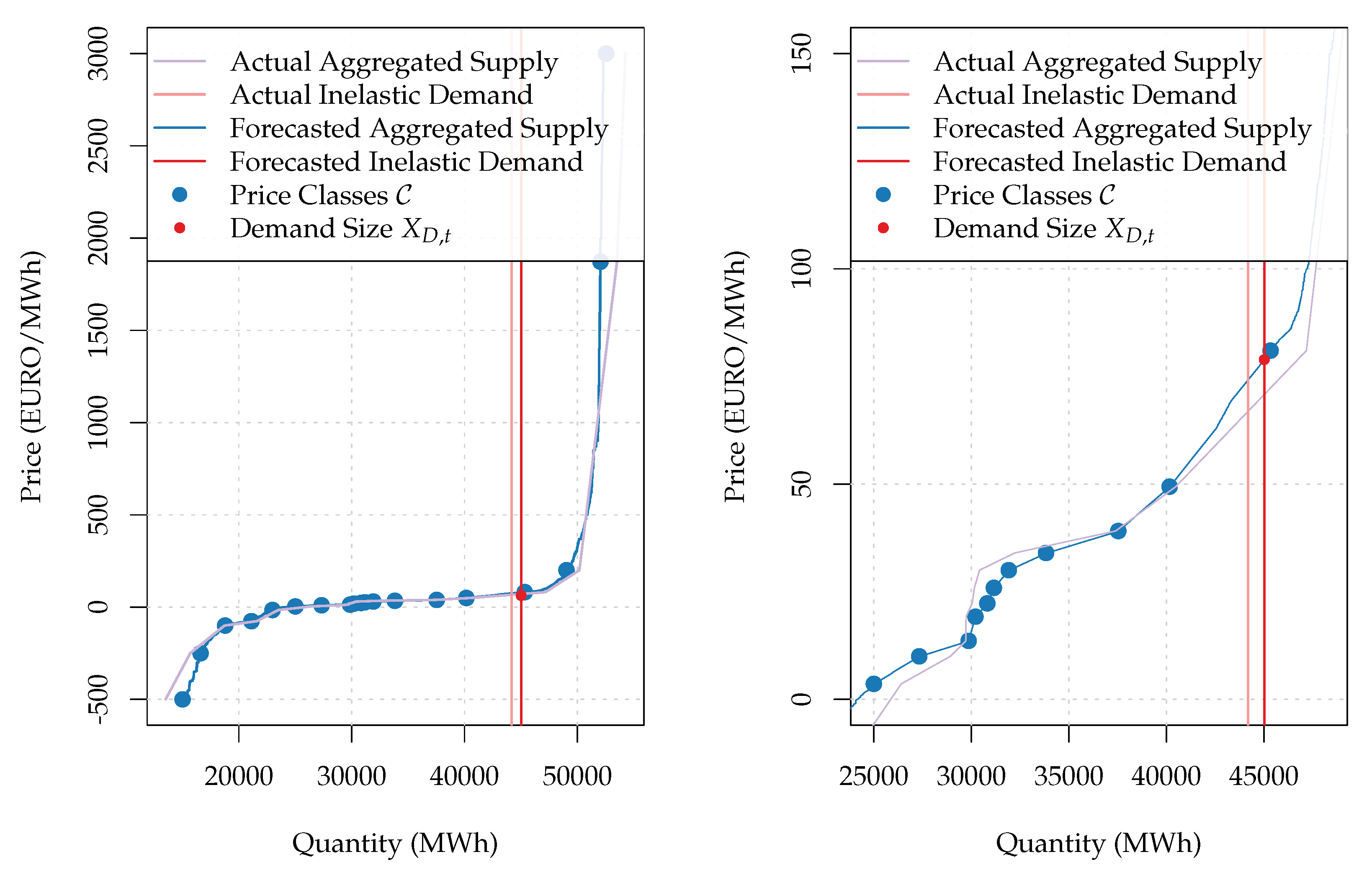
where $R\left(P\right)=1$ if a price occurs at least two times a day and $R\left(P\right)=0$ otherwise. Therefore, Equation (14) allows us to divide prices in price grid $\mathcal{P}$ into two categories. The first category includes prices at which market participants did not bid often (i.e., at least two times a day). The formula neglects these prices in the further calculation. On the contrary, the volume predicted within a given price class is distributed over the prices in the second category. The more often market participants placed their bids at a particular price, the greater the share of volume assigned to this price would be. As a result, the formula retains the non-linear structure and composition of the original supply curve. Please note that reconstructing the demand curve is not necessary since this curve is perfectly inelastic. Moreover, Figure 3 provides a graphical representation of the predicted vs. actual curves after the curve reconstruction was carried out. From the figure (especially between price classes $49.4$ and $81.0$), it can be seen clearly that price classes are connected with curved lines.

Finally, the forecast for the entire supply curve can be defined as:

$$\begin{array}{c}\hfill \begin{array}{c}\hfill {\check{S}}_{d,h}\left(P\right)=\sum _{\begin{array}{c}p\in {\check{\mathcal{P}}}_{d,h}\\ p\le P\end{array}}{\check{V}}_{d,h}\left(p\right)\mathrm{for}{\check{\mathcal{P}}}_{d,h}\end{array}\end{array}$$

(15)

where ${\check{\mathcal{P}}}_{d,h}=\{P\in \mathcal{P}|R\left(P\right)=1\}$. The price forecast is then an intersection between the above defined supply curve and the inelastic demand curve, i.e., ${\hat{P}}_{d,h}^{DA}={\check{S}}_{d,h}^{-1}\left({\hat{X}}_{D,d,h}\right)$

4. Results

To ease the notation, we will denote the original X-model by $xmo{d}^{original}$ and the modified X-model by $xmo{d}^{modified}$. Furthermore, the study was extended with a simple naive benchmark (as in, e.g., [40]) denoted by $naive$. The $naive$ model assumed that the value at $t+1$ was equal to the value at t. Moreover, following the findings of, e.g., [41] or [42], we considered an equally weighted mixture of the original and modified X-models. This mixture was referred to as a combined X-model and had the specification $xmo{d}_{d,h}^{combined}=0.5\ast P_{d,h}^{xmo{d}^{original}}+0.5\ast P_{d,h}^{xmo{d}^{modified}}$.

To test the performance of the models, a rolling window study was conducted. The size of the window was equal to 24 hours, and the out-of-sample period was the year 2017. The yearly comparison of the models is provided in

Table 2. Comparison of the yearly MAE and RMSE values of the naivebenchmark, the original X-model ([22]), the modified X-model with an inelastic demand curve, and an equally weighted mixture of the original and the modified X-models.

	MAE	RMSE	Average Execution Time (min)
$naive$	9.97	11.90	-
$xmo{d}^{original}$.	6.21	7.54	4.34
$xmo{d}^{modified}$.	5.12	6.45	1.40
$xmo{d}^{combined}$.	5.28	6.47	-

. Please note that our definitions of the MAE and RMSE values were analogous to those in the original paper or in, e.g., [43] and can be written as:

$$\begin{array}{c}\hfill \begin{array}{c}\hfill \mathrm{MAE}=\frac{1}{24D}\sum _{d=1}^D\sum _{d=h}^{24}|P_{d,h}^{DA}-{\hat{P}}_{d,h}^{DA}|\mathrm{and}\mathrm{RMSE}=\sqrt{\frac{1}{24D}\sum _{d=1}^D\sum _{h=1}^{24}{\left(P_{d,h}^{DA}-{\hat{P}}_{d,h}^{DA}\right)}^2}\end{array}\end{array}$$

(16)

where $P_{d,h}^{DA}$ is an actual day-ahead price, ${\hat{P}}_{d,h}^{DA}$ is a price forecast of a model, $D=364$, and h is an hour index. Thus, Table 2 shows explicitly that the $naive$ model had the worst performance in the comparison. Moreover, the modified X-model had the lowest MAE and RMSE values, even lower than those of the combined X-model. The better accuracy of the modified X-model can be explained by the model’s ability to better process outliers. This ability was especially important given that the X-model was designed to better capture price spikes. Besides the superior performance, the modified X-model delivered results ca. three times quicker than the original X-model. Naturally, the improvement was present because the amount of forecasted variables was almost twice smaller in the modified version of the X-model. Please note that execution speed may vary depending on the specification of the LASSO model and its parameters.

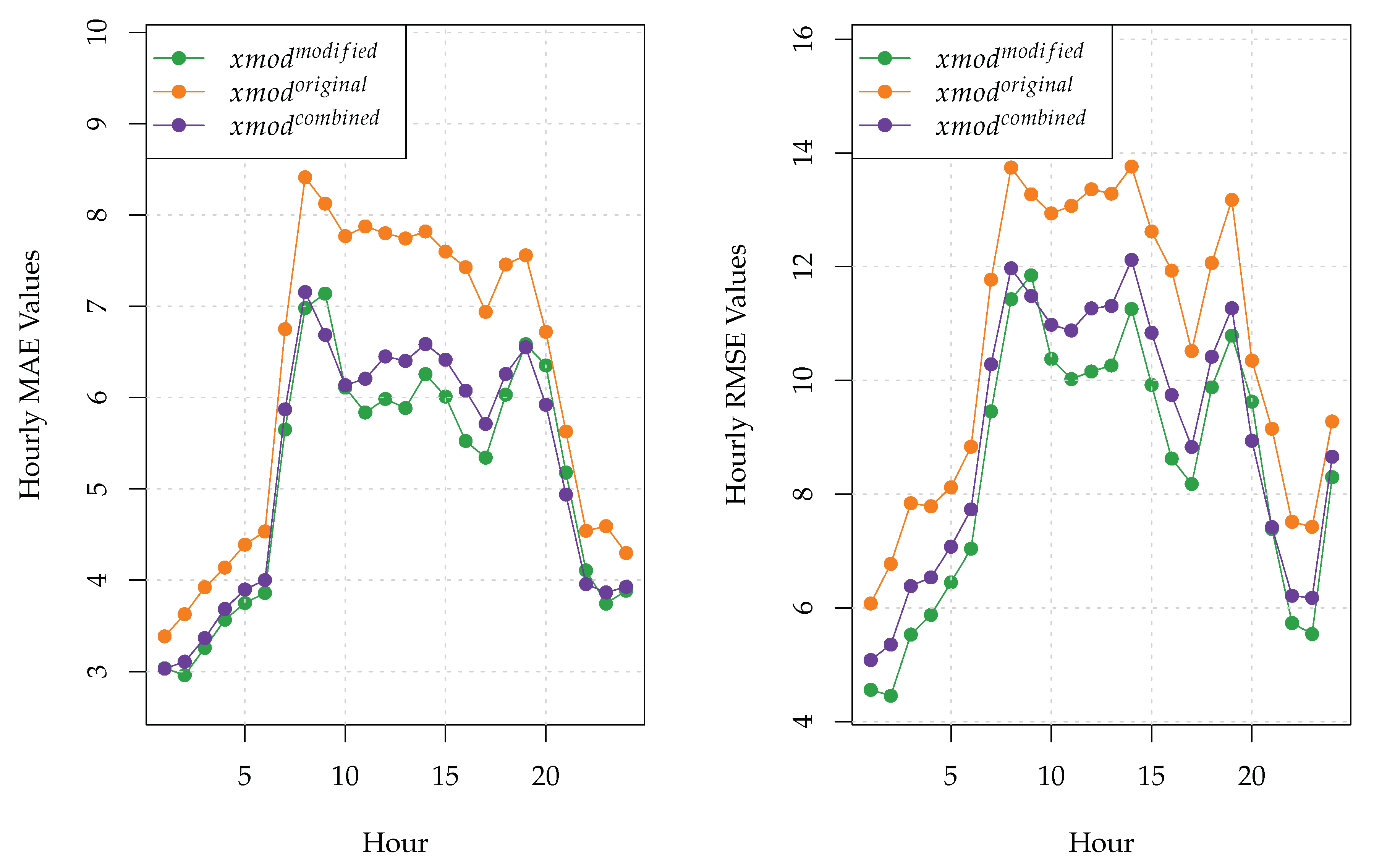
Furthermore, the MAE and RMSE values of the three X-models for each of the 24 h of the day are provided in Figure 4. The naive model was neglected in this figure due to the fact that its MAE and RMSE values were much higher than those of the X-models. As can be seen clearly from Figure 4, the modified X-model outperformed the original X-model during each hour of the day. In turn, the combined X-model had lower MAE values than the modified X-model during the hours 9, 20, 21, and 22. Moreover, the hourly RMSE values of the combined model were lower than those of the modified X-model only during the hours 9 and 20.

To determine best model, we used the DM-test formula as defined in [44]. The loss differential between models $\mathbb{A}$ and $\mathbb{B}$ for hour h was set to ${\delta }_{d,h,\mathbb{A},\mathbb{B}}=L_{d,h,\mathbb{A}}-L_{d,h,\mathbb{B}}$ where $L_{d,h}$ is the loss function of a model at hour h of day d. The respective loss functions of models $\mathbb{A}$ and $\mathbb{B}$ are $L_{\mathbb{A},d,h}={\left|{\hat{\epsilon }}_{\mathbb{A},d+i,h}\right|}^{\phi }$ and $L_{\mathbb{B},d,h}={\left|{\hat{\epsilon }}_{\mathbb{B},d+i,h}\right|}^{\phi },$ where $\phi =1,2$ to compare the models with respect to both absolute and quadratic errors. The t-statistic of the DM-test is defined as $t_{DM}={\overline{\delta }}_{h,\mathbb{A},\mathbb{B}}/{\sigma }_{\overline{\delta },h,\mathbb{A},\mathbb{B}}$ where ${\overline{\delta }}_{h,\mathbb{A},\mathbb{B}}=\frac{1}{D}{\sum }_{d=1}^D{\delta }_{d,h,\mathbb{A},\mathbb{B}}$ and ${\sigma }_{\overline{\delta },h,\mathbb{A}\mathbb{B}}$ denotes the standard deviation of ${\overline{\delta }}_{d,h,\mathbb{A},\mathbb{B}}$. The conducted DM-test proved that the modified X-model outperformed the original X-model over the course of the year 2017 (the corresponding p-value was equal to $2\times {10}^{-9}$). In fact, the results of hourly DM-tests indicated that the modified X-model was significantly better than the original X-model during each of the 24 hours of the day.

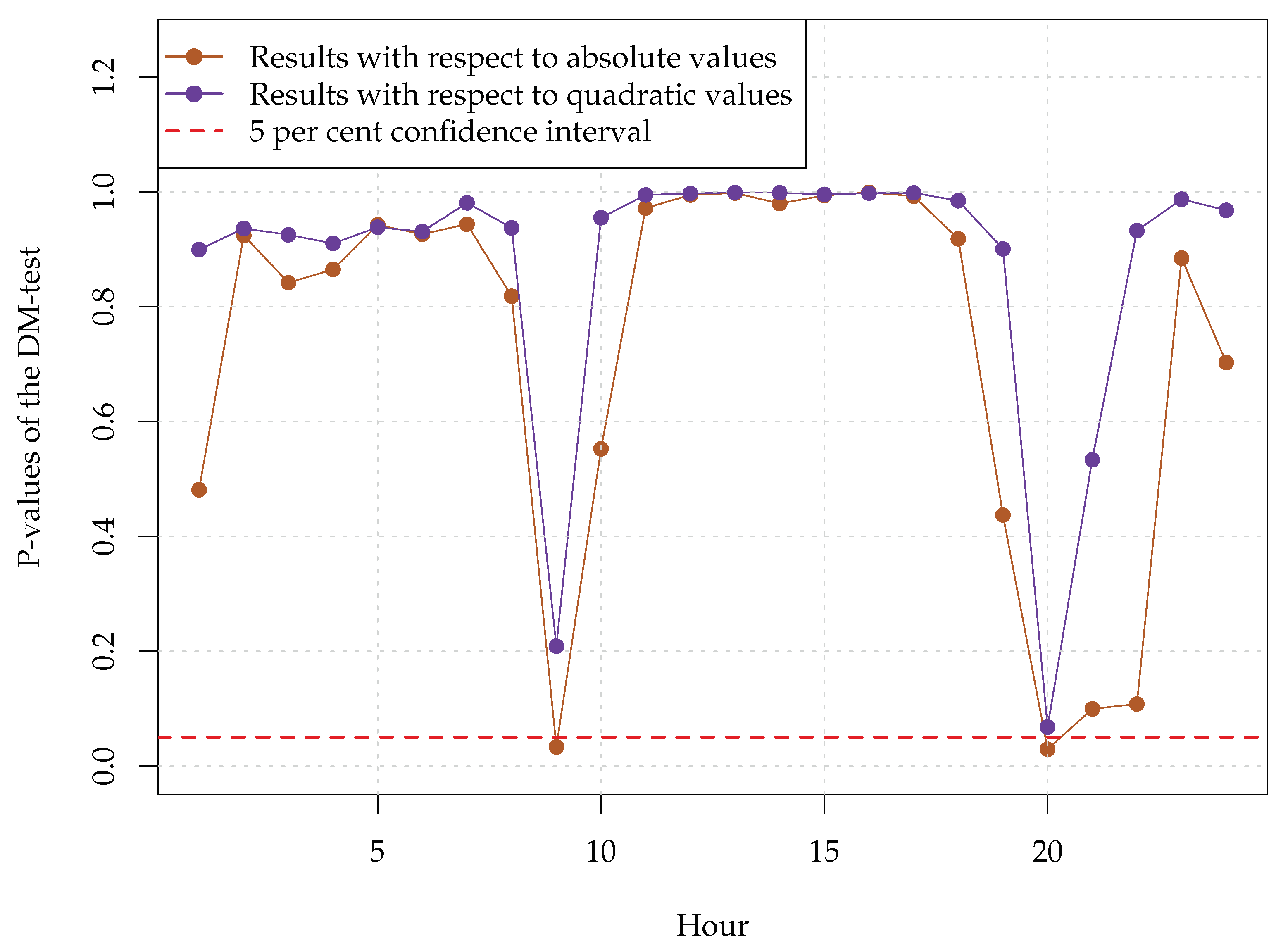
Furthermore, hourly DM-tests were conducted to compare the modified X-model $xmo{d}^{modified}$ with the combined X-model $xmo{d}^{combined}$. The obtained results are presented in Figure 5. The figure demonstrates that the latter model was significantly better than the former one during the hours 9 and 20 with respect to absolute errors. However, the combined X-model did not significantly outperform the modified X-model with respect to quadratic errors. A possible reason for this result is that the modified X-model was more robust towards outliers than the original X-model. Moreover, the fact that even the mixture of the two models failed to outperform the modified X-model significantly during most of the hours was yet another indication of the superiority of the modified X-model over the original one.

5. Conclusions

The goal of the present paper was to improve the original X-model derived by [22]. The improvement was based on the technique developed by [19]. This technique allowed us to transform the wholesale supply and demand curves into their analogues with a perfectly inelastic demand curve. We showed that modifying the X-model by means of this technique led to a significant improvement of the final results.

More specifically, the modified X-model was shown to work faster. A decrease of the execution speed was achieved because the demand curve after the transformation was represented by only one point instead of several price classes. Moreover, the modified version of the X-model was shown to be more robust towards outliers present in the initial auction curves’ data. Due to the way the auction curves were constructed by the electricity exchange, outliers were accumulated in the forecast for both the supply and demand curves in the original X-model. However, the cumulative effect was not present in the demand curve of the modified X-model. Therefore, the modified X-model yielded more accurate forecasts.

There are two possible ways to improve the X-model further. The first one is related to the issue of outliers. As was elaborated earlier, outliers are accumulated in the forecast for the entire supply curve in the modified X-model. This happens because the volumes in price classes $(2,\dots ,M_S)$ are added as increments to the volume $Y_{d,h}^{S,1}$ in the first price class. As a result, the entire segment $(c,\dots ,M_S)$ with $c>1$ of the supply curve is going to be shifted if there are outliers in any of price classes $(1,\dots ,c)$. To mitigate the problem, the following can be done. First, the last price class $M_S$ (i.e., the one at $P_{max}$) should be taken as the starting point for building the supply curve. In this case, volumes in price classes $(M_S-1,\dots ,1)$ are going to be incremented over the volume in price class $M_S$. Then, an average of the two supply curves with starting points $Y_{d,h}^{S,1}$ and $Y_{d,h}^{S,M_S}$, respectively, should be calculated. Hence, computing an average of two curves with opposite starting points allows the cumulative effect of outliers to be reduced. Analogously, a point in the middle of the supply curve can be taken as a starting point.

The second way concerns the selection of the price classes. The currently implemented method is rather simplistic and can be replaced with a more sophisticated technique. More specifically, applying an equidistant volume grid to an average supply curve does not provide any technical justification for selecting particular price classes. Instead, conventional clustering methods such as, e.g., the K-means algorithm or support vector machines can be used to select price classes.

References

- Weron, R. Electricity price forecasting: A review of the state-of-the-art with a look into the future. Int. J. Forecast. 2014, 30, 1030–1081. [Google Scholar] [CrossRef] [Green Version]
- Uniejewski, B.; Nowotarski, J.; Weron, R. Automated variable selection and shrinkage for day-ahead electricity price forecasting. Energies 2016, 9, 621. [Google Scholar] [CrossRef] [Green Version]
- Narajewski, M.; Ziel, F. Econometric modelling and forecasting of intraday electricity prices. J. Commod. Mark. 2019, 100107. [Google Scholar] [CrossRef] [Green Version]
- Tan, Z.; Zhang, J.; Wang, J.; Xu, J. Day-ahead electricity price forecasting using wavelet transform combined with ARIMA and GARCH models. Appl. Energy 2010, 87, 3606–3610. [Google Scholar] [CrossRef]
- Gianfreda, A.; Grossi, L. Forecasting Italian electricity zonal prices with exogenous variables. Energy Econ. 2012, 34, 2228–2239. [Google Scholar] [CrossRef] [Green Version]
- Liu, H.; Shi, J. Applying ARMA–GARCH approaches to forecasting short-term electricity prices. Energy Econ. 2013, 37, 152–166. [Google Scholar] [CrossRef]
- Cartea, A.; Figueroa, M.G. Pricing in electricity markets: a mean reverting jump diffusion model with seasonality. Appl. Math. Finance 2005, 12, 313–335. [Google Scholar] [CrossRef] [Green Version]
- Benth, F.E.; Kiesel, R.; Nazarova, A. A critical empirical study of three electricity spot price models. Energy Econ. 2012, 34, 1589–1616. [Google Scholar] [CrossRef]
- Ioannou, A.; Angus, A.; Brennan, F. Effect of electricity market price uncertainty modelling on the profitability assessment of offshore wind energy through an integrated lifecycle techno-economic model. J. Phys. Conf. Ser. IOP Publ. 2018, 1102, 012027. [Google Scholar] [CrossRef] [Green Version]
- Muniain, P.; Ziel, F. Probabilistic forecasting and simulation of electricity prices. arXiv 2018, arXiv:1810.08418. [Google Scholar]
- Karakatsani, N.V.; Bunn, D.W. Forecasting electricity prices: The impact of fundamentals and time-varying coefficients. Int. J. Forecast. 2008, 24, 764–785. [Google Scholar] [CrossRef]
- Weron, R. Heavy-tails and regime-switching in electricity prices. Math. Method Oper. Res. 2009, 69, 457–473. [Google Scholar] [CrossRef] [Green Version]
- Bordignon, S.; Bunn, D.W.; Lisi, F.; Nan, F. Combining day-ahead forecasts for British electricity prices. Energy Econ. 2013, 35, 88–103. [Google Scholar] [CrossRef] [Green Version]
- Eichler, M.; Türk, D. Fitting semiparametric Markov regime-switching models to electricity spot prices. Energy Econ. 2013, 36, 614–624. [Google Scholar] [CrossRef] [Green Version]
- Janczura, J.; Weron, R. Efficient estimation of Markov regime-switching models: An application to electricity spot prices. AStA Adv. Stat. Anal. 2012, 96, 385–407. [Google Scholar] [CrossRef] [Green Version]
- Barlow, M.T. A diffusion model for electricity prices. Math. Finance 2002, 12, 287–298. [Google Scholar] [CrossRef]
- Buzoianu, M.; Brockwell, A.; Seppi, D. A dynamic supply-demand model for electricity prices. Technical report, Carnegie Mellon University, 2012. Available online: https://kilthub.cmu.edu/articles/A_Dynamic_Supply-Demand_Model_for_Electricity_Prices/6586331 (accessed on 10 December 2019).
- Aneiros, G.; Vilar, J.M.; Cao, R.; San Roque, A.M. Functional prediction for the residual demand in electricity spot markets. IEEE Trans. Power Syst. 2013, 28, 4201–4208. [Google Scholar] [CrossRef]
- Coulon, M.; Jacobsson, C.; Ströjby, J. Hourly resolution forward curves for power: Statistical modeling meets market fundamentals. In Energy Pricing Models: Recent Advances, Methods, and Tools; Palgrave Macmillan: London, UK, 2014. [Google Scholar]
- Carmona, R.; Coulon, M.; Schwarz, D. Electricity price modeling and asset valuation: a multi-fuel structural approach. Math. Financ. Econ. 2013, 7, 167–202. [Google Scholar] [CrossRef] [Green Version]
- Howison, S.; Coulon, M. Stochastic behaviour of the electricity bid stack: from fundamental drivers to power prices. J. Energy Mark. 2009, 2, 29–69. [Google Scholar]
- Ziel, F.; Steinert, R. Electricity price forecasting using sale and purchase curves: The X-Model. Energy Econ. 2016, 59, 435–454. [Google Scholar] [CrossRef] [Green Version]
- Shah, I.; Lisi, F. Forecasting of electricity price through a functional prediction of sale and purchase curves. J. Forecast. 2020, 39, 242–259. [Google Scholar] [CrossRef]
- Canale, A.; Vantini, S. Constrained functional time series: Applications to the Italian gas market. Int. J. Forecast. 2016, 32, 1340–1351. [Google Scholar] [CrossRef]
- Dillig, M.; Jung, M.; Karl, J. The impact of renewables on electricity prices in Germany–An estimation based on historic spot prices in the years 2011–2013. Renew. Sustain. Energy Rev. 2016, 57, 7–15. [Google Scholar] [CrossRef]
- Kulakov, S.; Ziel, F. The impact of renewable energy forecasts on intraday electricity prices. arXiv 2019, arXiv:1903.09641. [Google Scholar]
- Kulakov, S.; Ziel, F. Determining the Demand Elasticity in a Wholesale Electricity Market. arXiv 2019, arXiv:1903.11383. [Google Scholar]
- Knaut, A.; Paulus, S. When are consumers responding to electricity prices? An hourly pattern of demand elasticity. EWI Working Papers. 2016. Available online: https://ideas.repec.org/p/ris/ewikln/2016_007.html (accessed on 10 December 2019).
- Viehmann, J. State of the german short-term power market. Zeitschrift für Energiewirtschaft 2017, 41, 87–103. [Google Scholar] [CrossRef]
- Kiesel, R.; Paraschiv, F. Econometric analysis of 15-minute intraday electricity prices. Energy Econ. 2017, 64, 77–90. [Google Scholar] [CrossRef] [Green Version]
- EPEX. Day Ahead Prices and Volumes Data. 2019. Available online: https://www.epexspot.com/de/marktdaten/dayaheadauktion (accessed on 30 June 2019).
- EPEX. Day Ahead Auction Curves Data. 2019. Restrictions on the Data Are Applied, For More See. Available online: https://www.epexspot.com/de/marktdaten/dayaheadauktion/preiskurve/auction-aggregated-curve/2019-07-30/DE/00 (accessed on 30 June 2019).
- ENTSO-E. Wind, Solar and Load Actual and Forecasted Data. 2019. Restrictions on the Data Are Applied, For More See. Available online: https://www.entsoe.eu/data/power-stats/ (accessed on 30 June 2019).
- Weron, R. Modeling and Forecasting Electricity Loads and Prices: A Statistical Approach; John Wiley & Sons: Hoboken, NJ, USA, 2007; Volume 403. [Google Scholar]
- Weron, R.; Misiorek, A. Forecasting spot electricity prices: A comparison of parametric and semiparametric time series models. Int. J. Forecast. 2008, 24, 744–763. [Google Scholar] [CrossRef] [Green Version]
- Ziel, F. Forecasting electricity spot prices using lasso: On capturing the autoregressive intraday structure. IEEE Trans. Power Syst. 2016, 31, 4977–4987. [Google Scholar] [CrossRef] [Green Version]
- Tibshirani, R. Regression shrinkage and selection via the lasso. J. R. Stat. Soc. Ser. B (Methodol.) 1996, 58, 267–288. [Google Scholar] [CrossRef]
- Schwarz, G. Estimating the dimension of a model. Ann. Stat. 1978, 6, 461–464. [Google Scholar] [CrossRef]
- Friedman, J.; Hastie, T.; Tibshirani, R. Regularization paths for generalized linear models via coordinate descent. J. Stat. Softw. 2010, 33, 1. [Google Scholar] [CrossRef] [Green Version]
- Ziel, F.; Steinert, R.; Husmann, S. Forecasting day ahead electricity spot prices: The impact of the EXAA to other European electricity markets. Energy Econ. 2015, 51, 430–444. [Google Scholar] [CrossRef] [Green Version]
- Granger, C.W.; Ramanathan, R. Improved methods of combining forecasts. J. Forecast. 1984, 3, 197–204. [Google Scholar] [CrossRef]
- Nowotarski, J.; Liu, B.; Weron, R.; Hong, T. Improving short term load forecast accuracy via combining sister forecasts. Energy 2016, 98, 40–49. [Google Scholar] [CrossRef]
- Uniejewski, B.; Weron, R.; Ziel, F. Variance stabilizing transformations for electricity spot price forecasting. IEEE Trans. Power Syst. 2017, 33, 2219–2229. [Google Scholar] [CrossRef] [Green Version]
- Diebold, F.X. Comparing predictive accuracy, twenty years later: A personal perspective on the use and abuse of Diebold–Mariano tests. J. Bus. Econ. Stat. 2015, 33, 1–8. [Google Scholar] [CrossRef] [Green Version]
Sample Availability: Samples of the compounds as well as the source code are available from the authors for review purposes. |
Figure 1.
A wholesale market equilibrium in the EPEXSPOTSEon 2017-02-01 at 00:00:00 (left plot) vs. its manipulated form with an inelastic demand curve (right plot).
Figure 2.
A wholesale market equilibrium in the EPEX SPOT SE on 2017-02-01 at 00:00:00 with transformed auction curves and highlighted price classes. The left-hand side of the figure shows the entire auction curves recorded at the time point. The right-hand side of the figure plots the same curves, but focuses on the equilibrium between them.
Figure 3.
Market equilibrium forecast on 2017-02-01 at 10-00-00. The left-hand side of the figure shows the entire auction curves recorded at the time point. The right-hand side of the figure plots the same curves, but focuses on the equilibrium between them.
Figure 4.
Hourly MAE (left-hand side) and RMSE (right-hand side) values of the modified X-model (), the original X-model (), and the combined X-model ().
Figure 5.
p-values for each hour of the day of the comparison of the models vs. according to the DM-test. As can be seen from the figure, the modified X-model outperformed the combined X-model during most hours of the day.