Performance Comparison between Deep Learning and Optical Flow-Based Techniques for Nowcast Precipitation from Radar Images


CRS4, Center for Advanced Studies, Research and Development in Sardinia, loc. Piscina Manna ed. 1, 09050 Pula, Italy
*
Author to whom correspondence should be addressed.
Forecasting 2020, 2(2), 194-210; https://0-doi-org.brum.beds.ac.uk/10.3390/forecast2020011
Submission received: 26 May 2020
/
Revised: 13 June 2020
/
Accepted: 22 June 2020
/
Published: 24 June 2020
(This article belongs to the Special Issue Feature Papers of Forecasting)
Abstract
:In this article, a nowcasting technique for meteorological radar images based on a generative neural network is presented. This technique’s performance is compared with state-of-the-art optical flow procedures. Both methods have been validated using a public domain data set of radar images, covering an area of about 104 km2 over Japan, and a period of five years with a sampling frequency of five minutes. The performance of the neural network, trained with three of the five years of data, forecasts with a time horizon of up to one hour, evaluated over one year of the data, proved to be significantly better than those obtained with the techniques currently in use.
1. Introduction
Forecasting precipitation at very high resolutions in space and time, particularly with the aim of providing the boundary conditions for hydrological models and estimating the associated risk, is one of the most difficult challenges in meteorology [1]. In short, the problem is to predict the field of precipitation on grids of 1 km or less and for horizons of less than a few hours (nowcast) [2]. Due to the high spatial resolutions required, methods based on meteorological models are not effective, because they are too onerous computationally and the time to perform a simulation is usually excessively too long for operational purposes. They also depend, in a critical way, on the initial conditions as the level of uncertainty is too high and it is difficult to assimilate locally recorded data [3,4]. Even if these difficulties were overcome, a fundamental difficulty would remain, the gap between the spatial scales provided by the meteorological models and those useful to hydrologists for operational purposes. To overcome this difficulty and quantify the uncertainty involved, probabilistic approaches were proposed [5].
In contrast, simplified approaches based on image processing and related data extrapolation, based on radar reflectivity or remote sensing data, have proven to be more effective. For example in [6], an application in Mediterranean basins of a semi-distributed hydrological model using rainfall estimated by radar was discussed, and in a more recent paper an application with a coupled soil and groundwater model was discussed [7]. A study discussing the propagation of the uncertainty in weather radar estimates of rainfall through hydrological models can be found in [8]. This approach showed to be even more promising by using new methodologies based on recent advances in deep learning techniques [9].
The simplest techniques for nowcasting on meteorological radar data consist of two phases, tracking and extrapolation, i.e., first the velocity field is estimated, typically with image comparison techniques called Optical Flow (OF), this field is then used to extrapolate a prediction of radar images through semi-Lagrangian schemes, or interpolation procedures [10]. This procedure estimates the precipitation as seen by the radar, assuming that the rate of advection evaluated by comparing a sequence of two or more consecutive images stays constant with no terms of sink or source altering the intensity of the field in the chosen forecast range. Unfortunately these two assumptions, given the high space-temporal variability of the precipitation, most never occur, and this is all the more true the longer the forecast time horizon is. For this reason, a forecast procedure based on optical flow has a limited validity with lead times of the order of the hour. Despite this, there are several nowcasting procedures for radar images and related by-products based on OF, operational in meteorological centers, that are able to provide predictions with appreciable skills with a time horizon of up to three hours [11,12], when used with additional information from numerical model’s data, and real-time precipitation measurements. For this reason, the topic, although widely investigated, is still of interest for research [13]. This work will focus on the analysis of nowcast methods based only on radar data. The intent is to assess the degree of the predictive potential of the data itself and with the idea that this can add value even when operating in conjunction to additional information.
The first nowcasting methods based on OF [14] foresaw the evolution of the image from one instant to the next by means of a rigid translation, with an advection field determined by the criteria of maximum correlation between two or more images, immediately preceding the time of emission of the forecast. In the TREC method, the advection field is not constant but is evaluated by comparing boxes of pixels of equal size between two successive radar images, and identifying similar boxes through cross correlation. An advection vector connects the centers of two similar boxes. Repeating the process on boxes of optimal size distributed on the image, it is possible to determine a non constant field of advection that is then used for the extrapolation of the precipitation field [15]. Over the years these methods have been refined, providing the possibility to advect separately the features defined as “interesting” within the images, such as the position of the precipitating centers, or the maximum gradient points, as in the method described in Shi-Tomasi [16]. Then the possibility of deformation of the advected pattern was added, applying for example an affine transformation [17]. All these methods and several other variants have the conceptual limitation of being deterministic, not taking into account the high uncertainty inherent in this overly simplistic approach. The so-called SPROG [18] approach takes into account the diverse predictability of the precipitation at different scale. It decomposes the logarithmic transformation of the initial field into a multiplicative cascade of decreasing spatial scale fields, and advects each of them separately, keeping the coherence with the pre-forecast period. Finally, the field at each forecast deadline is calculated as the antilogarithm of the product of the fields at the individual scales. More details of this and other techniques used as benchmarks will be provided in the following section.
More recently, the potential offered by the highly non-linear approach of neural networks has been investigated. These techniques use a large amount of past data to “learn” and devise a predictive model. The first studies that have started this line of research for forecasting precipitation from radar images have been introduced by the Hong-Kong Meteorological Observatory Group [19,20]. In a work published in 2015 [19], the authors introduced the ConvLSTM model and demonstrated that it outperforms the OF-based operating model, called SWIRLS (Short term forecast of Intense Rain Localized Systems), for forecasting horizons of up to two hours. In a follow up [20], the same authors have introduced the TrajGRU model, which uses the same convolutional and recursive deep networks as the previous one, but where a location feature for radar image processing is introduced, improving the performance of both SWIRLS and convLSTM models. Recently a variant of PredNet architecture has been proposed in [21] while in [22] a completely convolutional deep neural network is used, investigating in particular the importance of data pre-processing, network structure and loss function.
With the aim of investigating and comparing the predictive potential of different approaches and, in order to find methods that can offer room for improvement, this work proposes and evaluates the performance of a PredNet deep neural network [23]. The architecture is borrowed from computer vision for short-term video prediction, where it represents one of the state of the art approaches.
Compared to [21], where a similar network was used, this version has a modified loss function for training phase that tries to maximize the predictive performance of the architecture. A quantitative and qualitative comparison of the results obtained with the PredNet versus the reference OF methods is presented here that will highlight not only the different performance but also the distinct characteristics of the forecast obtained, and their limits.
The rest of the paper is organized as follows: Section 2 illustrates the methodologies used as benchmarks, Section 3 presents the modified neural network used in this analysis, Section 4 describes the data used for the numerical comparison while results are discussed in Section 5. Section 6 hosts the conclusions and a discussion of potential future developments.
2. Benchmark Nowcast Techniques
The methodologies used as benchmarks to assess the performance of the approach proposed in this paper are those implemented in two public domain libraries called rainymotion [10] and pysteps [24].
The rainymotion library, built on opencv [25], implements four different nowcasting methods called Dense, Dense Rotation, SparseSD and Sparse. The Dense and Dense Rotation methods are based on standard Optical Flow estimation techniques. The Sparse and SparseSD methods, instead of tracking the displacement of all pixels in the image, first detect a chosen number of “good features to track” [16], typically the boundaries of moving objects with respect to the constant background, and trace their most likely displacement with optical flow techniques [14]. Next, they calculate, and apply, the affine transformation that maps the “interesting” features from one frame to the following [17] and eventually fill the final image by interpolation [26]. The Sparse method uses a sequence of images of variable length (in our case 12) preceding the instant of the nowcast, in order to trace the “interesting” characteristics of the field, while SparseSD uses only the last two images. Since, in all the tests we carried out, the Sparse (SP henceforth) and Dense Rotation (DR henceforth) methods have proven to perform better than the corresponding SparseSD and Dense methods, the results presented below will be only related to SP and DR.
Pysteps [24] is also a public domain library, managed and developed by a large community, which besides being an operational tool for nowcasting, is used as a development and study platform for the implementation of new techniques. For the estimation of the field of advection, pysteps implements three methodologies: a local type based on the classic Lucas-Kanade (LK) technique [14,27], a global variational type (VET) [28,29] and a spectral type (DARTS) [30]. Extrapolation by advection is done with a semi-lagrangian scheme backward in time [29]. The most sophisticated technique of the pysteps library, used here as a benchmark, is called STEPS, takes into account the different predictability of the precipitation phenomena at different scales. In practice, using an approach called SPROG [18], after a logarithmic transformation, a decomposition of the initial field into a multiplicative cascade of fields with decreasing spatial scales is performed and each of these spatial fields is advanced with an advection obtained consistently during the period before the nowcast. The decomposition of the field at different scales can be achieved using techniques of varying degrees of complexity, such as Discrete Cosine Transform or wavelet. In this case an FFT was used in which the different portions of the spectrum are weighed by Gaussian functions [31] and then, by inverse FFT, brought back into the spatial domain. The additional uncertainty due to the fact that, during the period of the forecast validity there may be growth, decay, creation and/or definitive disappearance of the precipitating cells, alongside the uncertainties linked to different spatial scales, were taken into account trough a stochastic noise built on the space and time variability, observed in the period preceding the emission, added to each partial field. For the implementation details please refer to [24] and the references therein. This approach makes it possible to obtain not a single deterministic forecast, but a set of equally probable forecasts (ensemble) and therefore also to quantify its space-time uncertainty. In this work, we limited ourselves to study the performance of deterministic forecasts, deliberately avoiding to discuss aspects related to space-time uncertainty, aspects that emerge from the discussion at the end of Section 5. To allow the comparison also with the other methodologies we will use the deterministic forecast obtained averaging all the STEP members and we will indicate this estimate with ST hereafter.
3. Proposed Nowcast Technique
The nowcasting problem can be tackled with artificial intelligence techniques exploiting the recent results of neural network approaches in the fields of computer vision and natural language processing. As a matter of fact, radar imagery nowcasting can be thought as a supervised learning problem, where the parameters of a neural network are modified to minimize an objective function that depends on the differences between the estimated precipitation image and the real field. Among the various network architectures proposed in computer vision and, in some cases, also already applied to the problem of meteorological nowcasting, we opted for the PredNet model, developed in computer vision for the forecasting of future frames in a video sequence. A key insight of this and other deep neural network methods is that, in order to be able to predict how the visual scenery will change over time, an agent must have at least some implicit structural model of the object represented by the sequence of images and the possible transformations that these objects may undergo. In the case of precipitation nowcasting this translates into the need for the network to assimilate a representation of the movement of the clouds and the development of related precipitation. In the proposed architecture, this translates into the ability to interpret the cloud movements considering the advective part of the phenomena, and also predict variations in intensity, linked for example to the orography of the domain.
The PredNet architecture [23] continuously strives to predict the appearance of future video frames, using a deep and recursive convolutional network with connections from large scale to small scale (top-down) and vice versa. The approach exploits the experience of similar models based on recursive and convolutional networks for the prediction of successive video frames, but draws particular inspiration from the concept of “predictive coding” in neuroscience literature, which assumes that the brain continuously makes predictions by anticipating incoming sensory stimuli. The top-down connections of the PredNet network transmit these forecasts, gradually increasing the details, compared with real observations, to generate an error signal. This is then propagated back to coarser scales (bottom-up) across the network, ultimately leading to a forecast update.
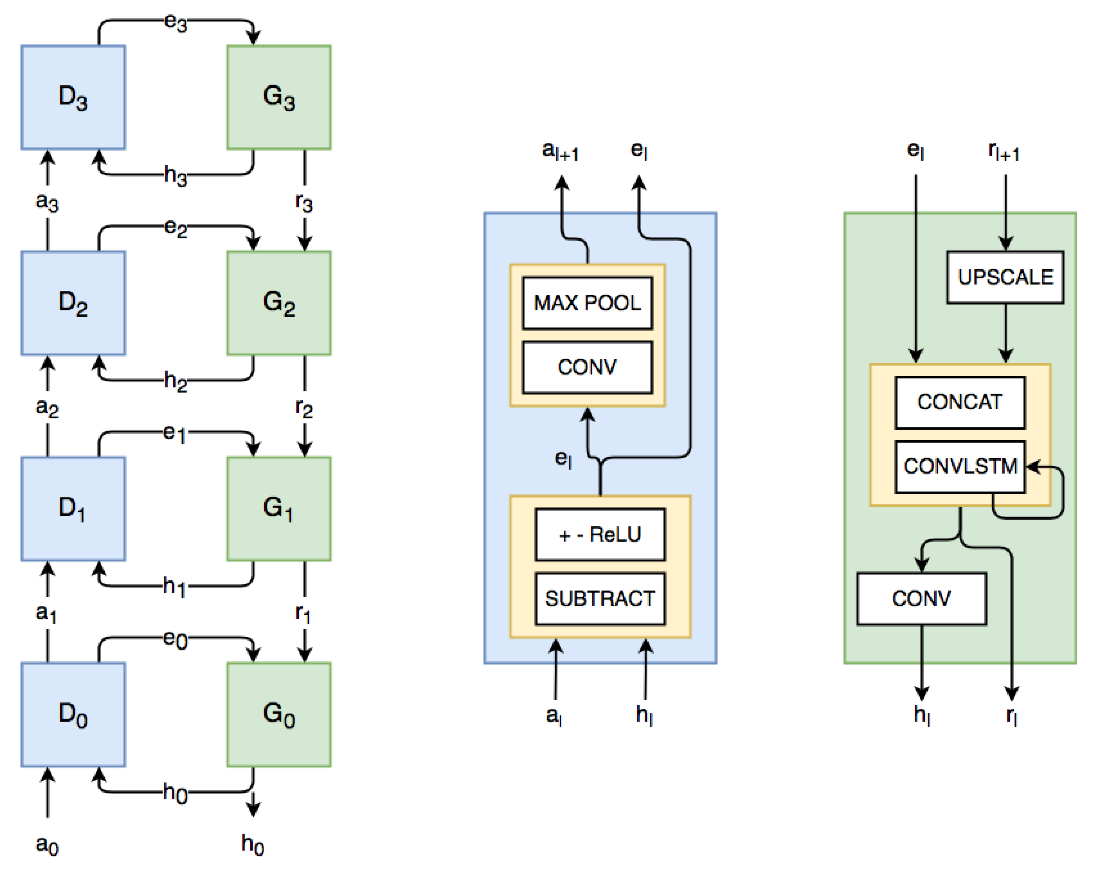
The PredNet architecture used is shown schematically in Figure 1 and consists of a ladder structure with a descending branch that generates the prediction of the precipitation field image at progressively more detailed scales, and an ascending branch where the prediction is compared with the real data.
The generative block receives as input a representation of the state coming from the upper block , performs an upscaling (with factor 2) and concatenates the image thus obtained with the representation of the error for that scale, calculated at the previous iteration and stored in memory. This data is passed to a recurrent Long Short-Term Memory cell with convolutional filters [19], which in turn retains a memory of its own state. The result of processing is the state at the l layer, , where this image is further processed by a convolutional layer to get a representation of the precipitation .
The discriminant block receives as input the precipitation forecast for the scale under examination, and the representation of the real precipitation field at the same scale . From the comparison of the two images an error image is generated. This is stored in memory as the input of the generative block at the next iteration of the model, and is further processed by convolution and pooling, generating a representation of the precipitation of lower detail, passed then to the upper discriminative block.
Table 1 shows the tensor sizes used in the model. The convolution filters have a kernel size of 3 with a padding of 1. The hidden state for the LSTM network has a size equal to the tensors .
The model, as already said, provides more accurate results as new inputs are provided. The procedure presented here uses the images of the precipitation for the hour before the lead time, then the model is further iterated for the next hour’s forecast times, replacing the real image of precipitation with the one that the model estimated . With a time sampling of 5 min, 12 images for the first hour are provided and 24 images for the reconstruction of the first hour of precipitation and the estimates (without radar input) for the following hour are obtained by model iteration.
More details about the architecture can be found in Lotter, Kreiman and Cox [23]. This work is focused on forecasting the next frame in a video sequence, and it shows how the architecture is able to generate increasingly accurate forecasts as new frames are input, demonstrating to be able to refine forecasts and learn from mistakes made during the process. The training is performed with a Gradient Descent procedure in which the network parameters are changed to minimize errors at the different levels of image representation with a loss function based on Mean Absolute Error. The results obtained in [23] show that in case of real video sequence the best results are achieved with the minimization of only, i.e., the MAE between the calculated and the actual image.
Based on those results here the loss function is released from the representation of the internal error in the network and the minimization of the Mean Squared Error between the image of the estimated and the actual precipitation is used.
Since the forecast is extended beyond the next frame, the loss function used in the training phase is realized as the Mean Squared Error of the 24 images generated by the network compared to the real precipitation images:
where MSE is an operator that returns the Mean Squared Error between the actual radar image and the one estimated by the model; the sum is extended both to the 12 steps used for learning the current weather situation and to the 12 steps of the forecast, in order to train the network to “optimally” reconstruct both the radar images used as initial conditions and the predicted ones. Other experiments have also been carried out, using for example the MAE as loss function, obtaining, in the verification, an improvement limited to the specific metric (i.e., the MAE) but a more marked worsening for all the other metrics considered (i.e.,: RMSE, r and ETS). By using both MSE and MAE we verified that the training of a specific network for each forecast horizon did not produce an improvement in performance. Furthermore, tests were conducted using both the normalized rain intensity and a logarithmic transformation to feed NN. The best results were obtained using directly the color indexes of the image, and only after the predictive phase the rain rate transformation function described in Table 2. The weights of the neural network are optimized using a Gradient Descent procedure with Adam optimizer. Having data from 2013 to 2017 we used the images of the first 3 years for training, the images of 2016 for validation while the tests were conducted on the radar images of 2017. The neural network model and training procedures are implemented in python [32] using the PyTorch library [33] and are available in open source (https://github.com/lmssdd/RadarNowcast), the calculation was run on NVIDIA Tesla K80 GPU with 12GB of onboard RAM. The model will be referenced hereafter as NN.
4. Data
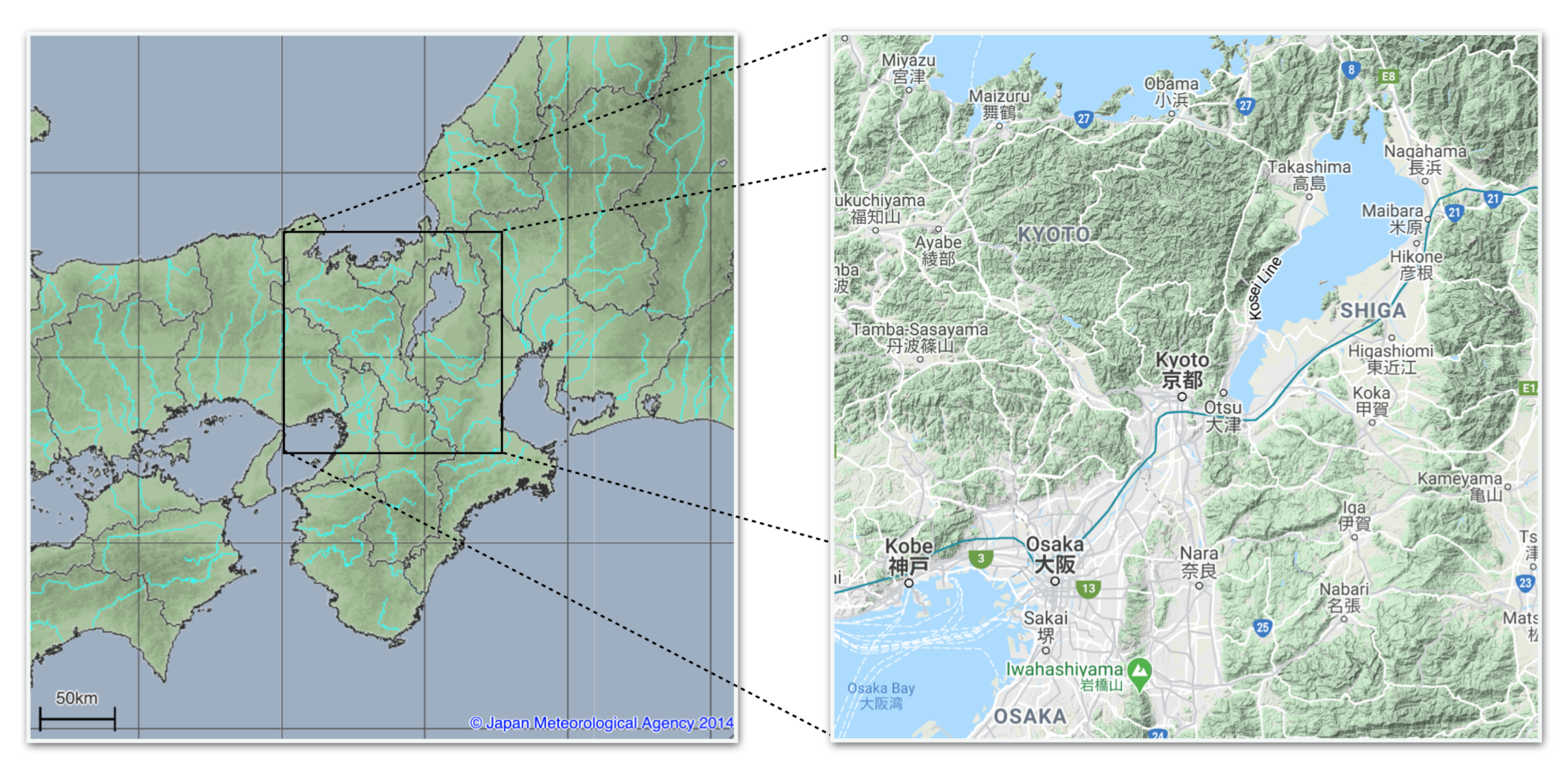
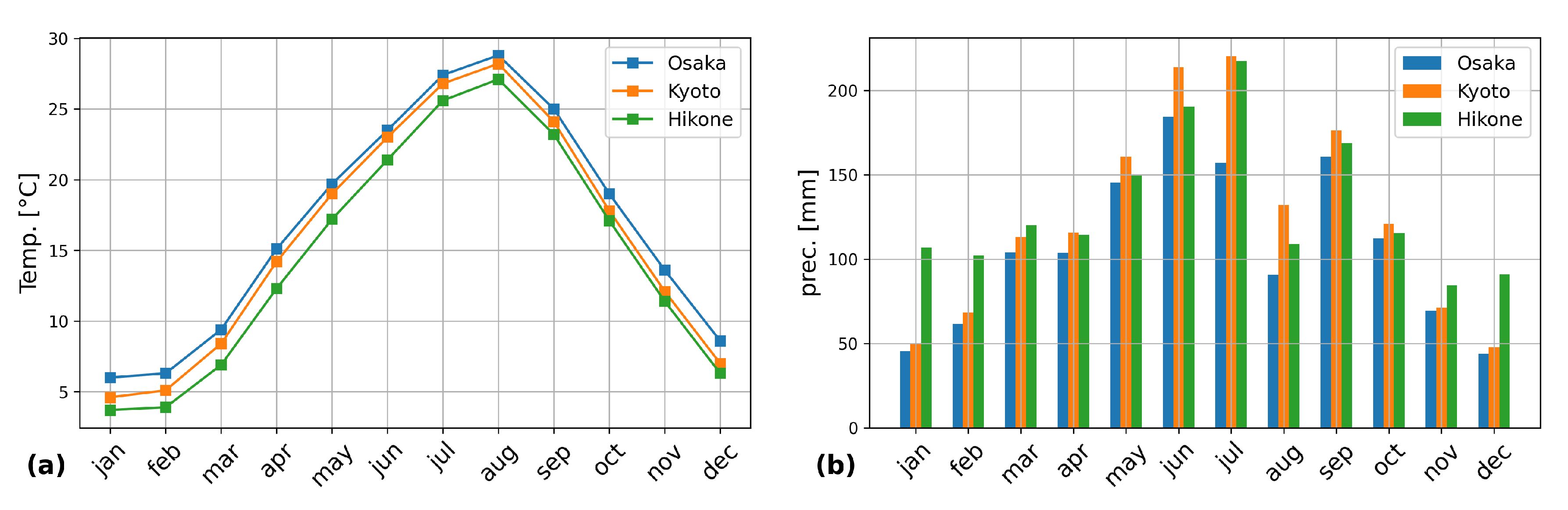
The data used in this application come from a meteorological radar located in the region between Osaka and Kyoto. These public domain data, already used in [21], have been collected from an online archive available on Yahoo (https://developer.yahoo.co.jp/webapi/map/openlocalplatform/v1/js/) and span five consecutive years from 2013 to 2017. Their spatial resolution is equal to 1 km2, the temporal frequency is 5’, the domain covers an area of about 104 km2 as shown in Figure 2 (https://www.jma.go.jp/en/highresorad/ and https://www.google.com/maps). The climate of the area is classified as hot-temperate, precipitation is intense (cumulative annual 1730 mm) and particularly heavy during the summer season as shown for 3 meteorological stations in Figure 3 (http://ds.data.jma.go.jp/gmd/tcc/tcc/products/climate/).
The dimension of the images obtained through the API is 1000 × 1000 pixels. After a crop necessary to remove text characters in the image, since the actual resolution of the radar is lower, a down-sampling of the image is performed, finally generating a 96 × 96 matrix. The data represent the precipitation intensity per pixel in a palette of 15 false colors. It is thus possible to map the colors as a progressive index of rain intensity with a range from 0 to 14 as reported in the Table 2.
The array containing the color index is normalized to a maximum unitary value to be processed in the neural network, and it is mapped back to rain intensity values during the post-processing. The use of precipitation intensity, or its elaboration using a logarithmic transform, has proven to be less effective than direct processing of the color scale index. The data has also been filtered by eliminating all weather events where the radar images were incomplete (i.e., either totally or partially missing).
All other methods have been applied to the logarithm transform of the rain rate estimates and only on rainy events, defined as those with at least 5% of the domain with precipitation rate greater or equal to 1 mm/h. The comparison between the different methodologies is limited to 2017, to maximize the use of previous years for the neural network training and favour a direct comparison with the results of optical flow methodologies that, instead, do not require training.
In the operational phase, all methods applied need to process a different number of the most recent steps of the radar images. The Table 3 lists the number of time steps needed for processing and the number of forecast steps obtained by each procedure. The NN and SP methodologies need, as initial conditions, several steps equal to the number of forecast occurrences, while all others can work with only two time steps except ST that needs three steps as initial condition.
5. Results
The performance of NN, ST, SP, DR, LK nowcasting techniques described in the Section 2 and Section 3, were assessed for 2017. The 2013, 2014 and 2015 data were used for training, the data of year 2016 were used for validation of the NN method. The performance indicators were evaluated against the precipitation value, at forecast verification time as estimated by the radar itself. Therefore, although expressed in mm/h, they do not represent in any way an estimate of the predicted precipitation forecast error. As a matter of fact, they gauge the error of the radar measures once transformed into mm/h. The indicators used are: the root mean square error (RMSE), the mean absolute error (MAE), the Pearson correlation coefficient (r), and the equitable threat score (ETS) for precipitation exceeding 0, 1, 2, 4 mm/h respectively.
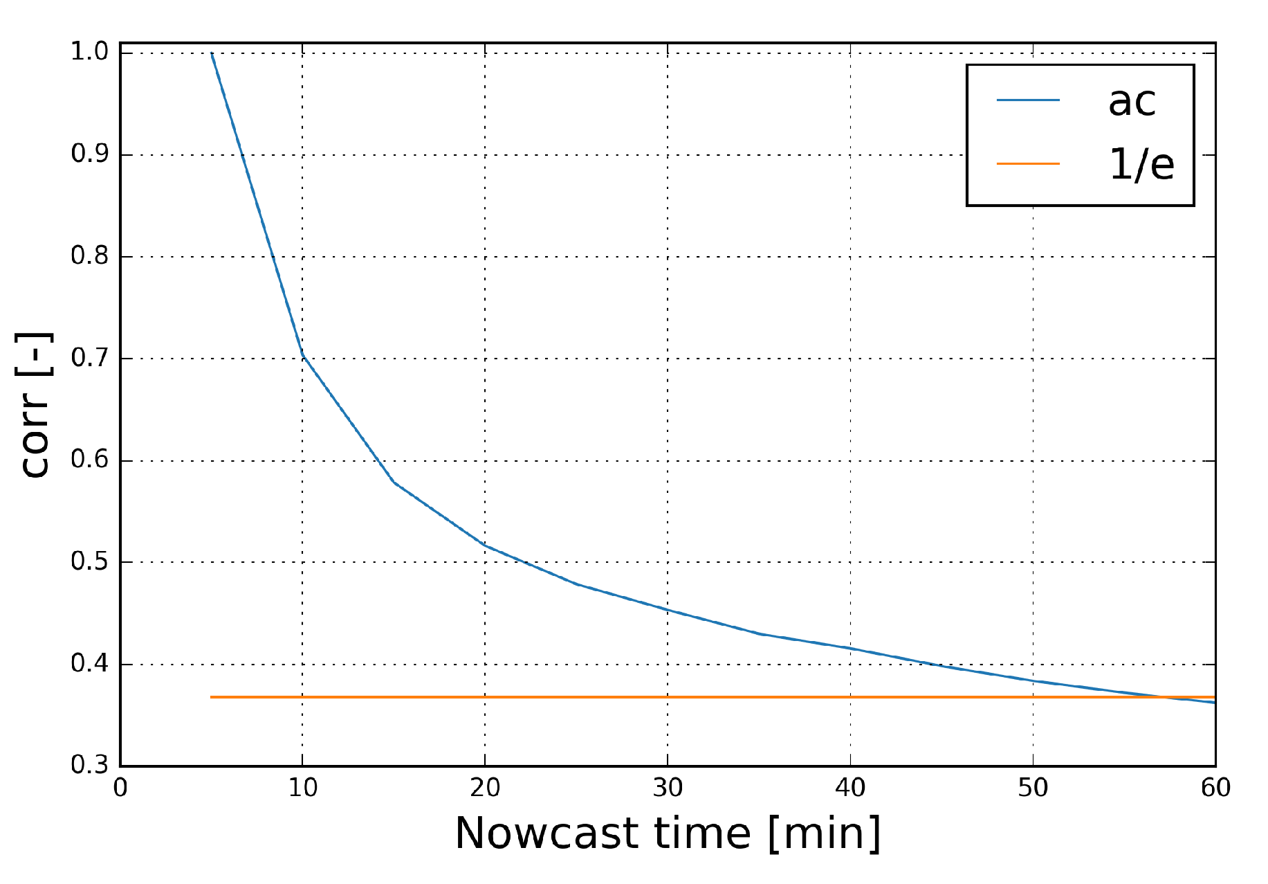
Before starting the discussion on the results, a preliminary consideration need to be made to understand both strenghts and limitations of nowcasts based on optical flow extrapolation techniques. All methods used (ST, SP, DR and LK) can fall into this category of course except the NN. Figure 4 shows the spatial autocorrelation of radar images as a function of the delay, in minutes, for 200 2017 “rainy” events, randomly chosen. As can be seen, the autocorrelation decays quickly but is appreciable (the orange line represents the inverse of the number of Nepero: ) up to a delay of about 60’. This can be taken as a limit of predictability for persistence, a particular case of optical flow with zero advection, and therefore it is expected the optical flow procedures to have non negligeable skills for up to one hour. For the same reason, 60’ is also the maximum delay that makes sense to use as input for any extrapolation procedure based on recent history. That is why both for the SP and NN procedure 12 images (at 5’ intervals) preceding the nowcast time were used as initial conditions.
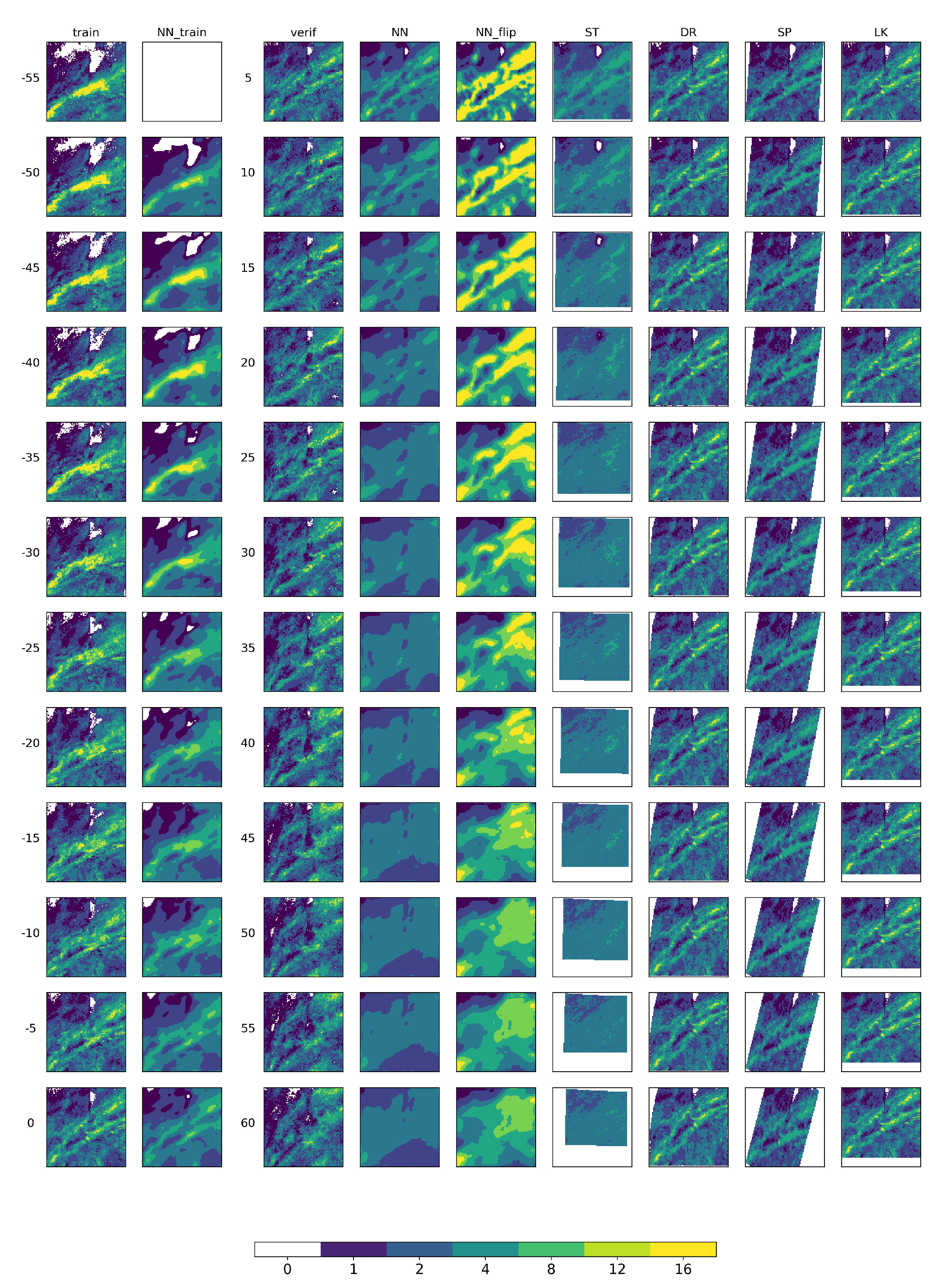
To clarify some aspects on which the discussion of the results will be based, in Figure 5 we show a sequence of images lasting one hour and related to the forecast of a precipitation event occurred on 8 January 2017. The first column shows the 12 frames that precede the forecast emission (train from minute −55 to 0), the second column (NN_train) shows the reconstruction of the precipitation field by the neural network. The network produces an estimate at each time step, starting from a zero field and gradually learning from the radar images provided. The third column (verif) shows instead the 12 images recorded by the radar and to be compared to in the following hour of forecast (minutes from 5 to 60). The following columns show, except the fourth (NN_flip) which we will discuss later, the nowcast for the procedures NN, ST, DR, SP and LK.
The domain of existence of the nowcast depends on the procedure used. The NN technique, being based on a neural network of generative type, returns a prediction for the whole domain while the SP and DR methods after the advective and extrapolative part try to “fill” the domain through interpolation, although generally this is never complete. Vice versa the ST and LK techniques, based only on the advection, have a field of existence just limited to the areas where the initial field has been “moved” while is undefined in the complementary areas. Note, in particular, in Figure 5 the frames for the forecast from 30’ onwards in which the area covered by the forecast is progressively reduced for all the forecasts except for NN. When comparing the performance of the different methods this fact is taken into account by evaluating the errors in the Domain of existence of each Single forecast (DS hereafter) and in the Domain resulting from their Intersection (DI henceforth). This problem is also highlighted by the extension of the domain covered by the radar data that is limited with respect to the typical advection speed of that climate zone and confirmed by the depicted event. This inconvenience could be avoided, or at least mitigated, considering a domain large enough to cover the central zone of greatest interest. To simplify the analysis of the results the discussion that follows is organized in subsections.
5.1. RMSE
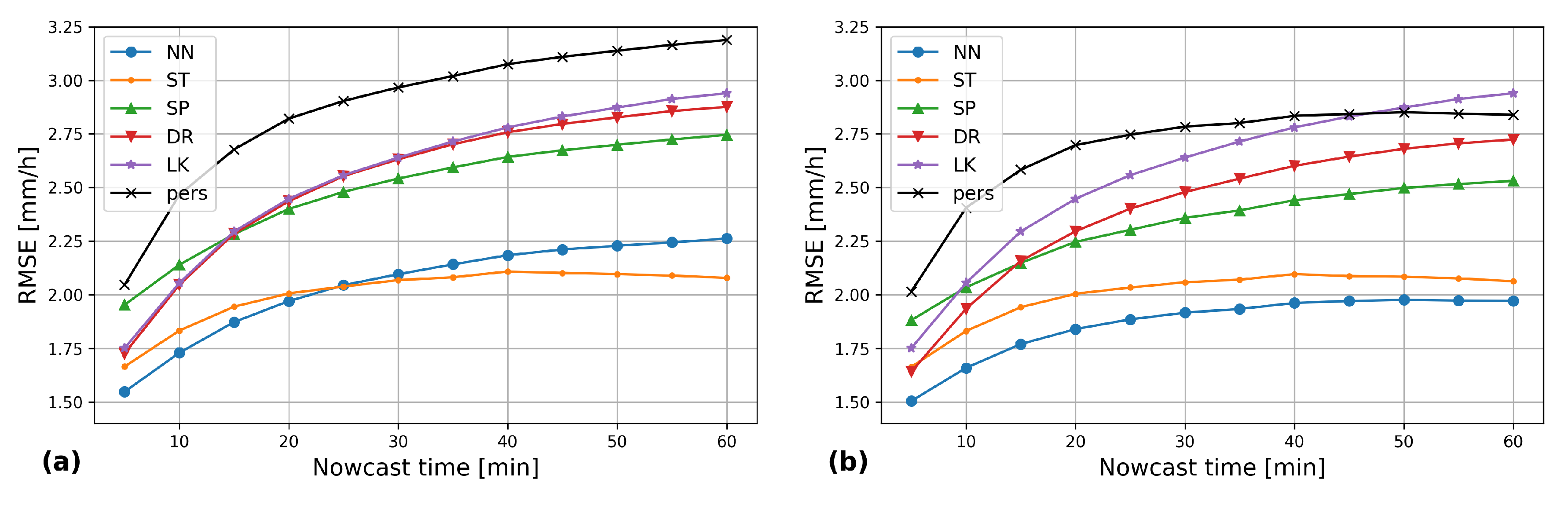
The use of RMSE metrics is not completely appropriate, for a field as discontinuous as precipitation. Nonetheless it provides an interesting “bulk” measure to compare the performance of the various methods. The box (a) of Figure 6 shows the RMSE of the averaged forecast for the whole year 2017, depending on the forecast time from 1’ to 60’, for the procedures NN, ST, SP, DR and persistence, evaluated on the DS domains. It is clear that for all techniques there is an added value compared to persistence that lasts for the entire duration of the forecast. NN and ST have an RMSE significantly lower than all the other techniques and in particular ST prevails over NN only in the second half hour. However, since the mean RMSE has been evaluated and then averaged again over different domains for each technique, a direct comparison is not possible. For this reason, in Figure 6, on box (b), is always shown the average RMSE evaluated only on the domain DI. In this case the trend is confirmed but NN prevails over the other techniques for all the 60’ of duration of the forecast. The slight prevalence of ST over NN in the second half hour forecast can be related to ST’s ability to incorporate the average effects of stochastic noise, whose influence increases with the forecasting time. On the other hand, NN has the clear advantage of providing a prediction for the entire domain covered by the radar. In addition this ST prevalence, as be shortly shown, disappears when the performance is evaluated using scores more suitable to assess the quality of the precipitation forecast, such as the MAE, r and, especially, the ETS.
5.2. MAE and Pearson Correlation Coefficient r
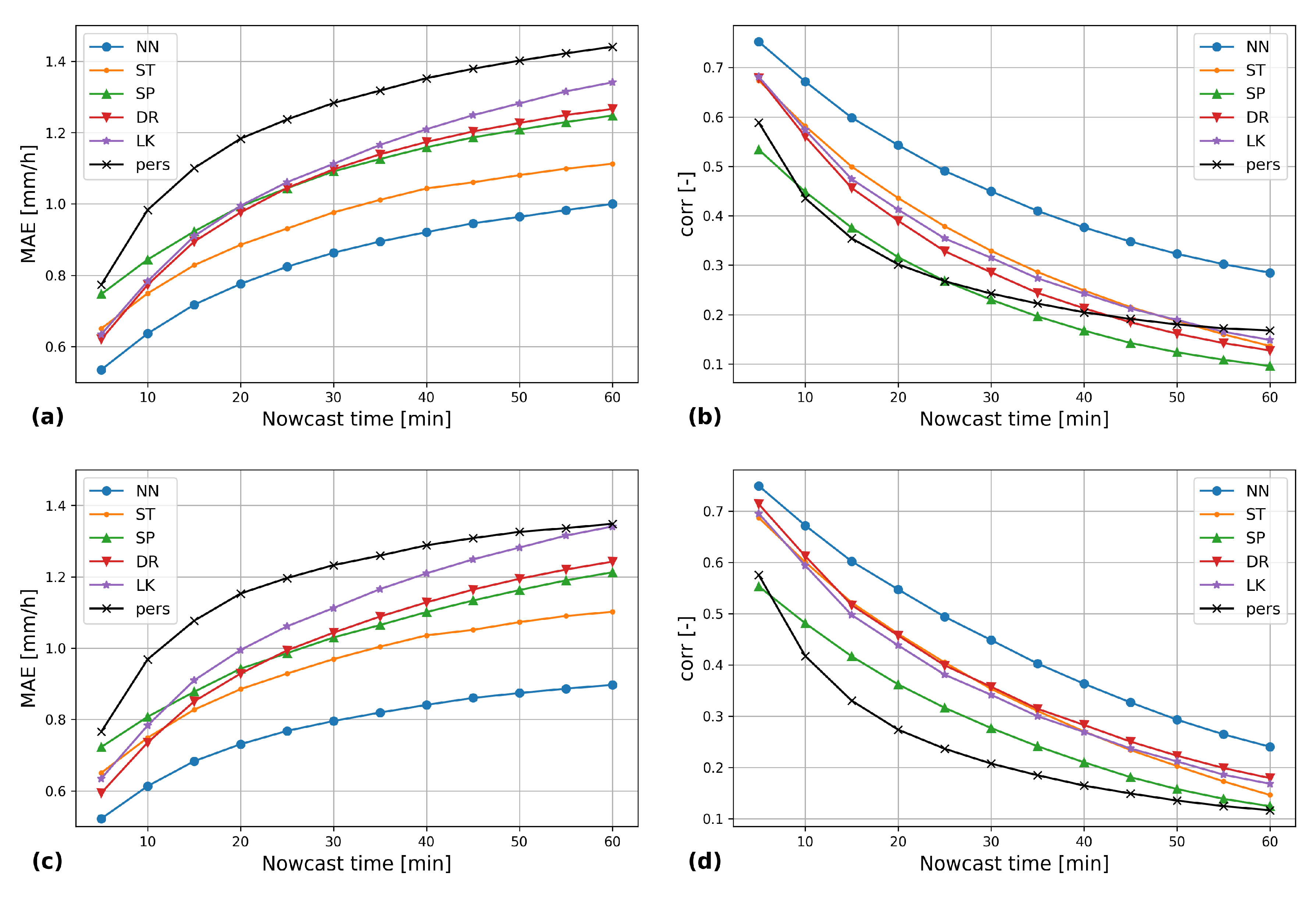
Figure 7 shows the values of the MAE and of the Pearson’s correlation coefficient r as a function of the forecast time, from 1’ to 60’, for the nowcast of the 5 procedures and for persistence, for 2017. The superiority of NN over all other procedures is clear, both in terms of MAE and of r, even when these were calculated over the DS domain (boxes (a) and (b)). To verify the robustness of the results obtained, we repeated the calculation of the MAE and r, limiting the analysis to the DI domain. The results are shown in boxes (c) and (d) of Figure 5. In this case too the performance of the NN method proved to be better than those of each of the others.
5.3. ETS
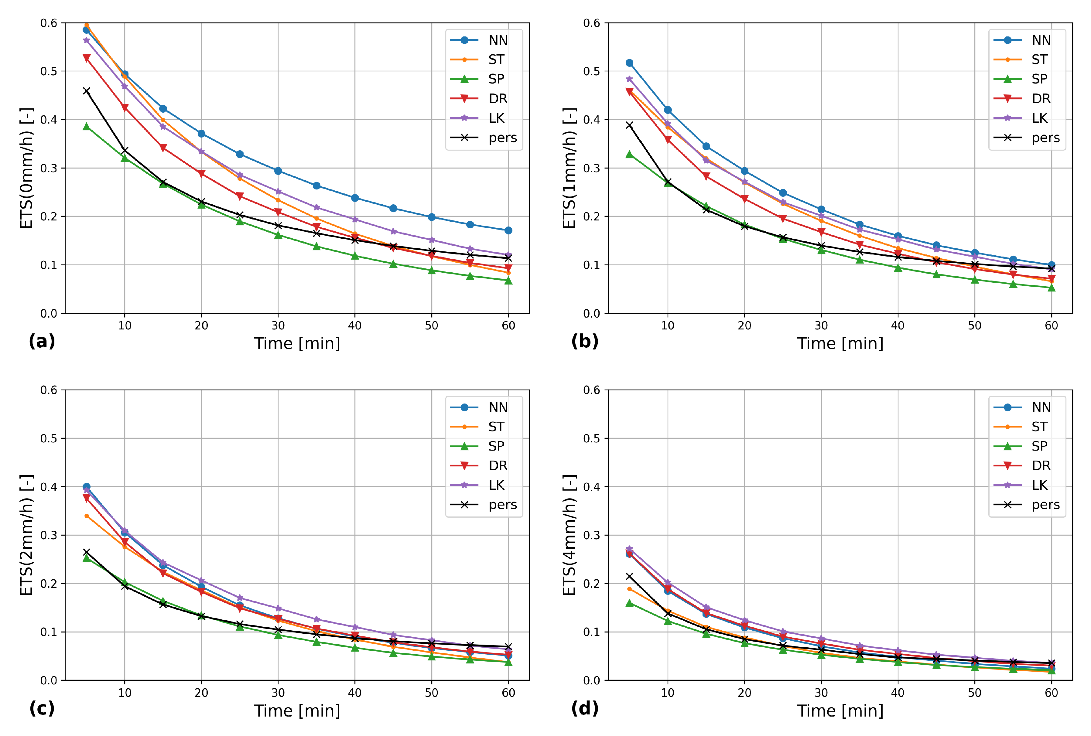
Figure 8 shows in boxes (a), (b), (c), (d) the ETS for the 0, 1, 2, 4 mm/h thresholds exceedance. While it is clear the advantage of the tested procedures with respect to persistence, the NN procedure stands out for the case of 0 mm/h (rain/no-rain) and 1 mm/h thresholds. For higher thresholds there is a slight prevalence of the LK method over all other procedures. However, the maximum values of ETS are significantly lower, as are the differences between the LK, NN and DR methods, which makes this lead not significant. The results reported in Figure 8 are obtained calculating the ETS in the DS domain (therefore different for each one), but the results obtained limiting the calculation to the common DI domain are basically identical and therefore not shown for brevity.
5.4. Skill Score
To have a measure of the accuracy of the nowcasting methods, for the entire duration of the forecast, we used two skill scores (SS) based on RMSE and MAE.
The accuracy is evaluated relatively to the persistence using the following espression:
where is the method for which the skill score is calculated. Similar formulas was used to calculate the SS(MAE). The values of the two SS obtained are summarized in Table 4. Looking at table, the plots and the discussion of the previous paragraph a clear superiority of the NN method is evident, despite the fact that both the RMSE and the MAE have been evaluated in the DS domain of each of the used methods. Once more, it is also worth to note that the only method able to produce a prediction on the entire radar domain is NN, while all others are limited to a portion of it, depending from the advection speed of the event and the forecast time. This is also the reason the SS(RMSE) for ST is slightly better than the one for NN (see discussion of Figure 6).
5.5. NN vs. ST
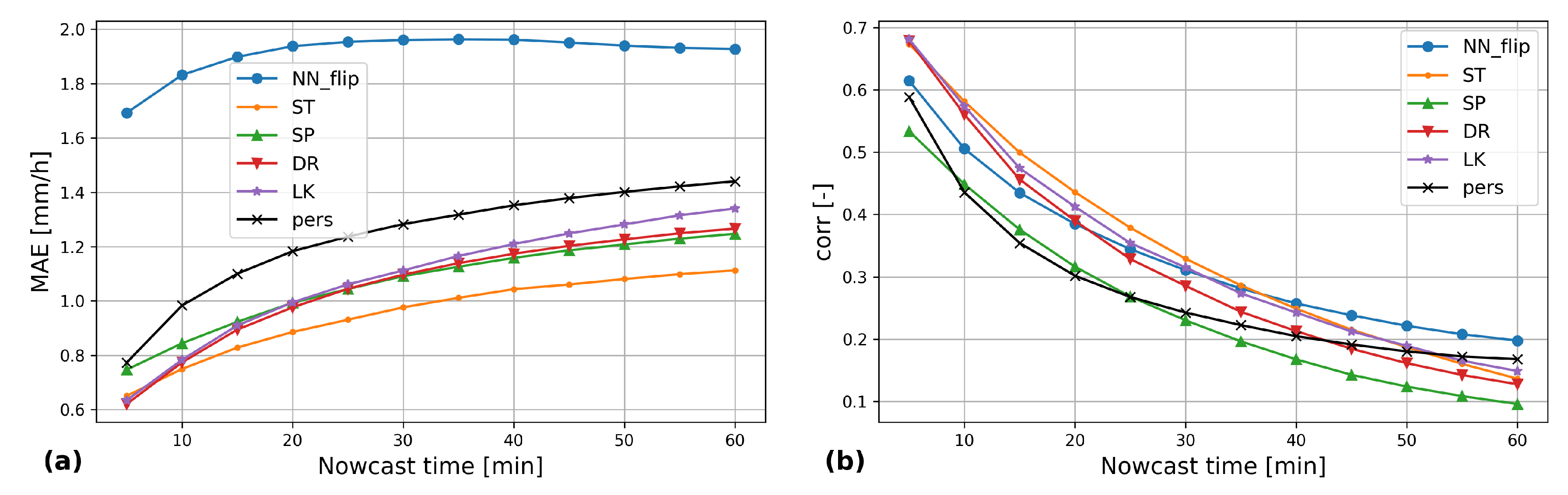
The results clearly show that the NN nowcast procedure, based on generative neural network, has a significantly better performance than all the algorithm that, to the best of our knowledge, represent the current state of the art. At least in the chosen configuration: a domain of relatively small size, compared to the typical advection speed of the climate zone where the radar used operates. To investigate the origin of this performance difference, the input data for the nowcast were flipped with respect to the increasing direction of latitude and longitude and the nowcast repeated throughout the year 2017. All methods based on optical flow are invariant with respect to this transformation.
Not so for NN, as demonstrated by the MAE and r shown in Figure 9. In particular from a quantitative point of view, it is clear that the nowcast for the data flipped in latitude and longitude are completely wrong (see MAE for NN_flip on box (a)) while those for the correlation coefficient worsen considerably but remain in line with those of the other methods, in particular for forecast times over 30’ (see box (b)). Most likely this result is an indication of the neural network “learning” correctly, from the three years of training data, the climatic characteristics of the phenomena related to the particular domain. The behavior of NN applied to the flipped data, with respect to those on the natural domain, can be verified by the analysis of the test case shown in Figure 5. Comparing the NN frames with the corresponding NN_flip (see the fifth column of images), the similarity of the two predicted patterns is clear and might be related to the NN advective component. Regarding the amount of rain, NN_flip provides much more intense precipitation, and this can be related to the generative component of the network. This is consistent with the considerably higher values of MAE and, at the same time, with the r values similar to the other procedures.
5.6. Space-Time Behavior of the Nowcast
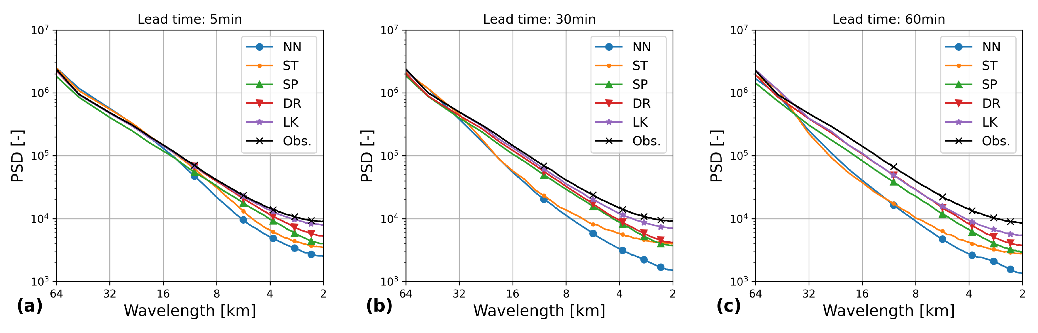
The improvement in performance achieved with NN brings in a reduction in the spatial detail of the forecast. This can be seen, from a qualitative standpoint, for the case shown in Figure 5, observing how the smoothing level of the solution NN increases with the lead time, more than for the other methods. Addressing the quantitative aspect, we calculated the spectral power density of the logarithmic transformation both for the measured and predicted fields In Figure 10 the results obtained by averaging the PSD on all the “rainy” events of 2017 for 5’, 30’ and 60’ lead times are shown on boxes (a), (b) and (c) respectively. NN starts to lose power already at a scale of about 16 km for the 5’ forecast. This loss of detail moves up to 32 km at 30’ lead time, and 48 km at 60’ lead time, in line with the results shown in [34] for the RainNet method.
This unintended feature of the NN forecast derives from the network optimization procedure which, while minimizing the loss function, devises "effective" smoothing the solution. The behavior, implicit at each 5’ forecast, is amplified by numerical diffusion as the forecast time progresses, because of the iterative nature of NN.
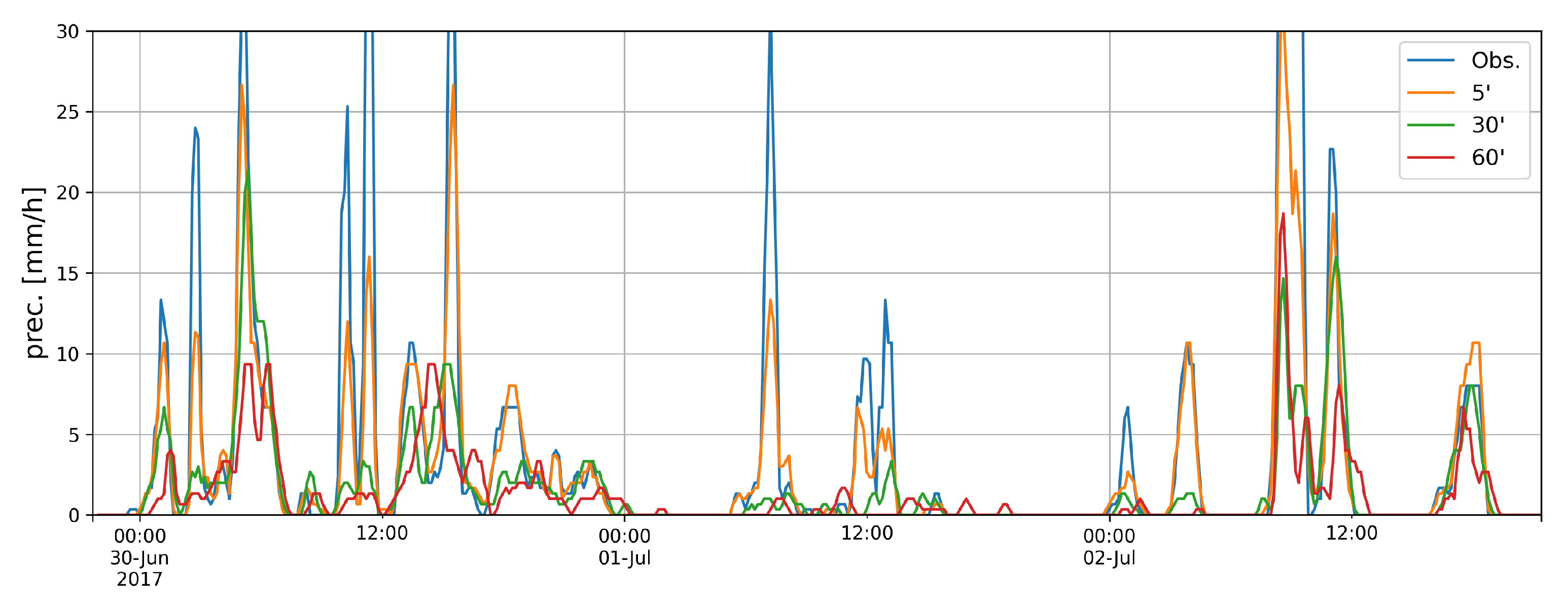
This is also reflected in NN’s reduced ability to predict extreme values. As an example, in Figure 11, a time series of precipitation data, for a severe event (29 June to 2 July 2017), is shown for the point of the radar nearest to Kyoto. The radar data estimation of precipitation in mm/h are shown along with the corresponding NN prediction, at lead times of 5’, 30’, and 60’. The smoothing effect of the forecast could be seen also here, but now over time. For events longer than an hour, in this case the first and third day of the event, the procedure is able to reproduce the evolution of the precipitation field even at lead times of 60’. The central part, instead, is poorly predicted as it lasts less then the minimum needed learning time. The power spectra tells us that this is caused by the pixel scale not being resolved. However, for hydrological applications, if the basin has a surface as large as the scales resolved by the nowcast, this effect is minimized since all points within the basin contribute to the runoff.
The increasing space-time “smoothness” of the NN forecast with lead times, is related to the increasing uncertainty of the forecast, an aspect which is out of the scope of the present paper, and on which we are currently working on as an extension of the present research.
6. Conclusions
In this work, a comparison of state-of-the-art methods for the nowcast of precipitation intensity derived from weather radar images and based on optical flow, with a deep learning methodology based on PredNet architecture, trained with a specific loss function, is presented.
The detailed analysis of this extensive test case proves that the proposed algorithm, based on a generative neural network architecture, is far superior to any other method representing, to the best of our knowledge, the state of the art for this subject. It must be said, according to a precautionary principle, that these conclusions cannot be generalized, a priori, to the nowcast of the images of another type of radar or a similar one positioned in a different geographical region. This limit originates from the small size of the domain covered by the radar, compared to the typical advection velocity obtained through the application of OF techniques.On the other hand, there is no valid reason the procedure used here could not be used in other domains and/or other radar types, after an appropriate learning phase, to produce similar encouraging results.
It would be certainly interesting to further develop the proposed concepts and methodologies. In that respect a modification of the architecture in order to formally separate the advective component from the source/sink in the generative branch of the network will be applied in an upcoming work. This should facilitate a transfer learning process and build a general model, able to interpret and predict radar measures, that can then be specialized onto specific instruments and/or different meteo/climatic regions. We also intend to study the potential for a probabilistic nowcast, estimating the spatial and temporal uncertainty that can be obtained from neural network model, for instance through a quantile regression and the use of a pinball loss function [35].
Author Contributions
M.M. and L.M. jointly conceived and designed the methodologies, performed the analysis and wrote the paper. All authors have read and agreed to the published version of the manuscript.
Funding
This work was financed by the project “Tessuto Digitale Metropolitano” funded by the regional agency Sardegna Ricerche (POR FESR 2014-2020, Azione 1.2.2) and by Sardinian Regional Authorities.
Acknowledgments
The authors would like to thank Ryoma Sato of Kyoto University for sharing his scripts, necessary to download the dataset.
Conflicts of Interest
The authors declare no conflict of interest.
References
- Bartholmes, J.; Todini, E. Coupling meteorological and hydrological models for flood forecasting. Hydrol. Earth Syst. Sci. Discuss. 2005, 9, 333–346. [Google Scholar] [CrossRef] [Green Version]
- Tran, Q.K.; Song, S.K. Computer Vision in Precipitation Nowcasting: Applying Image Quality Assessment Metrics for Training Deep Neural Networks. Atmosphere 2019, 10, 244. [Google Scholar] [CrossRef] [Green Version]
- Heye, A.; Venkatesan, K.; Cain, J. Precipitation nowcasting: Leveraging deep recurrent convolutional neural networks. Proc. Cray User Group (CUG) 2017, 2017, 1–8. [Google Scholar]
- Yu, W.; Nakakita, E.; Kim, S.; Yamaguchi, K. Improvement of rainfall and flood forecasts by blending ensemble NWP rainfall with radar prediction considering orographic rainfall. J. Hydrol. 2015, 531, 494–507. [Google Scholar] [CrossRef]
- Verbunt, M.; Walser, A.; Gurtz, J.; Montani, A.; Schär, C. Probabilistic Flood Forecasting with a Limited-Area Ensemble Prediction System: Selected Case Studies. J. Hydrometeorol. 2007, 8, 897–909. [Google Scholar] [CrossRef]
- Corral, C.; Sempere-Torres, D.; Revilla, M.; Berenguer, M. A semi-distributed hydrological model using rainfall estimated by radar; application to Mediterranean basins. Phys. Chem. Earth B 2000, 25, 1133–1136. [Google Scholar] [CrossRef]
- Knöll, P.; Zirlewagen, J.; Scheytt, T. Using radar-based quantitative precipitation data with coupled soil- and groundwater balance models for stream flow simulation in a karst area. J. Hydrol. 2020, 586, 24884. [Google Scholar] [CrossRef]
- Collier, C.G. On the propagation of uncertainty in weather radar estimates of rainfall through hydrological models. Meteorol. Appl. 2009, 16, 35–40. [Google Scholar] [CrossRef]
- Nguyen, D.H.; Bae, D.H. Correcting mean areal precipitation forecasts to improve urban flooding predictions by using long short-term memory network. J. Hydrol. 2020, 584, 124710. [Google Scholar] [CrossRef]
- Ayzel, G.; Heistermann, M.; Winterrath, T. Optical flow models as an open benchmark for radar-based precipitation nowcasting (rainymotion v0. 1). Geosci. Model Dev. 2019, 12, 1387–1402. [Google Scholar] [CrossRef] [Green Version]
- Reyniers, M. Quantitative Precipitation Forecasts Based on Radar Observations: Principles, Algorithms and Operational Systems; Institut Royal Météorologique de Belgique: Brussel, Belgium, 2008. [Google Scholar]
- Woo, W.C.; Wong, W.K. Operational application of optical flow techniques to radar-based rainfall nowcasting. Atmosphere 2017, 8, 48. [Google Scholar] [CrossRef] [Green Version]
- Bechini, R.; Chandrasekar, V. An enhanced optical flow technique for radar nowcasting of precipitation and winds. J. Atmos. Ocean. Technol. 2017, 34, 2637–2658. [Google Scholar] [CrossRef]
- Lucas, B.D.; Kanade, T. An iterative image registration technique with an application to stereo vision. In Proceedings of the Seventh International Joint Conference on Artificial Intelligence (IJCAI ’81), Vancouver, BC, Canada, 24–28 August 1981; pp. 674–679. [Google Scholar]
- Wong, M.; Wong, W.; Lai, E.S. From SWIRLS to RAPIDS: Nowcast applications development in Hong Kong. In Proceedings of the PWS Workshop on Warnings of Real-Time Hazards by Using Nowcasting Technology, Sydney, Australia, 9–13 October 2006. [Google Scholar]
- Shi, J. Good features to track. In Proceedings of the IEEE Conference on Computer Vision and Pattern Recognition, Seattle, WA, USA, 21–23 June 1994; pp. 593–600. [Google Scholar]
- Schneider, P.; Eberly, D.H. Geometric Tools for Computer Graphics; Elsevier Science: Cambridge, MA, USA, 2003. [Google Scholar]
- Seed, A. A dynamic and spatial scaling approach to advection forecasting. J. Appl. Meteorol. 2003, 42, 381–388. [Google Scholar] [CrossRef]
- Shi, X.; Chen, Z.; Wang, H.; Yeung, D.Y.; Wong, W.K.; Woo, W.C. Convolutional LSTM network: A machine learning approach for precipitation nowcasting. In Advances in Neural Information Processing Systems; Curran Associates, Inc.: Red Hook, NY, USA, 2015; pp. 802–810. [Google Scholar]
- Shi, X.; Gao, Z.; Lausen, L.; Wang, H.; Yeung, D.Y.; Wong, W.K.; Woo, W.C. Deep learning for precipitation nowcasting: A benchmark and a new model. In Advances in Neural Information Processing Systems; Curran Associates, Inc.: Red Hook, NY, USA, 2017; pp. 5617–5627. [Google Scholar]
- Sato, R.; Kashima, H.; Yamamoto, T. Short-Term Precipitation Prediction with Skip-Connected PredNet. In Proceedings of the 27th International Conference on Artificial Neural Networks (ICANN 2018), Rhodes, Greece, 4–7 October 2018; Springer: Cham, Switzerland, 2018; pp. 373–382. [Google Scholar]
- Ayzel, G.; Heistermann, M.; Sorokin, A.; Nikitin, O.; Lukyanova, O. All convolutional neural networks for radar-based precipitation nowcasting. Procedia Comput. Sci. 2019, 150, 186–192. [Google Scholar] [CrossRef]
- Lotter, W.; Kreiman, G.; Cox, D. Deep predictive coding networks for video prediction and unsupervised learning. arXiv 2016, arXiv:1605.08104. [Google Scholar]
- Pulkkinen, S.; Nerini, D.; Pérez Hortal, A.A.; Velasco-Forero, C.; Seed, A.; Germann, U.; Foresti, L. Pysteps: An open-source Python library for probabilistic precipitation nowcasting (v1. 0). Geosci. Model Dev. 2019, 12, 4185–4219. [Google Scholar] [CrossRef] [Green Version]
- Bradski, G.; Kaehler, A. Learning OpenCV: Computer vision with the OpenCV library; O’Reilly Media, Inc.: Sebastopol, CA, USA, 2008. [Google Scholar]
- Wolberg, G. Digital Image Warping; IEEE Computer Society Press: Los Alamitos, CA, USA, 1990; Volume 10662. [Google Scholar]
- Bouguet, J.Y. Pyramidal implementation of the affine lucas kanade feature tracker description of the algorithm. Intel Corp. 2001, 5, 4. [Google Scholar]
- Laroche, S.; Zawadzki, I. Retrievals of horizontal winds from single-Doppler clear-air data by methods of cross correlation and variational analysis. J. Atmos. Ocean. Technol. 1995, 12, 721–738. [Google Scholar] [CrossRef] [Green Version]
- Germann, U.; Zawadzki, I. Scale-dependence of the predictability of precipitation from continental radar images. Part I: Description of the methodology. Mon. Weather Rev. 2002, 130, 2859–2873. [Google Scholar] [CrossRef]
- Ruzanski, E.; Chandrasekar, V.; Wang, Y. The CASA nowcasting system. J. Atmos. Ocean. Technol. 2011, 28, 640–655. [Google Scholar] [CrossRef]
- Pulkkinen, S.; Chandrasekar, V.; Harri, A.M. Fully spectral method for radar-based precipitation nowcasting. IEEE J. Sel. Top. Appl. Earth Obs. Remote Sens. 2019, 12, 1369–1382. [Google Scholar] [CrossRef]
- Van Rossum, G.; Drake, F.L. Python 3 Reference Manual; CreateSpace: Scotts Valley, CA, USA, 2009. [Google Scholar]
- Paszke, A.; Gross, S.; Massa, F.; Lerer, A.; Bradbury, J.; Chanan, G.; Killeen, T.; Lin, Z.; Gimelshein, N.; Antiga, L.; et al. PyTorch: An Imperative Style, High-Performance Deep Learning Library. In Advances in Neural Information Processing Systems 32; Wallach, H., Larochelle, H., Beygelzimer, A., D’Alché-Buc, F., Fox, E., Garnett, R., Eds.; Curran Associates, Inc.: Red Hook, NY, USA, 2019; pp. 8024–8035. [Google Scholar]
- Ayzel, G.; Tobias, S.; Maik, H. RainNet v1.0: A convolutional neural network for radar-based precipitation nowcasting. Geosci. Model Dev. 2020. in review. [Google Scholar] [CrossRef]
- Petersik, P.J.; Dijkstra, H.A. Probabilistic Forecasting of El Niño Using Neural Network Models. Geophys. Res. Lett. 2020, 47. [Google Scholar] [CrossRef]
Figure 1.
PredNet architecture: in the left the general architecture with the Discriminator blocks and the Generator blocks, in the right details of blocks.
Figure 1.
PredNet architecture: in the left the general architecture with the Discriminator blocks and the Generator blocks, in the right details of blocks.

Figure 2.
On the left the map of Japan in which is highlighted the area shown in detail on the right that represents the domain covered by the Japanese meteorological radar whose data is used in this work.
Figure 2.
On the left the map of Japan in which is highlighted the area shown in detail on the right that represents the domain covered by the Japanese meteorological radar whose data is used in this work.

Figure 3.
Climate data of monthly average temperature (a) and precipitation (b) for three meteorological stations in the domain.
Figure 3.
Climate data of monthly average temperature (a) and precipitation (b) for three meteorological stations in the domain.

Figure 4.
Autocorrelation of precipitation field as function of the delay expressed in minutes for a sample of 200 “rainy” events.
Figure 4.
Autocorrelation of precipitation field as function of the delay expressed in minutes for a sample of 200 “rainy” events.

Figure 5.
Frame sequence illustrating the mode of operation of the different nowcast techniques calculated for the one-hour forecast starting on January 8 at 16:25 UTM. See the text for a detailed description of the figure.
Figure 5.
Frame sequence illustrating the mode of operation of the different nowcast techniques calculated for the one-hour forecast starting on January 8 at 16:25 UTM. See the text for a detailed description of the figure.

Figure 6.
Average RMSE as function of the forecast time from 1’ to 60’, for all nowcast methods and persistence (2017). In box (a) the indicators are evaluated in the DS domain, in (b) the same indicators are calculated in DI.
Figure 6.
Average RMSE as function of the forecast time from 1’ to 60’, for all nowcast methods and persistence (2017). In box (a) the indicators are evaluated in the DS domain, in (b) the same indicators are calculated in DI.

Figure 7.
As in the previous figure for MAE and Pearson’s correlation coefficient. First row of plots (boxes (a) and (b)) shows results evaluated in the domain DS, second row (boxes (c) and (d)) those in DI.
Figure 7.
As in the previous figure for MAE and Pearson’s correlation coefficient. First row of plots (boxes (a) and (b)) shows results evaluated in the domain DS, second row (boxes (c) and (d)) those in DI.

Figure 8.
ETS, for 0, 1, 2, 4 mm/h thresholds shown on boxes (a), (b), (c), (d) respectively, as function of the forecast time from 1’ to 60’, for all nowcast methods and persistence, for 2017.
Figure 8.
ETS, for 0, 1, 2, 4 mm/h thresholds shown on boxes (a), (b), (c), (d) respectively, as function of the forecast time from 1’ to 60’, for all nowcast methods and persistence, for 2017.

Figure 9.
As in Figure 7. On box (a) the MAE and on box (b) the correlation coefficient of Pearson r as a function of the forecast time from 1 to 60 min, this time for the nowcast obtained by inverting the axes of longitude and latitude of the domain. The results for NN, the only ones that differ from those shown in Figure 7, are indicated with NN_flip.

Figure 10.
Power spectral density averaged over all the precipitation events of 2017, for times of forecast of 5’, 30’ and 60’ on boxes (a), (b) and (c) respectively.
Figure 10.
Power spectral density averaged over all the precipitation events of 2017, for times of forecast of 5’, 30’ and 60’ on boxes (a), (b) and (c) respectively.

Figure 11.
Time series of an event of intense precipitation occurred above Kyoto in the period from the 29 of June to the 2 of July 2017. Radar observations and corresponding NN forecasts at lead times of 5’, 30’ and 60’ are shown.
Figure 11.
Time series of an event of intense precipitation occurred above Kyoto in the period from the 29 of June to the 2 of July 2017. Radar observations and corresponding NN forecasts at lead times of 5’, 30’ and 60’ are shown.


Table 1.
PredNet tensors: size of the tensors for the different levels of the PredNet architecture expressed as (channels, width, height).
Table 1.
PredNet tensors: size of the tensors for the different levels of the PredNet architecture expressed as (channels, width, height).
| Level l | ||||
|---|---|---|---|---|
| 0 | (1, 96, 96) | (1, 96, 96) | (2, 96, 96) | (1, 96, 96) |
| 1 | (16, 48, 48) | (16, 48, 48) | (32, 48, 48) | (16, 48, 48) |
| 2 | (32, 24, 24) | (32, 24, 24) | (64, 24, 24) | (32, 24, 24) |
| 3 | (64, 12, 12) | (64, 12, 12) | (128, 12, 12) | (64, 12, 12) |
Table 2.
Table of correspondence between the colors of the radar image representation and the precipitation intensity.
Table 2.
Table of correspondence between the colors of the radar image representation and the precipitation intensity.
| Index | Color (RGB) | Rain (mm/h) |
|---|---|---|
| 0 | (255, 255, 255) | 0 |
| 1 | (236, 254, 252) | 1 |
| 2 | (196, 254, 252) | 2 |
| 3 | (156, 234, 252) | 4 |
| 4 | (156, 218, 252) | 8 |
| 5 | (180, 198, 252) | 12 |
| 6 | (180, 254, 156) | 16 |
| 7 | (180, 234, 156) | 24 |
| 8 | (164, 218, 156) | 32 |
| 9 | (252, 254, 156) | 40 |
| 10 | (252, 234, 156) | 48 |
| 11 | (252, 218, 156) | 56 |
| 12 | (252, 190, 196) | 64 |
| 13 | (252, 158, 156) | 80 |
| 14 | (228, 158, 164) | 100 |
Table 3.
Comparison of the number of images processed by the different methodologies to obtain a forecast of 12 steps, equivalent to 1 h.
Table 3.
Comparison of the number of images processed by the different methodologies to obtain a forecast of 12 steps, equivalent to 1 h.
| Method | Past Steps | Forecast Steps |
|---|---|---|
| NN | 12 | 12 |
| ST | 3 | 12 |
| SP | 12 | 12 |
| DR | 2 | 12 |
| LK | 2 | 12 |
Table 4.
RMSE- and MAE-based skill scores relative to the persistence for all nowcasting method used. Both RMSE and MAE are calculated within the domain DS of existence of each nowcast.
Table 4.
RMSE- and MAE-based skill scores relative to the persistence for all nowcasting method used. Both RMSE and MAE are calculated within the domain DS of existence of each nowcast.
| Method | SS (RMSE) | SS (MAE) |
|---|---|---|
| NN | 0.29 | 0.32 |
| ST | 0.30 | 0.23 |
| SP | 0.13 | 0.14 |
| DR | 0.12 | 0.15 |
| LK | 0.11 | 0.14 |
© 2020 by the authors. Licensee MDPI, Basel, Switzerland. This article is an open access article distributed under the terms and conditions of the Creative Commons Attribution (CC BY) license (http://creativecommons.org/licenses/by/4.0/).
Share and Cite
MDPI and ACS Style
Marrocu, M.; Massidda, L. Performance Comparison between Deep Learning and Optical Flow-Based Techniques for Nowcast Precipitation from Radar Images. Forecasting 2020, 2, 194-210. https://0-doi-org.brum.beds.ac.uk/10.3390/forecast2020011
AMA Style
Marrocu M, Massidda L. Performance Comparison between Deep Learning and Optical Flow-Based Techniques for Nowcast Precipitation from Radar Images. Forecasting. 2020; 2(2):194-210. https://0-doi-org.brum.beds.ac.uk/10.3390/forecast2020011
Chicago/Turabian StyleMarrocu, Marino, and Luca Massidda. 2020. "Performance Comparison between Deep Learning and Optical Flow-Based Techniques for Nowcast Precipitation from Radar Images" Forecasting 2, no. 2: 194-210. https://0-doi-org.brum.beds.ac.uk/10.3390/forecast2020011