Goes-13 IR Images for Rainfall Forecasting in Hurricane Storms


1
Water Research Center, Centro de Investigaciones del Agua-Queretaro (CIAQ), Young Water Professionals, International Water Association-Mexico, Universidad Autonoma de Queretaro, Queretaro 76010, Mexico
2
Water Research Center, Centro de Investigaciones del Agua-Queretaro (CIAQ), International Flood Initiative, Latin-American and the Caribbean Region (IFI-LAC), Intergovernmental Hydrological Programme (IHP-UNESCO), Universidad Autonoma de Queretaro, Queretaro 76010, Mexico
*
Author to whom correspondence should be addressed.
Forecasting 2020, 2(2), 85-101; https://0-doi-org.brum.beds.ac.uk/10.3390/forecast2020005
Submission received: 16 September 2019
/
Revised: 4 April 2020
/
Accepted: 29 April 2020
/
Published: 30 April 2020
Abstract
:Currently, it is possible to access a large amount of satellite weather information from monitoring and forecasting severe storms. However, there are no methods of employing satellite images that can improve real-time early warning systems in different regions of Mexico. The auto-estimator is the most commonly used technique that was developed for specific locations in the United States of America (32–49° latitude) for the type of convective storms. However, the estimation of precipitation intensities for meteorological conditions in tropic latitudes, using the auto-estimator technique, needs to be re-adjusted and calibrated. It is necessary to improve this type of technique that allows decision-makers to have hydro-informatic tools capable of improving early warning systems in tropical regions (15–25° Mexican tropic latitude). The main objective of the work is to estimate rainfall from satellite imagery in the infrared (IR) spectrum from the Geostationary Operational Environmental Satellite (GOES), validating these estimates with a network of surface rain gauges. Using the GOES-13 IR images every 15 min and using the auto-estimator, a downscaling of six hurricanes was performed from which surface precipitation events were measured. The two main difficulties were to match the satellite images taken every 15 min with the surface data measured every 10 min and to develop a program in C+ that would allow the systematic analysis of the images. The results of this work allow us to get a new adjustment of coefficients in a new equation of the auto-estimator, valid for rain produced by hurricanes, something that has not been done until now. Although no universal relationship has been found for hurricane rainfall, it is evident that the original formula of the auto-estimator technique needs to be modified according to geographical latitude.
1. Introduction
The measurement of the space–time variability of rainfall is essential for the progress of hydrologic studies, such as the water balance in a watershed, or the execution of projects and actions related to urban development in the field of hydraulic networks [1,2]. There is an increasing demand to improve rainfall estimates from satellite systems on a different range of scales in time and space. Remote sensing of the earth and its atmosphere in the infrared spectrum has become a mainstay of environmental monitoring for weather and climate [3]. The trend towards increasingly new applications in the field of hydrometeorology requires precise estimates of rainfall for global or local coverage [4,5,6]. Also, the new meteorological radar systems with improved beam resolution have increased signal-noise sensitivity. In fact, one of the most important limits of hydrological prediction is due to the low resolution of the input of hydrological models. This input is given by the measurements of the rain-gauge, so a dense network rain-gauge would allow the progress in radar rainfall estimates [7]. In any case, it is of great importance to have the appropriate characteristics of the passive microwave radiometers and the computational capacity to analyze the information retrieved from precipitation events [8,9]. In the case of radars, the algorithms to know the rain-rate or the intensity of the rainfall (RR) must be calibrated for a specific geographical location. It is also very important to know the frequencies in which the algorithms derive RR. Usually, the advanced microwave sounding radiometers (AMSR) measure at 6.9, 7.3, and 10.65 GHz [10]. For tropical regions, it could be from 10 to 150 GHz [11]. Radar measurements are an excellent way to develop warning systems; however, not all the countries of Latin-American and the Caribbean (LAC) have access to radar data or automatic telemetric rain-gauges. In this region, hurricanes are undoubtedly the most extreme events to be studied. Significant progress has already been made in implementing the monitoring of monsoon and tropical cyclone rainfall. For example, in India, a new technique has been developed to estimate rainfall on a very fine scale (hourly rain rate), using the infrared (IR) and water vapor (WV 6.7 μm) channel from satellite images. However, eventually, these values need to be compared with values measured on a radar [12]. The useful images to report cloud coverage during the day are of 0.6–1.6 μm (visible), 3.9–7.3 μm (infra-red/water vapor), and 8.7–13.4 μm (thermal images). However, the access and use of satellite images are promising in America for the LAC region with the Geostationary Operational Environmental Satellite (GOES) and the Meteosat for Africa. Meteosat is a geostationary weather satellite launched by the European Space Agency (ESA). In Florida, USA, the stream-flow simulated by satellite rainfall data was slightly better than when driven by rain-gauge data and was similar to the case of using radar data, reflecting the potential applications of satellite rainfall in basin-scale hydrologic modeling [13]. These methodologies use the brightness temperature of satellite images and then transform that brightness temperature into cold cloud temperature. Finally, the brightness temperature is transformed into precipitation intensity [14,15]. Geostationary satellites are especially important for their unique ability to simultaneously observe the atmosphere and its cloud cover from the global scale down to the storm scale at high resolution in both time (every 15 min) and space (1–4 km) [16]. A feature of the geo-stationary satellite is that it measures the amount of energy emitted by the atmosphere. The infrared sensors recorded the thermal properties of the Earth’s soil and ocean surface [17]. The top of the cold clouds is the main focus of the IR sensors in order to get rainfall quantification. There are a lot of satellite images available for tracking and forecasting extreme storms. However, in Mexico, since there is no extensive radar coverage, it is necessary to use satellite images to forecast rainfall intensities during the trajectory of hurricanes. The GOES-13 orbits the Earth at an altitude of approximately of 35 thousand kilometers above the equator; at this altitude, the satellite speed is equal to the angular speed of the Earth. The satellite rotates 360° in 24 h, this characteristic allows us to have constant monitoring of the same area, and in this case, the whole Mexican territory is monitored all day long at a 15-min frequency. The temperature of the cloud top can be estimated by the brightness temperature value of the image from the satellite in the infrared (IR) channel. This is the satellite is used in Mexico to visualize convective storms and hurricanes. A total of five geostationary satellites provide operational imagery: these currently include the Meteosat Second Generation satellites (MSG) from the European Organization for the Exploitation of Meteorological Satellites (EUMETSAT), two Geostationary Operational Environmental Satellites (GOESs) and the Japanese Multifunctional Transport Satellite (MTSAT) series [18]. However, the National Weather Service (Servicio Meteorologico Nacional Mexico, SMN) and the Mexican Space Agency (AEM), through an agreement signed in 2016 with the National Weather Service, USA (NWS), have access to GOES images. This allows the use of images with all their characteristics and all their attributes.
The most recognized methodology to estimate rainfall intensity from IR images was developed by Vicente et al. [19]. This methodology was applied for deep convection storms in the plains of the United States of America (32–49° latitude). Those locations are significantly different in latitude, longitude, and topographic conditions from those located in the tropical areas (15–25° Mexican tropic latitude). In order to apply this method in the Mexican territory, an adjustment to the formula proposed by Vicente et al. [19] is required. It is also relevant to develop this type of regionalization especially for deep convection storms, “convective systems which produce the greatest rainfall intensity”; these storms occur when the environment, specifically a parcel of air mass above the ground and under the cloud top, begins to get colder and starts to expand [20]. Kalinga and Gan [13] introduced rain and no-rain discrimination in their study, improving the estimates from IR imagery; in this case, the value of the discrimination brightness temperature was 109. At this brightness temperature value, we can observe rainfall intensity measured by rain gauges. It is important to mention that, to date, the algorithm proposed by Vicente et al. [19] only applies to convective storms. The use of this equation should be reviewed if it is to be applied to hurricane storms. The aim of this work is based on the development of a new equation for each case study from IR satellite images. Using GOES 13 images and information from automatic rain-gauge stations (MGS). As already mentioned, the brightness temperature value of the image is converted to temperature and then to precipitation intensity.
This paper is organized according to the following lineaments. Section 2 presents the imagery processing based on the brightness temperature value from the geo-localization of the zone of study (in the IR channel) and to get the brightness temperature values from a convective storm, also to recollect rain gauge data (rainfall inferred from IR satellite data) and validate the estimations with gauges measurements (time-lapse desegregation of satellite series). Then, six case examples are briefly described in Section 3. The first one, Hurricane Dean, on 21 August 2007, and the second, Hurricane Ernesto, with satellite images from 9 August 2012. These hurricanes were selected because they were the most intense in recent years. These case studies allow us to prove the limitations of the auto-estimator technique, with respect to the limit of rainfall rate (RR) to be considered. Section 4 presents a spatial-temporal description of the hurricanes analyzed. Based on the results of estimating precipitation intensity during a hurricane, the validity of the formula proposed by Vicente et al. [19] is discussed. The last section summarizes the main results of the research.
2. Materials and Methods
2.1. The Auto-Estimator in Tropical Regions
The auto-estimator is the most commonly used technique in the forecasting of rainfall intensity estimation from satellite images. However, it was developed for specific locations at 32–49° latitude, and only for convective storms. Nevertheless, the estimation of rainfall intensities for meteorological conditions in tropic latitudes, using the auto-estimator technique, needs to be re-adjusted and calibrated. First, hurricane events are selected with information available from GOES images and MGS surface data. Then, the satellite images are processed to get the brightness temperature values of each pixel. Then, using the original auto-estimator equation and coefficients, the brightness temperature is transformed into cloud top temperature, and the RR–satellite image is calculated. The next step is to match these obtained values with the surface data from RR–MGS. To carry out this comparison, it is necessary to disaggregate the rainfall data at the same time intervals. The comparative of the RR values allows us to know if the original formulation of the auto-estimator can properly forecast the RR. By applying the logarithmic conversion, it is possible to convert the auto-estimator equation into a linear expression, and thus to calculate the two coefficient (parameters) by multiple regression. In this way, two new parameters of the auto-estimator equation are calculated from the hurricanes analyzed. It can also be solved through B-spline estimation or least squares [21] getting the same set of results. Next, a regionalization of all the parameters that are obtained in this way is carried out and these are plotted in a Mexico map. Finally, a validation of the new auto-estimator coefficients is carried out with data from other hurricanes.
2.2. Imagery Treatment Processing
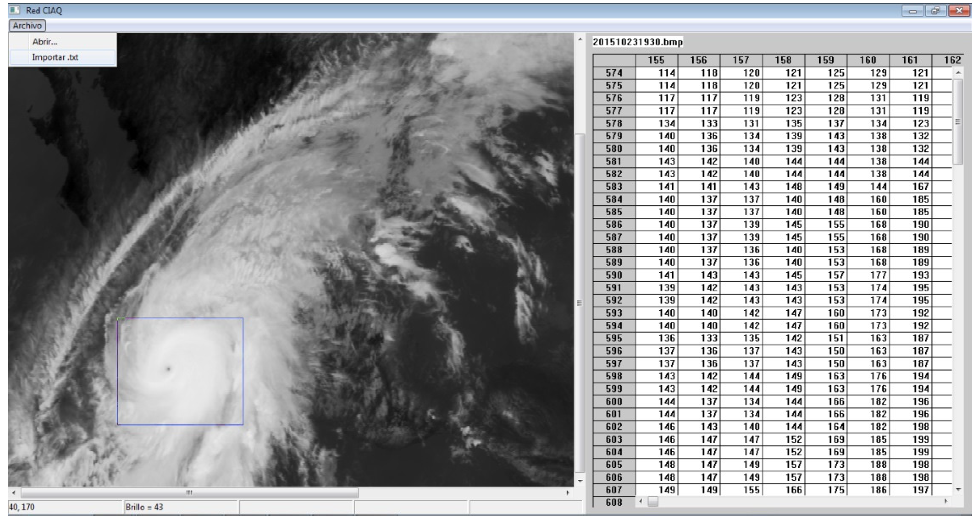
In Mexico, the SMN has records of MGS rain-gauges and has a receiving station of the IR images from GOES-13 with a frequency of approximately 15 min. All this data, MGS and image records include a period of 13 years. In order to assign each pixel, its digital level value between 0 and 255, according to its resolution of 8 bits. The first step is to obtain the brightness temperature value from a convective storm (in the IR channel), geo-localize the zone of study, as well as to recollect rain-gauge data and, with the help of the auto-estimator technique, validate the RR with surface gauge measurements. The first step involves reading the brightness temperature values from cloud tops for each pixel, and then convert them into temperature and subsequently into RR. To carry out this, a hydro-informatics tool was developed (Sat-Viewer®). Other software is available to do this analysis. However, the development of our own software allows us to get basic information since it is required to systematize the analysis and verify the results obtained step by step. Commercial software would work as a “black-box”, where the possibility of following the processes is limited [22]. This hydro-informatic tool obtains the value of the brightness temperature in the pixels from de satellite images. This hydro-informatics tool consists of a screen of conformed visualization of two-parts, on the left is placed the satellite image previously converted from pcx to bmp format, later with the aid of the hydro-informatic tool of selection, on the right part the values of the digital level of the brightness temperature are extracted in tabular format for all the pixels of the selection and are placed with a nominative for their identification, the sub-index i corresponds to the column, and j corresponds to the row of the location of the pixel (Figure 1).
The data extracted in the table are exported in txt format facilitating the estimation of the precipitation by means of the auto-estimator technique of the area of study through worksheets to develop the pertinent statistical and multivariate analysis.
2.3. Rainfall Inferred from IR Satellite Data
There are several methods to estimate rainfall from satellite images, i.e., convective stratiform technique (CST), modified convective stratiform technique (mCST), auto-estimator (AE), and quantile analysis formed by regression function of sorted rainfall intensity [23]. The formulas that relate the brightness temperature of the cloud-top with the associate temperature are provided by the National Oceanic and Atmospheric Administration (NOAA). The value of rainfall intensity can be determined by each pixel from the IR images. If B represents the brightness temperature value in the IR image, then the temperature in Kelvin degrees (K) is given by
There are some formulas that can find rain rate or rainfall intensity RR (mm/h) depending on the temperature (K). One of the well-known techniques was developed to estimate it with images in the band 10.7 μm (channel 4), coming from the GOES-8 and GOES-9 satellites, but they are also valid and can be used with GOES-13 data. Particularly, events related to summertime and deep convection [19] found the curve fitting between these two variables with and the equation that describes the curve fitting with a power-law relationship is
2.4. Time Lapse Desegregation of Satellite Series
It is important to take into account that the time lapses between the automatic rain gauge station (MGS) and the satellite data differ a few minutes. In this case, the MGS has data every 10 min, while satellite images are received every 15 min. For this reason, a previous adjustment of the data is required to be able to compare the values in real-time. An alternative is to use only the data obtained at 30 and 60 min, which are the only values that can be compared by satellite images and MGS. However, in this study, all the data measured on the surface are to be used; a temporal disaggregation of the precipitation is made. An alternative is to use Huff curves; unfortunately, these are not available for Mexico. We propose using a wavelet transform-based method to fit the daily rainfall data [24]; see Appendix A for details. This allows us to estimate rainfall intensities from satellite images (brightness temperature values) at each delay and to compare the hyetograph measure in the ground by the MGS. Disaggregation over time is of great importance since the auto-estimator is used in real-time (every 15 min), unlike other studies where downscaling is done daily or monthly [25,26].
2.5. Targeted Hurricanes
Mexico is a country with a great diversity of natural protected areas; however, this biodiversity is exposed to a large number of meteorological phenomena such as hurricanes that every year disturbs the balance of environmental processes. Hurricanes such as Emily 2005, Wilma 2005, Dean 2007, Rick 2009, and Patricia 2015 have caused serious damage to ecosystems and forests. The criteria for the identification of an erosive event are: (i) the cumulative rainfall of an event should be greater than 12.7 mm, or (ii) the event has at least one peak that is greater than 6.35 mm in 15 min (25.4 mm/h) [27].
Just to mention a few examples. Emily 2005; Campeche-MGS: 17 July from 23:20 to 23:20 recorded 8.38 mm (50.3 mm/h). Cancun-MGS: 18 July from 03:40 to 03:50 recorded 32.77 mm (196.6 mm/h). Wilma 2005; Campeche-MGS: 20 October from 23:40 to 23:50 recorded 8.89 mm (53.3 mm/h). Dean 2007; Cancun-MGS: 21 August from 10:00 to 10:10 recoded 15.49 mm (92.9 mm/h). Rick 2009; El Fuerte-MGS: 12 October from 17:00 to 17:10 recorded 7.4 mm (44.4 mm/h). Tomatlan-MGS: 21 October from 10:00 to 10:10 recorded 10.41 mm (62.46 mm/h). Odile 2014; Cabo San Lucas-MGS: 15 September from 02:10 to 02:20 recorded 18.54 mm (111.2 mm/h). Patricia 2015; Atoyac-MGS: 23 October from 23:30 to 23:40 recorded 7.4 mm (44.4 mm/h). This is why it is essential to know the intensity of the precipitation from hurricanes (RR > 25 mm/h).
In Mexico, there are also meteorological radars; however, their coverage is limited and, for this reason, satellite images are used [28]. In Mexico, there are 175 MGS; however, with two million square kilometers of territory, coverage is still limited. Even so, some MGS can monitor the hurricanes that affect both Mexican coasts. Many of these MGS are even destroyed during the passage of these extreme events. Therefore, the few data obtained from hurricane storms are very valuable. Table 1 shows the hurricanes analyzed in this study. Some of the MGS that record the precipitation height generated by the hurricanes in the studies are listed. In fact, it would be better if there were more automatic stations. However, in Mexico and the main Latin American and Caribbean countries, the network of stations is not the same as in the developed countries. However, this does not prevent an analysis of proposed formulas in non-hurricane countries with the available data.
3. Results
As stated above, there are several methods to estimate rainfall from satellite images [23]. Once the method proposed here is implemented, it is possible to carry out a comparison of the estimated RR values with satellite images and those measured in MGS. It is possible to desegregate the time series in two examples cases. The first one, Hurricane Dean, 21 August 2007, and data of the MGS Cancun in Yucatán. The second case, Hurricane Ernesto, with satellite images from 9 August 2012, and data of the MGS Alvarado in Veracruz. For Hurricane Ernesto, disaggregated time series was for 10 min as in MGS, while for Hurricane Dean, the desegregation time was for 5 min because the images used a breakdown of 5 min less. All times are referred to as GMT-6.
3.1. Hurricane Dean MGS Cancun, Yucatán (21 August 2007)
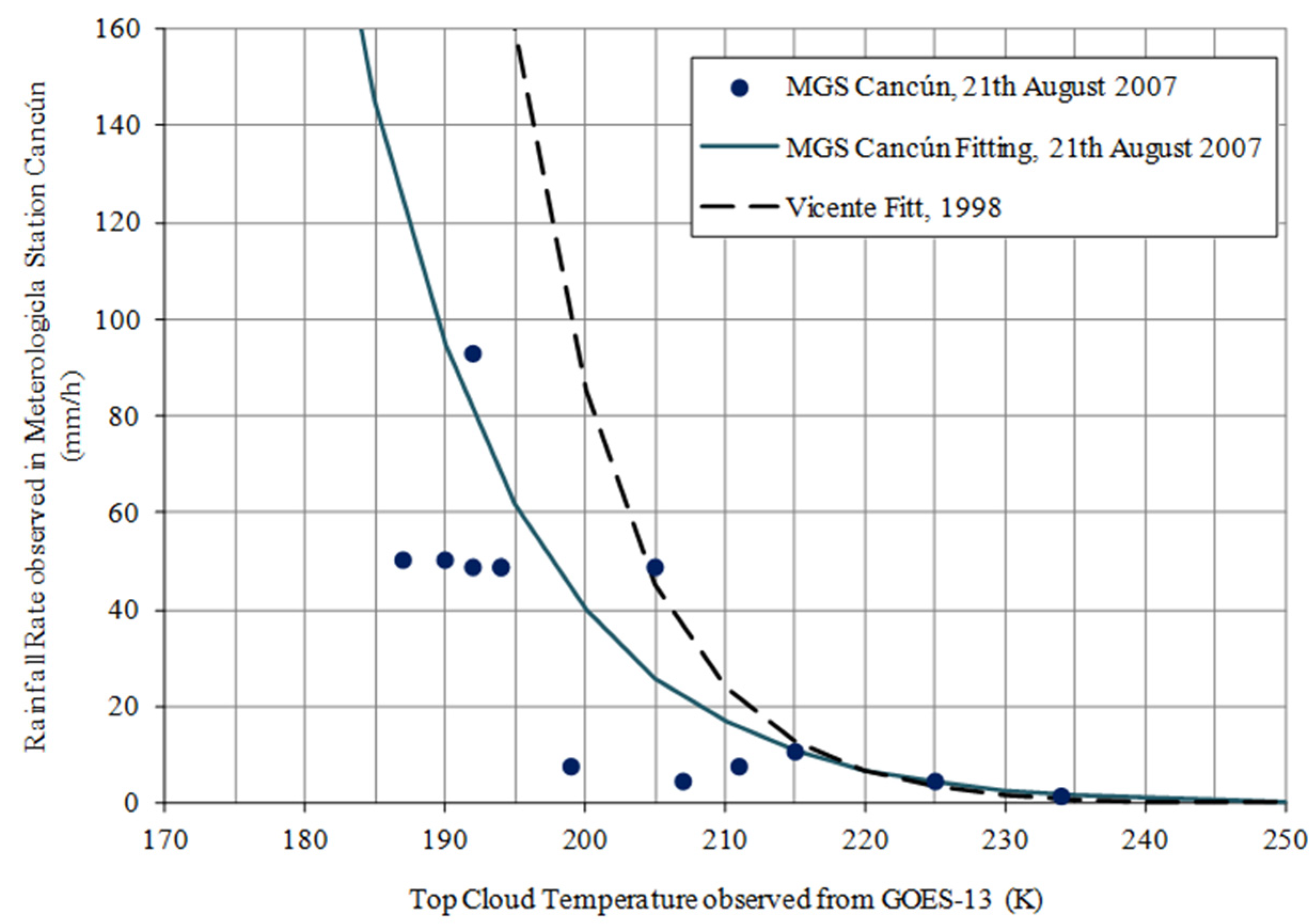
Dean was named as the second major hurricane, cataloged category V in the Saffir–Simpson scale, of the top 20 major hurricanes in Mexico, according to records in the years from 1970 to 2007. Dean caused damage of more than 450 million dollars. The strong winds of up to 230 km/h and the rain caused by Hurricane Dean caused 32 deaths. This hurricane hit the Mexican coast twice. The first impact inland was as a hurricane category V on 21 August at 3:00. The eye of the hurricane Dean impacted land with maximum sustained winds of 260 km/h and gusts of 315 km/h. The Hurricane Center was located at 65 km east of Chetumal, Quintana Roo. After causing devastation in Jamaica and other Caribbean islands, Dean reached the Mexican coast near the Caribbean Coast, not far from the Belize border; the hurricane was moving westward at a speed of 32 km/h. Figure 2 compares the values between the rain intensity recorded by MGS Cancun on 21 August 2007, (from 9:40 to 11:10) with the RR value of the satellite image, and with the new auto-estimator setting proposed by Equation (4). It is important to highlight that the original formula proposed by Vicente et al. [19] that limits the rainfall intensity (RR) to 72 mm/h; however, for this case, the maximum intensity recorded was 92.94 mm/h recorded at 10:00 (192 K temperature value). In all cases, the original form of the equation proposed by Vicente et al. [19] is preserved.
3.2. Hurricane Ernesto MGS Alvarado, Veracruz (9 August 2012)
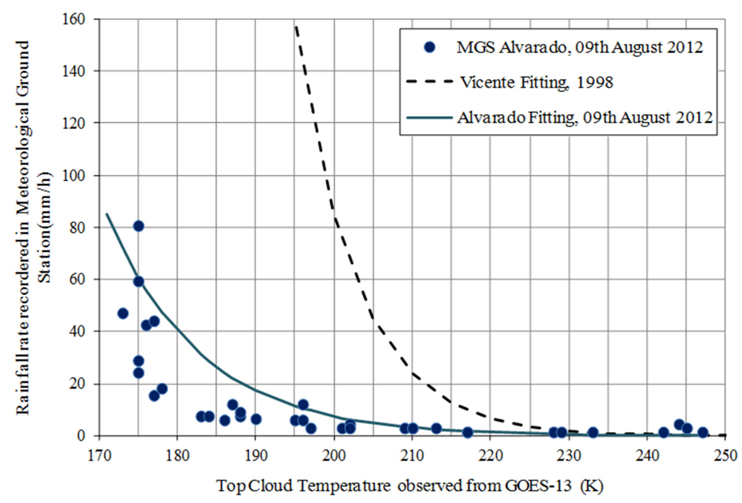
Hurricane Ernesto was formed from a tropical wave developed on 27 July on the African coast; the tropical wave was intensified to a depression storm on 1 August, next to the evolution of this system in Tropical Storm on 2 August, and by 7 August, Ernesto was cataloged as a hurricane category II on the Saffir–Simpson scale. The principal affectation was the heavy rainfall in the states of Yucatán, Quintana Roo, Campeche, Tabasco, and Veracruz. Ernesto made landfall in the south of Quintana Roo, moving west and impacting the Campeche coast. Afterwards, it made a second landfall in Veracruz; this region received more than 300 mm of rain, mainly on the central coast of Veracruz. The state of Veracruz has seven MGS, but just three of them registered the event, and just one registered the maximum rainfall intensity. Alvarado Station received 80.76 mm/h on 9 August 2012 at 14:00 (175 K). The beginning of the measurements was taken from 12:32 an hour before the maximum was registered. For the Hurricane Ernesto, the series of time was greater because rainfall records had a duration of 3 h 10 min. Figure 3 compares the values between the rain intensity recorded by MGS Alvarado on 9 August 2012 (from 06:30 to 16:40) with the RR value of the satellite image, and with the new auto-estimator setting proposed by Equation (5).
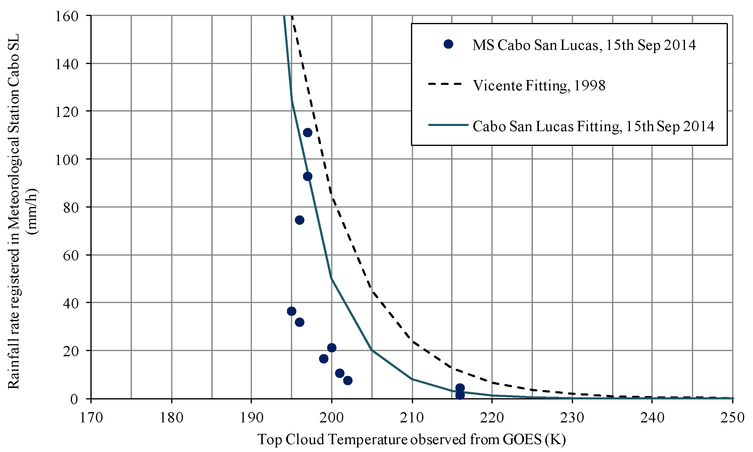
Figure 4 compares the values between the rain intensity recorded by MGS Cabo San Lucas on 15 September 2014 with the RR value of the satellite image of hurricane Odile, and with the new auto-estimator setting proposed by Equation (6).
3.3. Validation
The validation process consists of accepting the estimated RR values from the satellite images (RR–satellite) and comparing them with the RR values obtained from the surface MGS stations (RR–MGS). The validation is made every 10 min when the two RR time series are already matched. A difference is calculated between the measured value in MGS and the RR value of the satellite image. Using an optimization process with the generalized reduced gradient (GRG) nonlinear algorithm of the Excel Solver tool, the difference between the two RR values is minimized.
Other procedures can be used, for example, a procedure based on the maximum likelihood method [29]. Optimization algorithms can be effective for optimizing the training of artificial intelligence models [30,31], multi-layer perceptron neural networks [32], and machine learning models [33]. The use of a meta-heuristic technique as a harmonic search was proposed [34]. In this way, new coefficients of Formula (3) are obtained for each hurricane analyzed. It is important to mention that only the alpha and beta coefficients are changed. The exponent (−1.2) of the original formula is preserved so that the new coefficients have a similarity with the original formula and can be compared.
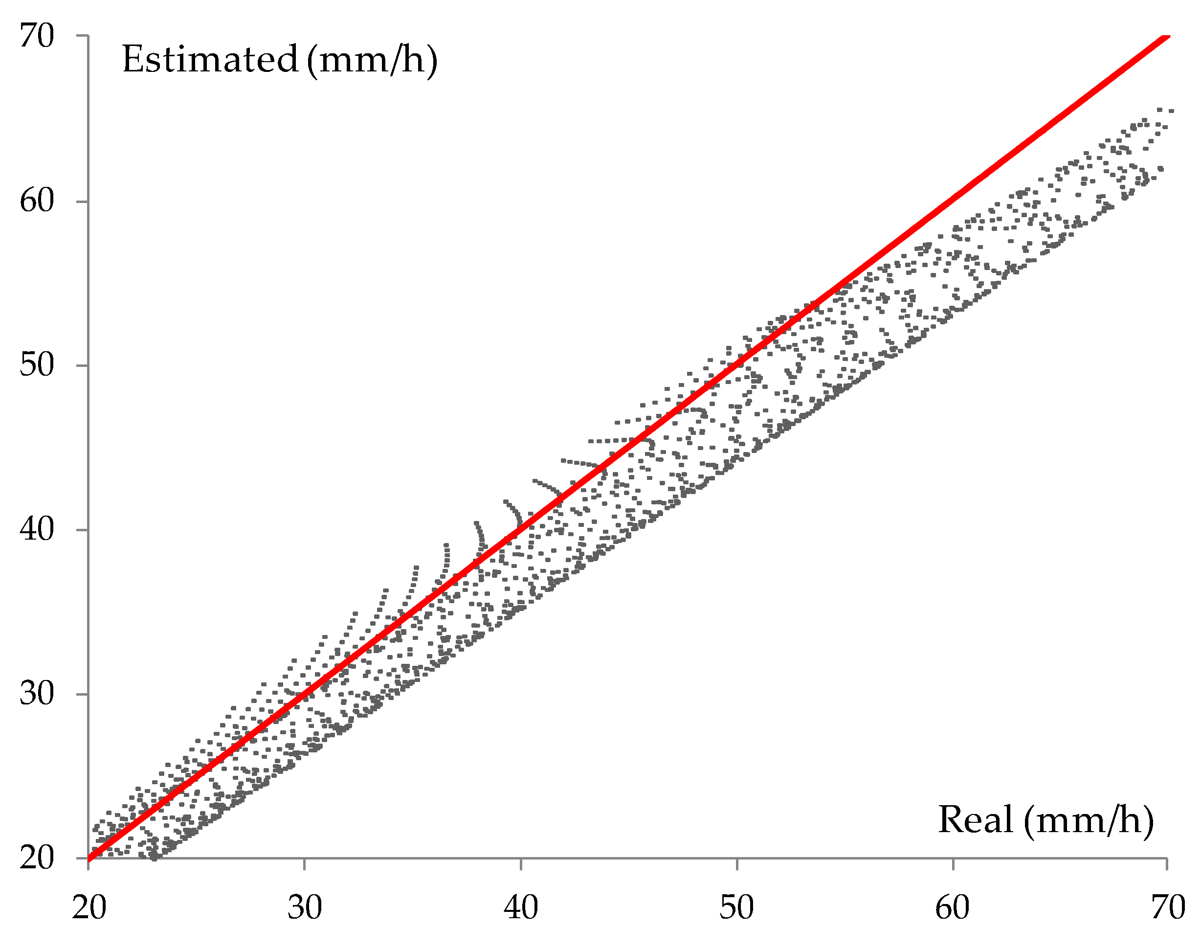
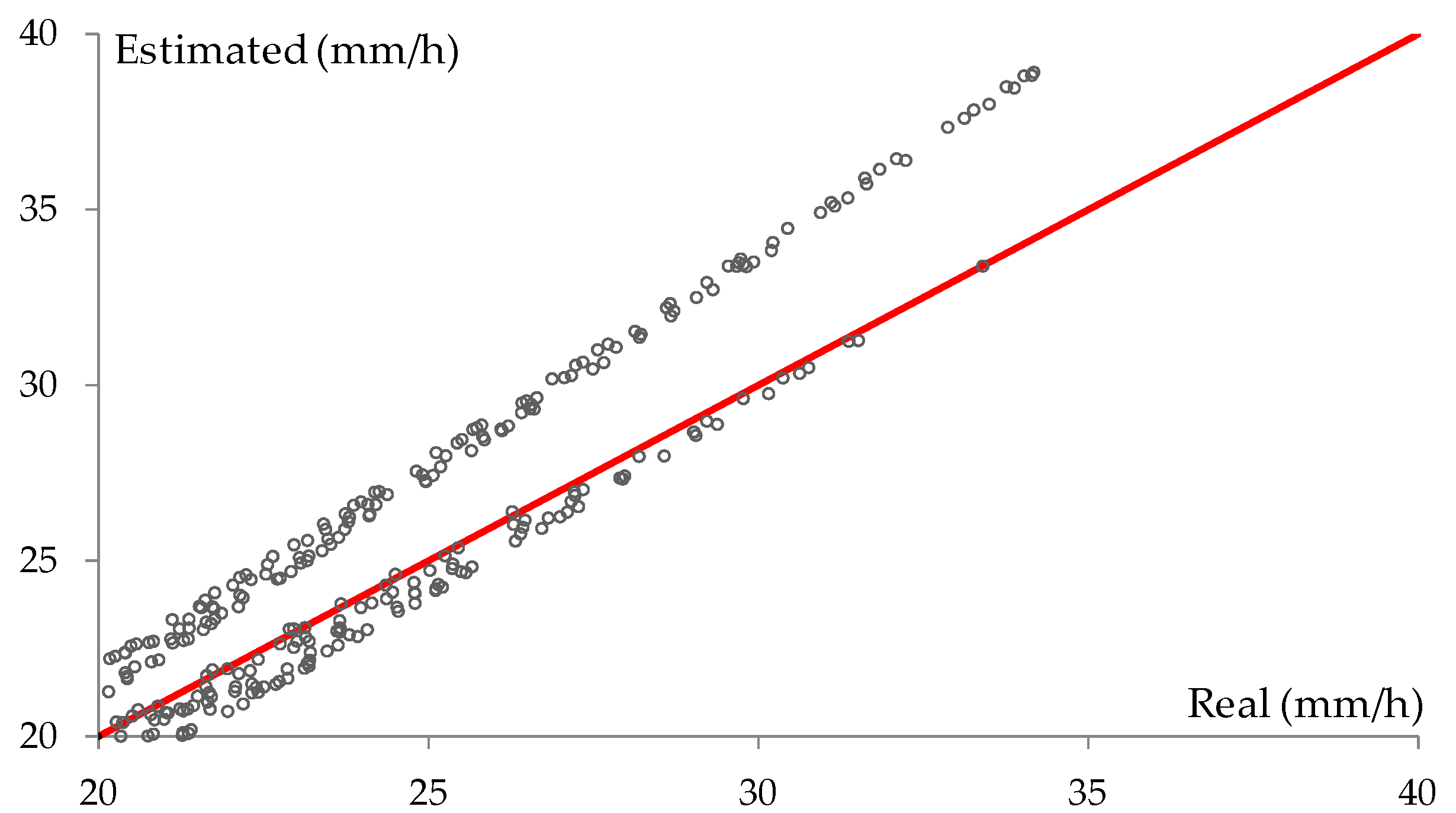
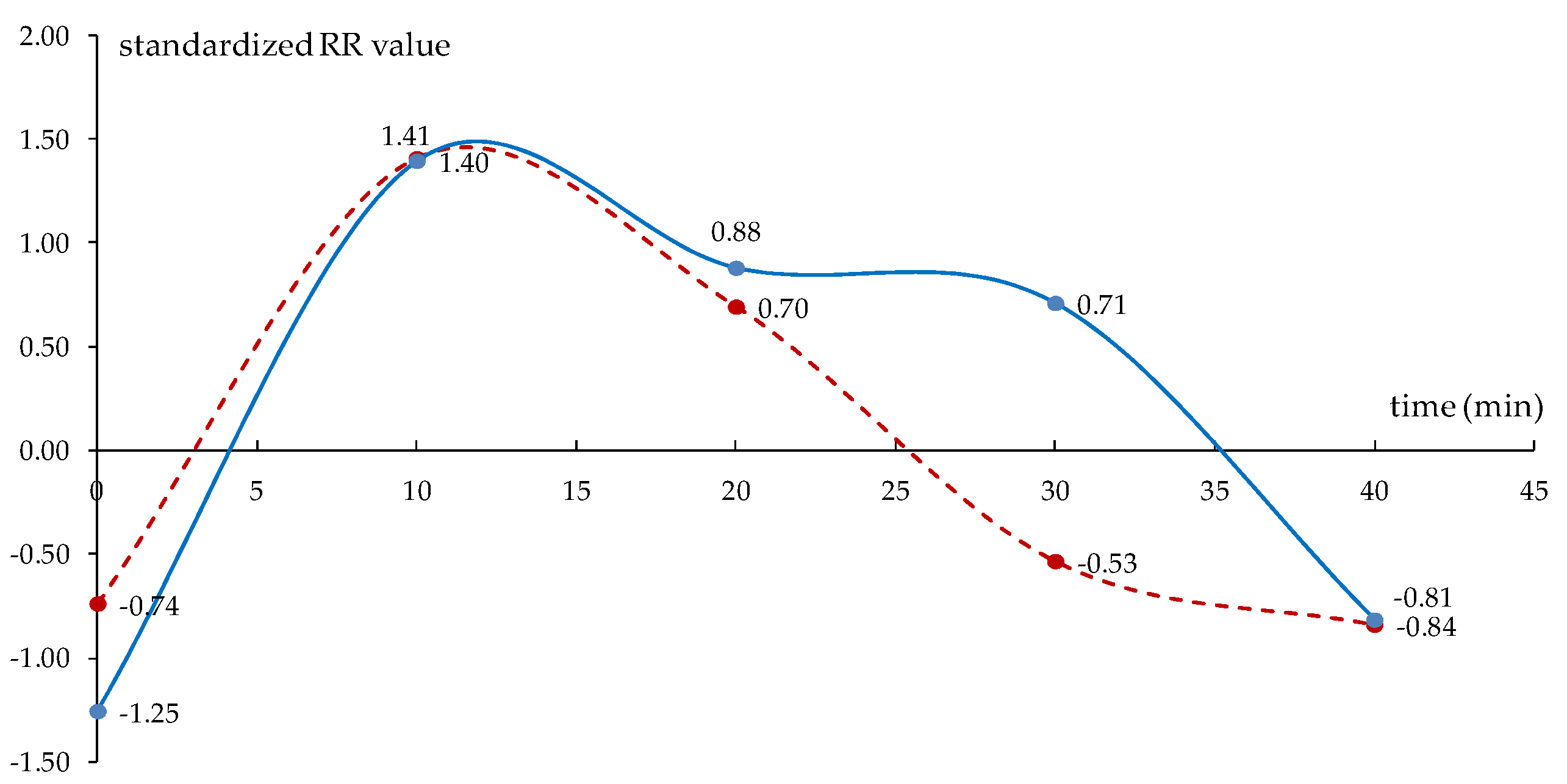
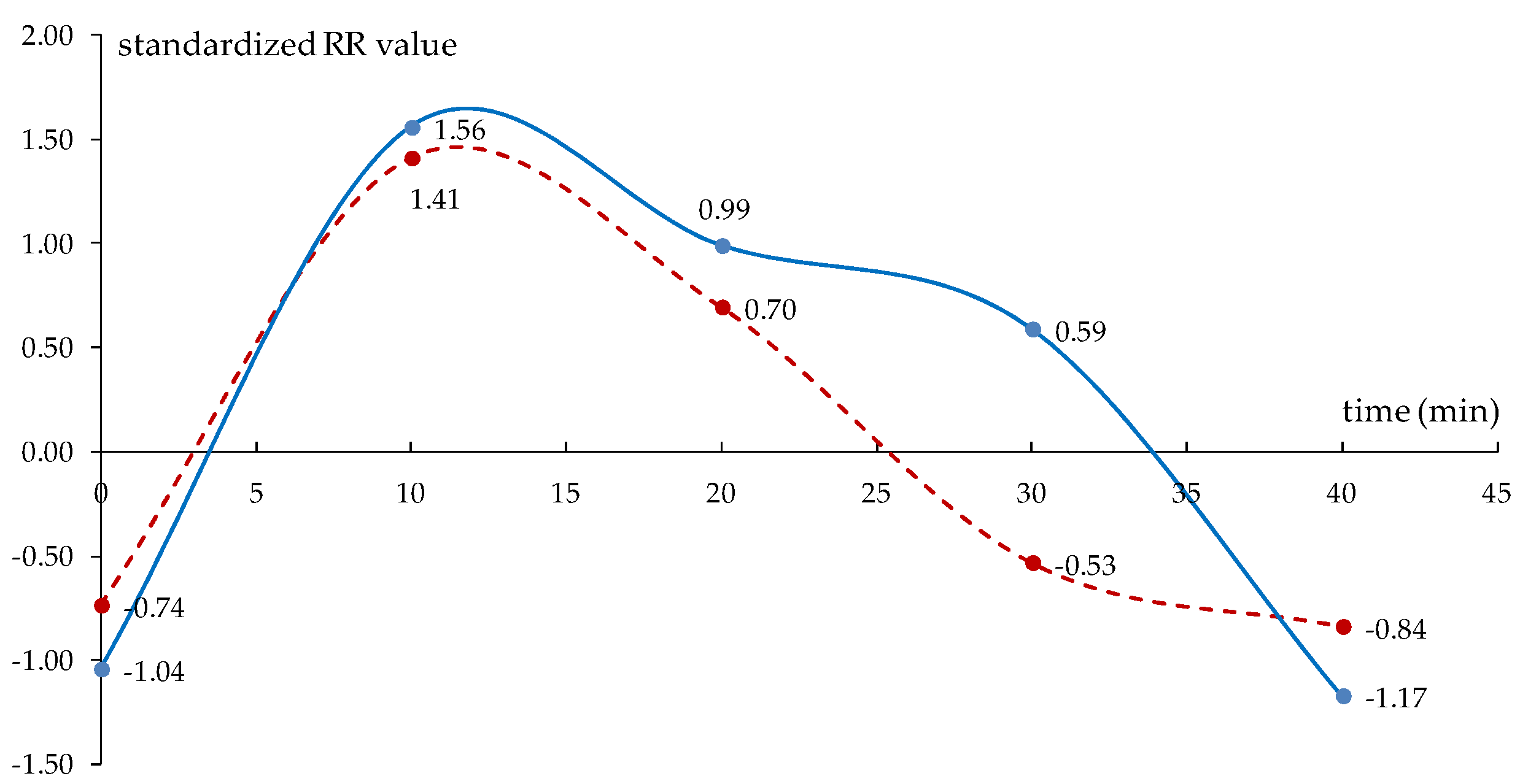
To confirm the new proposed equations, satellite images of the analyzed hurricanes were used at 15-min intervals. With the support of the Sat-Viewer® tool, the intensity of precipitation for each hurricane was calculated. On the other hand, the precipitation intensities were obtained from the MGS stations that recorded the precipitation sheets during the tracks of the hurricanes. Figure 5 and Figure 6 show the results of this procedure as a validation of the proposed equations. Figure 5 shows the validation with Hurricane Odile for days 14 (23:50) to 15 (02:10) of September 2014, compared with the data measured at the Cabo San Lucas station, BCS. According to Equation (6):
Using the same procedure, Figure 6 shows the validation using the data from Hurricane Patricia in October 2015 on the 23rd (22:00) to the 24th (06:30) compared with the data from the Atoyac station, Guerrero. According to Equation (7):
4. Discussion
The auto-estimator technique is typically used to estimate precipitation in deep convective systems collected in 24 h by infrared information [35]. One of the main restrictions of the auto-estimator technique is related to the precipitation from clouds with more cold-tops low, like the nimbostratus, which is ignored if there is no convection present in the environment close. In events of intense precipitation, the contribution of these clouds to the total record of precipitation is small in proportion, but in other cases, it is not negligible. In addition, there are cases of precipitation from clouds stratus in the absence of convection, which occur mainly at extra-tropical latitudes, in which the technique does not either assign precipitation [36]. This finding has important implications for developing the use of the auto-estimator technique in the LAC region, where mostly convective rains can be detected by satellite images. However, the cold cloud-top cannot detect rainy system information, and the radar would have to be used (as commented, countries in the LAC region have poor access to radar data). In the United States, the detection of cloudy areas is carried out with a network of meteorological radars that cover the national territory [37], and cirrus and clusters in the dissipation stage, which do not produce precipitation or are rather low, are filtered in this way. Without the help of radars, the auto-estimator technique confuses these cold cloud tops in areas of cirrus and remains of clusters, with precipitating systems, which was reported by Rozumalski [38]. These results are consistent with those of other studies and suggest that all the remote-sensing products underestimate the rainfall as compared to the rain gauge measurements when evaluated rainfall estimates from ground radar network and satellite algorithms for typhoons at various spatio-temporal scales from 0.04 to 0.25° and hourly to event total accumulation [39].
In the case of hurricanes, the auto-estimator overestimates the precipitations that come from Cumulonimbus clouds that generate large systems such as hurricanes, as shown in Figure 2 and Figure 3. The results of this study show that with no radar data available, the alternative is to change the coefficients in Equation (3) to adjust the RR values to surface precipitation records.
On the other hand, in Equation (3) proposed by Vicente et al. [19], the maximum intensity of rainfall intensity is reached between 195° and 200° K, while in the two cases above, present lower rainfall intensity at those temperatures. In other words, higher intensity occurs at colder temperatures (less than 190° K). This difference in temperature is associated with latitudes near the equator. In Figure 3, it can be observed that the potential fitting for Ernesto values is close to zero or minimum rainfall intensity decreases the potential slope. Precipitation is a well-known phenomenon, and it can make some simplifications, establishing a range of temperatures where rainfall intensity is equal to zero, at the same time getting a fitting in the potential curve with the recorders in the ground. In Figure 2, Hurricane Dean’s fit shows a tendency that corresponds to a power-law curve; according to [19], it is notable that at temperatures colder than 210° K, rainfall intensity increases exponentially. A relevant aspect to consider is the Saffir–Simpson category for hurricanes.
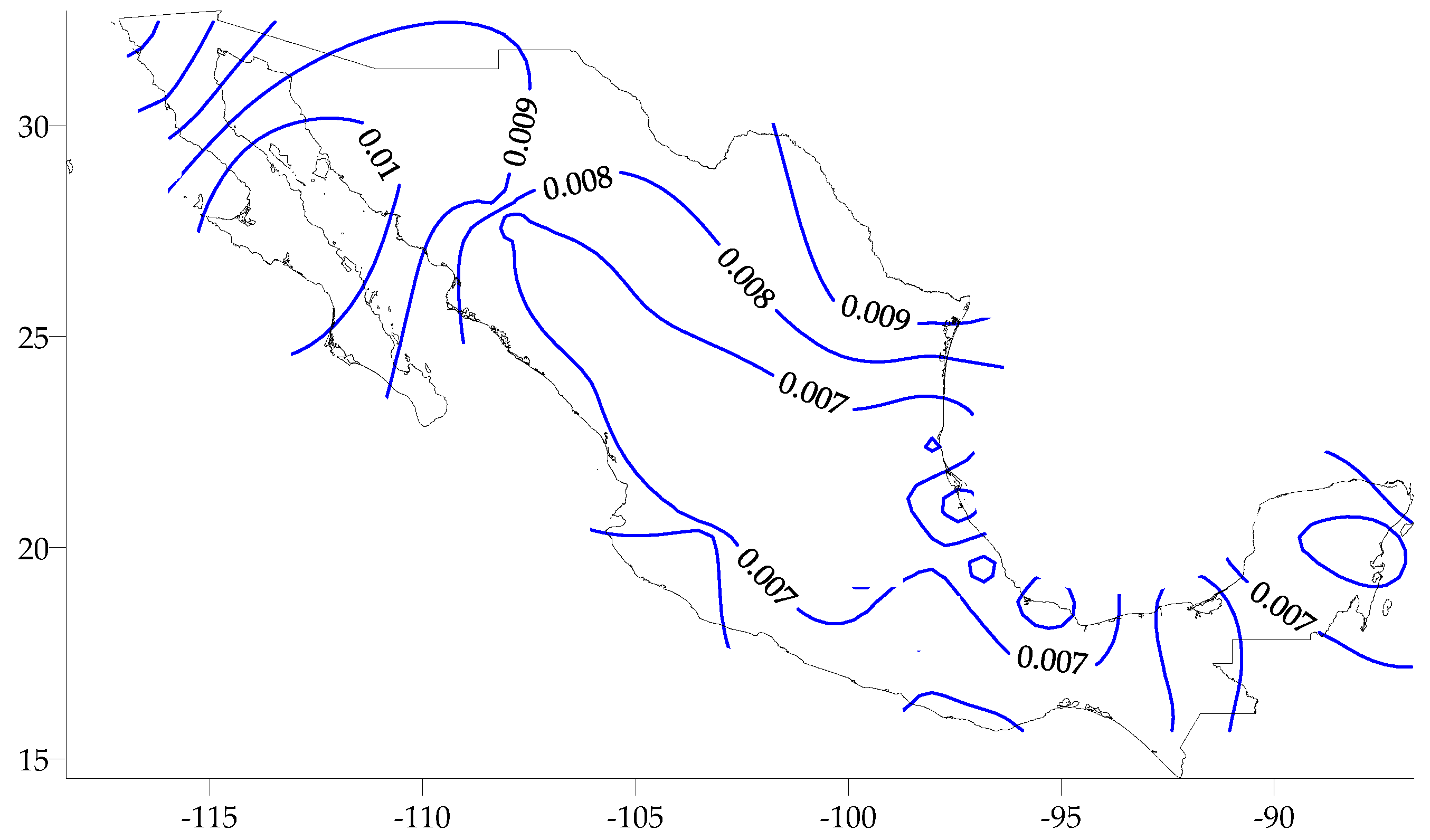
For example, Hurricane Ernesto, categorized as hurricane category II, shows a tendency of coldest temperatures related with minimal rainfall intensity; in contrast, the hurricanes cataloged as major hurricanes, higher than category III, present the highest rainfall intensity in warmer cloud top temperatures, very similar to the relationship demonstrated by Scofield [40]. In this paper, only the results for a few hurricanes are presented. However, 175 storms caused by 14 major hurricanes that have affected Mexico were analyzed. The results show a pattern in the alpha and beta coefficients. Figure 7 and Figure 8 show that there is a spatial pattern in the distribution of the parameter values of the equation proposed by Vicente et al. [19]. This means that the limits of Vincent’s equation must be adjusted for tropical latitudes. Further studies, which take these variables into account, will need to be undertaken the extreme rainfall from hurricanes and the coefficients of auto-estimator. The findings of this study have a number of important implications for the future practice of auto-estimator in the LAC region. Further investigation and experimentation into the Advanced Baseline Imager (ABI) is strongly recommended. The ABI is being developed as the future image on the Geostationary Operational Environmental Satellite GOES-R [41]. The GOES-R rainfall rate algorithm is an infrared-based algorithm calibrated in real-time against passive microwave rain rates [42].
5. Conclusions
For the equation that relates the rainfall intensity with the cloud top temperature, it is important to recall that this equation was developed in the United States of America. The method can be applied in the tropics, but it is important to consider that there are different atmospheric conditions. For example, the highest rainfall intensity that was measured in the hurricanes does not take in count in the original formulation of auto-estimator (limited to 72 mm/h). Since space technology can be accessible for countries that have not developed their own meteorological satellite technology, the sharing information is a relevant hydro-informatics tool for those who see and prognosticate the weather in a wide time–space resolution. The image from GOES provides important information about meso and local scale of hydrometeorological events, which impact the local weather generating severe rainfall, flash floods, and floods. Since we can read this GOES-13 image at almost real-time, it can be read as rainfall intensity in all Mexican territory, providing a beneficial tool, which improves the decision-making in different parts of Mexico. The next step is to develop a connection between the image bright-temperature values to the MGS having the auto-adjusted relationship in real-time. While there are several alternatives to use satellite images, in Mexico, the access is with GOES images. With images from other satellites, the result of applying the technique of auto-estimator will be the same; the only variation would be the resolution of the images.
There are few studies of the coupling of satellite images during the occurrence of hurricanes. Not only is it enough to check their track, but also to match and verify it with surface measurements. Certainly, this work, although it has the limitation of only having used information for Mexico, expects to be the beginning of the verification in the downscaling of the instantaneous precipitation data measured in surface with the satellite data [43].
There is an important opportunity in developing new and innovative techniques and technology based on satellite data adjusted to the tropical latitudes. Further investigations consist of the classification of climatic regions, more specifically, rainfall similarity zones, which include patrons of storms and rainfall intensity in all Mexican territories and the greatest rainfall intensity for each region will be set; as a result, the auto-estimator can be used to monitor rainfall in all states in Mexico where there is no meteorological information available. The hydro-informatics tools developed by www.redciaq.uaq.mx help decision-makers to have a better understanding of hydrometeorological events; they can visualize the possible storms getting close to a specific area in order to act and send help to critical areas. These kinds of hydro-informatics tools give new and reliable information that can support decision-making. At the same time, people can check the weather from home, work, school, and mobile phones. It is important to conduct more investigations and research in this field. Satellite images offer wide time-space coverage, and it is possible to get enough information that can help scientists and researchers to get different values that give understanding and prediction to weather phenomena as a result of climate change.
Author Contributions
Conceptualization, M.M.-R. and A.G.-L.; methodology, M.M.-R.; validation, M.M.-R. and A.G.-L.; formal analysis, A.G.-L.; investigation, M.M.-R.; data curation, M.M.-R.; writing—original draft preparation, M.M.-R.; writing—review and editing, A.G.-L. All authors have read and agree to the published version of the manuscript.
Funding
This work was financially supported by Consejo Nacional de Ciencia y Tecnología (CONACYT). This research received funding from Secretaria de Educacion Publica (SEP-Mexico). Programa para el Desarrollo Profesional Docente (PRODEP) and was supported by the Fund for the Reinforcement of Research UAQ-2018 Research and Postgraduate Division (FOFIUAQ/FIN201911).
Acknowledgments
The authors are grateful to the Risk Management Unit of the UNESCO Regional Office of Science for Latin America and the Caribbean. Special thanks to SMN (Servicio Meterologico Nacional) for the information provided, imagery, and meteorological stations database, to NOAA-NASA GOES Project for sharing data and information, and to Jose Eduardo Hernandez Paulin, Manon Breda, Juan Pablo Molina, Anna Gancarczyk, Claire Fourniret, and Marion Palleschi for their help in data processing. We express our sincere gratitude to Ivonne Cruz and Giselle Galvan Lewis for their detailed style review.
Conflicts of Interest
The authors declare that they have no conflict of interests regarding the publication of this paper.
Appendix A. Wavelet Transformation
Engineers involved in the design of waterworks and the exact natural sciences usually see the time series of hydro-meteorological variables referred to in the time and frequency domain. The origin of the wavelet transformation is due to the need to get the time-frequency disaggregation of a time series. The Fourier transform provides information about which frequencies are present in the time series but does not respond to their exact location in time. The wavelet solution requires a time window of a certain width for all the evaluated frequencies. With the help of the -scale parameter, it is possible to change the width of the window. With the s parameter, called the position-parameter, the location of the series on the time axis is changed [44].
In this way, the wavelet function transforms an input function of t variable into its two-dimensional representation of and s variables. The variable refers to the scale and the variable s represents the time displacement of .
With the hypothesis that a time series can be expressed (or disaggregated) according to its two basic components: the trend represents the main behavior of the RR–MGS, and is the periodic movement of the series in RR–satellite image. The wavelet’s continuous transformation is defined as
denotes the complex conjugate of the function . Equation (A3) can be easily represented as a set of linear, displaced, and invariant filters over time. These filters are described as a convolution of the filtered signal with its response to the pulse :
The steps to follow to find the wavelet transform of a signal are
- It starts with a scale value, e.g., for the wavelet signal; this is placed at the beginning of the data record in t = 0 (see the output in Figure A1).
- The two time series are multiplied together, and the result is integrated over the time-frame. The result of this integration is multiplied by the inverse of the square root of (see the output in Figure A2).
- The wavelet function in the same scale s = 1 is displaced in time to the right in . The procedure of Step (i) is also repeated until the end of the analyzed series is finished (see the output in Figure A3).
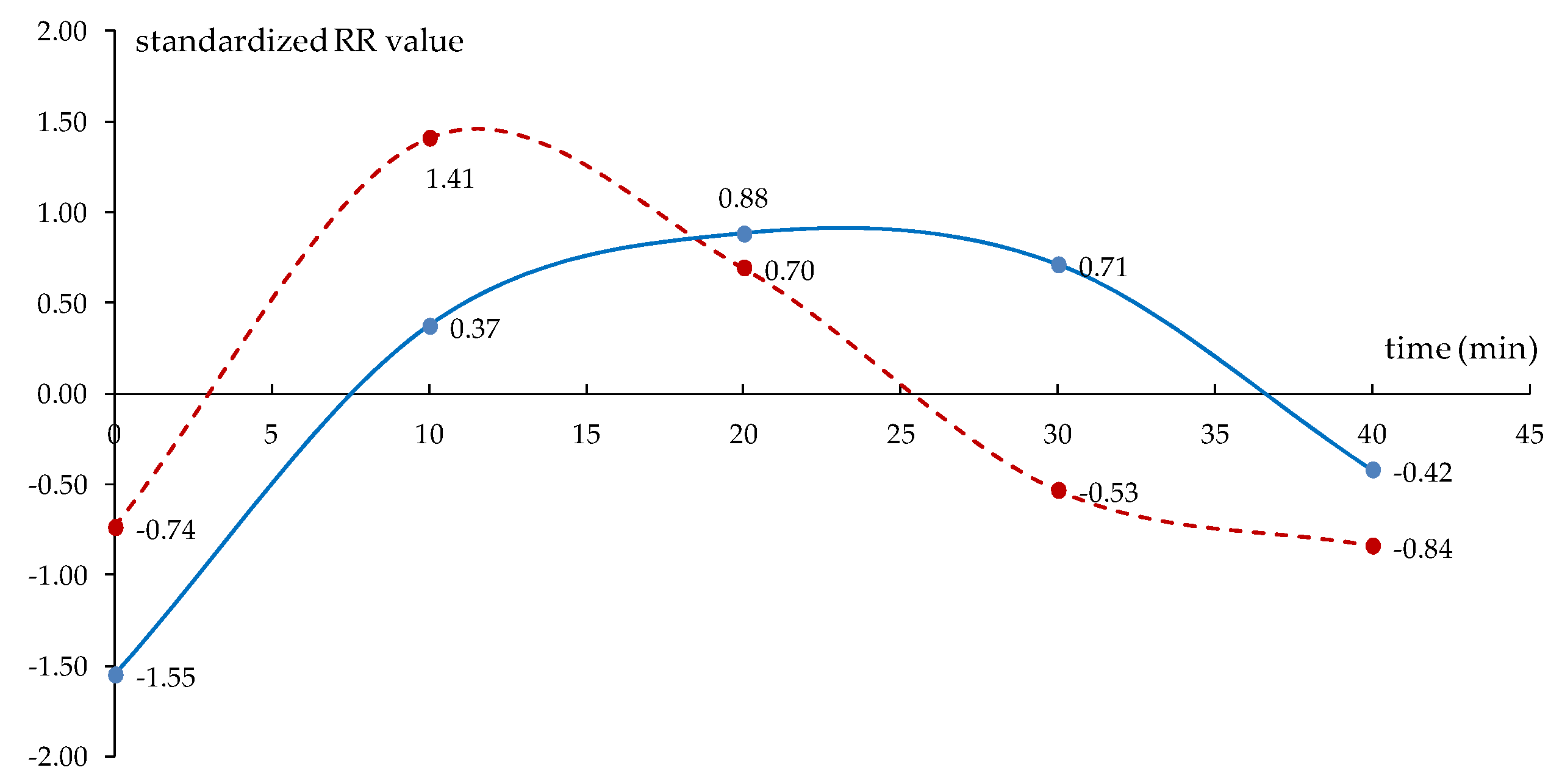
Figure A1.
Temporarily disaggregated series of the RR–MGS Huichapan (red line) and RR–satellite image (blue line) during the Hurricane Manuel (16 Sep 2013), Step (i).
Figure A1.
Temporarily disaggregated series of the RR–MGS Huichapan (red line) and RR–satellite image (blue line) during the Hurricane Manuel (16 Sep 2013), Step (i).

Figure A2.
Temporarily disaggregated series of the RR–MGS Huichapan (red line) and RR–satellite image (blue line) during the Hurricane Manuel (16 Sep 2013), Step (ii).
Figure A2.
Temporarily disaggregated series of the RR–MGS Huichapan (red line) and RR–satellite image (blue line) during the Hurricane Manuel (16 Sep 2013), Step (ii).

Figure A3.
Temporarily disaggregated series of the RR–MGS Huichapan (red line) and RR–satellite image (blue line) during the Hurricane Manuel (16 Sep 2013), final step.
Figure A3.
Temporarily disaggregated series of the RR–MGS Huichapan (red line) and RR–satellite image (blue line) during the Hurricane Manuel (16 Sep 2013), final step.

References
- Berne, A.; Uijlenhoet, R. Path-averaged rainfall estimation using microwave links: Uncertainty due to spatial rainfall variability. Geophys. Res. Lett. 2007, 34. [Google Scholar] [CrossRef] [Green Version]
- Karabatić, A.; Weber, R.; Haiden, T. Near real-time estimation of tropospheric water vapour content from ground based GNSS data and its potential contribution to weather now-casting in Austria. Adv. Space Res. 2011, 47, 1691–1703. [Google Scholar] [CrossRef]
- Menzel, W.; Tobin, D.; Revercomb, H. Infrared Remote Sensing with Meteorological Satellites. Cross Section Data 2016, 65, 193–264. [Google Scholar] [CrossRef]
- Hanssen, R.F. High-Resolution Water Vapor Mapping from Interferometric Radar Measurements. Science 1999, 283, 1297–1299. [Google Scholar] [CrossRef] [PubMed] [Green Version]
- Kidd, C.; Kniveton, D.; Todd, M.C.; Bellerby, T. Satellite Rainfall Estimation Using Combined Passive Microwave and Infrared Algorithms. J. Hydrometeorol. 2003, 4, 1088–1104. [Google Scholar] [CrossRef]
- Kidder, S.Q.; Haar, T.V. Observing Weather from Space. Science 2010, 327, 1085–1086. [Google Scholar] [CrossRef]
- Lopez, V.; Napolitano, F.; Russo, F. Calibration of a rainfall-runoff model using radar and raingauge data. Adv. Geosci. 2005, 2, 41–46. [Google Scholar] [CrossRef] [Green Version]
- Sapiano, M.R.P.; Arkin, P. An Intercomparison and Validation of High-Resolution Satellite Precipitation Estimates with 3-Hourly Gauge Data. J. Hydrometeorol. 2009, 10, 149–166. [Google Scholar] [CrossRef]
- Tang, L.; Tian, Y.; Lin, X. Validation of precipitation retrievals over land from satellite-based passive microwave sensors. J. Geophys. Res. Atmos. 2014, 119, 4546–4567. [Google Scholar] [CrossRef]
- Zabolotskikh, E.; Chapron, B. Validation of the New Algorithm for Rain Rate Retrieval from AMSR2 Data Using TMI Rain Rate Product. Adv. Meteorol. 2015, 2015, 1–12. [Google Scholar] [CrossRef]
- Kestwal, M.C.; Garia, L.S.; Joshi, S. Prediction of Rain Attenuation and Impact of Rain in Wave Propagation at Microwave Frequency for Tropical Region (Uttarakhand, India). Int. J. Microw. Sci. Technol. 2014, 2014, 1–6. [Google Scholar] [CrossRef] [Green Version]
- Mishra, A.K. A New Technique to Estimate Precipitation at Fine Scale Using Multifrequency Satellite Observations Over Indian Land and Oceanic Regions. IEEE Trans. Geosci. Remote. Sens. 2013, 51, 4349–4358. [Google Scholar] [CrossRef]
- Kalinga, O.A.; Gan, T.Y. Estimation of rainfall from infrared-microwave satellite data for basin-scale hydrologic modelling. Hydrol. Process. 2010. [Google Scholar] [CrossRef]
- De Coning, E. Optimizing Satellite-Based Precipitation Estimation for Nowcasting of Rainfall and Flash Flood Events over the South African Domain. Remote. Sens. 2013, 5, 5702–5724. [Google Scholar] [CrossRef] [Green Version]
- Hull, B.V.; Mahani, S.; Autonès, F.; Mecikalski, J.R.; Rabin, R. Infrared satellite rainfall monitoring: Relationships between cloud towers, rainfall intensity, and lightning. Int. J. Water 2014, 8, 343. [Google Scholar] [CrossRef]
- Scofield, R.A.; Kuligowski, R. Status and Outlook of Operational Satellite Precipitation Algorithms for Extreme-Precipitation Events. Weather. Forecast. 2003, 18, 1037–1051. [Google Scholar] [CrossRef] [Green Version]
- Conway, E. The Maryland Space Grant Consortium. In An Introduction to Satellite Image Interpretation; The John Hopkins University Press: Baltimore, MD, USA, 1997; ISBN 0-8018-5576-4. [Google Scholar]
- Kidd, C.; Levizzani, V. Status of satellite precipitation retrievals. Hydrol. Earth Syst. Sci. 2011, 15, 1109–1116. [Google Scholar] [CrossRef] [Green Version]
- Vicente, G.A.; Scofield, R.A.; Menzel, W.P. The Operational GOES Infrared Rainfall Estimation Technique. Bull. Am. Meteorol. Soc. 1998, 79, 1883–1898. [Google Scholar] [CrossRef]
- Tahir, W.; Abu Bakar, S.; Bárdossy, A.; Maznorizan, M. Use of geostationary meteorological satellite images in convective rain estimation for flash-flood forecasting. J. Hydrol. 2008, 356, 283–298. [Google Scholar] [CrossRef]
- Harmening, C.; Neuner, H. A spatio-temporal deformation model for laser scanning point clouds. J. Geod. 2020, 94, 26. [Google Scholar] [CrossRef] [Green Version]
- Benabadji, N.; Hassini, A.; Belbachir, A. Hardware and Software Considerations to Use NOAA Images. Rev. Energ. Ren. 2004, 7, 1–11. [Google Scholar]
- Putra, R.M.; Kurniawan, A.; Rangga, I.A.; Ryan, M.; Endarwin; Luthfi, A. An Evaluation Graph of Hourly Rainfall Estimation in Malang. IOP Conf. Ser. Earth Environ. Sci. 2019, 303. [Google Scholar] [CrossRef]
- Carbajal, M.; Yarlequé, C.; Posadas, A.; Silvestre, E.; Mejía, A.; Quiroz, R. Wavelet daily rainfall data-gap filling using a Wavelet transform-based methodology. Rev. Peru. Geo-Atmosférica 2010, 88, 76–88. [Google Scholar]
- Raje, D.; Mujumdar, P.P. A comparison of three methods for downscaling daily precipitation in the Punjab region. Hydrol. Process. 2011, 25, 3575–3589. [Google Scholar] [CrossRef]
- Goyal, M.K.; Ojha, C.S.P. Evaluation of linear regression methods as downscaling tools in temperature projections over the Pichola Lake Basin in India. Hydrol. Process. 2010, 25, 1453–1465. [Google Scholar] [CrossRef]
- Meusburger, K.; Steel, A.; Panagos, P.; Montanarella, L.; Alewell, C. Spatial and temporal variability of rainfall erosivity factor for Switzerland. Hydrol. Earth Syst. Sci. 2012, 16, 167–177. [Google Scholar] [CrossRef] [Green Version]
- Gutierrez-Lopez, A.; Trejo, M.F.; Gonzalez, N.I.A.; Prado, F.B. Análisis de la variabilidad espacial en la precipitación en la zona metropolitana de Querétaro empleando ecuaciones de anisotropía. Investigaciones Geográficas 2019. [Google Scholar] [CrossRef]
- Escalante-Sandoval, C. Application of bivariate extreme value distribution to flood frequency analysis: A case study of Northwestern Mexico. Nat. Hazards 2006, 42, 37–46. [Google Scholar] [CrossRef]
- Moazenzadeh, R.; Mohammadi, B.; Shamshirband, S.; Ahmadi, M. Coupling a firefly algorithm with support vector regression to predict evaporation in northern Iran. Eng. Appl. Comput. Fluid Mech. 2018, 12, 584–597. [Google Scholar] [CrossRef] [Green Version]
- Fotovatikhah, F.; Herrera, M.; Shamshirband, S.; Ahmadi, M.; Ardabili, S.F.; Piran, J. Survey of computational intelligence as basis to big flood management: Challenges, research directions and future work. Eng. Appl. Comput. Fluid Mech. 2018, 12, 411–437. [Google Scholar] [CrossRef] [Green Version]
- Ghorbani, M.A.; Kazempour, R.; Ahmadi, M.; Shamshirband, S.; Ghazvinei, P.T. Forecasting pan evaporation with an integrated artificial neural network quantum-behaved particle swarm optimization model: A case study in Talesh, Northern Iran. Eng. Appl. Comput. Fluid Mech. 2018, 12, 724–737. [Google Scholar] [CrossRef]
- Shamshirband, S.; Hashemi, S.; Salimi, H.; Samadianfard, S.; Asadi, E.; Shadkani, S.; Kargar, K.; Mosavi, A.; Nabipour, N.; Chau, K.-W. Predicting Standardized Streamflow index for hydrological drought using machine learning models. Eng. Appl. Comput. Fluid Mech. 2020, 14, 339–350. [Google Scholar] [CrossRef]
- Molina-Aguilar, J.P.; Gutierrez-Lopez, A.; Raynal-Villaseñor, J.A.; Garcia-Valenzuela, L.G. Optimization of Parameters in the Generalized Extreme-Value Distribution Type 1 for Three Populations Using Harmonic Search. Atmosphere 2019, 10, 257. [Google Scholar] [CrossRef] [Green Version]
- Xu, W.; Adler, R.F.; Wang, N.-Y. Combining Satellite Infrared and Lightning Information to Estimate Warm-Season Convective and Stratiform Rainfall. J. Appl. Meteorol. Clim. 2014, 53, 180–199. [Google Scholar] [CrossRef]
- Hobouchian, M.; García, Y.; Barrera, D.; Vila, D.; Salio, P. Validación de la estimación de precipitación por satélite aplicando la técnica hidroestimador. Meteorologica 2017, 42, 19–37. [Google Scholar]
- Scofield, R.A. Comments on “A Quantitative Assessment of the NESDIS Auto-Estimator”. Weather. Forecast. 2001, 16, 277–278. [Google Scholar] [CrossRef]
- Rozumalski, R.A. A Quantitative Assessment of the NESDIS Auto-Estimator. Weather. Forecast. 2000, 15, 397–415. [Google Scholar] [CrossRef]
- Chen, S.; Hong, Y.; Cao, Q.; Kirstetter, P.-E.; Yong, B.; Qi, Y.; Zhang, J.; Howard, K.; Hu, J.; Wang, J. Performance evaluation of radar and satellite rainfalls for Typhoon Morakot over Taiwan: Are remote-sensing products ready for gauge denial scenario of extreme events? J. Hydrol. 2013, 506, 4–13. [Google Scholar] [CrossRef]
- Scofield, R.A. The NESDIS Operational Convective Precipitation- Estimation Technique. Mon. Weather. Rev. 1987, 115, 1773–1793. [Google Scholar] [CrossRef]
- Schmit, T.J.; Gunshor, M.M.; Menzel, W.P.; Gurka, J.J.; Li, J.; Bachmeier, A.S. INTRODUCING THE NEXT-GENERATION ADVANCED BASELINE IMAGER ON GOES-R. Bull. Am. Meteorol. Soc. 2005, 86, 1079–1096. [Google Scholar] [CrossRef]
- Kuligowski, R.; Yu, H.; Hao, Y.; Zhang, Y. Improvements to the GOES-R Rainfall Rate Algorithm. J. Hydrometeorol. 2016, 17, 1693–1704. [Google Scholar] [CrossRef]
- Homsi, R.; Shiru, M.S.; Shahid, S.; Ismail, T.; Bin Harun, S.; Al-Ansari, N.; Chau, K.-W.; Yaseen, Z.M. Precipitation projection using a CMIP5 GCM ensemble model: A regional investigation of Syria. Eng. Appl. Comput. Fluid Mech. 2019, 14, 90–106. [Google Scholar] [CrossRef]
- Medina, L. Analisis de tecnicas Wavelet para el Desarrollo de Compresores de Audio; Universidad EAFIT: Medellin, Colombia, 2017; p. 100. [Google Scholar]
Figure 1.
Extraction of the brightness temperature value of the pixels, using the Sat-Viewer®.

Figure 2.
The relationship (R2 = 0.55) between rainfall, the intensity from MGS Cancun 21 August 2007, and temperature of cloud top from the satellite image on the same date of Hurricane Dean.
Figure 2.
The relationship (R2 = 0.55) between rainfall, the intensity from MGS Cancun 21 August 2007, and temperature of cloud top from the satellite image on the same date of Hurricane Dean.

Figure 3.
The relationship (R2 = 0.67) between rainfall intensity from MGS Alvarado on 9 August 2012 and the temperature of cloud tops from the satellite image on the same date of Hurricane Ernesto.
Figure 3.
The relationship (R2 = 0.67) between rainfall intensity from MGS Alvarado on 9 August 2012 and the temperature of cloud tops from the satellite image on the same date of Hurricane Ernesto.

Figure 4.
The relationship (R2 = 0.57) between rainfall intensity from MGS Cabo San Lucas on 15 September 2014 and the temperature of cloud tops from the satellite image at the same date of Hurricane Odile.
Figure 4.
The relationship (R2 = 0.57) between rainfall intensity from MGS Cabo San Lucas on 15 September 2014 and the temperature of cloud tops from the satellite image at the same date of Hurricane Odile.

Figure 5.
Validation of the methodology using data from Hurricane Odile, 14 (23:50) to 15 (02:10) September 2014 at MGS Cabo San Lucas, BCS. (R2 = 0.9387).
Figure 5.
Validation of the methodology using data from Hurricane Odile, 14 (23:50) to 15 (02:10) September 2014 at MGS Cabo San Lucas, BCS. (R2 = 0.9387).

Figure 6.
Validation of the methodology using data from Hurricane Patricia, 23 (22:00) to 24 (06:30) October 2015, in the MGS Atoyac, Guerrero. (R2 = 0.9605).
Figure 6.
Validation of the methodology using data from Hurricane Patricia, 23 (22:00) to 24 (06:30) October 2015, in the MGS Atoyac, Guerrero. (R2 = 0.9605).

Figure 7.
Spatial distribution of alfa parameter of Equation (3).

Figure 8.
Spatial distribution of beta parameter of Equation (3).


Table 1.
Relation of automatic rain-gauge stations (MGS) and the hurricanes studied.
| MGS Name | H. Patricia 20–24 Oct 2015 | H. Dean 13–27 Aug 2007 | H. Odile 9–18 Sep 2014 | H. Manuel 12–20 Sep 2013 | H. Paul 12–18 Sep 2012 | H. Ernesto 1–10 Aug 2012 |
|---|---|---|---|---|---|---|
| Chinipas | D15 1 | - | D15 | D15 | D15 | - |
| Guachochi | D15 | - | - | - | D15 | - |
| Urique | D15 | - | D15 | D15 | D15 | - |
| Maguarichi | D15 | - | - | D15 | D15 | - |
| Cabo San L | - | - | D15 | D15 | D15 | - |
| Cancun | - | D15 | - | - | - | D15 |
| Alvarado | - | D15 | - | - | - | D15 |
| Atoyac | D15 | D15 | - | D15 | D15 | D15 |
| Huichapan | D15 | - | D15 | D15 | D15 | - |
| Chinatu | D15 | - | D15 | D15 | D15 | - |
| Las Vegas | D15 | - | D15 | D15 | D15 | - |
| Obispo | D15 | - | D15 | D15 | D15 | - |
| San Juan | D15 | - | D15 | - | - | - |
| El Fuerte | - | - | - | D15 | D15 | - |
| Alamos | D15 | - | D15 | D15 | D15 | - |
1 D15, data available every 15 min. - MGS did not record any rain at that site.
© 2020 by the authors. Licensee MDPI, Basel, Switzerland. This article is an open access article distributed under the terms and conditions of the Creative Commons Attribution (CC BY) license (http://creativecommons.org/licenses/by/4.0/).
Share and Cite
MDPI and ACS Style
Meza-Ruiz, M.; Gutierrez-Lopez, A. Goes-13 IR Images for Rainfall Forecasting in Hurricane Storms. Forecasting 2020, 2, 85-101. https://0-doi-org.brum.beds.ac.uk/10.3390/forecast2020005
AMA Style
Meza-Ruiz M, Gutierrez-Lopez A. Goes-13 IR Images for Rainfall Forecasting in Hurricane Storms. Forecasting. 2020; 2(2):85-101. https://0-doi-org.brum.beds.ac.uk/10.3390/forecast2020005
Chicago/Turabian StyleMeza-Ruiz, Marilu, and Alfonso Gutierrez-Lopez. 2020. "Goes-13 IR Images for Rainfall Forecasting in Hurricane Storms" Forecasting 2, no. 2: 85-101. https://0-doi-org.brum.beds.ac.uk/10.3390/forecast2020005