Modeling and Forecasting Medium-Term Electricity Consumption Using Component Estimation Technique

Abstract

The increasing shortage of electricity in Pakistan disturbs almost all sectors of its economy. As, for accurate policy formulation, precise and efficient forecasts of electricity consumption are vital, this paper implements a forecasting procedure based on components estimation technique to forecast medium-term electricity consumption. To this end, the electricity consumption series is divided into two major components: deterministic and stochastic. For the estimation of deterministic component, we use parametric and nonparametric models. The stochastic component is modeled by using four different univariate time series models including parametric AutoRegressive (AR), nonparametric AutoRegressive (NPAR), Smooth Transition AutoRegressive (STAR), and Autoregressive Moving Average (ARMA) models. The proposed methodology was applied to Pakistan electricity consumption data ranging from January 1990 to December 2015. To assess one month ahead post-sample forecasting accuracy, three standard error measures, namely Mean Absolute Error (MAE), Mean Absolute Percentage Error (MAPE), and Root Mean Square Error (RMSE), were calculated. The results show that the proposed component-based estimation procedure is very effective at predicting electricity consumption. Moreover, ARMA models outperform the other models, while NPAR model is competitive. Finally, our forecasting results are comparatively batter then those cited in other works.

1. Introduction

Electricity is a key component for the growth and development of any country’s economy. It is a highly flexible form of energy that practically fuels the performance of each sector of an economy. It is a basic requirement of modern human life, bringing benefits and development in different sectors including healthcare, transportation, industries, mining, broadcasting, etc. [1]. Generally, electricity demand is an indication of the performance of a country’s economy as electricity demand is integrated with all phases of development. Therefore, electricity demand forecast is essential for power system management, scheduling, operations, and capability evaluation of networks. In practice, however, electricity demand forecasting remains challenging for researchers as many factors directly or indirectly influence electricity consumption over the time [2,3,4].

Generally, electricity load or price forecasting is divided into three categories with respect to time scale: short term generally refers to forecasts from a few hours to a few days ahead; medium term is used for forecasting of few weeks to few months ahead; and long-term forecasts generally cover forecasts from a few months to years ahead [5]. Short-term electricity load forecasting is essential for the control and programming of electric power systems and also required by transmission companies when a self-dispatching market is in operation [6]. Medium- and long-term forecasts are also important for energy systems. For example, the medium-term electricity demand forecast is required for electric power system operation and scheduling [7,8,9], whereas the long-term electricity demand forecasting is crucial for capacity scheduling and maintenance planning [10].

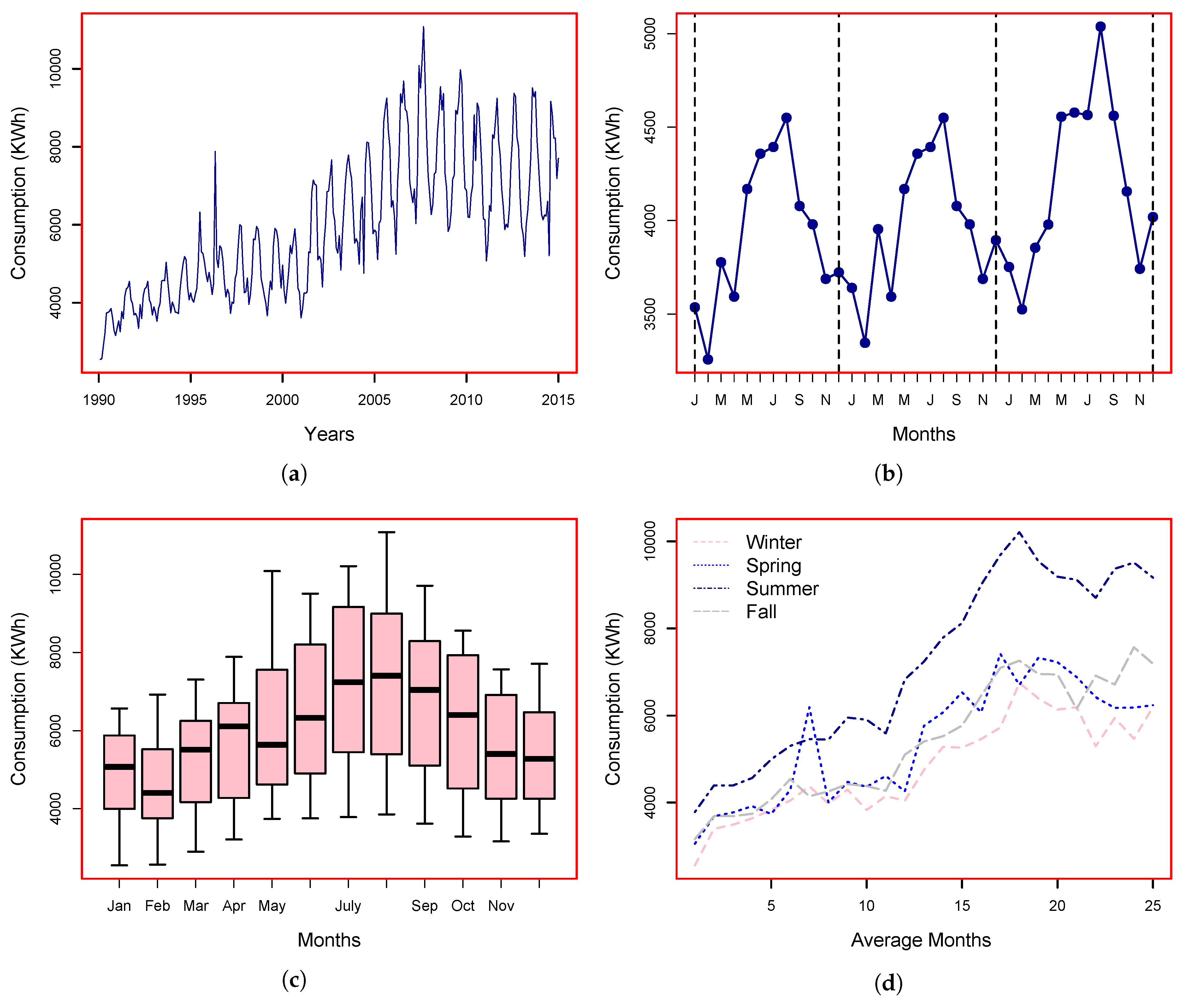
It is well known that electricity demand time series exhibit specific features. The monthly electricity demand time series may have a more or less cyclic behavior and a long-term trend. Electricity consumption is extremely effected by weather and social factors that generally reflect in the demand time series [9,11]. Economic indicators commonly influence the consumption series trend, while climate changes introduce a periodic behavior in the series. The medium-term electricity demand forecasting generally deals with monthly data points, which often include a long-run (trend) component, as well as yearly and seasonal periodicities. For example, Figure 1 depicts Pakistan’s electricity consumption time series for the period January 1990 to December 2016. In the figure, one can see an increasing trend component (Figure 1a), an annual periodicity (Figure 1b), variation of electricity consumption in different months of the year (Figure 1c), and different seasonal effects (Figure 1d).

Previously, many researchers have worked on medium-term electricity demand forecasting that generally ranges from one month to a few months ahead using different methods, including time series, regression, artificial intelligent, genetic algorithm, fuzzy logic, and support vector machine [12,13,14,15,16,17,18,19,20,21,22,23,24,25,26,27,28,29,30,31]. Times series models are easy to implement and have been commonly used for electricity load forecasting in the past. For example, Yasmeen and Sharif [32] used different linear and non-linear time series models, namely AutoRegressive Integrated Moving Average (ARIMA), Seasonal-ARIMA, AutoRegressive conditional heteroscedasticity model (ARCH), and its generalized form, GARCH, to forecast medium-term electricity demand. Electricity demand series often contain non-linearity and, hence, non-linear models can produce better forecasts. For example, Al-Saba and El-Amin [33] forecasted one year ahead electricity consumption for Pakistan using classical time series models, namely Autoregressive (AR) and ARMA models, as well as Artificial Neural Network (ANN). Some authors compared the classical time series and regression models. For example, Abdel-Aal and Al-Garni [34] used multiple regression model and compared it with seasonal and non-seasonal ARIMA models. Economic and weather variables strongly influence electricity demand. To account for these effects, Nawaz et al. [21] studied Pakistan’s annual electricity consumption with the help of economic variables. They forecasted electricity demand up to 10 years ahead using Smooth Transition Auto-Regressive (STAR) model. Many researchers compared time series, regression, and computational intelligence models [16,18]. Electricity load can be effected by temperature. To see this, Ali et al. [35] studied the effect of monthly temperature on electricity demand in Pakistan. The results indicate that there was moderate linear correlation (r = 0.412) between mean temperature and electricity demand. On the other hand, several authors combined the features of two or more than two models and proposed a new model which is often referred as hybrid model [27,30,36,37]. For example, Alamaniotis et al. [13] proposed a hybrid model by combining the features of machine learning tools (kernels) with vector regression model. For medium-term demand forecasting, Ghiassi et al. [38] proposed a hybrid model that combines the neural networks model with expert systems. Several other techniques have been also used to forecast electricity demand [39,40,41]

The purpose of this study was to develop and evaluate model(s) for forecasting medium-term electricity consumption time series. The model(s) are intended to support operational planning and trading decisions. Following the authors of [42,43], in the proposed forecasting methodology, the electricity consumption series is divided into two parts: deterministic and stochastic. Each component is estimated by parametric and nonparametric regression and time series methods. At the end, the forecasts from both components are combined to obtain the final forecast. Thus, the main contribution of this paper is the thorough investigation of the parametric and nonparametric approaches used for medium-term electricity consumption out-of-sample forecasting. Within the framework of the components estimation method, we compare models in terms of forecasting ability considering univariate, parametric, and non-parametric models. Moreover, for the considered models, the significance analysis of the difference in predication accuracy is also conducted.

The rest of the article is organized as follows. Section 2 contains an overview of Pakistan’s electricity sector. Section 3 describes the proposed forecasting framework and information on the models used for forecasting. An application of the proposed forecasting framework is provided in Section 4. Section 5 concludes the study.

2. An Overview of Pakistan Electricity Sector

Pakistan has been facing electricity shortage crisis since its inception. In 1947, Pakistan had the capacity to produce only 60 megawatts (MW) of electricity for its thirty-two million inhabitants. To address the electricity shortage through recognized interventions, the Water and Power Development Authority (WAPDA) was established in 1958. WAPDA built two dams, each with the capacity of about 4478 MW in the late 1970s to overcome the electricity crisis. Pakistan continued facing electricity shortages even in the 1980s even though some haphazard efforts were taken towards improving the situation [44]. With each passing year, the demand for electricity continued rising because of developmental activities, i.e. urbanization, rural electrification, and industrialization [45]. In 1990s, the private sector was given licenses to build new thermal energy plants. It was a strategy shift in terms of the electricity generation mix from hydro to thermal, which increased the cost of electricity generation significantly [46]. Until 2005, the total supply of electricity was surplus to the required demand by approximately 450 MW. During 2007, Pakistan was hit by the worst power crisis in its history. Production fell by 6000 MW, resulting from huge shutdowns all over the country. In 2008, the required electricity demand fell short by 15%, and power outages became more frequent. Furthermore, the existing power stations and electricity distribution networks were also damaged during the 2005 earthquake and 2010 flood [47]. At the same time, the demand for electricity was increasing continuously. For example, from 2001 to 2008, the electricity demand rose by almost 6% per year. In June 2013, the electricity shortage reached 4250 MW per day with demand standing at 16,400 MW per day and generation at 12,150 MW per day [48]. These crisis strongly affected the economic growth and service, despite regular interventions being made to increase electricity production.

Pakistan is a developing country situated in South Asia with a population of over 200 million people. The demand for electricity is increasing exponentially due to an increased demand in both the household and manufacturing sectors. The failure of Pakistan’s power policy over the last few decades has left the country with an acute electricity crisis that increased economic deficit to the country. There are some country specific issues that turn its electricity shortfall into a crisis. These include theft, misuse, and overuse of electricity in the household and industrial sectors; unjustifiably huge line losses; and low institutional capacity, corruption, mismanagement, and political controversies over mega power projects [49].

Pakistan fulfills its electricity requirements by different sources including coil, natural gas, oil, wind, solar, and nuclear [50]. The electricity sector in Pakistan comprises of WAPDA, National Electric Power Regulatory Authority (NEPRA), and a few independent power producers (IPPs). WAPDA and NEPRA are responsible for electric power maintenance, scheduling transmission, and distribution throughout in Pakistan, with the exclusion of Karachi city, which is provided by Karachi Electric Supply Company (KESC). The four main electricity producers in Pakistan includes WAPDA, KESC, IPPs, and Pakistan Atomic Energy Commission (PAEC). The total power generation volume of Pakistan as of 30 June 2015 was 24,823,000 kW, of which thermal was 16,814,000 kW (67.74%), hydro-electric was 71,160,000 kW (28.67%), nuclear was 7,870,000 kW (3.17%), and wind was 106,000 kW (0.43%) [51].

Table 1. Pakistan Electricity: Installed Generation Capacity by different resource (MW) [50].

SOURCE	PRODUCER	2011	2012	2013	2014	2015
	WAPDA Hydel	6516	6516	6733	6902	6902
HYDEL	IPPs Hydel	129	214	214	214	214
	Sub-Total	6645	6730	6947	7116	7116
	% Share Generation	28.47	28.65	29.28	29.99	28.67
	GENCOs with PEPCO	4785	4785	4785	4590	5762
	KESC Own	1821	2381	2359	1951	1874
	IPPs	4288.5	4282	4297	4489	201.5
THERMAL	RPPs	201.5	0	0	0	0
	CPPs/SPPs (KESC)	324	239	203	200	200
	Sub-Total	15,910	15,969	15,941	15,719	16,814
	% Share Generation	%68.16	67.99	67.19	66.25	67.74
	CHASNUPP I-II (NTDC)	650	650	650	650	650
NUCLEAR	KANUPP (NTDC)	137	137	137	137	137
	Sub-Total	787	787	787	787	787
	% Share Generation	3.37	3.35	3.32	3.32	3.17
	Wind P-P (PEPCO)	0	1	50	106	106
WIND	Sub-Total	0	1	50	106	106
	% Share Genration	0	0	0.21	0.45	0.43
	Total Installed Cap	23,342	23,487	23,725	23,728	24,823

describe the installed electricity generating volumes of Pakistan during 2011–2015.

3. Proposed Forecasting Model

The main objective of this study was to forecast one month ahead electricity consumption for Pakistan. Let $C_m$ be electricity consumption for mth month. To account the dynamics of electricity consumption time series, we propose $C_m$ can be modeled as:

$$C_m=D_m+S_m$$

(1)

i.e., the electricity consumption series $C_m$ is divided into two major components: $D_m$, a deterministic component, and $S_m$, a stochastic component. The deterministic component includes trend (log-run) and yearly periodicity. Mathematically, $D_m$ is defined as

$$D_m=T_m+Y_m$$

(2)

where $T_m$ represents the trend (long-term) and $Y_m$ represents the yearly periodicity component. On the other hand, $S_m$ is a stochastic component (residuals), which defines the short-run dynamics. For the estimation of deterministic component $D_m$, both parametric and nonparametric approaches are used. Parametric approaches include polynomial regression, whereas nonparametric ones include regression splines technique. For stochastic component estimation, this work considers four different univariate time series models: AutoRegressive (AR) model, Nonparametric AutoRegressive (NPAR) model, Smooth Transition AutoRegressive (STAR), and AutoRegressive Moving Average (ARMA) model. Hence, combining deterministic and stochastic models leads to eight different possible combinations for comparison purposes $(2^{D_m}\times 4^{S_m}=8)$.

3.1. Modeling the Deterministic Component

3.1.1. Parametric Case

This section describe the estimation of deterministic component using parametric regression method. The response variable $C_m$ is modeled parametrically by estimating the trend (long-run) component $T_m$ using cubic polynomial regression for time m and yearly periodicity is described by dummies as

$$Y_m=\sum _{i=1}^{12}{\varphi }_i{I}_{i,m}$$

with $I_{i,m}=1$ if m refers to the ith month of the year and 0 otherwise. All regression coefficients related to these components are estimated by using Ordinary Least Square (OLS) method. Once all regression coefficients are obtained, the estimated equation is given by

$${\widehat{D}}_m=\widehat{{\varphi }_0}{T}_m+\widehat{{\varphi }_1}{T}_m^2+\widehat{{\varphi }_2}{T}_m^3+\sum _{i=3}^{14}\widehat{{\varphi }_i}{I}_{i,m}$$

(3)

In the past, many researchers used this method for trend and yearly cycle components estimation [52,53,54,55].

3.1.2. Nonparametric Case

In the literature, many authors captured trend and yearly cycle in a time series using nonparametric regression methods. For example, some authors used smoothing spline [43,56,57], kernel regression [58,59,60,61], and regression spline [43,62]. In our case, the deterministic component can be modeled nonparametrically as follows.

$$D_m=h_1\left(T_m\right)+h_2\left(Y_m\right).$$

(4)

Here, each $h_i$ is a smoothing function of $T_m$ and $Y_m$. For yearly cycles, the smooth function is estimated from the series $1,2,3,\dots ,12,1,2,3,\dots ,12,\dots$, whereas the long-term (trend) $T_m$ is estimated as a function of time m. For the smoothing functions, cubic regression splines are used to estimate the deterministic component. In regression spline approach, the most important selection is the number of knots and their location as they define the smoothness of the approximation. For this issue, we use cross validation (CV) technique. Regression coefficients are estimated by using OLS method and the estimated equation is given by:

$${\widehat{D}}_m=\widehat{h_1}\left(T_m\right)+\widehat{h_2}\left(Y_m\right)$$

(5)

Once the deterministic component is estimated, the residual (stochastic) component can be obtained as:

$$S_m=\left(C_m\right)-{\widehat{T}}_m-{\widehat{Y}}_m$$

(6)

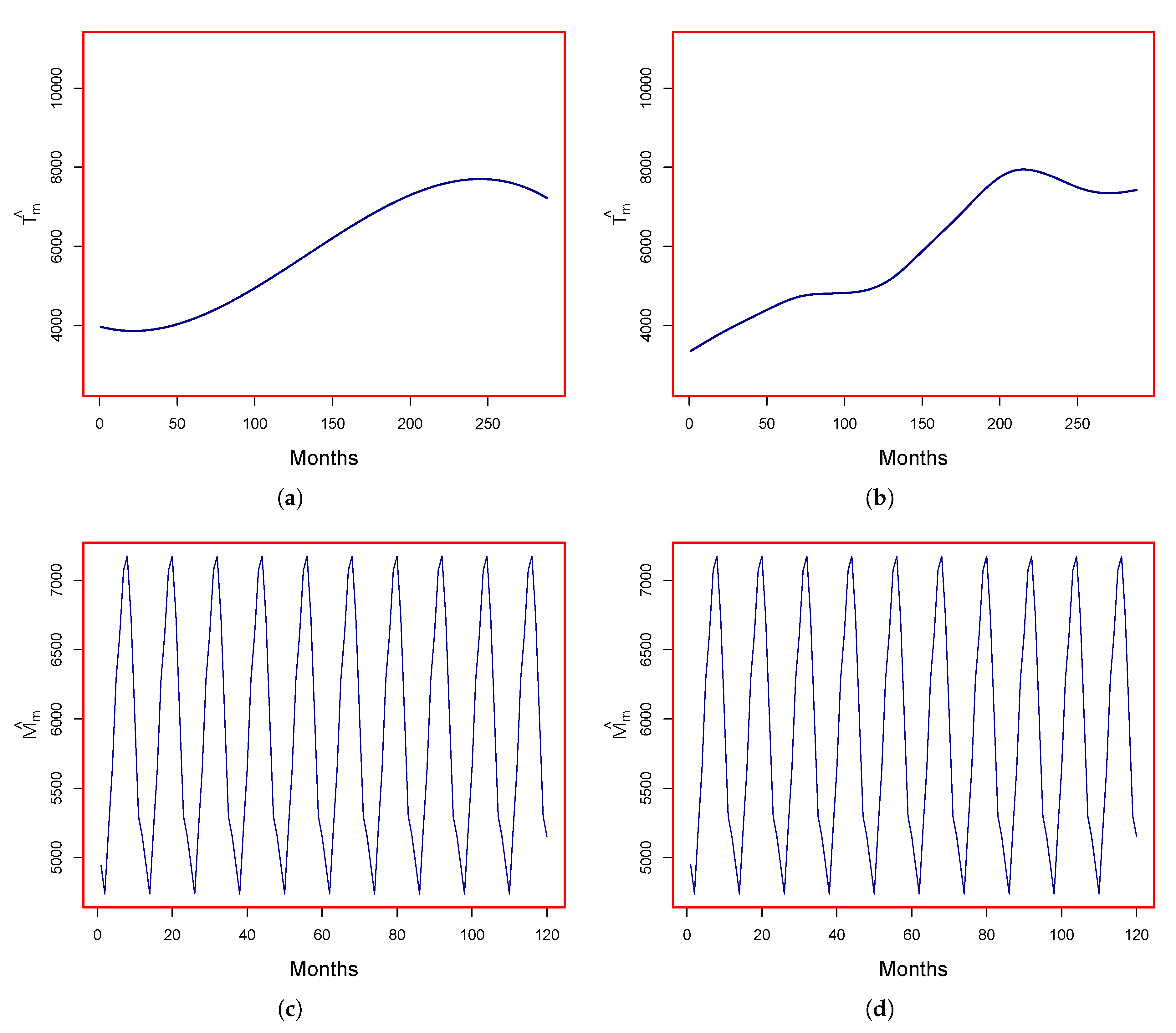
To see the performance graphically of the above-described methods used for estimation of deterministic components $D_m$ (both parametric and nonparametric), the observed electricity consumption and the estimated deterministic component are depicted in Figure 2, with parametric estimation of $D_m$ (Figure 2a) and nonparametric estimation of $D_m$ (Figure 2b). In the figure, it is evident that both models used for the estimation of $D_m$ capture adequately both dynamics, i.e. long trend and yearly seasonality, of electricity consumption series, as the increasing (upward) trend and yearly cycles can be seen clearly in the figure. Using Equation (6), the stochastic (residual) component obtained from both methods are also plotted in Figure 2.

Here, it is worth mentioning that, in general, the stationarity of a time series are inspected using the Augmented Dickey–Fuller (ADF) and Philips–Perron (PP) tests [63,64]. However, several researchers showed that the ADF and PP tests may produce biased and misleading results owing to the possibility of structural breaks in the time series data [65]. Additionally, for the electricity market variables, i.e., prices or demand time series, the unit-root test results are weaker due the presence of periodicities and exceptionally heavy tailed data, which affect the size and power of standard unit-root tests [66,67]. In our case, we did not apply these tests because, once the consumption series is filtered for deterministic component, the stochastic component is always almost stationary.

3.2. Modeling the Stochastic Component

After the estimation of deterministic component using parametric and nonparametric techniques, the remaining part (residuals), considered as stochastic component, is obtained through Equation (6). The residual series obtained from both models are plotted in Figure 3. To model and forecast the stochastic component, this work consider four different univariate time series models: parametric AutoRegressive (AR), nonparametric AutoRegressive (NPAR), Smooth Transition AutoRegressive (STAR), and Autoregressive Moving Average (ARMA) models. Details about these models are given in the following.

3.2.1. AutoRegressive Model

An Autoregressive (AR) model is a widely used model in the time series literature. The AR models describes the response variable linearly dependent on its own past (lag) values and on a stochastic term. The general form of an AR(n) model is given by

$$S_m=\mu +{\alpha }_1{S}_{m-1}+{\alpha }_2{S}_{m-2}+\dots +{\alpha }_n{S}_{m-n}+{ϵ}_m$$

(7)

where $\mu$ indicates the intercept, ${\alpha }_i$$(i=1,2,\dots ,n)$ are parameters of AR(n) model, and ${ϵ}_m$ is a white noise process with mean zero and variance ${\sigma }_{ϵ}^2$. After plotting the ACF and PACF of the series, we concluded that lags 1, 2, and 12 are significant and, hence, are included in the model. In this work, the parameters are estimated using the Maximum Likelihood Estimation (MLE) method.

3.2.2. Nonparametric AutoRegressive Model

The linear AutoRegressive model can be generalized by removing the linearity property. We denote the model by Nonparametric AutoRegressive (NPAR) model. In this case, the relation between the present and past values does not have a particular parametric form and thus accounts for any potential type of nonlinearity in the data. Mathematically, NPAR is given by

$$S_m=h\left(S_{m-1}\right)+h\left(S_{m-2}\right)+\dots +h\left(S_{m-n}\right)+{ϵ}_m$$

(8)

where $h_i$ are smoothing functions describing the relation between each past values and $S_m$. In this work, functions $h_i$ refers to cubic regression spline functions. As done in the parametric case, we used lags 1, 2, and 12 to estimate NPAR. To overcome the curse of dimensionality, which is attributed to the exponential decline of data points within a smoothing window by increasing the dimension of regressors, generally, an additive form is considered that assumes no interactions among the explanatory variables [68].

3.2.3. Smooth Transition AutoRegressive (STAR) Model

The Smooth Transition AutoRegressive (STAR) model is an extension of AR model that allow smooth transition in regime switching models. To control the regime switching process, the STAR model makes use of logistic and exponential functions instead of the indicator function used in threshold AR models. Mathematically, STAR model is defined as

$$S_m={\mathbf{Z}}_{\mathbf{m}}+R_m({\omega }_m,\eta ,\mu ){\mathbf{Z}}_{\mathbf{m}}+{ϵ}_m$$

(9)

where ${\mathbf{Z}}_{\mathbf{m}}=(1,S_{m-2},S_{m-1},\cdots ,S_{m-n})$, $R_m({\omega }_m,\eta ,\mu )$ is the transition function bounded between 0 and 1, and ${\omega }_m$ is a transition variable. The parameter $\eta$ represents the speed and smoothness of transition, while $\mu$ can be interpreted as threshold between two regimes. Finally, ${ϵ}_m$ is a white noise process that is assumed to be normally distributed with mean zero and variance ${\sigma }_{ϵ}^2$. This model is defined as a two-regime switching model, in which the transition function R allows the dynamics of the model to switch between regimes smoothly. A common specification of the generalized version of smooth transition functions is given by

$$R_m(w_m,\eta ,a)={\left\{1+exp\left[\frac{-\eta }{{\sigma }_{{\omega }_m}^k}{\prod }_k{\left({\omega }_m-a_k\right)}^k\right]\right\}}^{-1}$$

(10)

where ${\sigma }_{{\omega }_m}$ is the standard deviation of the transition variable. STAR implements the iterative building strategy described in [69] to identify and estimate STAR model.

3.2.4. AutoRegressive Moving Average Model

Autoregressive Moving Average (ARMA) model not only includes the past lagged values of the variable of interest but also considers the past lags of error term. In our case, the response variable $S_m$ is modeled linearly using its past values as well as past white noise terms, i.e.,

$$S_m=\mu +\left(\sum _{i=1}^r{\alpha }_i{S}_{m-n}\right)+\left(\sum _{j=0}^s{\varphi }_j{ϵ}_{m-s}\right)$$

(11)

where $\mu$ indicates intercept; ${\alpha }_i$$(i=1,2,\dots ,n)$ and ${\varphi }_j$$(j=1,2,\dots ,s)$ are parameters of AR and MA, respectively; and ${ϵ}_m$ is a Gaussian white noise series with mean zero and variance ${\sigma }_{ϵ}^2$. Inspection of the ACF and PACF suggests that, for AR part, lags 1, 2, and 12 are significant, while the first two lags for the MA part. Thus, a constrained ARMA(12,2) where ${\alpha }_3=,\cdots ,={\alpha }_{11}=0$ is fitted to $S_m$ using the MLE method.

Once both components, deterministic and stochastic, are estimated, the final one month ahead forecast is obtained as

$${\widehat{C}}_{m+1}=({\widehat{T}}_{m+1}+{\widehat{Y}}_{m+1}+{\widehat{S}}_{m+1})$$

(12)

4. Out-of-Sample Forecasting

In this study, we used monthly electricity consumption aggregated data of Pakistan. The dataset was obtained from Pakistan Bureau of Statistics (PBS). The monthly series ranges from January 1990 to December 2014 and measured in kilowatt hours (kWh). The whole dataset contains 288 data points, of which data from January 1990 to December 2009 (240 data points) were used for model estimation and from January 2010 to December 2014 (48 data points) for one month ahead out-of-sample forecasts. The monthly electricity consumption series was represented by $C_m$, where $(m=1,2,\dots ,288)$. For the forecasting accuracy, three standard accuracy measures—Mean Absolute Error (MAE), Mean Absolute Percentage Error (MAPE), and Root Mean Square Error (RMSE)—for each model were calculated as follows:

$$MAPE=Mean\left(\frac{|C_m-{\widehat{C}}_m|}{|C_m|}\right)\times 100$$

$$MAE=Mean\left(|C_m-{\widehat{C}}_m|\right)$$

$$RMSE=\sqrt{Mean{(C_m-{\widehat{C}}_m)}^2}$$

where $C_m$ denotes observed series and ${\widehat{C}}_m$ represents forecasted consumption series for mth month. Combining models for the both components, deterministic and stochastic, led us to compare eight different possible combination, namely P-AR, P-NPAR, P-STAR, P-ARMA, NP-AR, NP-NPAR, NP-STAR, and NP-ARMA, where the first letter(s) represents the deterministic part with ‘P’ standing for parametric and ‘NP’ for nonparametric estimation, and the second part used for the stochastic model.

To assess the best combinations of these models, we calculated different accuracy measures and tabulated the results in

Table 2. Model accuracy statistics for one month ahead out-of-sample forecast.

Model	MAPE	MAE	RMSE
P-STAR	5.56	397.99	513.22
P-AR	6.38	454.49	569.74
P-NPAR	6.19	439.79	563.21
P-ARMA	4.84	355.24	467.42
NP-STAR	5.44	402.78	526.67
NP-AR	5.93	435.63	550.41
NP-NPAR	5.18	379.98	492.81
NP-ARMA	4.83	348.31	460.80

. In the table, it is clear that both the ARMA models outperform all the competitors as they produce better results. The MAPE values for P-ARMA and NP-ARMA are 4.84 and 4.83, respectively. The second best model is NP-NPAR for which the MAPE value is 5.18. The MAPE values for all combinations are also plotted in Figure 4 where the superiority of models involving ARMA model can be clearly seen.

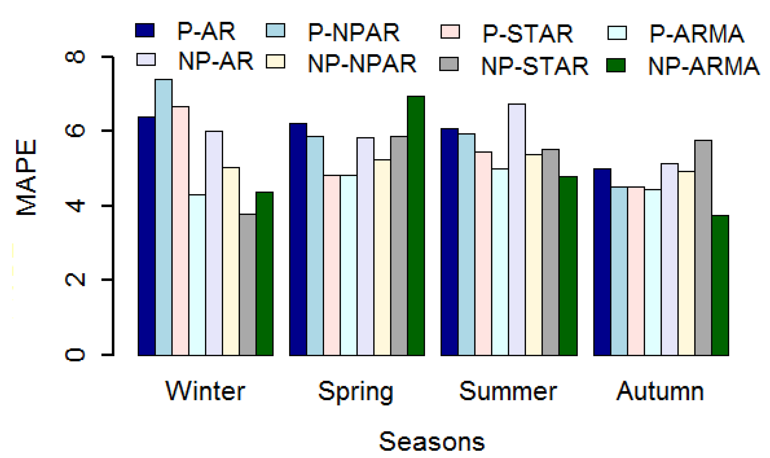
The season-specific errors are listed in

Table 3. One month ahead post-sample forecasts MAPEs with respect to seasons of the year.

Models	Winter	Spring	Summer	Autumn
P-AR	6.38	6.21	6.09	5.00
P-NPAR	7.40	5.86	5.96	4.53
P-STAR	6.66	4.84	5.47	4.50
P-ARMA	4.31	4.84	5.02	4.45
NP-AR	6.03	5.83	6.75	5.14
NP-NPAR	5.05	5.26	5.39	4.92
NP-STAR	3.78	5.86	5.53	5.77
NP-ARMA	4.36	6.96	4.79	3.74

. In the table, we can observe that the season-specific MAPEs are comparatively low in autumn and high in the remaining three seasons. Except in spring, the season-specific MAPE values for P-ARMA and NP-ARMA are considerably lower than those of the other models. The season-specific MAPEs values are also plotted in Figure 5.

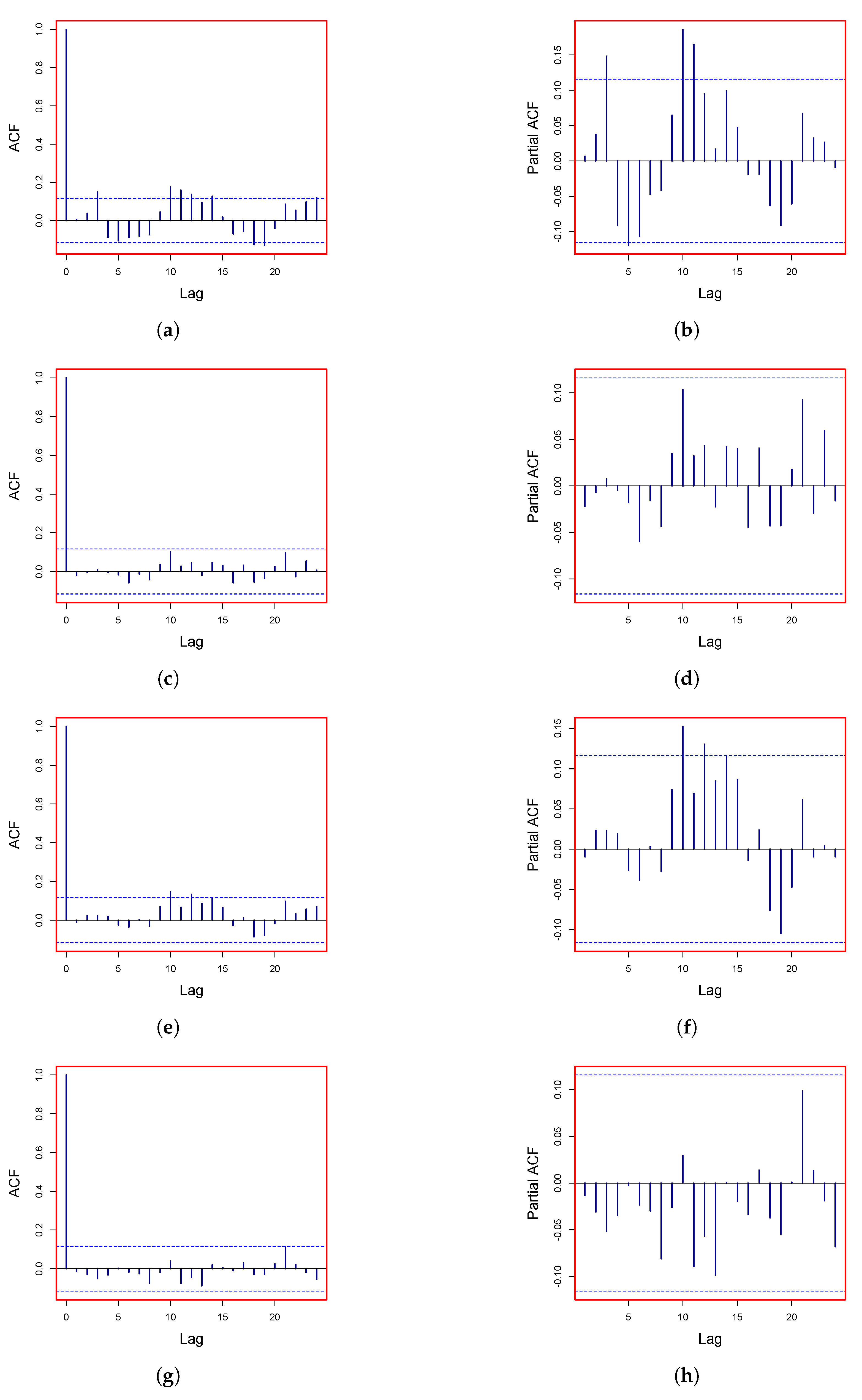
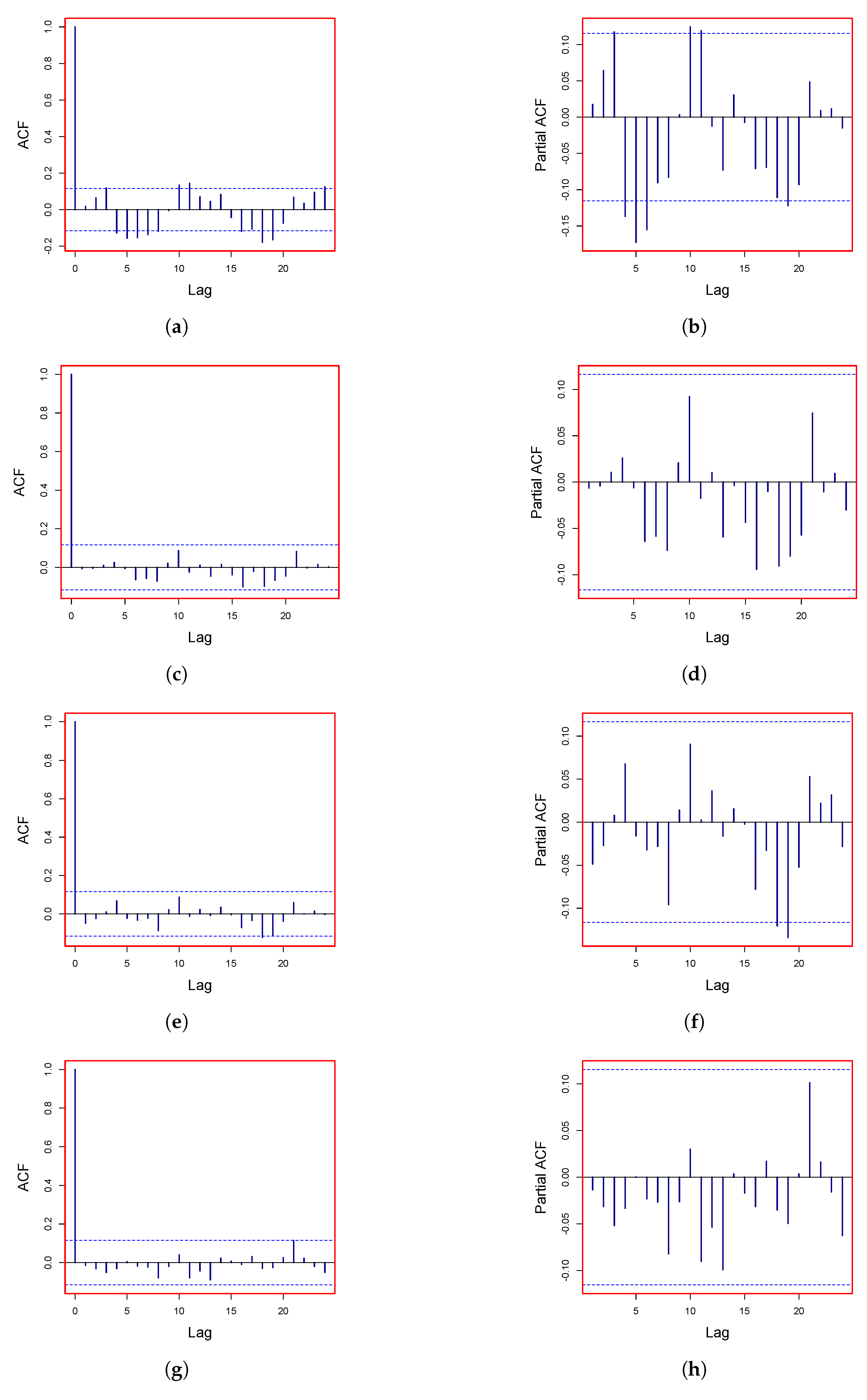
The ACF and PACF plots for the final error ${ϵ}_m$ are plotted in Figure 6 and Figure 7. In these figures, we observe that there is no longer a meaningful autocorrelation structure present in the series. Overall residuals from all models have been whitened and can be considered as satisfactory.

To verify the superiority of the results listed in Table 2, we performed Diebold and Mariano (DM) test for each pair of models [70]. The results (p-values) of DM test are listed in

Table 4. P-values for the Diabold and Marion test for same forecasts accuracy against the alternative hypothesis that model in the column is more accurate than model in the row (using squared loss function).

MODELS	P-AR	P-NPAR	P-STAR	P-ARMA	NP-AR	NP-NPAR	NP-STAR	NP-ARMA
P-AR	-	0.41	0.02	0.00	0.25	0.01	0.09	<0.01
P-NPAR	0.59	-	0.06	0.01	0.39	0.03	0.23	0.01
P-STAR	0.98	0.94	-	0.02	0.82	0.16	0.66	0.03
P-ARMA	0.99	0.99	0.98	-	0.97	0.76	0.97	0.30
NP-AR	0.75	0.61	0.18	0.03	-	0.03	0.13	0.03
NP-NPAR	0.99	0.97	0.84	0.24	0.98	-	0.92	0.21
NP-STAR	0.91	0.77	0.34	0.03	0.87	0.08	-	0.04
NP-ARMA	>0.99	0.99	0.97	0.70	0.97	0.79	0.96	-

. Each entry of the table is the p-value of a hypothesis system where the null hypothesis assumes no difference in the accuracy of the predictor in the column/row against the alternative hypothesis that the predictor in the column is more accurate than predictor in the row. In this table, we can see that, among all possible combination models, P-ARMA and NP-ARMA models at 5% level of significance are statically better than the rest, except when comparing them to NP-NPAR.

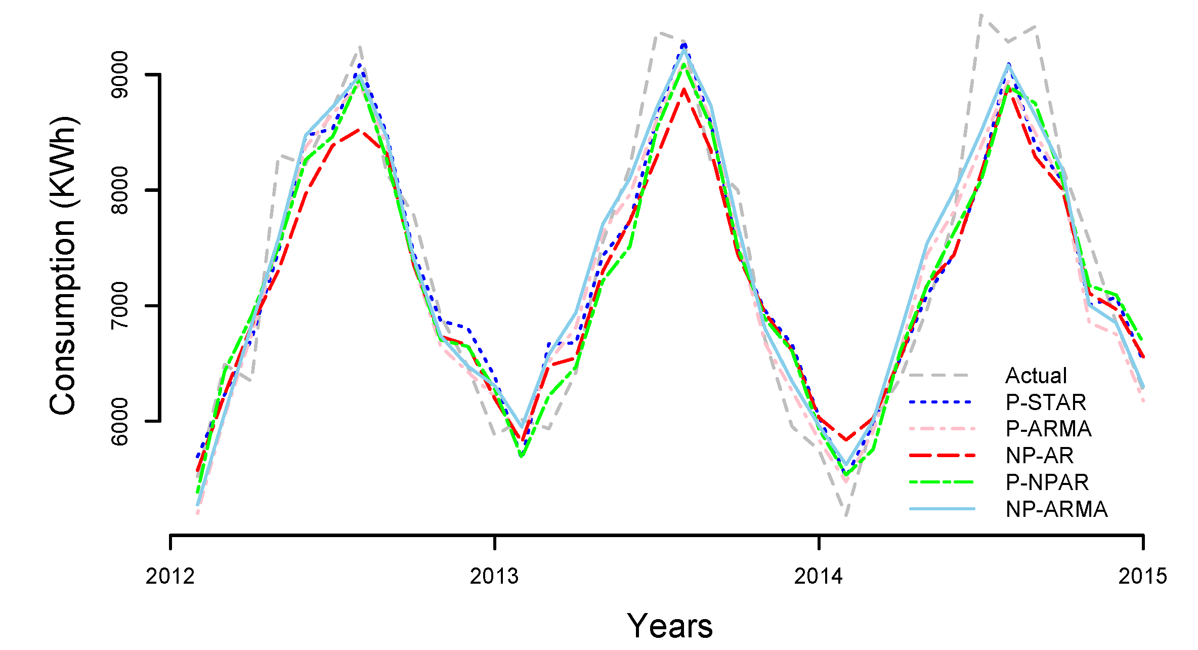
Forecasted values from four best combination models are plotted in Figure 8. In this plot, we can see that the forecasted values follow the observed values of electricity consumption very well. Finally, it is worth mentioning that our best MAPE values are comparatively batter than those cited in other works. For example, using four different models for Pakistan electricity consumption forecasting, Yasmeen and Sharif [32] reported a minimum MAPE value of 5.99, a value 24% greater than our minimum MAPE value of 4.83. For the total consumption forecast of Pakistan, Hussain et al. [71] reported a RMSE value of 1796.9 that is considerably higher than our value of 460.80.

5. Conclusions

The main aim of this study was to forecast one month ahead electricity consumption for Pakistan using component estimation technique. To this end, the electricity consumption time series was divided into two major components, i.e., deterministic and stochastic. The deterministic component consists of trend (long-run) and yearly periodicity and was modeled by both parametric and nonparametric approaches. For the stochastic component, we used four univariate time series models, including AutoRegressive (AR), Nonparametric AutoRegressive (NPAR), Smooth Transition AutoRegressive (STAR), and AutoRegressive Moving Average (ARMA) models. The estimation of both deterministic and stochastic components led us to compare eight different combinations of these models. To check the forecasting performance of all models, consumption data from Pakistan were used, and one month ahead post-sample forecasts were obtained for four years. The predicting accuracy of the models was evaluated through MAE, MAPE, and RMSE. To evaluate the significance of the differences in the forecasting performance of the models, the Diebold and Mariano test was performed. The results show that the component based estimation approach is highly effective for modeling and forecasting electricity consumption. Among all possible models, P-ARMA and NP-ARMA produced the best results, while NP-NPAR model remained competitive to the best. Finally, our forecasting results are comparatively batter than those cited in other works. In the future, this study can be extended by exploring the effects on out-of-sample forecasting when other exogenous variables are included in the models.

References

- Hahn, H.; Meyer-Nieberg, S.; Pickl, S. Electric load forecasting methods: Tools for decision making. Eur. J. Oper. Res. 2009, 199, 902–907. [Google Scholar] [CrossRef]
- Solomon, S. Climate Change 2007—The Physical Science Basis: Working Group I Contribution to the Fourth Assessment Report of the IPCC; Cambridge University Press: Cambridge, UK, 2007; Volume 4. [Google Scholar]
- Bianco, V.; Manca, O.; Nardini, S. Electricity consumption forecasting in Italy using linear regression models. Energy 2009, 34, 1413–1421. [Google Scholar] [CrossRef]
- Mohamed, Z.; Bodger, P. Forecasting electricity consumption in New Zealand using economic and demographic variables. Energy 2005, 30, 1833–1843. [Google Scholar] [CrossRef] [Green Version]
- Srinivasan, D.; Tan, S.S.; Cheng, C.; Chan, E.K. Parallel neural network-fuzzy expert system strategy for short-term load forecasting: System implementation and performance evaluation. IEEE Trans. Power Syst. 1999, 14, 1100–1106. [Google Scholar] [CrossRef]
- Kyriakides, E.; Polycarpou, M. Short Term Electric Load Forecasting: A Tutorial. In Trends in Neural Computation; Springer: Berlin/Heidelberg, Germany, 2007; pp. 391–418. [Google Scholar]
- Gonzalez-Romera, E.; Jaramillo-Moran, M.A.; Carmona-Fernandez, D. Monthly electric energy demand forecasting based on trend extraction. IEEE Trans. Power Syst. 2006, 21, 1946–1953. [Google Scholar] [CrossRef]
- Ringwood, J.V.; Bofelli, D.; Murray, F.J. Forecasting electricity demand on short, medium and long time scales using neural networks. Intel Robot Syst. 2001, 21, 315–322. [Google Scholar]
- Jia, N.; Yokoyama, R.; Zhou, Y.; Gao, Z. A flexible long-term load forecasting approach based on new dynamic simulation theory—GSIM. Int. J. Electr. Power Energy Syst. 2001, 23, 549–556. [Google Scholar] [CrossRef]
- McSharry, P.E.; Bouwman, S.; Bloemhof, G. Probabilistic forecasts of the magnitude and timing of peak electricity demand. IEEE Trans. Power Syst. 2005, 20, 1166–1172. [Google Scholar] [CrossRef]
- Papalexopoulos, A.D.; Hesterberg, T.C. A regression-based approach to short-term system load forecasting. IEEE Trans. Power Syst. 1990, 5, 1535–1547. [Google Scholar] [CrossRef]
- Abdel-Aal, R. Univariate modeling and forecasting of monthly energy demand time series using abductive and neural networks. Comput. Ind. Eng. 2008, 54, 903–917. [Google Scholar] [CrossRef]
- Alamaniotis, M.; Bargiotas, D.; Tsoukalas, L.H. Towards smart energy systems: Application of kernel machine regression for medium term electricity load forecasting. SpringerPlus 2016, 5, 58. [Google Scholar] [CrossRef] [PubMed] [Green Version]
- González-Romera, E.; Jaramillo-Morán, M.Á.; Carmona-Fernández, D. Forecasting of the electric energy demand trend and monthly fluctuation with neural networks. Comput. Ind. Eng. 2007, 52, 336–343. [Google Scholar] [CrossRef]
- Ucenic, C.; George, A. A Neuro-fuzzy Approach to Forecast the Electricity Demand. In Proceedings of the 2006 IASME/WSEAS International Conference on Energy & Environmental Systems, Chalkida, Greece, 8–10 May 2006; pp. 299–304. [Google Scholar]
- Chang, P.C.; Fan, C.Y.; Lin, J.J. Monthly electricity demand forecasting based on a weighted evolving fuzzy neural network approach. Int. J. Electr. Power Energy Syst. 2011, 33, 17–27. [Google Scholar] [CrossRef]
- Akay, D.; Atak, M. Grey prediction with rolling mechanism for electricity demand forecasting of Turkey. Energy 2007, 32, 1670–1675. [Google Scholar] [CrossRef]
- Wang, Q.; Wang, X.; Xia, F. Integration of Grey Model and Multiple Regression Model to Predict Energy Consumption. In Proceedings of the 2009 International Conference on Energy and Environment Technology, Guilin, China, 16–18 October 2009; Volume 1, pp. 194–197. [Google Scholar]
- Yanjun, L.; Yuliang, Z. Energy Demand Forecast of Henan Province by Using Gray Models GM (1, 1). Henan Sci. 2009, 12, 010. [Google Scholar]
- Wang, Y.; Wang, J.; Zhao, G.; Dong, Y. Application of residual modification approach in seasonal ARIMA for electricity demand forecasting: A case study of China. Energy Policy 2012, 48, 284–294. [Google Scholar] [CrossRef]
- Nawaz, S.; Iqbal, N.; Anwar, S. Modelling electricity demand using the STAR (Smooth Transition Auto-Regressive) model in Pakistan. Energy 2014, 78, 535–542. [Google Scholar] [CrossRef]
- Ohtsuka, Y.; Oga, T.; Kakamu, K. Forecasting electricity demand in Japan: A Bayesian spatial autoregressive ARMA approach. Comput. Stat. Data Anal. 2010, 54, 2721–2735. [Google Scholar] [CrossRef]
- Al-Qahtani, F.H.; Crone, S.F. Multivariate k-nearest NeighbourRegression forTime Series Data—A Novel Algorithm for Forecasting UK Electricity Demand. In Proceedings of the 2013 International Joint Conference on Neural Networks (IJCNN), Dallas, TX, USA, 4–9 August 2013; pp. 1–8. [Google Scholar]
- Vu, D.H.; Muttaqi, K.M.; Agalgaonkar, A. A variance inflation factor and backward elimination based robust regression model for forecasting monthly electricity demand using climatic variables. Appl. Energy 2015, 140, 385–394. [Google Scholar] [CrossRef] [Green Version]
- Wang, J.; Zhu, W.; Zhang, W.; Sun, D. A trend fixed on firstly and seasonal adjustment model combined with the ε-SVR for short-term forecasting of electricity demand. Energy Policy 2009, 37, 4901–4909. [Google Scholar] [CrossRef]
- Hong, W.C.; Dong, Y.; Lai, C.Y.; Chen, L.Y.; Wei, S.Y. SVR with hybrid chaotic immune algorithm for seasonal load demand forecasting. Energies 2011, 4, 960–977. [Google Scholar] [CrossRef] [Green Version]
- Wang, Y.W. An artificial chromosomes embedded genetic algorithms for smart grid power demand forecast. J. Ind. Intell. Inf. 2015, 3. [Google Scholar] [CrossRef]
- Wang, L.; Zeng, Y.; Chen, T. Back propagation neural network with adaptive differential evolution algorithm for time series forecasting. Expert Syst. Appl. 2015, 42, 855–863. [Google Scholar] [CrossRef]
- Qiu, X.; Ren, Y.; Suganthan, P.N.; Amaratunga, G.A. Empirical mode decomposition based ensemble deep learning for load demand time series forecasting. Appl. Soft Comput. 2017, 54, 246–255. [Google Scholar] [CrossRef]
- Chen, J.F.; Lo, S.K.; Do, Q.H. Forecasting monthly electricity demands: An application of neural networks trained by heuristic algorithms. Information 2017, 8, 31. [Google Scholar] [CrossRef] [Green Version]
- Shah, I.; Lisi, F. Forecasting of electricity price through a functional prediction of sale and purchase curves. J. Forecast. 2020, 39, 242–259. [Google Scholar] [CrossRef]
- Yasmeen, F.; Sharif, M. Forecasting electricity consumption for Pakistan. Int. J. of Emerg. Technol. Adv. Eng. 2014, 4, 496–503. [Google Scholar]
- Al-Saba, T.; El-Amin, I. Artificial neural networks as applied to long-term demand forecasting. Artif. Intell. Eng. 1999, 13, 189–197. [Google Scholar] [CrossRef]
- Abdel-Aal, R.; Al-Garni, A. Forecasting monthly electric energy consumption in eastern Saudi Arabia using univariate time-series analysis. Energy 1997, 22, 1059–1069. [Google Scholar] [CrossRef]
- Ali, M.; Iqbal, M.J.; Sharif, M. Relationship between extreme temperature and electricity demand in Pakistan. Int. J. Energy Environ. Eng. 2013, 4, 36. [Google Scholar] [CrossRef] [Green Version]
- Mostafapour, E.; Panahi, M.; Farsadi, M. A Hybrid “k-means, VSS LMS” Learning Method for RBF Network in Short-term Load Forecasting. In Proceedings of the 2015 9th International Conference on Electrical and Electronics Engineering (ELECO), Bursa, Turkey, 26–28 November 2015; pp. 961–965. [Google Scholar]
- Elattar, E.E.; Goulermas, J.; Wu, Q.H. Electric load forecasting based on locally weighted support vector regression. IEEE Trans. Syst. Man Cybernet. Part C (Appl. Rev.) 2010, 40, 438–447. [Google Scholar] [CrossRef]
- Ghiassi, M.; Zimbra, D.K.; Saidane, H. Medium term system load forecasting with a dynamic artificial neural network model. Electr. Power Syst. Res. 2006, 76, 302–316. [Google Scholar] [CrossRef]
- Sobhani, M.; Campbell, A.; Sangamwar, S.; Li, C.; Hong, T. Combining weather stations for electric load forecasting. Energies 2019, 12, 1510. [Google Scholar] [CrossRef] [Green Version]
- Lisi, F.; Shah, I. Forecasting next-day electricity demand and prices based on functional models. Energy Syst. 2019, 1–30, In Press. [Google Scholar] [CrossRef]
- Kulakov, S. X-model: Further development and possible modifications. Forecasting 2020, 2, 2. [Google Scholar] [CrossRef] [Green Version]
- Shah, I.; Lisi, F. Day-ahead Electricity Demand Forecasting with Non-parametric Functional Models. In Proceedings of the 2015 12th International Conference on the European Energy Market (EEM), Lisbon, Portugal, 19–22 May 2015; pp. 1–5. [Google Scholar]
- Shah, I.; Iftikhar, H.; Ali, S.; Wang, D. Short-Term Electricity Demand Forecasting Using ComponentsEstimation Technique. Energies 2019, 12, 2532. [Google Scholar] [CrossRef] [Green Version]
- Jamil, F. On the electricity shortage, price and electricity theft nexus. Energy Policy 2013, 54, 267–272. [Google Scholar] [CrossRef]
- Malik, A. Power Crisis in Pakistan: A Crisis in Governance? Technical report; Pakistan Institute of Development Economics: Islamabad, Pakistan, 2012. [Google Scholar]
- Ullah, A.; Khan, K.; Akhtar, M. Energy intensity: A decomposition exercise for Pakistan. Pak. Dev. Rev. 2014, 53, 531–549. [Google Scholar]
- National Electric Power Regulatory Authority. (2011a); Report. 2011, Volume 46, pp. 1583–1599. Available online: https://nepra.org.pk/tariff/Tariff/KESC/2012/TRF-133%20KESC20Dec-2011%2028-05-2012%204778-82.PDF (accessed on 30 April 2020).
- Kessides, I.N. Chaos in power: Pakistan’s electricity crisis. Energy Policy 2013, 55, 271–285. [Google Scholar] [CrossRef]
- National Power Policy of Pakistan; Report. 2013, pp. 1–26. Available online: https://policy.asiapacificenergy.org/sites/default/files/National%20Power%20Policy%202013.pdf (accessed on 30 April 2020).
- An Overview of Electricity Sector In Pakistan; Islamabad Chamber of Commerce and Industry: Islamabad, Pakistan, 2015; Technical Report.
- Pakistan Economic Survey 2015–16; Report. 2016; pp. 1–10. Available online: http://www.finance.gov.pk/survey/chapters_16/highlights_2015_16.pdf (accessed on 30 April 2020).
- Weron, R.; Bierbrauer, M.; Trück, S. Modeling electricity prices: Jump diffusion and regime switching. Phys. A Stat. Mech. Its Appl. 2004, 336, 39–48. [Google Scholar] [CrossRef] [Green Version]
- De Jong, C. The nature of power spikes: A regime-switch approach. Stud. Nonlinear Dyn. Econ. 2006, 10. [Google Scholar] [CrossRef]
- Kosater, P.; Mosler, K. Can Markov regime-switching models improve power-price forecasts? Evidence from German daily power prices. Appl. Energy 2006, 83, 943–958. [Google Scholar] [CrossRef] [Green Version]
- Nagbe, K.; Cugliari, J.; Jacques, J. Short-term electricity demand forecasting using a functional state space model. Energies 2018, 11, 1120. [Google Scholar] [CrossRef] [Green Version]
- Dordonnat, V.; Koopman, S.J.; Ooms, M. Intra-daily smoothing splines for time-varying regression models of hourly electricity load. J. Energy Mark. 2010, 3, 17. [Google Scholar] [CrossRef]
- Shah, I. Modeling and Forecasting Electricity Market Variables. Ph.D. Thesis, University of Padova, Padova, Italy, 2016. [Google Scholar]
- Pilipovic, D. Energy Risk: Valuing and Managing Energy Derivatives; McGraw-Hill: New York, NY, USA, 1998; Volume 300. [Google Scholar]
- Escribano, A.; Ignacio Pe na, J.; Villaplana, P. Modelling electricity prices: International evidence. Oxf. Bull. Econ. Stat. 2011, 73, 622–650. [Google Scholar] [CrossRef] [Green Version]
- Veraart, A.E.; Veraart, L.A. Modelling Electricity Day-ahead Prices by Multivariate Lévy Semistationary Processes. In Quantitative Energy Finance; Springer: New York, USA, 2014; pp. 157–188. [Google Scholar]
- Lucia, J.J.; Schwartz, E.S. Electricity prices and power derivatives: Evidence from the nordic power exchange. Rev. Derivat. Res. 2002, 5, 5–50. [Google Scholar] [CrossRef]
- Liu, J.M.; Chen, R.; Liu, L.M.; Harris, J.L. A semi-parametric time series approach in modeling hourly electricity loads. J. Forecast. 2006, 25, 537–559. [Google Scholar] [CrossRef]
- Dickey, D.A.; Fuller, W.A. Distribution of the estimators for autoregressive time series with a unit root. J. Am. Stat. Assoc. 1979, 74, 427–431. [Google Scholar]
- Phillips, P.C.; Perron, P. Testing for a unit root in time series regression. Biometrika 1988, 75, 335–346. [Google Scholar] [CrossRef]
- Shahbaz, M.; Lean, H.H. The dynamics of electricity consumption and economic growth: A revisit study of their causality in Pakistan. Energy 2012, 39, 146–153. [Google Scholar] [CrossRef] [Green Version]
- Cavaliere, G. Unit root tests under time-varying variances. Econ. Rev. 2005, 23, 259–292. [Google Scholar] [CrossRef]
- Bosco, B.; Parisio, L.; Pelagatti, M.; Baldi, F. Long-run relations in European electricity prices. J. Appl. Econ. 2010, 25, 805–832. [Google Scholar] [CrossRef]
- Wasserman, L.A. All of Nonparametric Statistics; Springer: New York, USA, 2006. [Google Scholar]
- Teräsvirta, T. Specification, estimation, and evaluation of smooth transition autoregressive models. J. Am. Stat. Assoc. 1994, 89, 208–218. [Google Scholar]
- Diebold, F.; Mariano, R. Comparing predictive accuracy. J. Bus. Econ. Stat. 1995, 13, 253–263. [Google Scholar]
- Hussain, A.; Rahman, M.; Memon, J.A. Forecasting electricity consumption in Pakistan: The way forward. Energy Policy 2016, 90, 73–80. [Google Scholar] [CrossRef]
Figure 1.
Pakistan electricity consumption (kWh): (a) Electricity consumption time series for the period January 1990 to December 2016; (b) yearly periodicity for the period January 2000 to December 2003; (c) box plot for monthly observation for the period January 1990 to December 2015; and (d) seasonal plot for the period January 1990 to December 2015.
Figure 2.
Pakistan electricity consumption series with superimposed fitted deterministic component (Dm) for parametric (a) and nonparametric (b) methods, and stochastic component (Sm) from parametric case (c) and from nonparametric case (d).
Figure 3.
Components estimation: Trend (long-run) component estimated parametrically (a) and nonparametrically (b) and yearly periodicity component estimated nonparametrically (c) and parametrically (d).
Figure 4.
MAPE values of one month ahead post-sample forecasts for all models.
Figure 5.
One month ahead post-sample forecasts MAPEs with respect to seasons of the year.
Figure 6.
ACF and PACF for the final ∈t for P-AR (a,b), P-NPAR (c,d), P-STAR (e,f) and P-ARMA (g,h).
Figure 7.
ACF and PACF for the final ∈t for NP-AR (a,b), NP-NPAR (c,d), NP-STAR (e,f) and NP-ARMA (g,h).
Figure 8.
Actual and forecasted electricity consumption for only five best models (P-STAR. P-ARMA, NP-AR, P-NPAR, and NP-ARMA) for the period January 2011–December 2014 (right).