Forecasting Social Conflicts in Africa Using an Epidemic Type Aftershock Sequence Model

Abstract

We propose to view social conflicts in Africa as having similarities with earthquake occurrences and hence to consider the spatial-temporal Epidemic Type Aftershock Sequence (ETAS) model. The parameters of this highly parameterized model are estimated through simulated annealing. We consider data for 2012 to 2016 to calibrate the model for four African regions separately, and we consider the data for 2017 to evaluate the forecasts. These forecasts concern the amount of future large events as well as their locations. Examples of our findings are that the model predicts a cluster of large events in the Central Africa region, which was not expected based on past events, and that in particular for East Africa it apparently holds that small conflicts can trigger a larger number of conflicts.

1. Introduction and Motivation

The analysis and prediction of social conflicts is an active and important area of research. Yet, the current state of affairs is that it is not easy to find a forecasting methodology that can deliver accurate predictions, see for example [1,2,3,4].

Recently, various studies incorporating machine learning techniques, like for example [5,6,7], have indicated that certain machine learning methods can deliver accurate forecasts for social conflicts.

In this paper, we wish to add a novel forecasting tool, which is based on a self-exciting process, a tool that is also often use to predict earthquakes. Indeed, in some dimensions, social conflicts data and earthquakes data show similarities.

First, they seem to correspond to self-exciting processes. Long periods of non-activity correspond with building up tension, and once an event happens, the tension is released, perhaps causing more events. Such a triggering increases with the size of the event and may decrease over time and distance. A second similarity concerns clustering. That is, earthquakes often take place at the edge of tectonic plates and for conflicts it often occurs that conflicts are witnessed around country or region borders. Triggered events seem to occur more frequently near their previous events than further away.

To exploit these similarities, we propose to analyze social conflicts data using a popular model in the earthquake literature, and this is the so-called Epidemic Type Aftershock Sequence (ETAS) model. To illustrate, we use social conflicts data in Africa. ETAS models are a special type of a self-exciting point processes and are widely used in studying earthquake occurrences. In this model, events can occur spontaneously, and events can be triggered by other events. Each event can trigger new events, which in turn can trigger new events. The model describes the intensity and locations of spontaneous background events and the triggering dynamics.

The outline of our paper is as follows. In Section 2 we describe our sample with social conflicts data for Africa, and we suggest that indeed such data bear similarities with earthquake data. In Section 3 we discuss the model and a method to estimate its parameters. Next, we discuss ways to evaluate the quality of the model, and a method to create forecasts. Section 4 brings the ETAS model to the data for Africa where we take the data for 2012 to 2016 as the in-sample data, and we consider the data for 2017 as our forecast sample. We see that the model fits the data well, and also that out-of-sample forecasts can be informative and accurate. Section 5 concludes with limitations, as there are several, and with various avenues for further research, of which we think there are many too.

2. Social Conflicts in Africa

We obtain the conflict data from the Armed Conflict Location and Event Data (ACLED) Project (https://www.acleddata.com/data/). The project collects the dates, actors, types of violence, locations, and fatalities of all reported political violence and protest events across Africa ever since 1997. Before we can analyze the data, we need to compile a proper database. We define a social conflict (in this database) as an event which consists of four numbers, that is, the event date, location (latitude and longitude) and the number of fatalities. As exact time stamps are unavailable, we assume that each conflict happened at 12:00 noon. The complete description of methodological accuracies and definitions can be found on the ACLED website: https://www.acleddata.com/resources/methodology/.

The numbers of fatalities are estimated as the numbers reported by any source material and are not verified by the ACLED project itself. In order to be most reliable, the ACLED project uses the most conservative estimates. For example, if a news article mentions several, many or few fatalities, it is recorded as 10. Dozens is recorded as 12. If a report mentions hundreds of casualties or a massacre, it is recorded as 100. The location of a conflict is recorded as the location of the nearest town or city and if a larger region is described, the provincial capital of that region is used. Furthermore, if a conflict lasts several days, the event is recorded as a new event each day with the average number of fatalities over those days. We take the data as they are and assume that the dates, locations and numbers of fatalities are accurate.

We analyze conflicts between 2012 and 2017 with at least two fatalities. This time window and fatality range results in 17,334 events in total with around 2500 to 7000 events in each of the major African regions. This number of events should be large enough to accurately estimate the model in each region. Our estimation routine will be implemented in the SEDA software package, and this number of observations is regarded as properly sized, see [8]. Note that it is not the number of years that counts, but the number of events. Using more years of data or including events with one fatality would make model estimation computationally infeasible.

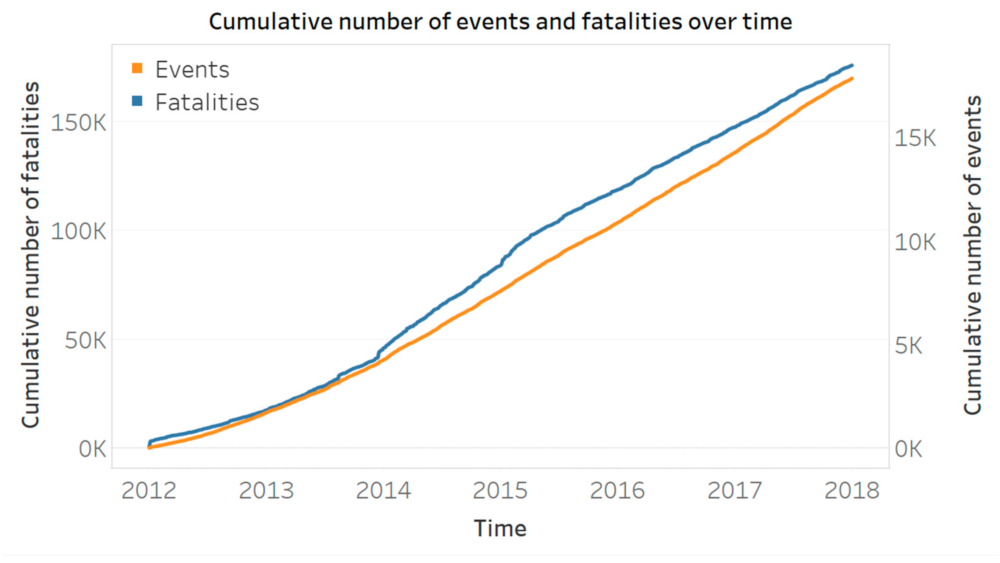
In Figure 1 we present the cumulative number of events and fatalities over time, using dual axes. We see that the average number of events per day increases slightly after 2014 but remains relatively constant over the period. The number of fatalities per event also remains relatively constant, except for an increase between 2014 and 2015, which could be addressed to the start of the Second Libyan Civil War in 2014.

To explore the spatial distribution of conflicts, we display all events in this period in a map of Africa, see Figure 2. The size of the dots represents the number of fatalities. Events with more than one hundred fatalities are in red. Figure 2 shows that there are several large clusters of events. For example, we see many events with more than a hundred fatalities in the top right corner of Nigeria, which is the area where Boko Haram is active. In the top right corner of Egypt, conflicts resulting from the Arab Spring can be seen. Furthermore, there are large clusters of conflicts around the border of Sudan with South-Sudan which associates with the South Sudanese Civil War. Other notable clusters can be found in the eastern part of the Democratic Republic of the Congo and in the south of Somalia. Overall, and as expected, we see that conflicts tend to be located more around country borders than elsewhere.

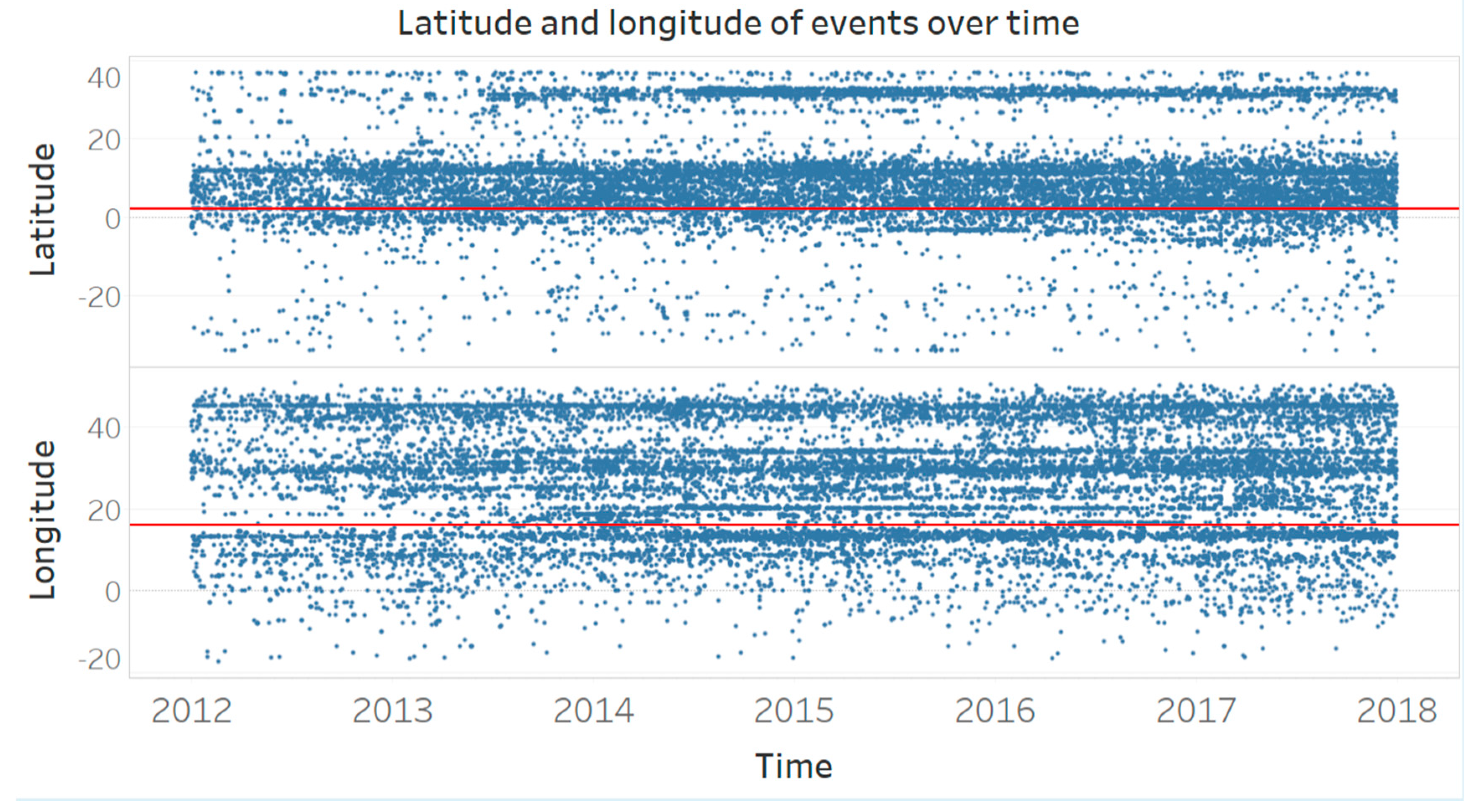
To explore the spatial distribution of the events over time, the latitude and longitude of each event are presented in Figure 3. The red lines represent the latitude and longitude of the geographical center of Africa. We see that there are more events in the northern half of Africa than in the southern half, and more events in the eastern half than in the western half. In the top panel of the graph, we see that most conflicts are clustered around the equator and that there are relatively fewer events in the south of Africa. In the bottom panel of the graph, we see that events are more evenly distributed across the longitude. Over time, however, events tend to occur around the same latitudes and longitudes. Note the appearance of events around 30 degrees latitude from 2013 onwards, which can be associated with the many conflicts resulting from the Arab Spring.

Next, we discuss the distribution of the sizes, or magnitudes, of the conflict events. In

Table 1. Fatality quantiles of events in the Armed Conflict Location and Event Data (ACLED) dataset between 2012 and 2017 with at least 2 fatalities.

Quantile	Fatalities	Quantile	Fatalities
0	2	0.91	20
1	2	0.92	22
2	2	0.93	25
3	3	0.94	28
4	3	0.95	31
5	4	0.96	38
6	6	0.97	47
7	8	0.98	58
8	10	0.99	96
9	19	1	600

, the fatality quantiles are given. It can be seen that the distribution of fatalities is skewed, that is, most events have a small number of fatalities and relatively few events have a large number of fatalities. Over half of the events have 4 fatalities or less, 99% of the events has up to 100 fatalities and the largest event has 600 fatalities.

The ETAS model we will consider for our data originates from [9,10] and it assumes that the magnitudes of events follow the Gutenberg–Richter law. So, before we can apply our model, we align the data. This law is given by:

$$N={10}^{a-bM}$$

(1)

where N is the number of events with magnitude M or larger and a and b are constants. If one were to estimate these parameters for actual data, the value of b is typically close to 1 and in that case, events with one larger magnitude are ten times less likely to happen. To make the conflicts follow this law, we group the events based on their fatalities and assign magnitudes to each group in such a way that the number of events at each increasing magnitude decreases by a factor of ten. The derivation of the correspondence between fatalities and magnitudes is given in the Appendix A.

In the end, we obtain the magnitude distribution for the conflict events as given in the

Table 2. The magnitude distribution of the social conflict data. For each magnitude there is the corresponding number of fatalities, the percentage of events expected by the Gutenberg–Richter law, the observed percentage of events, the expected absolute number of events and the observed absolute number of events. The full table appears in the Appendix A.

Magnitude	Fatalities	% Expected	% Observed	Expected	Observed
3	2	20.57	26.94	3565	4669
4	22	2.06	1.77	357	306
5	100	0.21	0.33	36	57
6	400	0.02	0.00	4	0
7	600	0.00	0.01	0	1

, where we adopt a where the magnitude range is 3.0, 3.1, 3.2, …, 7. The full table is given in the Appendix A. This table only shows the integer magnitudes. In the left two columns, the correspondence between fatalities and magnitude is shown. The next two columns show the percentage of events expected by the Gutenberg–Richter law at each magnitude, together with the observed percentage. The last two columns show the expected and observed absolute numbers of events. We see that with each magnitude step, the percentage and number of events decreases roughly by a factor ten. It should be noted that we follow the tradition in the earthquake literature, also because we have no other benchmark.

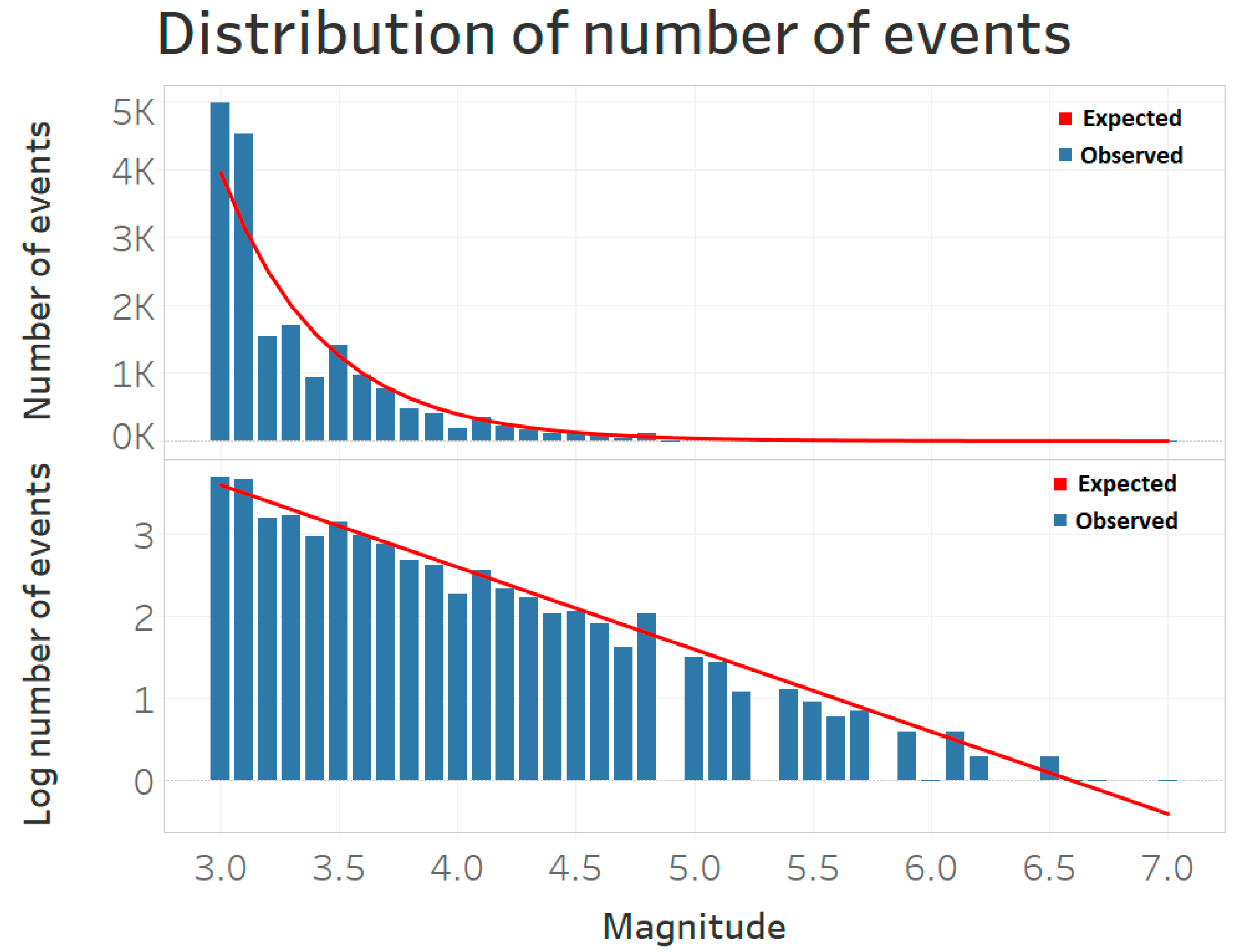
The expected and observed number of events for each magnitude is presented in Figure 4, together with the log 10 of these numbers (bottom panel). If the magnitude distribution follows the Gutenberg–Richter law, the blue bars in the figure should correspond with the red line. Estimating the b value in (1) using Maximum Likelihood results in a value of 0.95 with standard error 0.01. Hence, this way of assigning magnitudes to fatalities gives a magnitude distribution that resembles the distribution of an earthquake catalog (which is the way that data are called in the earthquake literature), which is assumed by the model.

3. The ETAS Model

In this section we will discuss the ETAS model used to study the social conflicts. The model parameters will be estimated using the simulated annealing algorithm proposed in [10]. Furthermore, we will discuss several ways of testing the model and describe the way to make forecasts.

3.1. Representation

Earthquake occurrences have been modeled using a variety of point process models and the most popular is the Epidemic Type Aftershock Sequence (ETAS) model. In this model, events are divided into two categories. There are background events and triggered events. Background events are events that occur spontaneously. Triggered events occur as a result of other events. Each event can trigger new events, which in turn can again trigger new events. [11] provide a list of common features of ETAS models, and these are: (a) the occurrence rate of background events depends on location and magnitude, but is independent of time; (b) the magnitude of a background event is independent of its location; (c) each event produces offspring events independently and the number of offspring events produced depends on the magnitude of the event; (d) the occurrence time of an offspring event depends only on the time difference from its ancestor and is independent of the magnitude; (e) the location of an offspring event depends on the location of its ancestor; and (f) the magnitude of an offspring event is independent of the magnitude of its ancestor. These six features explain the design of the ETAS model.

One of the first models is the temporal ETAS model proposed by [9] to describe the origin times and magnitudes of earthquakes. This model has been extended to also include the spatial aspect of earthquake occurrences in [10] and [11]. Below, we will use this spatial-temporal ETAS model for the social conflicts.

The occurrences of events can often be completely described by the conditional intensity function of the process, which gives the probability of an event with a certain magnitude occurring at a specific place at a specific time. This function often consists of two parts, that is, a part describing the occurrence rate of background events and another part describing the way events trigger new events.

In our study we use the model as defined in [8], which is similar to the one in [10]. The conditional intensity function in this model is given by:

$$\lambda \left(t,\mu ,x,y|H_t\right)=\left(\mu ·u\left(x,y\right)+{\displaystyle \sum }_{T_i<t}g\left(t,x,y;T_i,M_i,X_i,Y_i\right)\right)f\left(m\right)$$

(2)

where event i is described by a time $T_i$, location $\left(X_i,Y_i\right)$ and magnitude $M_i$. This intensity function consists of three parts, that is, the spatial background distribution $u\left(x,y\right)$, the decay function $g(t,x,y;H_i$) and the magnitude probability density function $f\left(m\right)$. Each of these components will be discussed next.

The magnitude probability density function is based on the Gutenberg–Richter law (hence the reason to scale that data as in the Appendix A) and is given by:

$$f\left(m\right)=\frac{\beta ·\exp \left(-\beta \left(m-M_c\right)\right)}{1-\exp \left(-\beta \left(M_{max}-M_c\right)\right)}$$

(3)

where $\beta =b\log \left(10\right)$ and $M_{max}$is the magnitude of the largest event. The $M_c$ refers to the minimum magnitude for which the catalog is complete, that is, the magnitude for which all events with magnitude $M\ge M_c$ are recorded.

The rate at which event i can trigger new events decreases with distance and time from that event. This is described by the decay function $g(t,x,y;H_i$) which is given by:

$$g\left(t,x,y;H_i\right)=\frac{k·\exp \left(\alpha \left(M_i-M_c\right)\right)}{{(t-T_i+c)}^p}·\frac{c_{d,q,\gamma }^i}{{(r_i^2+d^2·\exp \left(2\gamma \left(M_i-M_c\right)\right))}^q}$$

(4)

Here, $H_i$ is the history of events before event i. The decay function in (4) consists of two parts. The first part describes the temporal decay rate and the second part the spatial distribution. The temporal decay is governed by the parameters {$\alpha ,c,k,p$}. The parameter $\alpha$ measures the influence of excess magnitude $M_i-M_c$ in generating offspring events and k is a normalizing constant for the number of offspring events. A small value for $\alpha$ implies that the effect of the magnitude on triggering new events is small, and thus that smaller events can trigger a larger amount of events more easily, see [12]. As usual, we assume that larger events cause more aftershocks than smaller events, that is, $\alpha >0$. As the number of offspring events cannot be negative, we have that also k > 0. It is hard to register all aftershocks after a large event and this incompleteness is measured by the parameter c. Finally, the parameter p is the rate of decay over time. We would expect p > 1, as this implies that each event can only generate a finite number of offspring events.

The second part of (4) determines the spatial probability distribution. The term $r_i$ is the distance to event i and $c_{d,q,\gamma }^i$ is a normalization constant such that the integral over the entire region equals 1. The term $d^2·\exp \left(2\gamma \left(M_i-M_c\right)\right)$ measures the influence of magnitude on the spatial extent of the aftershock region for event i. Similar to p, the parameter q measures the spatial decay rate. If we ignore any spatial components in the model and integrate over the entire region, the right-hand term of (4) becomes 1 and we obtain the decay function for the temporal model in [9].

The first term in (2) consists of a parameter $\mu$and the spatial background distribution u(x, y). The parameter $\mu$ is the Poisson rate of background events. The background distribution determines how these events are distributed across the region. We will estimate the spatial background distribution following the procedure in [8], which is largely based on the iterative kernel method proposed by [13]. For this, the region of interest is first divided into $N_c$ cells $C_i \left(i=1,2,\dots ,N_c\right)$ to make a discrete approximation. The cells are of size 0.5 × 0.5 degrees latitude/longitude, which corresponds to an area of approximately 55 × 55 = 3025 square kilometers. The background rate can vary among cells but is assumed to be homogeneous within each cell. We can then write $u\left(x,y\right)=u_i/A_i$where $u_i$ is the probability of a background event occurring in cell i with area $A_i$.

The probabilities $u_i$ are estimated using the iterative kernel method proposed by [13], which uses the following function for the background distribution, that is,

$$\mu \left(x,y\right)=\frac{1}{T}{\displaystyle \sum }_{j=1}^N\left(1-{\rho }_j\right)\frac{1}{2\pi d_j}\exp \left(-\frac{{(x-x_j)}^2+{(y-y_j)}^2}{2d_j^2}\right)$$

(5)

where T is the length of the study period, N the total number of events, ${\rho }_j$ is the probability that event j is a triggered event and $d_j$ is a variable bandwidth. The probability ${\rho }_j$ is given by the ratio between the intensity produced by all previous events and the total intensity at that time and place, that is,

$${\rho }_j=\frac{{{\displaystyle \sum }}_{i=1}^{j-1}g(t_j-t_i,x_j-x_i,y_j-y_i|m_i)}{\lambda (t_j,x_j,y_j|H_{t_j})}$$

(6)

Finally, $d_j$ is a variable bandwidth defined as the smallest disk around event j which includes at least $n_p=10$ events, as in [11]. This way, events happening in rural areas have a further reaching effect than events that happen in densely populated areas, which makes regions with high and low event densities more comparable. Following [14], we can use (5) to estimate the probabilities $u_i$ by:

$$u_i=\frac{\mu \left(X_i,Y_i\right)}{{{\displaystyle \sum }}_{j=1}^{N_c}\mu \left(X_j,Y_j\right)}, i=1,2,\dots ,N_c$$

(7)

These probabilities then give the spatial background distribution, where the sum over all cells equals 1. Together with the average background rate $\mu$, the decay function $g\left(t,x,y;H_i\right)$ and the magnitude distribution f (m), we now have described the conditional intensity function of the process. This function will be used for calculating the maximum log likelihood which gives the parameter estimates.

The log-likelihood function is given by [11], and it reads as:

$$\log L\left(\theta |H_t\right)={\displaystyle \sum }_{i=1}^{N}ln\left[\lambda (T_i,X_i,Y_i|H_{T_i})\right]-{{\displaystyle \iiint }}_{T,R}\lambda \left(t,x,y|H_t\right)dtdxdy$$

(8)

For the calculation of the log likelihood, the background probabilities $u_i$ from (7) are needed for the cells in which an event has taken place.

Hence, the parameters of the model are $\left\{\mu ,k,p,c,\alpha ,d,q,\gamma ;u_i, i=1,2,\dots ,N_c^{’}\right\}$ where $N_c^{’}$ is the subset of nonempty cells. These parameters can be estimated by maximizing the log likelihood function using the simulated annealing algorithm, which will be discussed below.

Due to the high dimensionality of the likelihood function, there is a chance that a parameter is not identified and becomes arbitrarily large or small during the estimation. Therefore, we will impose certain parameter restrictions on the eight parameters in the model. These restrictions are based on the restrictions used for modeling earthquake occurrences and on values that are physically desirable, see [10]. These restrictions are given in

Table 3. Parameter restrictions in our Epidemic Type Aftershock Sequence (ETAS) model. These restrictions are based on the restrictions used for modeling earthquake occurrences and on values that are physically desirables, see [10].

Parameter	Lower Bound	Upper Bound
$\mu$	0	1
k	0.001	0.1
p	0.5	2
c	1.00 × 10−5	0.1
$\alpha$	0	2
d	0.01	1
q	1	3
$\gamma$	0	2

. The branching ratio of the process gives the average number of events triggered by an event and is given by [8] and equals:

$$\varphi ={{\displaystyle \int }}_0^{\infty }{{\displaystyle \int }}_{M_c}^{M_{max}}\frac{k·\exp (\alpha \left(M_i-M_c\right)}{{(t+c)}^p}f\left(m\right)dmdt$$

(9)

If $\varphi >1$ due to $p<1$, events are generated faster than they die out and the process becomes explosive. The four parameters in the temporal component, $\alpha$, p, c, and k influence the number of events in the simulated catalogs. Furthermore, the parameter $\mu$ has a positive linear effect on the number of events and the parameters that determine the spatial decay, d, $\gamma$and q have no effect on the number of events. The spatial parameters describe the distribution of the events over the region. A higher value for $\alpha$ and k lead to more events and a higher value for c leads to fewer events. For the temporal decay rate p there is a small region in which the process is not explosive. However, the size of this parameter region varies depending on the values of the other parameters.

3.2. Estimation

The parameters will be estimated using a simulated annealing algorithm, which is a method for approximating the global optimum of a given function. It originates from annealing in metallurgy, describing the physical process of reducing defects by heating and then slowly cooling the material. Even though this method is unlikely to find the optimal solution, it can often find a very good approximation of the optimum. In particular, it can be preferable over (quasi) Newton methods in situations with a large number of independent variables like in our case. As the algorithm finds a good solution in a relatively short amount of time, we can run it many times, providing a probability distribution for the parameters and the background distribution. These can be used to evaluate model uncertainties. We will run the algorithm $N_{SIM}=100$ times.

The algorithm starts by generating a random solution, after which it searches for a new point in that neighborhood. This search is based on a probability distribution that depends on the so called temperature of the process. The method accepts all points that raise the objective function (in case of maximization) and also accepts points that lower the objective, with a certain probability. As such, it avoids being trapped in local maxima. By decreasing the temperature, the probability of accepting a worse solution is lowered when the solution space is explored.

More formally, we adopt the simulated annealing procedure used to estimate the ETAS models as described in [13]. It consists of an initialization, a loop and a cooling scheme.

To initialize set the count $k=0$ and generate a random starting point ${\overrightarrow{\theta }}_{opt}$ and set the initial temperature $T_0>0$. The starting temperature must be high enough that any solution can be selected and is calculated based on the function to be optimized, see [15].

The loop is a random search for a better solution around the local maximum. First, set ${\overrightarrow{\theta }}_k={\overrightarrow{\theta }}_{opt}$ and generate the next candidate $\overrightarrow{y}$ from a multi-dimensional Cauchy distribution G. We move to this point with a certain probability. Sample $z\in \left[0,1\right]$ uniformly and move to the newly generated point if $z\le A\left({\overrightarrow{\theta }}_{opt},\overrightarrow{y}, T_k\right)$, where the acceptance function A is the Metropolis criterion in [16], that reads as:

$$A\left({\overrightarrow{\theta }}_{opt},\overrightarrow{y},T_k\right)=min\left\{1,exp\left(\frac{f\left(\overrightarrow{y}\right)-f\left({\overrightarrow{\theta }}_{opt}\right)}{T_k}\right)\right\}$$

(10)

If the log-likelihood at this new point is larger, we set this new point as the current optimum, that is,

$$LogL\left(\overrightarrow{y}|H_t\right)>LogL\left({\overrightarrow{\theta }}_{opt}|H_t\right)\to {\overrightarrow{\theta }}_{opt}=\overrightarrow{y}$$

Once a new optimum is found, the temperature is lowered according to the cooling schedule proposed in [8], that is,

$$T_k=T_{0}exp\left[-13.8·exp\left(-\frac{3.4}{D}\right)·k^{\frac{1}{D}}\right]$$

where D = 8 is the number of parameters in the model. The two constants −13.8 and 3.4 were found to provide a fast algorithm based on a simulation study in [8]. After decreasing the temperature, the loop is repeated until convergence. Events that took place before the study period can still have an effect on events inside the study period. We will therefore use a one year burn-in period when estimating the model. Hence, the estimation period consists of five years from 2012 to 2016, where 2012 will be used as a learning period and the four other years, 2013–2016, will be used as the study period. The data of the last year 2017 will be used for evaluating out-of-sample forecast performance.

3.3. Inference

If the model describes the dynamics of the conflicts well, the residuals are expected to follow a stationary Poisson process with a unit rate. The residuals are obtained by a transformation of the time axis, as in [16], that is,

$$\mathsf{\Lambda }\left(t\right)={{\displaystyle \int }}_0^t{\iint }_R{{\displaystyle \int }}_{M_c}^{M_{max}}\lambda \left(t^{\prime },x,y,m|H_{t^{\prime }}\right)d{t}^{\prime }dxdydm$$

(11)

These residuals give the expected number of events with magnitude larger than $M_c$ up to time t and in the region R. If the residuals follow a stationary Poisson process with rate one, the inter-event times follow an exponential distribution. This can be tested using a one-sided Kolmogorov–Smirnov test (KS-test). We will also perform a Wald–Wolfowitz runs test, which tests the null hypothesis that the inter-event times are stationary and not autocorrelated.

Furthermore, we can perform a visual check by plotting the number of events expected by the model against the observed number of events. This can be done for the transformed times, all events, background events and triggered events. The expected numbers of events are calculated by integrating the intensities over time, magnitude and space. The expected number of total events is given by:

$$N_{exp}^{All}\left[\theta |H_t\right]={{\displaystyle \int }}_T^{}{\iint }_R\lambda \left(t,x,y|H_t\right)dtdxdy$$

(12)

The expected number of background events is given by:

$$N_{exp}^{Back}\left[\theta |H_t\right]={{\displaystyle \int }}_T^{}{\iint }_R\mu ·u\left(x,y\right)dt=\mu \left(T_2-T_1\right)$$

(13)

and the expected number of triggered events is:

$$\begin{array}{c}{N}_{exp}^{Trig}\left[\theta |H_t\right]=N_{exp}^{All}\left[\theta |H_t\right]-N_{exp}^{Back}\left[\theta |H_t\right]\\ ={{\displaystyle \int }}_T^{}{\iint }_R\frac{k·\exp \left(\alpha \left(M_i-M_c\right)\right)}{{(t-T_i+c)}^p}·\frac{c_{d,q,\gamma }^i}{{(r_i^2+d^2·\exp \left(2\gamma \left(M_i-M_c\right)\right))}^q}dtdxdy\end{array}$$

(14)

where $T_1$ and $T_2$ are the start and end times of the sample period. Note that we also integrate over the magnitude distribution, but as the magnitudes are independent of the parameters, this integral equals one.

The observed number of all events (background + triggered) can be obtained directly. As we cannot know for certain whether an event is a background or a triggered event, we cannot count them. Therefore, the number of observed background and triggered events are calculated as the sum of the probabilities of being a background or triggered event. The probability that event i is a background event is given in [8], and it reads as:

$$Pro{b}_i^B=\frac{\mu ·u\left(X_i,Y_i\right)}{\lambda (T_i,X_i,Y_i|H_{T_i})}$$

(15)

and the probability that event i is a triggered event is given by $Pro{b}_i^T=1-Pro{b}_i^B$. The sum of these probabilities over all events determine the ‘observed’ number of background and triggered events.

The number-of-events test compares the number of events in the conflict catalog (the dataset) with the number of events expected by the model. The expected number of events and its distribution are obtained from simulating a large number of event catalogs and calculating the number of events in each of them. Specifically, this is done in the following way. Simulate $N_{SIM}=100$catalogs based on the estimated parameters in an ETAS model. Then, fit a normal distribution to the number of events in each simulated catalog. Next, calculate the median and the 95% confidence bounds, and with these we compute the probability that we observe more events than in our dataset.

Finally, we will test the performance of the model by making a forecast for the number of events and their location in the hold-out sample. We focus on events with magnitude $M_f>4$, which for the African countries data corresponds to 22 or more fatalities. For this, we simulate $N_{SIM}=100$catalogs using the empirical ETAS model and calculate the expected number of events with magnitude $M_f>4$ in each cell of the regions in the hold-out sample. The expected number of events in simulated catalog i in cell $C_j$ is given in [8], and it reads as:

$$f_{ij}={{\displaystyle \int }}_T^{}{\iint }_{C_j}{{\displaystyle \int }}_{M_f}^{M_{max}}\lambda \left(t,x,y,m|H_t^i\right)dmdxdydt$$

(16)

where $H_t^i$is the history of the process up to time t for catalog i. For each cell we then take the median number of events of all simulated catalogs as the forecast. The total number of events can then be calculated as the sum of the median number of events over all cells. The forecasted number of events and locations will then be compared with their observed number and locations to examine accuracy.

In [13], the above described estimation and evaluation methodology is examined using extensive simulations. There it is concluded that the ETAS model can be reliably implemented for simulated data. It can happen though that parameters are estimated at their boundary value, and this is not unexpected given that the ETAS model is heavily parameterized.

4. Modeling and Forecasting Social Conflicts in Africa

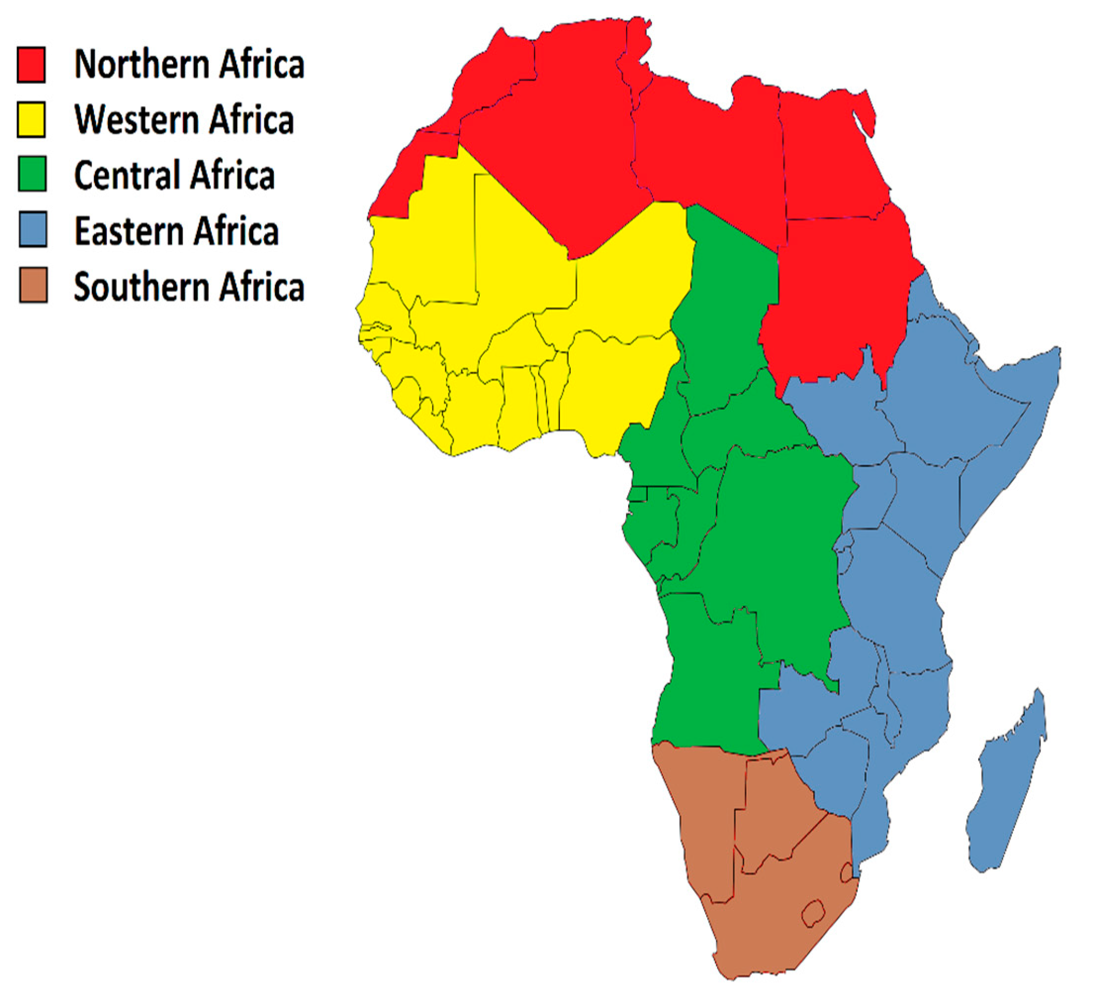
The continent of Africa is often divided in five major geographical regions. These are North-, West-, Central-, East- and South Africa. These regions are displayed in Figure 5. The numbers of events in each region for the learning period, study period, forecasting period and total, are given in

Table 4. Number of conflict events in each region for the learning period (2012), study period (2013–2016) and forecasting period (2017) and in total (2012–2017).

	North	West	Central	East	South	Total
N learning period	291	378	203	708	40	1620
N study period	3518	2164	1834	4617	117	12250
N forecasting period	612	617	589	1630	16	3464
N total	4421	3159	2626	6955	173	17334

. As the number of events in the region South Africa is too small to reasonably estimate the model, we will restrict the study to the other four major regions. Some summary statistics regarding the number of fatalities and magnitudes are given in

Table 5. Summary statistics of the magnitudes and number of fatalities in each region. The columns are the minimum (Min.), the first quantile (1st Q.), the median (Med.), Mean, third quantile (3rd Q.) and the maximum (Max.).

	Region	Min.	1st Q.	Med.	Mean	3rd Q.	Max.
Magnitude
	North	3.0	3.0	3.2	3.4	3.5	6.1
	West	3.0	3.1	3.2	3.4	3.7	7
	Central	3.0	3.1	3.2	3.3	3.5	6.1
	East	3.0	3.0	3.2	3.3	3.5	6.7
Fatalities
	North	2	2	4	10	10	411
	West	2	3	5	13	12	600
	Central	2	3	4	9	10	420
	East	2	2	4	9	10	598

. This last table shows that the size of events is quite similarly distributed in each region.

As the model assumes the magnitude probability density function based on the Gutenberg–Richter law in (1), we check whether this assumption more or less holds for the catalogs in each region. If it deviates too much, we might assume the wrong magnitude distribution for the data. For this, we estimate the parameter b in (1) for each region, and the estimation results are given in

Table 6. Maximum likelihood estimates of the parameter b in the Gutenberg–Richter law in (1).

Region	b	Standard Error
North	0.956	0.025
West	0.854	0.024
Central	0.990	0.034
East	1.006	0.022

. As the value of b is close to one for each region, we continue with the assumed probability density function in the conditional intensity function in (2). Due to an unfortunate bug in the software, events with a negative longitude cause an error. We will therefore restrict our study region to the right side of the prime meridian. This means that out of a total of 17,829 events, 495 events will be omitted in North- and West Africa. This should not affect the estimation results in a large way as this number of events is relatively small.

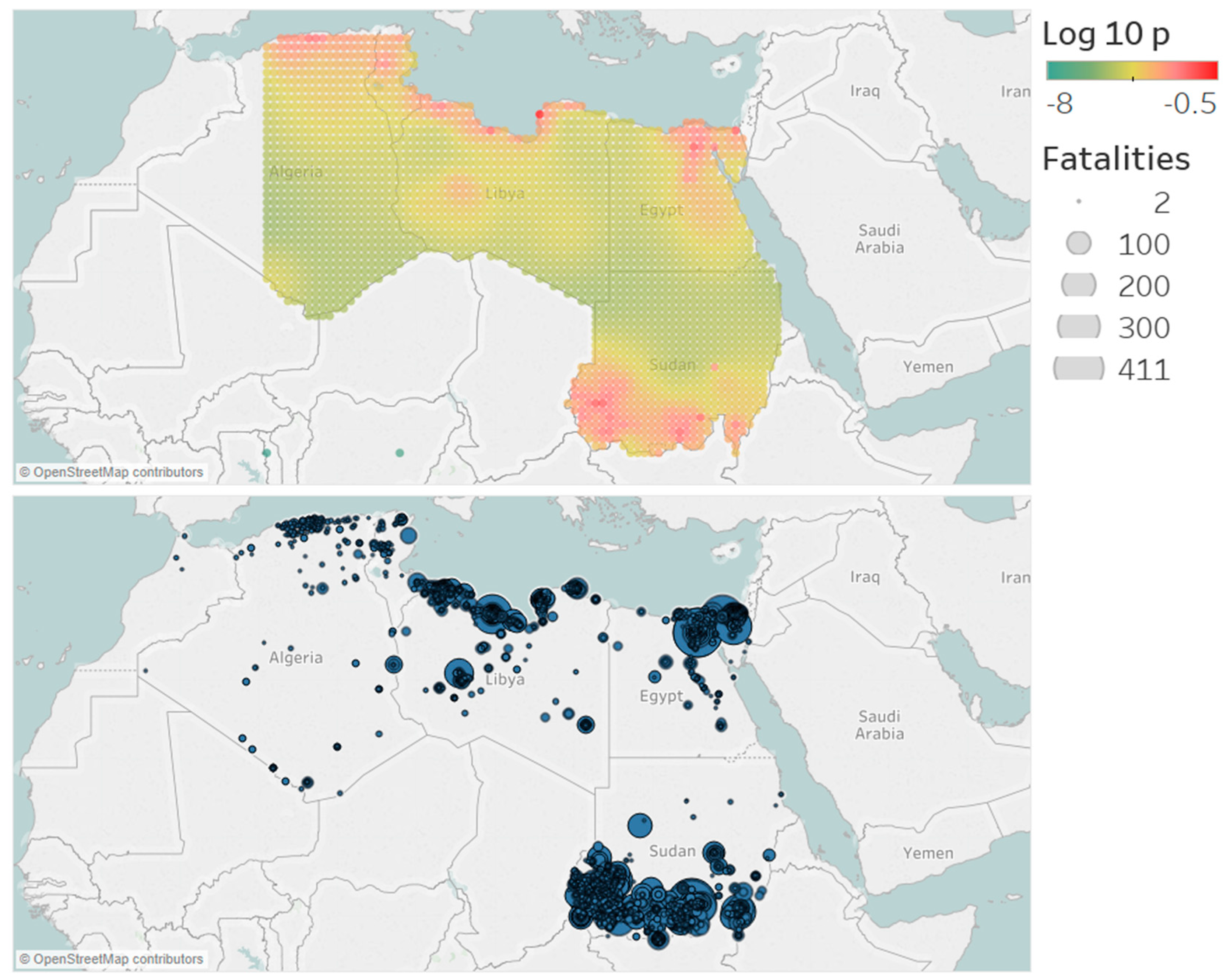
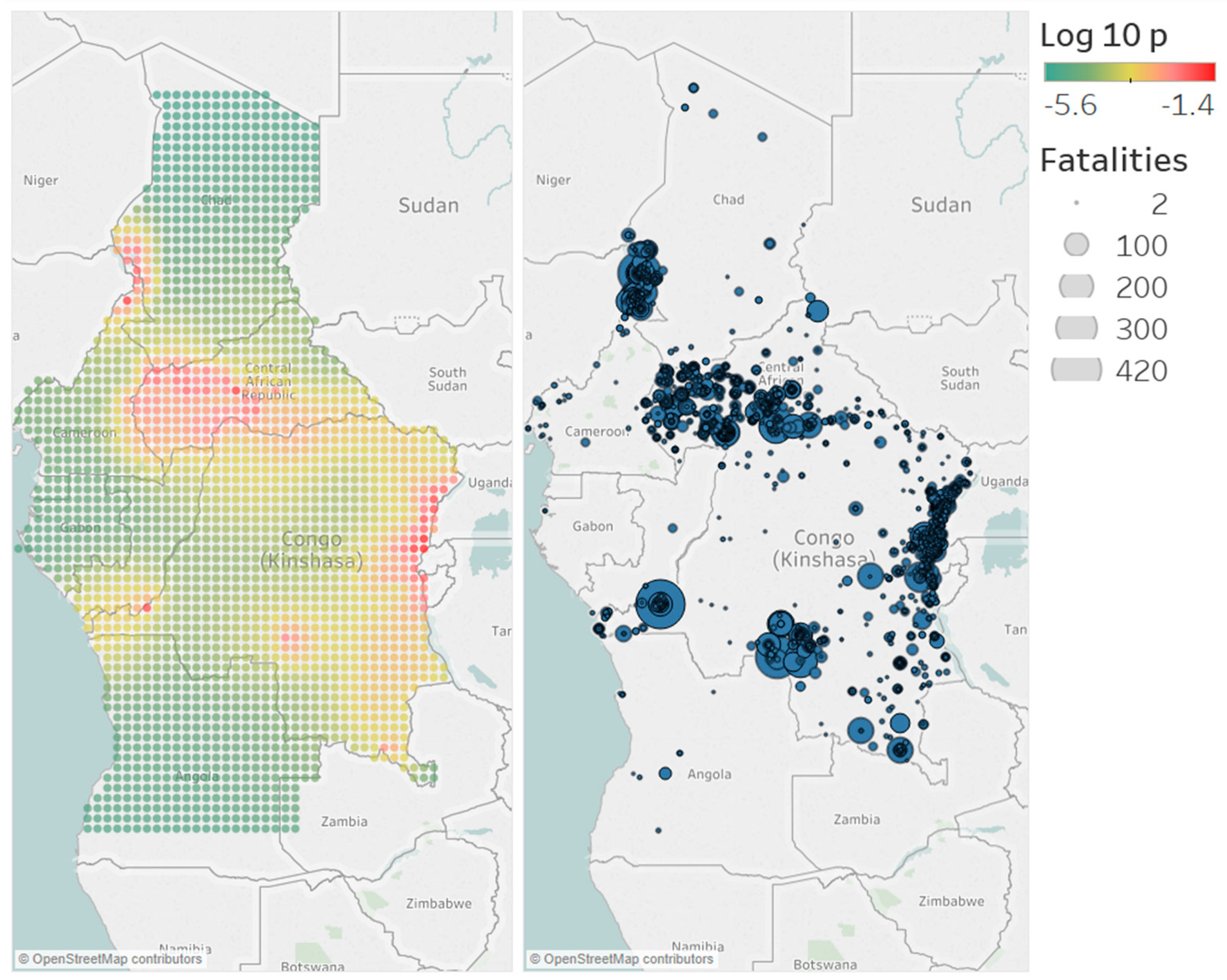
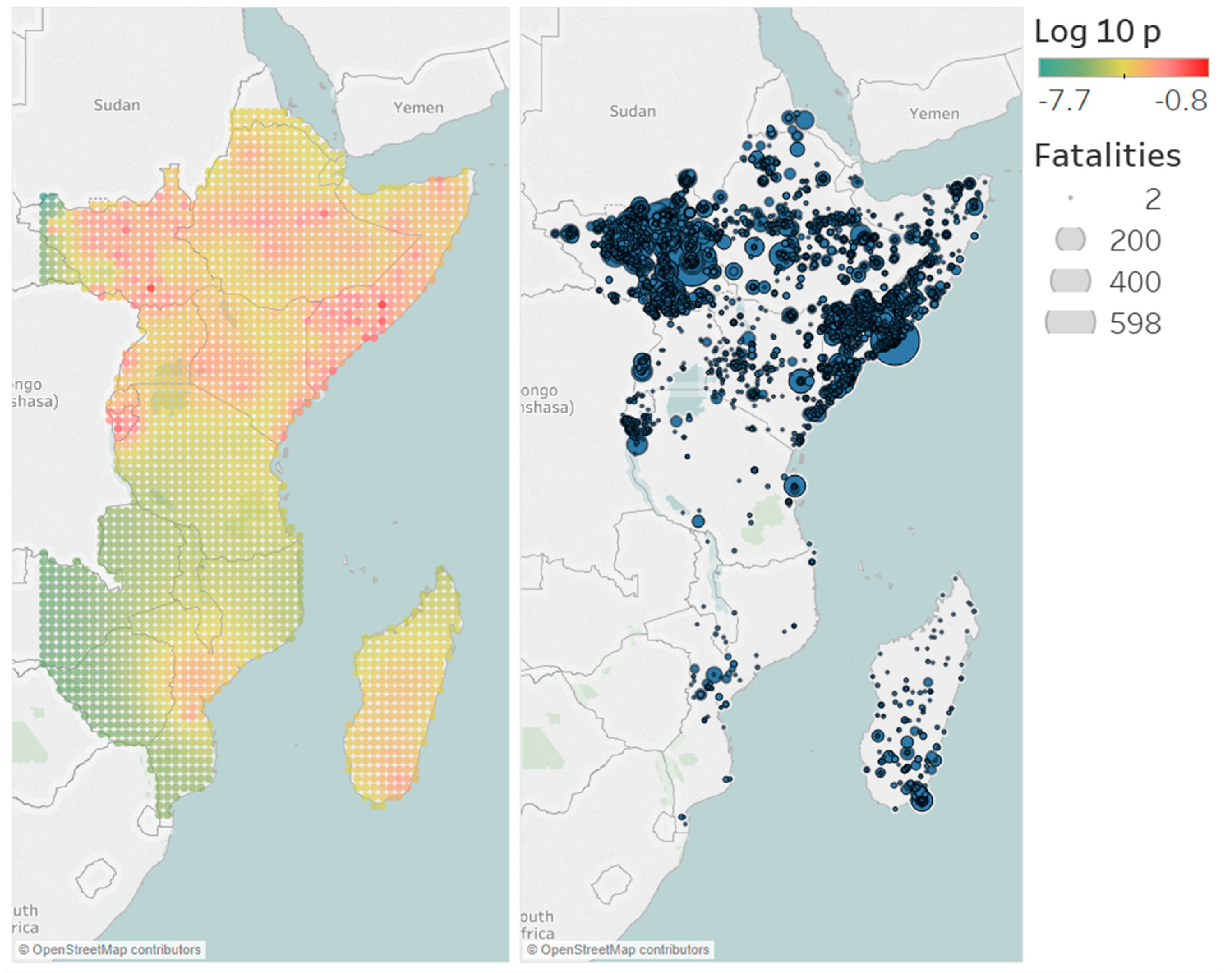
For each region, the study area is determined by the smallest rectangular area covering all events. The spatial background distribution is estimated for this area. As this means that it can cover areas that are not in the study region, such as other countries or parts of the ocean, the cells outside the study region are removed. The effect on the total probability should be minimal, as these areas have a very low probability due to a lack of events. The estimated spatial background distributions are given in Figure 6, Figure 7, Figure 8 and Figure 9 for North, West, Central and East Africa, respectively. Furthermore, a map with the actual conflicts in each region is given adjacent to the map of the background distribution. We see that the estimated distributions are in line with what we would expect from the catalogs, as the areas with high probability correspond with areas with high event density.

4.1. Parameter Estimates

For each region we have estimated the eight parameters of the spatial-temporal ETAS model $N_{SIM}=100$ times. The results for the North, West, Central and East Africa catalog are given in

Table 7. Parameter estimates for North Africa. Estimation results for the eight parameters of the ETAS model, the log likelihood and the number of events for the North Africa conflict catalog. Estimates marked with a * are at, or very close to, their constraint values. The best estimate, that is, the estimate of the run with the highest log likelihood, is given for each parameter. Furthermore, the median and the 95% confidence intervals are given.

Parameter	Best Value	Median	95% Confidence Interval
$\mu$	4.60e-1	5.05e-1	{4.17e-1, 5.45e-1}
k	3.76e-2	3.58e-2	{2.57e-2, 6.13e-2}
p	7.46e-1	7.43e-1	{6.79e-1, 8.53e-1}
c	1.00e-5 *	1.04e-5	{1.00e-5, 9.91e-2}
$\alpha$	0.39e-1	2.48e-1	{5.21e-3, 5.37e-1}
d	1.00e-2 *	1.00e-2	{1.00e-2, 1.00e-2}
q	3.00e0 *	3.00e0	{2.98e0, 3.00e0}
$\gamma$	6.94e-4 *	3.05e-3	{1.58e-5, 9.04e-3}
LogL	1.33.e3	1.31e3	{6.36e2, 1.33e3}
Events	3.56e3	3.63e3	{3.35e3, 3.75e3}

,

Table 8. Parameter estimates for West Africa. Estimation results for the eight parameters of the ETAS model, the log likelihood and the number of events for the West Africa conflict catalog. Estimates marked with a * are at, or very close to, their constraint values. The best estimate, that is, the estimate of the run with the highest log likelihood, is given for each parameter. Furthermore, the median and the 95% confidence intervals are given.

Parameter	Best Value	Median	95% Confidence Interval
$\mu$	5.02e-1	5.21e-1	{4.13e-1, 5.40e-1}
k	2.26e-2	2.24e-2	{1.75e-2, 3.02e-2}
p	7.0e1-1	7.22e-1	{6.61e-1, 7.51e-1}
c	1.00e-5 *	1.04e-5	{1.00e-5, 1.15e-2}
$\alpha$	2.46e-1	4.76e-1	{4.45e-2, 5.62e-1}
d	1.00e-2 *	1.00e-2	{1.00e-2, 1.00e-2}
q	3.00e0 *	3.00e0	{2.98e0, 3.00e0}
$\gamma$	1.97-4 *	2.15e-3	{2.54e-5, 6.74e-3}
LogL	−6.16e3	−6.17e3	{−6.20e2, −6.16e3}
Events	2.16e3	2.26e3	{2.04e3, 2.31e3}

,

Table 9. Parameter estimates for Central Africa. Estimation results for the eight parameters of the ETAS model, the log likelihood and the number of events for the Central Africa conflict catalog. Estimates marked with a * are at, or very close to, their constraint values. The best estimate, that is, the estimate of the run with the highest log likelihood, is given for each parameter. Furthermore, the median and the 95% confidence intervals are given.

Parameter	Best Value	Median	95% Confidence Interval
$\mu$	3.79e-1	3.59e-1	{3.01e-1, 4.34e-1}
k	3.52e-2	3.80e-2	{2.02e-2, 4.29e-2}
p	7.95e-1	7.96e-1	{7.48e-1, 8.28e-1}
c	1.00e-5 *	1.00e-5	{1.00e-5, 1.15e-2}
$\alpha$	3.03e-1	1.86e-1	{4.49e-2, 8.27e-1}
d	1.00e-2 *	1.00e-2	{1.00e-2, 1.00e-2}
q	3.00e0 *	2.99e0	{2.96e0, 3.00e0}
$\gamma$	3.21-5 *	5.65e-3	{8.02e-5, 2.39e-2}
LogL	−3.13e3	−3.15e3	{−3.30e2, −3.13e3}
Events	1.89e3	1.90e3	{1.68e3, 2.00e3}

and

Table 10. Parameter estimates for East Africa. Estimation results for the 8 parameters of the ETAS model, the log likelihood and the number of events for the East Africa conflict catalog. Estimates marked with a * are at, or very close to, their constraint values. The best estimate, that is, the estimate of the run with the highest log likelihood, is given for each parameter. Furthermore, the median and the 95% confidence intervals are given.

Parameter	Best Value	Median	95% Confidence Interval
$\mu$	8.38e-1	8.54e-1	{7.69e-1, 9.56e-1}
k	3.07e-2	2.96e-2	{2.25e-2, 3.88e-2}
p	7.14e-1	6.95e-1	{6.56e-1, 7.80e-1}
c	1.00e-5 *	1.05e-5	{1.00e-5, 1.19e-5}
$\alpha$	8.93e-2	6.13e-1	{1.09e-2, 5.29e-1}
d	1.00e-2 *	1.00e-2	{1.00e-2, 1.00e-2}
q	3.00e0 *	3.00e0	{2.97e0, 3.00e0}
$\gamma$	8.18-5 *	6.57e-3	{8.18e-5, 1.50e-2}
LogL	−8.39e3	−8.42e3	{−3.30e2, -3.13e3}
Events	4.59e3	4.68e3	{1.68e3, 2.00e3}

, and, respectively. In these tables, the parameter estimates of the best model, their median and distributions are given. Estimates with an * are estimates that are on, or are very close to, the boundary of their constraint. We see that this is the case for the parameters c, d, q and $\gamma$ in each region, where parameters c, d, and $\gamma$ go to their lower bound and q goes to its upper bound. The parameter c measures the incompleteness of the catalogs after a large event. As the conflicts in our database are reported on a daily basis, the next triggered event occurs the next day or later. It therefore makes sense that there are no undetected aftershocks right after an event. Furthermore, a value of $c=0$ would not much change the shape of the likelihood function. The term $d^2·\exp \left[2\gamma \left(M_i-M_c\right)\right]$ measures the influence of the magnitude on the spatial extent of the aftershock region for event i. As d goes to its lower bound and $\gamma$ tends to become arbitrarily small, it suggests that the magnitude has little influence on the region of aftershocks. If we decrease the lower bound of the constraint for parameter d it also tends to become arbitrarily small. In that case, the only influence on the spatial decay is the distance from the event.

The other parameters, $\mu ,$k, p, and $\alpha$ vary across the regions. For easy comparison, they are displayed together in

Table 11. Parameter estimates for the parameters $\mu$, k, p and $\alpha$ of the ETAS model. The values are the values from the ‘Best Value’ columns in Table 7, Table 8, Table 9 and Table 10. The last column gives the number of events in the study period.

Region	$\mathit{\mu }$	k	p	$\mathit{\alpha }$	Events
North	0.460	0.0376	0.746	0.139	3518
West	0.502	0.0226	0.701	0.246	2164
Central	0.379	0.0352	0.795	0.303	1834
East	0.838	0.0307	0.714	0.0893	4617

. What is most noticeable is that $p<1$ in the four regions. This implies that the process is explosive: each event generates an infinite number of triggered events when $t\to \infty$. However, this effect is not obvious from the data due to the short time span.

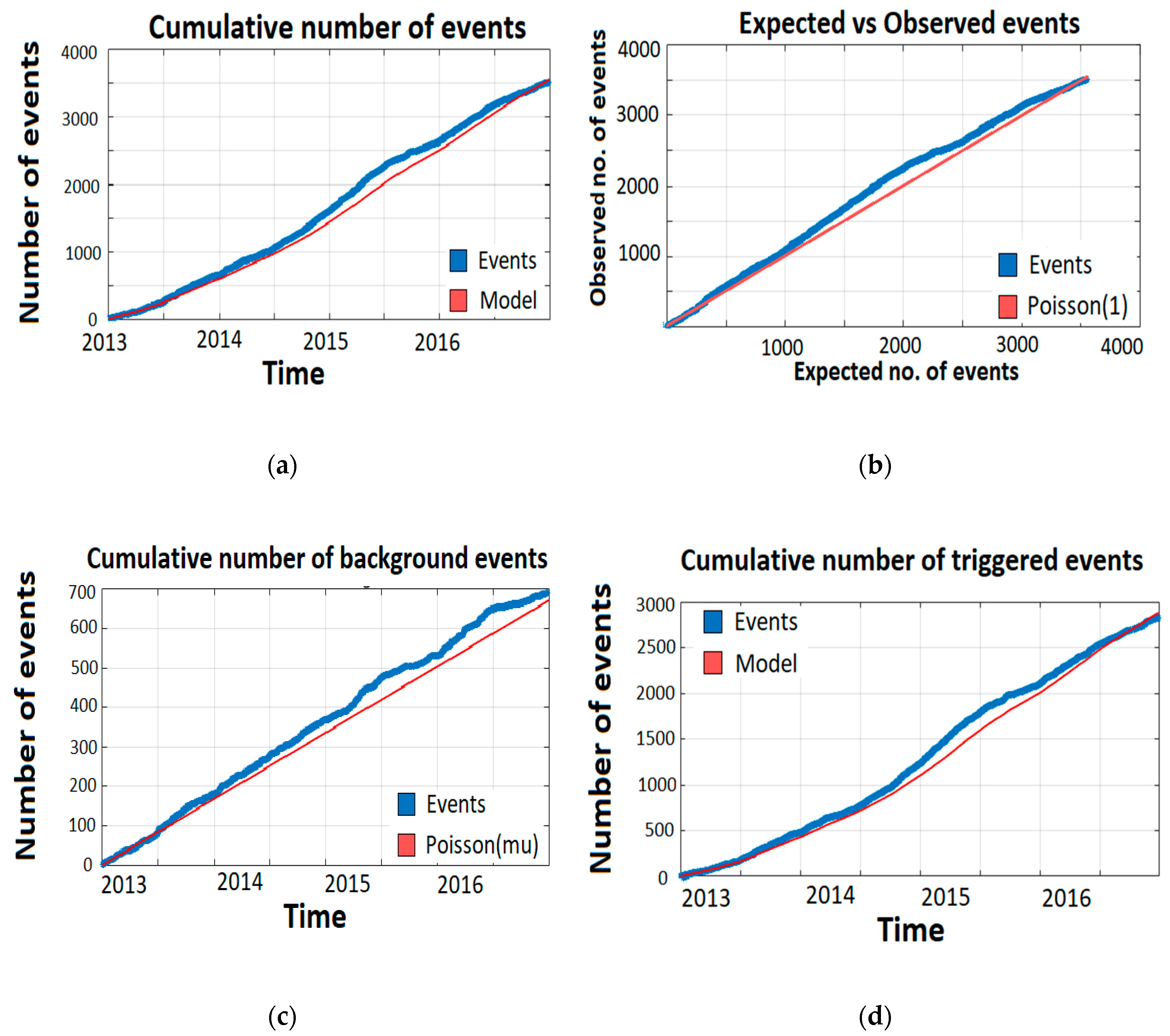
The value for the background rate $\mu$ in each region corresponds to the number of background events, which is given in

Table 12. Total number of expected and observed events, background events and triggered events for each region. The expected numbers of events are calculated using (12) to (14).

Region	All		Background		Triggered
	Expected	Observed	Expected	Observed	Expected	Observed
North	3558	3516	671	691	2887	2824
West	2160	2163	733	705	1427	1457
Central	1889	1834	553	525	1337	1308
East	4589	4616	1223	1255	3365	3361

. The numbers of expected and observed events are very close, which indicates that the model describes the data well. These expected and observed numbers are given over time in Figure 10 for North Africa. Results for the other three regions are very similar. When we divide the number of background events by the number of days, we obtain an average of 0.47, 0.48, 0.36 and 0.86 background events per day for the regions North, West, Central and East, respectively. Hence, the estimates for $\mu$ resemble the number of background events in the catalog.

The parameter k governs the expected number of direct aftershocks caused by an event. The estimation results in Table 11 suggest that events cause the most aftershocks in the North region (k = 0.0376) and the least in the West region (k = 0.0226). The parameter $\alpha$ measures the effect of magnitude in generating aftershocks. A small value indicates that the triggering rate is less dependent on magnitude. Hence, smaller events can trigger a larger amount of events more easily if $\alpha$ is small, see [8]. This suggests that in the East region (α = 0.0893) small conflicts can trigger larger amount of conflicts easier as compared to the other three regions.

4.2. Residuals

Figure 10 shows that the transformed event times, using (11), seem to follow a Poisson process with unit rate. In the bottom two figures, we see that this is also the case for background and triggered events. This suggests that the model is able to capture the temporal behavior of the process.

Whether the model captures the temporal behavior of the process can be tested more formally using the KS-test and the runs test. For each region, the null hypothesis that the inter-event times are exponentially distributed is rejected at the 1% level. This suggests that the model does not perfectly capture the temporal behavior of the process. In contrast, the runs test fails to reject the null hypothesis at the 1% level that the inter-event times are stationary and not autocorrelated.

4.3. Further Results

The results of the Number of Events tests are given in

Table 13. Results for the Number of Events’ test for the different regions. The estimated ETAS model for each region is used to simulate $N_{SIM}=100$ catalogs. The median and 95% confidence interval are calculated for the simulated catalogs, as well as the relative difference (% dif.). Furthermore, the probability (Prob.) that we observe the number of events in the event catalog or more events is in the final column.

Region	Median	Observed	% Dif.	95% Confidence Interval	Prob.
North	3101	3516	−11.8%	{2737, 3592}	0.064
West	1933	2163	−10.6%	{1774, 2107}	0.019
Central	1861	1834	+1.5%	{1652, 2076}	0.62
East	4506	4616	−2.4%	{4090, 4852}	0.34

. For each region, the median number of events and 95% confidence interval are given for the $N_{SIM}=100$ simulated catalogs based on the estimated ETAS model, as described above. Furthermore, the number of events in the conflict catalog is given, together with the probability that we observe a number of events larger than the number in the conflict catalog. We see that for the regions North, Central and East, the number of events in the conflict catalog lies within the 95% confidence bounds. For the West region the actually observed number of events is larger than expected by the model.

4.4. Forecasting for 2017

For the forecasts we simulated $N_{SIM}=100$ catalogs and calculated the median expected number of events in each cell in the year 2017. The total forecast can then be calculated as the sum over all cells. We only forecast large events, which are events with magnitude $M\ge 4$. This corresponds to events with 22 fatalities or more. The forecasts for each region are given in

Table 14. Forecasts for the number of events with magnitude $M\ge 4$ in 2017. The average number of these events in the period 2012–2016 is given, the number in 2016, the number predicted by the model and the observed number of events in 2017.

Region	Average	Last Year	Model	Observed
North	54.2	58	16.7	17
West	61.8	39	18.3	22
Central	23.2	13	13.8	39
East	58.4	50	30.5	69

. The forecasts are compared with two naive forecasts and the observed number of events. For the first naive forecast we use the average number of events in the period 2012–2016 and for the second naive forecast we use the number of large events of last year. We see that for the regions North and West, our ETAS based forecasts are much more accurate than the naive forecasts. In the Central and East region, our prediction underestimates the number of large events.

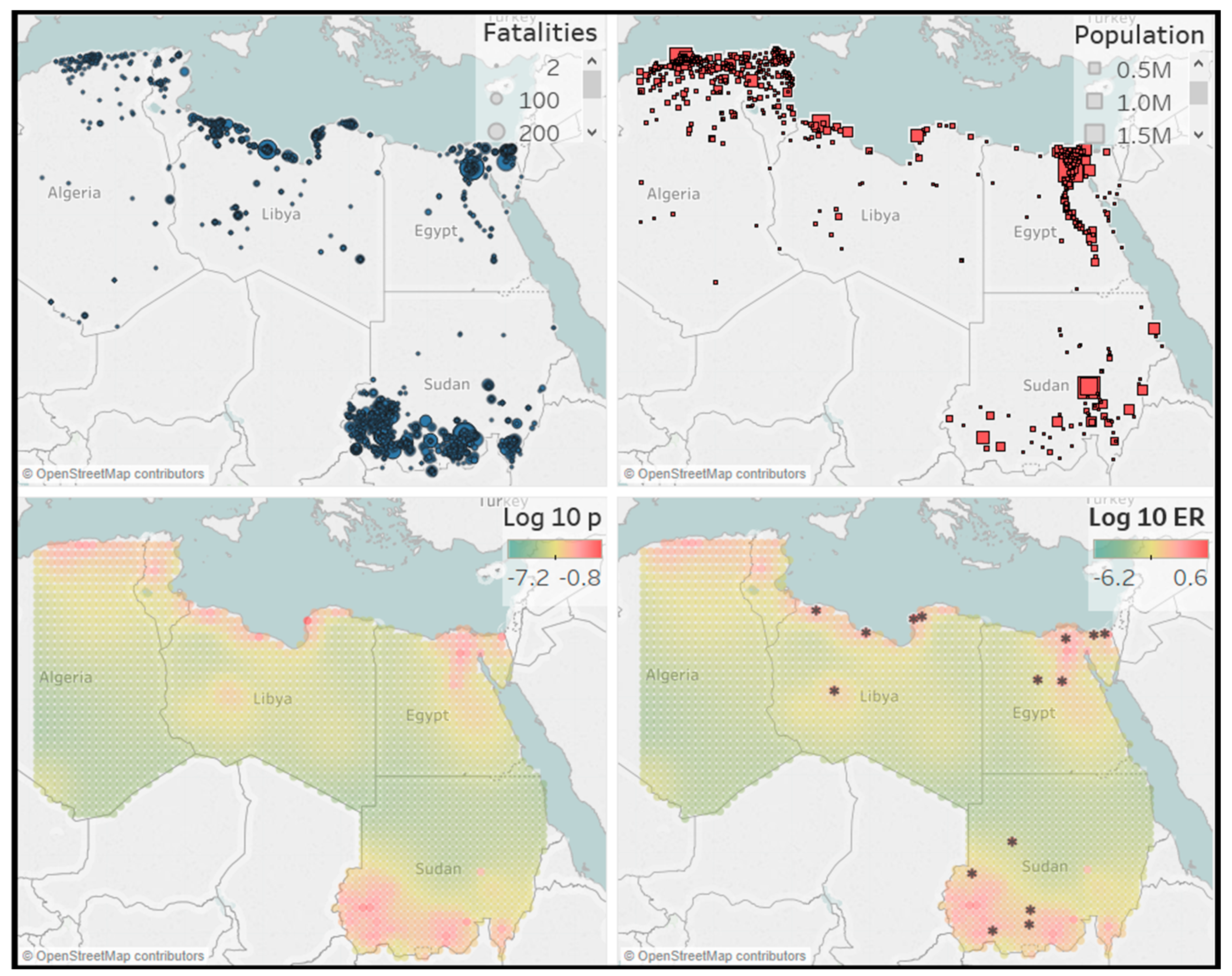
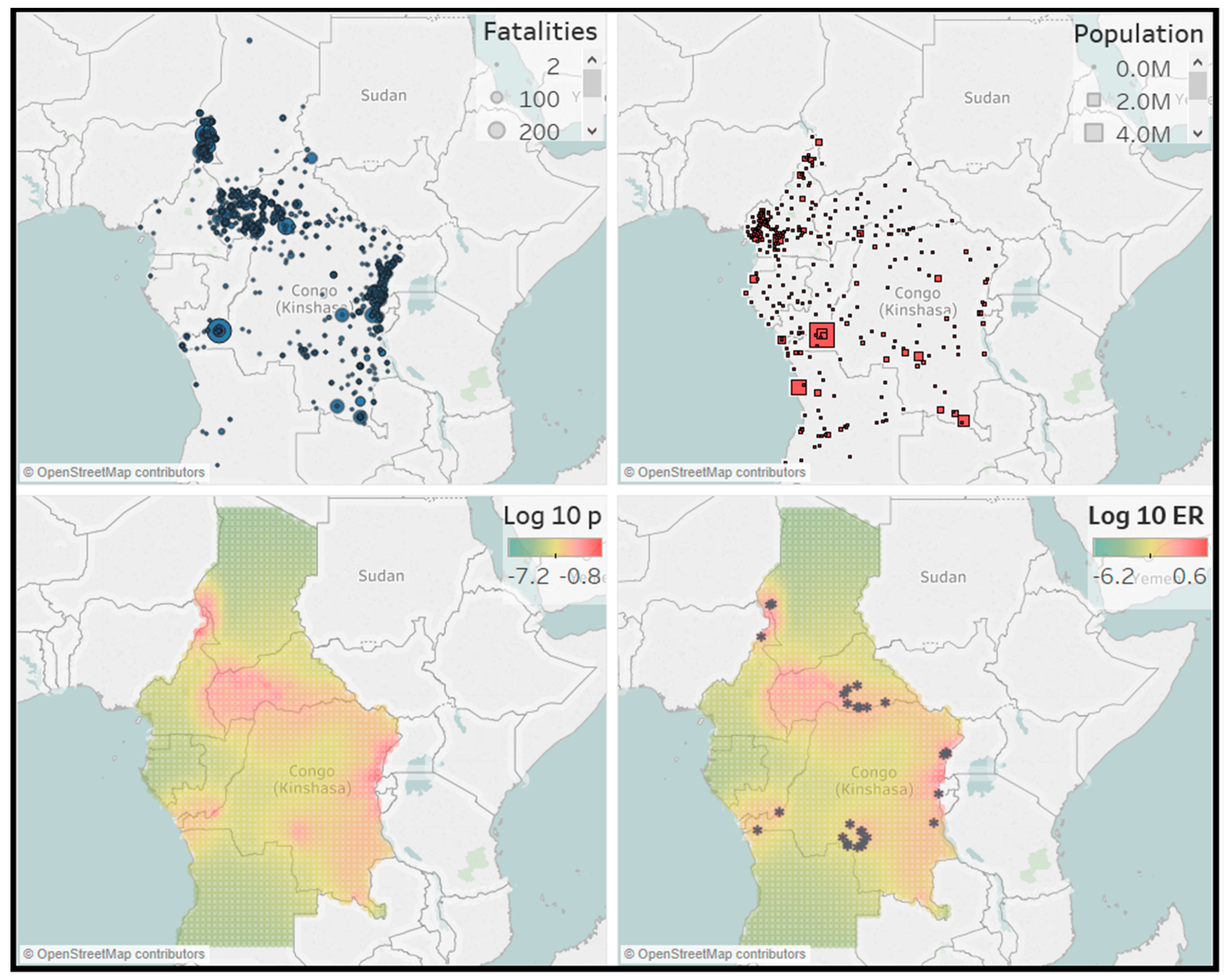
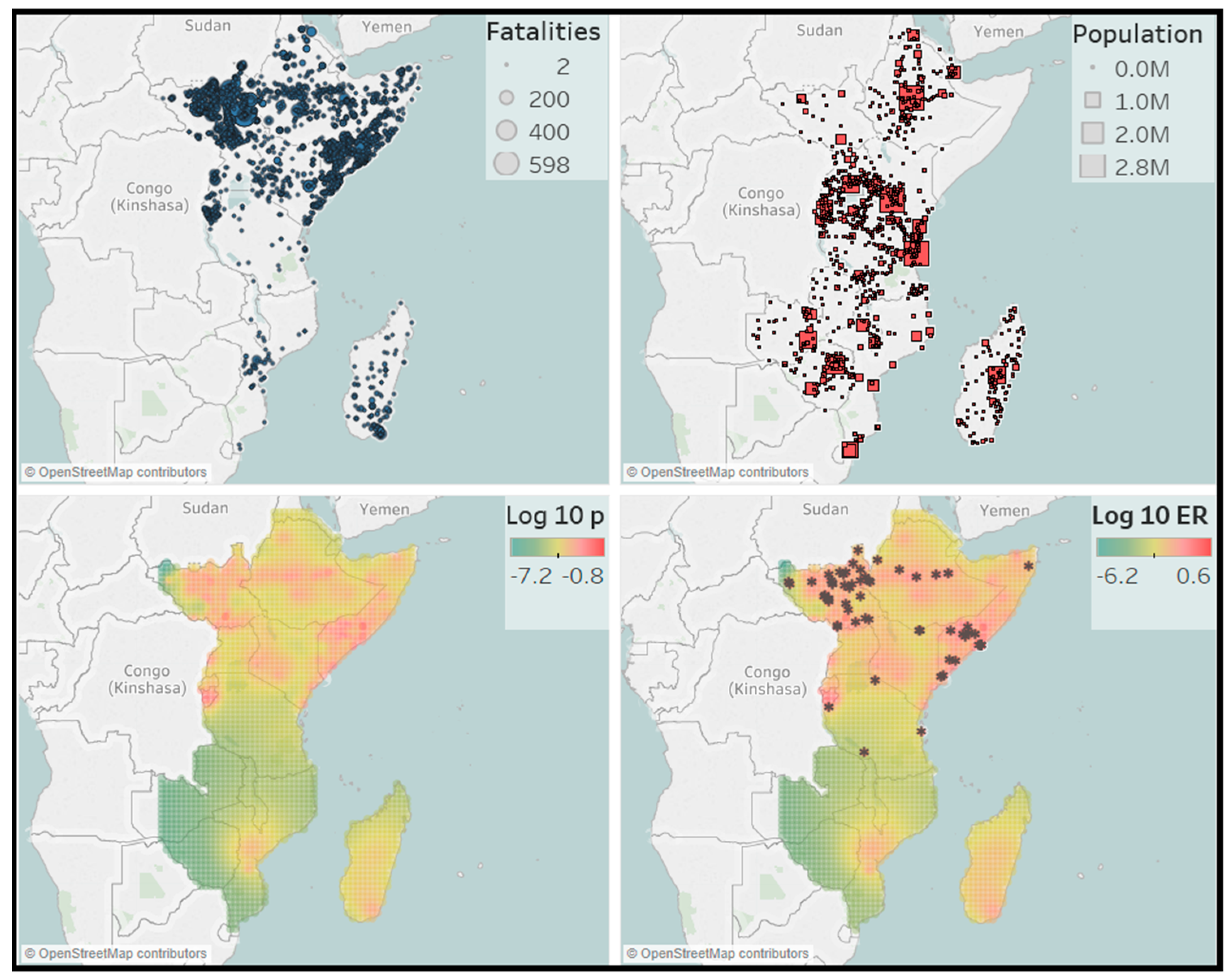
The results for the forecast locations of events is given in Figure 11, Figure 12, Figure 13 and Figure 14. For forecasting of event locations, we consider three other predictions for comparison. Two of them are naive predictions. We predict that future events happen at places where past events have happened and we predict that future events happen in highly populated areas or around country borders. For this, a map with the events is displayed, together with a map that shows every city with a population larger than 1000. The country borders can also be seen on this map. The third other prediction is based on our model and is the estimated spatial background distribution. This predicts that future events will happen at places where there is a high probability of background events. These three maps are displayed together with our forecasts map. The forecast map also includes the actual locations of the large events, indicated by an *.

First, we notice for the various graphs that there is little connection between population density and conflict areas. This can for example be seen in the West catalog where most conflicts take place in the north-east part of Nigeria or in the East catalog where most conflicts occur in South Sudan. The locations of previous conflict do seem to be a good predictor for future events. For our forecasts map, the similarity with the spatial background distribution is noticeable. A more detailed look reveals that each cell in the forecasting map is highly correlated with its equivalent cell in the background distribution. One explanation could be that, as the parameter $p<1$, the process becomes explosive and the simulations for the forecasting period are not accurate. Nonetheless, we believe that our forecasts maps are good predictors of the actual locations of future large events.

On average, the forecasts coincide with the locations in the event catalogs. There are also some areas in which our model is extra informative. These are regions with relatively few or small events in the past, but still show a high expected number in the future. For example, in the North catalog, we would not expect a future event in the center of Libya, as the previous events at that place were relatively small. Other such regions can be found in the West catalog, where two events in the west of Nigeria occurred. Finally, one of the clearest examples is in the Central catalog. In the forecast map, there is a cluster of large conflicts in an area of high intensity in the south of the Democratic Republic of the Congo. This was not expected from the event map, where only a few small events can be seen. Hence, even though the forecasting map is highly correlated with the spatial background distribution, it does produce useful predictions for the locations of future large events.

5. Conclusions and Further Research

We have estimated a spatial-temporal ETAS model on social conflict data in Africa. Using this model, we could make an out-of-sample forecast for the number of large future events and their locations. The estimated spatial background distribution showed that the probability distribution of background events was in line with the locations in the conflict catalogs, that is, high probability areas were associated with high event density areas. The Number of Events’ test showed that for three out of four regions, the number of events in the conflict catalog were close to the number of events expected by the model. Only for the West region the number of events was slightly underestimated. The KS-test showed that the inter-event times were not exactly exponentially distributed, and this indicated that the model does not perfectly capture the temporal behavior of the data. The runs test however suggested that the inter-event times are stationary and not autocorrelated.

We were able to use the estimated model to make predictions for the number and locations of future large events, out-of-sample. The forecast locations were in line with the locations of actual events.

Limitations and Future Research

The ETAS model and estimation procedures have been optimized specifically for estimating earthquake catalogs, and our study is the first to bring it to social conflict data. We used the constants for the cooling procedure, and it seemed to work reasonably well. This, however, does not mean that these are the optimal constants for estimating conflict catalogs. Moreover, the parameter constraints in estimating the model are obtained from the earthquake literature and these might be too strict for modeling conflicts. However, when we relaxed these constraints, we ran into estimation problems, as some parameters became arbitrarily small or large. This problem persisted after much trial and error with different constraint values. Hence, further research into the estimation procedure and parameter constraints regarding social conflicts might produce better results. It may also be that the parameter constraints are one of the causes of forecast failure for some of the regions. More experience with those constraints and their impact on forecast accuracy is mandatory.

The model estimated in this study is the stationary ETAS model, which assumes that the background rate does not change over time. This is not always the case for conflict data. For example, the rise of the Arab Spring in North Africa caused a stream of events. Our study can perhaps be extended using a non-stationary ETAS model as in [8], where the background rate varies over time. Furthermore, the models for earthquakes work with continuous time, while the conflicts are only reported with a daily precision. Another possible extension might therefore be a discrete time implementation. Finally, the model used in this study assumed the Gutenberg–Richter law for the magnitude distribution, as it closely resembles the magnitude distribution of earthquakes. One could consider a different distribution that is more natural to the size distribution of conflicts.

Regarding the data, it would be interesting to consider our model to smaller regions. Regions of interest could be the north-east of Nigeria, where the Boko Haram insurgency is active, the conflicts around Lake Chad or around the Sudan South-Sudan border. Our study focused more on aggregate conflict dynamics and it would be interesting to see if the findings hold at a smaller scale.

References

- Beck, N.; King, G.; Zeng, L. Improving quantitative studies of international conflict: A conjecture. Am. Political Sci. Rev. 2000, 94, 21–35. [Google Scholar] [CrossRef] [Green Version]
- Cederman, L.-E.; Weidmann, N.B. Predicting armed conflict: Time to adjust our expectations? Science 2017, 355, 474–476. [Google Scholar] [CrossRef] [PubMed] [Green Version]
- Chadefaux, T. Conflict forecasting and its limits. Data Sci. 2017, 1, 7–17. [Google Scholar] [CrossRef] [Green Version]
- Goldstone, J.A.; Bates, R.H.; Epstein, D.L.; Gurr, T.R.; Lustik, M.B.; Marshall, M.G.; Ulfelder, J.; Woodward, M. A global model for forecasting political instability. Am. J. Political Sci. 2010, 54, 190–208. [Google Scholar] [CrossRef]
- Colaresi, M.; Mahmood, Z. Do the robot: Lessons from machine learning to improve conflict forecasting. J. Peace Res. 2017, 54, 193–214. [Google Scholar] [CrossRef]
- Ettensperger, F. Comparing supervised learning algorithms and artificial neural networks for conflict prediction: Performance and applicability of deep learning in the field. Qual. Quant. 2019, 54, 567–601. [Google Scholar] [CrossRef]
- Hudson, V.M.; Schrodt, P.A.; Whitmer, R.D. Discrete sequence rule models as a social science methodology: An exploratory analysis of foreign policy rule enactment within Palestinian–Israeli event data. Foreign Policy Anal. 2008, 4, 105–126. [Google Scholar] [CrossRef]
- Lombardi, A.M. SEDA: A software package for the statistical earthquake data analysis. Sci. Rep. 2017, 7, 44171. [Google Scholar] [CrossRef] [PubMed] [Green Version]
- Ogata, Y. Statistical models for earthquake occurrences and residual analysis for point processes. J. Am. Stat. Assoc. 1988, 83, 9–27. [Google Scholar] [CrossRef]
- Ogata, Y. Space-time point-process models for earthquake occurrences. Ann. Inst. Stat. Math. 1998, 50, 379–402. [Google Scholar] [CrossRef]
- Zhuang, J.; Ogata, Y.; Vere-Jones, D. Stochastic declustering of space-time earthquake occurrences. J. Am. Stat. Assoc. 2002, 97, 369–380. [Google Scholar] [CrossRef]
- Kumazawa, T.; Ogata, Y. Nonstationary ETAS models for nonstandard earthquakes. Ann. Appl. Stat. 2014, 8, 1825–1852. [Google Scholar] [CrossRef]
- Sen, M.K.; Stoffa, P.L. Global Optimization Methods in Geophysical Inversion; Cambridge University Press (CUP): Cambridge, UK, 2013. [Google Scholar]
- Van den Hengel, G. An Epidemic Type Aftershock Sequence model on Conflict Data in Africa, Unpublished. Master’s Thesis, Econometric Institute, Erasmus School of Economics, Rotterdam, The Netherlands, 2018. [Google Scholar]
- Lin, F.-T.; Kao, C.-Y.; Hsu, C.-C. Applying the genetic approach to simulated annealing in solving some NP-hard problems. IEEE Trans. Syst. Man Cybern. 1993, 23, 1752–1767. [Google Scholar] [CrossRef]
- Lombardi, A.M. Estimation of the parameters of ETAS models by Simulated Annealing. Sci. Rep. 2015, 5, 8417. [Google Scholar] [CrossRef] [PubMed] [Green Version]
Figure 1.
Cumulative number of events and fatalities over time.
Figure 2.
Map of social conflicts in Africa in the period 2012–2017 with at least two fatalities. Events with more than 100 fatalities are colored red.
Figure 3.
The latitude and longitude of events over time. The red lines represent the latitude and longitude of the geographical center of Africa. In the latitude plot, points above the red line are more north and points below are more south. In the longitude plot, points above the red line are more east and points below the red line are more west.
Figure 4.
Distribution of the number of events. The blue bars in the top figure show the number of events for each magnitude and the red line is the number of events corresponding to the Gutenberg–Richter law. In the bottom figure, the logarithm base 10 of the same data is shown. If the magnitude distribution follows the Gutenberg–Richter law, the blue bars in the bottom figure should correspond to the red line.
Figure 5.
The five major regions of Africa: North, West, Central, East and South. Source: Wikimedia Commons, the free media repository.
Figure 6.
Spatial background distributions of the model with the largest log-likelihood for the region North Africa. The area is divided into cells. In these cells, the background intensity is assumed to be homogeneous. The cells give the probability of a background event occurring in that cell.
Figure 7.
Spatial background distributions of the model with the largest log-likelihood for the region West Africa. The area is divided into cells. In these cells, the background intensity is assumed to be homogeneous. The cells give the probability of a background event occurring in that cell.
Figure 8.
Spatial background distributions of the model with the largest log-likelihood for the region Central Africa. The area is divided into cells. In these cells, the background intensity is assumed to be homogeneous. The cells give the probability of a background event occurring in that cell.
Figure 9.
Spatial background distributions of the model with the largest log-likelihood for the region East Africa. The area is divided into cells. In these cells, the background intensity is assumed to be homogeneous. The cells give the probability of a background event occurring in that cell.
Figure 10.
Results of the residual analysis for the North Africa catalog. In the top left (a) figure the observed number of events is plotted against the transformed times from (11). In the top right figure (b), the observed number of events (blue) is plotted against the expected number of events by the model (red). In the bottom two figures (c) and (d), the observed number of background and triggered events (blue) are compared with the number of events expected by the model (red).
Figure 11.
Forecasts for North Africa. Top left: event catalog 2012–2016. Top right: City map with cities with 1000+ population. Bottom left: spatial background distribution estimated from the data from 2012–2016. Bottom right: forecast for the expected number of events with in each cell in the year 2017, together with the locations of the actual conflicts that have taken place with .
Figure 12.
Forecasts for West Africa. Top left: event catalog 2012–2016. Top right: City map with cities with 1000+ population. Bottom left: spatial background distribution estimated from the data from 2012–2016. Bottom right: forecast for the expected number of events with in each cell in the year 2017, together with the locations of the actual conflicts that have taken place with .
Figure 13.
Forecasts for Central Africa. Top left: event catalog 2012–2016. Top right: City map with cities with 1000+ population. Bottom left: spatial background distribution estimated from the data from 2012–2016. Bottom right: forecast for the expected number of events with in each cell in the year 2017, together with the locations of the actual conflicts that have taken place with .
Figure 14.
Forecasts for East Africa. Top left: event catalog 2012–2016. Top right: City map with cities with 1000+ population. Bottom left: spatial background distribution estimated from the data from 2012–2016. Bottom right: forecast for the expected number of events with in each cell in the year 2017, together with the locations of the actual conflicts that have taken place with .