Mean Field Bias-Aware State Updating via Variational Assimilation of Streamflow into Distributed Hydrologic Models

Abstract

When there exist catchment-wide biases in the distributed hydrologic model states, state updating based on streamflow assimilation at the catchment outlet tends to over- and under-adjust model states close to and away from the outlet, respectively. This is due to the greater sensitivity of the simulated outlet flow to the model states that are located more closely to the outlet in the hydraulic sense, and the subsequent overcompensation of the states in the more influential grid boxes to make up for the larger scale bias. In this work, we describe Mean Field Bias (MFB)-aware variational (VAR) assimilation, or MVAR, to address the above. MVAR performs bi-scale state updating of the distributed hydrologic model using streamflow observations in which MFB in the model states are first corrected at the catchment scale before the resulting states are adjusted at the grid box scale. We comparatively evaluate MVAR with conventional VAR based on streamflow assimilation into the distributed Sacramento Soil Moisture Accounting model for a headwater catchment. Compared to VAR, MVAR adjusts model states at remote cells by larger margins and reduces the Mean Squared Error of streamflow analysis by 2–8% at the outlet Tiff City, and by 1–10% at the interior location Lanagan.

1. Introduction

Streamflow observations are used extensively to update hydrologic model states via various forms of data assimilation (DA) [1,2,3,4,5,6,7,8,9,10,11,12]. Assimilating streamflow data into distributed models compared to that into lumped models presents additional challenges due to the greatly increased dimensionality of the inverse problem as elaborated below. In distributed modeling, changes in model states at a cell distant from a high-order stream exert a much smaller influence on the model-simulated flow at the catchment outlet compared to those at a cell near a high-order stream. This is because the runoff generated near a low-order stream, that is, in a headwater area, has to travel much longer distances to reach a high-order stream where channel flow takes over. Most of the above travel occurs on hillslopes where the flow is greatly attenuated. Unlike channel flow, hillslope flow occurs through numerous flow paths on the land surface and pore spaces in the subsurface. These flow paths vary greatly in size, length and shape, and have much larger friction factors than channels. Compared to channel flow, hillslope flow is hence subject to mechanical dispersion and is characterized by smaller ratios of advective to diffusive transport [13]. Recall in the advection-diffusion solution [14,15] that the width of a pulse inflow varies approximately with $\sqrt{\mathrm{Dt}}$ where $\mathrm{D}$ and $\mathrm{t}$ denote the diffusivity and time elapsed, respectively. Larger $\mathrm{D}$ and $\mathrm{t}$ due to dispersion and longer travel time mean that hillslope flow is greatly attenuated and that sensitivity of changes in runoff generation to lateral inflow into channels via hillslope routing is dampened out for DA to effectively source-trace. Consequently, the sensitivity of the model-simulated streamflow at the outlet to the changes in the model states is smoothed out in the upstream areas of the catchment. Most data assimilation (DA) methods use this spatiotemporal pattern of sensitivity for gradient-based minimization at the grid box scale whether it is evaluated via adjoint code as in variational assimilation (VAR, [16]) or estimated via random sampling in ensemble subspace as in ensemble Kalman filter (EnKF, [17]). The above observation indicates that, when there exist catchment-wide biases, DA at the grid box scale is likely to over- and under-adjust the model states close to and distant from high-order streams to compensate for the large-scale bias. The premise of this work is that one may improve the performance of DA significantly by updating the model states at the catchment scale first and then the resulting states at the grid box scale.

Correcting spatiotemporal biases such as MFB, local bias (LB) and conditional bias (CB) in the data or modeled variables has been extensively explored in statistical pre- and post-processing, calibration, and DA. Bias correction has also been shown to be effective in improving estimation and prediction of soil moisture [18,19], precipitation [20,21], streamflow [22] and extremes [23] as well as forecast models [24], and state updating [25]. In lumped hydrologic modeling, streamflow prediction is improved by correcting biases in forcing forecasts [26,27] or by accounting for CBs in model soil moisture [9]. Correcting MFB has been widely used in gridded precipitation analysis [28,29,30], which in turn improves streamflow prediction [11]. In distributed hydrologic modeling, correcting MFB in radar-based precipitation estimates improved streamflow and soil moisture [11]. In calibration, adjusting model parameters spatially uniformly also helps preserve their spatial structure [31]. While diverse bias correction methods have emerged in hydrology, correcting the MFB in states of a distributed hydrologic model is new and warrants the development of the MFB-aware DA framework and the assessment of its practicality.

In this work, we describe and evaluate MFB-aware VAR, referred to herein as MVAR, for state updating of distributed hydrologic models based on variational assimilation of streamflow data. MVAR adjusts the model states at the catchment scale first and adjusts the resulting states at the grid box scale. One may hence consider MVAR the simplest form of multiscale DA [32,33] employing two scales, that is, the entire catchment and a grid box. Catchment-wide adjustment in the first step mitigates over- and under-correction of model states at the grid box scale and helps preserve the spatial structure of the background states in the updated fields. Lee et al. [8] have shown that basin-wide uniform adjustment of model states is often able to produce flow predictions that are as accurate as those from adjusting states at individual cells. In such cases, the first step of MVAR would be the main contributor to DA performance and also limit the changes to the background states to a minimum. Note that, if two DA solutions have the same predictive skill, the one with smaller adjustments to the background states should be preferred [33,34]. The effectiveness of MVAR depends also on the goodness of the hydrologic models. If significant parametric or structural errors exist, they are likely to compromise the performance of MVAR. To assess the impact of model errors, we carry out an evaluation using both weakly- and strongly-constrained DA, the latter of which does not assume model errors. The significant new contributions of this paper are the development of MFB-aware DA for streamflow assimilation into the distributed model and the comparative analysis and evaluation of MVAR and VAR. This paper is organized as follows. Section 2 describes the hydrologic model used and the two assimilation approaches, that is, MVAR and VAR. Section 3 describes the study basin and evaluation metrics used. Section 4 and Section 5 present results and conclusions, respectively.

2. Model and Data Assimilation

Since the formulation of the assimilation problem is specific to the model used, we first describe the hydrologic model in Section 2.1, followed by formulating the problem in the case of MVAR and VAR in Section 2.2 and Section 2.3, respectively.

2.1. Hydrological Model

The model used is the distributed Sacramento Soil Moisture Accounting (SAC-SMA; [35]) included in the US National Weather Service Hydrology Laboratory’s Research Distributed Hydrologic Model [31]. The distributed SAC-SMA model operates on the Hydrologic Rainfall Analysis Project (HRAP; [36]) grid mesh of about 4 km in size where NWS radar and multisensor precipitation estimates are available. For potential evaporation, monthly climatology on the HRAP grid is used [7]. The SAC-SMA computes fast and slow runoff components from two subsurface storages, namely, the Upper Zone (UZ) and the Lower Zone (LZ) where the LZ is typically thicker than the UZ.

Table 1. Model states updated via MVAR and VAR for the distributed SAC-SMA model.

SAC-SMA Model States	Description
UZTWC	Upper Zone Tension Water Content
UZFWC	Upper Zone Free Water Content
LZTWC	Lower Zone Tension Water Content
LZPFC	Lower Zone Primary Free Water Content
LZSFC	Lower Zone Supplemental Free Water Content
ADIMC	Additional impervious area water content

summarizes tension (TWC) and free water contents (FWC) in the UZ and LZ.

Tension water contents (UZTWC and LZTWC) are related to soil moisture bounded to soil particles and free water contents (UZFWC, LZPFC, LZSFC) are related to soil gravitational water. Primary (LZPFC) and supplemental (LZSFC) free water contents in the LZ produce slow- or fast-responding baseflow, respectively. Tension and free soil moisture contents and the additional impervious area water content (ADIMC) interact with each other and generate baseflow, interflow, surface runoff, direct runoff, and impervious area runoff. The kinematic-wave routing model is then used to route the runoff through the hillslopes and channels based on cell-to-cell connectivity information created from the cell outlet tracing with an area threshold (COTAT) algorithm [31,37]. A priori parameters of the distributed SAC-SMA were estimated from the STATSGO2 soil data [38] and the routing parameters were from the digital elevation model (DEM) and channel hydraulic data [31]. This study used manually-optimized model parameters obtained from Phase 1 of the Distributed Model Intercomparison Project (DMIP, [39]). The soil moisture translation routine of the SAC-SMA with heat transfer dynamics (SAC-HT; [40]) is used to calculate depth-specific soil moisture contents from the original SAC-SMA model states.

2.2. MFB-Aware Variational Data Assimilation, MVAR

The following states the data assimilation problem solved in this study. Given the a priori model states, streamflow observations at either outlet or both outlet and interior locations, and observed precipitation (P) and monthly climatology of potential evapotranspiration (PE), update the distributed model soil moisture states at the beginning of the assimilation window and multiplicative biases in P and PE. The model may be applied as a weak constraint to this problem by considering model inadequacies [41,42,43].

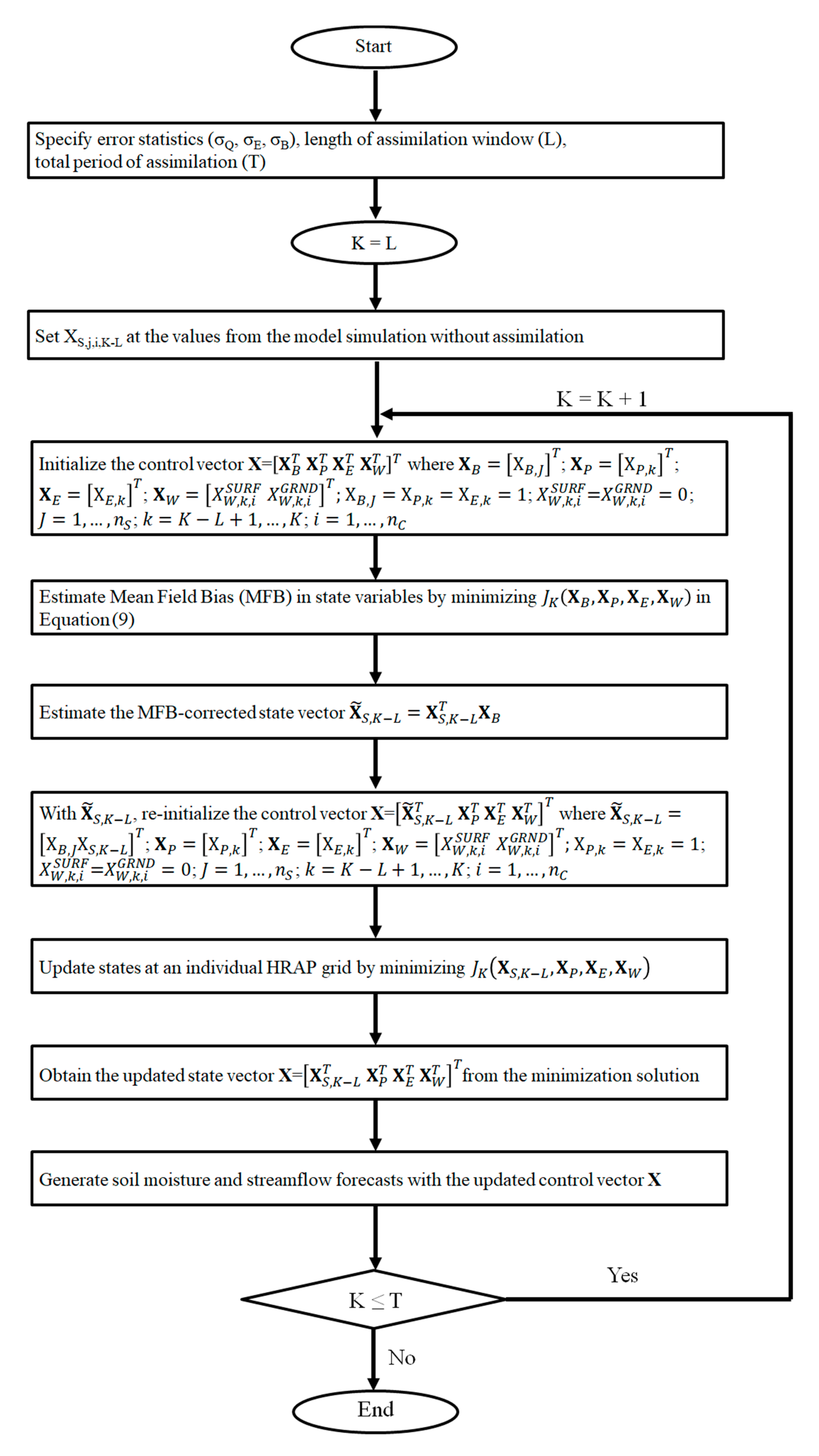
MVAR first adjusts model states via multiplying MFB estimates and then individually updates at the HRAP scale. With enough length of the assimilation window, the MFB estimate effectively affects interior points through propagating outlet flow information to upstream pixels via the routing process, not just affected by high sensitivity area around the basin outlet pixel. The two-step approach in estimating MFB and HRAP cell-scale errors is to reduce the dimensionality or ill-posedness of the assimilation problem. Similar examples include dual state-parameter estimation [44] or data assimilation by field alignment to solve separately displacements and amplitudes [45]. The MFB estimation step can be formulated as the nonlinear constrained least-squares minimization problem in Equations (1) and (2).

Minimize

$$\begin{gathered} J_K\left(X_B,X_P,X_E,X_W\right)=\frac{1}{2}{\left[Z_B-H_B{X}_B\right]}^T{R}_B^{-1}\left[Z_B-H_B{X}_B\right] \\ +\frac{1}{2}{\left[Z_P-H_P{X}_P\right]}^T{R}_P^{-1}\left[Z_P-H_P{X}_P\right] \\ +\frac{1}{2}{\left[Z_E-H_E{X}_E\right]}^T{R}_E^{-1}\left[Z_E-H_E{X}_E\right] \\ +\frac{1}{2}{\left[Z_Q-H_Q\left(X_{S,K-L},X_P,X_E,X_W\right)\right]}^T{R}_Q^{-1}\left[Z_Q-H_Q\left(X_{S,K-L},X_P,X_E,X_W\right)\right] \\ +\frac{1}{2}{X}_W{}^T{R}_W^{-1}{X}_W \end{gathered}$$

(1)

subject to

$$\{\begin{array}{c}{X}_{S,k}=\mathbf{M}\left(X_{S,k-1},X_P,X_E\right), k=K-L+1, \dots , K \\ X_{S,j,i}^{min}\le X_{S,j,i,k}\le X_{S,j,i}^{max}, k=K-L, \dots , K;j=1, \dots , n_S;i=1, \dots , n_C\end{array}$$

(2)

In Equation (1), $Z_B=X_{S,K-L}$ and $H_B=X_{S,K-L}^T$. $X_B={\left[X_{B,j}\right]}^T$ is the vector composed of MFB for individual model states where $j=1, \dots , n_S$; $J_K$ denotes the objective function value at hour K; $X_S$ denotes the state vector of the SAC-SMA model, or UZTWC, UZFWC, LZTWC, LZSFC, LZPFC, and ADIMC (Table 1); $X_{S,K-L}$ represents $X_S$ at the beginning ($k=K-L$) of the assimilation window, that is, background model states as driven by the base model simulation; $X_P$ and $X_E$ denote the multiplicative adjustment factors for the precipitation and Potential Evaporation (PE) data at $k=K-L+1, \dots , K$, respectively, within the assimilation window; the subscript $k$ denotes the time index; $X_{S,j,i}^{min}$ and $X_{S,j,i}^{max}$ denote the lower and upper bounds of the j-th state variable at the i-th grid, $X_{S,j,i}$; $n_S$ denotes the number of SAC states ($n_S$ = 6 in this study for both distributed and lumped SAC-SMA); $n_C$ denotes the number of HRAP cells within the basin; $L$ denotes the length of the assimilation window—the duration of the unit hydrograph is used for $L$ which represents the time scale of the fast response of the basin; $M()$ denotes the SAC-SMA model; $H_B$, $H_P$, $H_E$, and $H_Q()$ denote the observation operators that relate the control vector ($X_{S,K-L},X_P,X_E,X_W$) to observations ($Z_B$, $Z_P$, $Z_E$, $Z_Q$) where, in this study, $H_B=I$, $H_P=Z_P$, $H_E=Z_E$, and $H_Q()$ is the distributed SAC-SMA and kinematic-wave routing models; $R_B$, $R_P$, $R_E$, $R_Q$, and $R_W$ denote the measurement error covariance matrices for background model states, precipitation, PE, streamflow, and the model error, respectively; $Z_P$, $Z_E$, and $Z_Q$ denote the observations of precipitation, PE, and streamflow at $k=K-L+1, \dots , K$, respectively; Equation (1) is based on the following observation equations:

$$Z_B=H_B{X}_B+V_B$$

(3)

$$Z_P=H_P{X}_P+V_P$$

(4)

$$Z_E=H_E{X}_E+V_E$$

(5)

$$Z_Q=H_Q\left(X_{S,K-L},X_P,X_E,X_W\right)+V_Q$$

(6)

$$Z_W=H_W\left(X_{S,K-L},X_P,X_E,X_W\right)+V_W$$

(7)

In the above, $V_B$, $V_P$, $V_E$, $V_Q$, and $V_W$ denote measurement error vectors for background model states, precipitation, PE, streamflow, and the rainfall-runoff model error. The Z_W denotes (unknown) observations of an error in the rainfall-runoff model. Similar to Equation (1) in Beven [46], the rainfall-runoff model error $X_W$ may relate to runoff observations ($Z_R$) by Equation (8).

$$Z_R=H_R\left(X_{S,K-L},X_P,X_E,X_W\right)+V_R=M_R\left(X_{S,K-L},X_P,X_E\right)+X_W+V_R$$

(8)

In Equation (8), V_R denotes the measurement error vector for runoff and M_R represents the rainfall-runoff model. Note in Equation (8) that, in order to model the error in a rainfall-runoff model, X_W is added to the model-generated runoff M_R—to reflect this into the model source code, the code can be modified by adding X_W to the model generated runoff, set aside including the X_W term in the objective function, Equation (1). Since control variables are the only variables adjusted or updated via DA, M_R is presented as a function of X_S,K−L, X_P, and X_E in Equation (8). Theoretically, however, M_R should also be a function of model parameters, space-time resolutions, etc. In this respect, X_W can be interpreted as an agglomerated error of all unresolved error sources propagated by fluxes through model dynamics to the point of generating runoff. If a systematic model bias exists in reproducing streamflow, this may be reflected in the long-term mean X_W of a large positive or negative value. Equation (8) may be separately written for slow and fast responding runoff components, or collectively for the total channel inflow (TCI). Other important considerations include how to specify the space-time structure of X_W and its error statistics. When solving the objective function J in Equation (1), X_W is initially assumed zero, that is, no error in the rainfall-runoff transformation processes; during the minimization, X_W is changed based on the gradient of J with respect to X_W in a way to minimize J. Adding X_W to the runoff is equivalent to adding uncertainties to the initial conditions of the routing model.

To model separately errors in fast and slow runoff components, $X_{W,k,i}^{SURF}$ and $X_{W,k,i}^{GRND}$ are added to the surface and ground runoff, respectively where $X_{W,k,i}^{SURF}$, and $X_{W,k,i}^{GRND}$ represent the model error in surface and ground runoff at the k-th time step at the i-th HRAP grid, respectively. Since the statistical properties of observation errors in surface and ground runoff are unknown in reality, these observation errors are assumed non-informative which drops $\frac{1}{2}{X}_W{}^T{R}_W^{-1}{X}_W$ in Equation (1) [34]. Assuming that observational errors are independent of one another and time-invariant, observation error covariance matrices R in Equation (1) become diagonal and static (See [7,47] for justification). This renders Equation (1) rewritten as Equation (9).

Minimize

$$\begin{gathered} J_K\left(X_B,X_P,X_E,X_W\right)=\frac{1}{2}{\displaystyle \sum }_{j=1}^{n_S}{\displaystyle \sum }_{i=1}^{n_C}{Z}_{B,j,i,K-L}^2{\left[1-X_{B,j}\right]}^2{\sigma }_{B,j}^{-2} \\ +\frac{1}{2}{\displaystyle \sum }_{k=K-L+1}^K{\displaystyle \sum }_{l=1}^{n_G}{\left[Z_{Q,l,k}-H_{Q,l,k}\left(X_{S,K-L},X_P,X_E,X_W\right)\right]}^2{\sigma }_Q^{-2} \\ +\frac{1}{2}{\displaystyle \sum }_{k=K-L+1}^K{\displaystyle \sum }_{i=1}^{n_C}{Z}_{P,i,k}^2{\left[1-X_{P,k}\right]}^2{\sigma }_P^{-2} \\ +\frac{1}{2}{\displaystyle \sum }_{k=K-L+1}^K{\displaystyle \sum }_{i=1}^{n_C}{Z}_{PE,i,k}^2{\left[1-X_{E,k}\right]}^2{\sigma }_E^{-2} \end{gathered}$$

(9)

subject to

$$\{\begin{array}{c}{X}_{S,k}=\mathbf{M}\left(X_{S,k-1},X_P,X_E\right), k=K-L+1, \dots , K\\ X_{S,j,i}^{min}\le X_{S,j,i,k}\le X_{S,j,i}^{max}, k=K-L, \dots , K;j=1, \dots , n_S;i=1, \dots , n_C\end{array}$$

(10)

From minimizing Equation (9), $X_{\mathit{B}}={\left[{\mathit{X}}_{\mathit{B},\mathit{j}}\right]}^T$ is estimated where ${\mathit{X}}_{\mathit{B},\mathit{j}}$ denotes the MFB estimate of the j-th model state. Using the estimated $X_{\mathit{B}}$ vector, the model state at the individual HRAP grid is updated by minimizing $J_K\left(X_{S,K-L},X_P,X_E,X_W\right)$, which is the same as Equation (9) except replacing $\frac{1}{2}{{\displaystyle \sum }}_{j=1}^{n_S}{{\displaystyle \sum }}_{i=1}^{n_C}{Z}_{B,j,i,K-L}^2{\left[1-X_{B,j}\right]}^2{\sigma }_{B,j}^{-2}$ in Equation (9) with $\frac{1}{2}{{\displaystyle \sum }}_{j=1}^{n_S}{{\displaystyle \sum }}_{i=1}^{n_C}{X}_{B,j}^2{\left[Z_{B,j,i,K-L}-X_{S,j,i,K-L}\right]}^2{\sigma }_{B,j}^{-2}$.

In updating model states at the individual HRAP grid, the observation equation used for model states is the following:

$${\tilde{Z}}_B=H_B{\tilde{X}}_{S,K-L}+V_B$$

(11)

In Equation (11), ${\tilde{Z}}_B={\tilde{X}}_{S,K-L}=X_{S,K-L}^T{X}_B$ and $H_B=I$. The above assimilation problem was numerically solved with the Fletcher-Reeves-Polak-Ribiere minimization (FRPRMN) algorithm. MVAR as well as VAR described in Section 2.3 can handle nonlinear observation equations typically associated with assimilation of streamflow observations and provide full-rank solutions, as opposed to ensemble Kalman filter [17] which is optimal for linear observation equations only and provides reduced-rank solutions only. As a fix-lag smoother, both MVAR and VAR can readily account for the basin response time of fast runoff which is important to effectively capture the time-lagged effect of soil moisture to streamflow. Figure 1 presents a schematic of MVAR.

2.3. Conventional Variational Data Assimilation, VAR

Compared to MVAR, the conventional VAR lacks the MFB correction step and solves for model states at individual HRAP cells by minimizing Equation (12).

Minimize

$$\begin{gathered} J_K\left(X_{S,K-L},X_P,X_E,X_W\right)=\frac{1}{2}{\left[Z_S-H_S{X}_{S,K-L}\right]}^T{R}_B^{-1}\left[Z_S-H_S{X}_{S,K-L}\right] \\ +\frac{1}{2}{\left[Z_P-H_P{X}_P\right]}^T{R}_P^{-1}\left[Z_P-H_P{X}_P\right] \\ +\frac{1}{2}{\left[Z_E-H_E{X}_E\right]}^T{R}_E^{-1}\left[Z_E-H_E{X}_E\right] \\ +\frac{1}{2}{\left[Z_Q-H_Q\left(X_{S,K-L},X_P,X_E,X_W\right)\right]}^T{R}_Q^{-1}\left[Z_Q-H_Q\left(X_{S,K-L},X_P,X_E,X_W\right)\right] \\ +\frac{1}{2}{X}_W{}^T{R}_W^{-1}{X}_W \end{gathered}$$

(12)

subject to

$$\{\begin{array}{c}{X}_{S,k}=\mathbf{M}\left(X_{S,k-1},X_P,X_E\right), k=K-L+1, \dots , K \\ X_{S,j,i}^{min}\le X_{S,j,i,k}\le X_{S,j,i}^{max}, k=K-L, \dots , K;j=1, \dots , n_S;i=1, \dots , n_C\end{array}$$

(13)

In Equation (12), observation equations for $X_P,X_E,$ $X_W$ and streamflow are identical to Equations (4) to (7). The observation equation for model states $X_S$ can be written as Equation (14) in which $H_S=I$ and $Z_S$ denotes observations of model states at $k=K-L$, that is, the beginning of the assimilation window. Due to a lack of model state observations, $Z_S=X_{S,K-L}$ is used.

$$Z_S=H_S{X}_{S,K-L}+V_S$$

(14)

With an assumption of observational errors being independent of one another and time-invariant, Equation (12) can be rewritten as Equation (15).

Minimize

$$\begin{gathered} J_K\left(X_{S,K-L},X_P,X_E,X_W\right)=\frac{1}{2}{\displaystyle \sum }_{j=1}^{n_S}{\displaystyle \sum }_{i=1}^{n_C}{\left[Z_{B,j,i,K-L}-X_{S,j,i,K-L}\right]}^2{\sigma }_{B,j}^{-2} \\ +\frac{1}{2}{\displaystyle \sum }_{k=K-L+1}^K{\displaystyle \sum }_{l=1}^{n_G}{\left[Z_{Q,l,k}-H_{Q,l,k}\left(X_{S,K-L},X_P,X_E,X_W\right)\right]}^2{\sigma }_Q^{-2} \\ +\frac{1}{2}{\displaystyle \sum }_{k=K-L+1}^K{\displaystyle \sum }_{i=1}^{n_C}{Z}_{P,i,k}^2{\left[1-X_{P,k}\right]}^2{\sigma }_P^{-2} \\ +\frac{1}{2}{\displaystyle \sum }_{k=K-L+1}^K{\displaystyle \sum }_{i=1}^{n_C}{Z}_{PE,i,k}^2{\left[1-X_{E,k}\right]}^2{\sigma }_E^{-2} \end{gathered}$$

(15)

subject to

$$\{\begin{array}{c}{X}_{S,k}=\mathbf{M}\left(X_{S,k-1},X_P,X_E\right), k=K-L+1, \dots , K\\ X_{S,j,i}^{min}\le X_{S,j,i,k}\le X_{S,j,i}^{max}, k=K-L, \dots , K;j=1, \dots , n_S;i=1, \dots , n_C\end{array}$$

(16)

Same as MVAR, Equations (15) and (16) were solved by the FRPRMN algorithm.

Table 2. Comparison of objective functions used in MVAR and VAR.

MFB-aware variational assimilation (MVAR)
Step 1. Adjustment of mean field bias in model states
Objective function	$J_K\left(X_B,X_P,X_E,X_W\right)=\frac{1}{2}{\left[Z_B-H_B{X}_B\right]}^T{R}_B^{-1}\left[Z_B-H_B{X}_B\right]$ $+\frac{1}{2}{\left[Z_P-H_P{X}_P\right]}^T{R}_P^{-1}\left[Z_P-H_P{X}_P\right]$ $+\frac{1}{2}{\left[Z_E-H_E{X}_E\right]}^T{R}_E^{-1}\left[Z_E-H_E{X}_E\right]$ $+\frac{1}{2}{\left[Z_Q-H_Q\left(X_{S,K-L},X_P,X_E,X_W\right)\right]}^T{R}_Q^{-1}\left[Z_Q-H_Q\left(X_{S,K-L},X_P,X_E,X_W\right)\right]$                    $+\frac{1}{2}{X}_W{}^T{R}_W^{-1}{X}_W$ subject to $\{\begin{array}{c}{X}_{S,k}=\mathbf{M}\left(X_{S,k-1},X_P,X_E\right), k=K-L+1, \dots , K \\ X_{S,j,i}^{min}\le X_{S,j,i,k}\le X_{S,j,i}^{max}, k=K-L, \dots , K;j=1, \dots , n_S;i=1, \dots , n_C\end{array}$
Control vector	$X_B,X_P,X_E,X_W$
Step 2. Adjustment of individual model states at each HRAP cells
Objective function	$J_K\left({\tilde{X}}_{S,K-L},X_P,X_E,X_W\right)=\frac{1}{2}{\left[{\tilde{Z}}_B-H_B{\tilde{X}}_{S,K-L}\right]}^T{R}_B^{-1}\left[{\tilde{Z}}_B-H_B{\tilde{X}}_{S,K-L}\right]$ $+\frac{1}{2}{\left[Z_P-H_P{X}_P\right]}^T{R}_P^{-1}\left[Z_P-H_P{X}_P\right]$ $+\frac{1}{2}{\left[Z_E-H_E{X}_E\right]}^T{R}_E^{-1}\left[Z_E-H_E{X}_E\right]$ $+\frac{1}{2}{\left[Z_Q-H_Q\left(X_{S,K-L},X_P,X_E,X_W\right)\right]}^T{R}_Q^{-1}\left[Z_Q-H_Q\left(X_{S,K-L},X_P,X_E,X_W\right)\right]$                   $+\frac{1}{2}{X}_W{}^T{R}_W^{-1}{X}_W$ subject to $\{\begin{array}{c}{X}_{S,k}=\mathbf{M}\left(X_{S,k-1},X_P,X_E\right), k=K-L+1, \dots , K \\ X_{S,j,i}^{min}\le X_{S,j,i,k}\le X_{S,j,i}^{max}, k=K-L, \dots , K;j=1, \dots , n_S;i=1, \dots , n_C\end{array}$
Control vector	${\tilde{X}}_{S,K-L},X_P,X_E,X_W$
Conventional variational assimilation (VAR)
Objective function	$J_K\left(X_{S,K-L},X_P,X_E,X_W\right)=\frac{1}{2}{\left[Z_B-H_B{X}_{S,K-L}\right]}^T{R}_B^{-1}\left[Z_B-H_B{X}_{S,K-L}\right]$ $+\frac{1}{2}{\left[Z_P-H_P{X}_P\right]}^T{R}_P^{-1}\left[Z_P-H_P{X}_P\right]$ $+\frac{1}{2}{\left[Z_E-H_E{X}_E\right]}^T{R}_E^{-1}\left[Z_E-H_E{X}_E\right]$ $+\frac{1}{2}{\left[Z_Q-H_Q\left(X_{S,K-L},X_P,X_E,X_W\right)\right]}^T{R}_Q^{-1}\left[Z_Q-H_Q\left(X_{S,K-L},X_P,X_E,X_W\right)\right]$                      $+\frac{1}{2}{X}_W{}^T{R}_W^{-1}{X}_W$ subject to $\{\begin{array}{c}{X}_{S,k}=\mathbf{M}\left(X_{S,k-1},X_P,X_E\right), k=K-L+1, \dots , K \\ X_{S,j,i}^{min}\le X_{S,j,i,k}\le X_{S,j,i}^{max}, k=K-L, \dots , K;j=1, \dots , n_S;i=1, \dots , n_C\end{array}$
Control vector	$X_{S,K-L},X_P,X_E,X_W$

compares the objective functions used in MVAR and VAR.

3. Study Area and Evaluation Metrics

Section 3.1 and Section 3.2 describe the study area and the evaluation metrics used, respectively.

3.1. Study Area

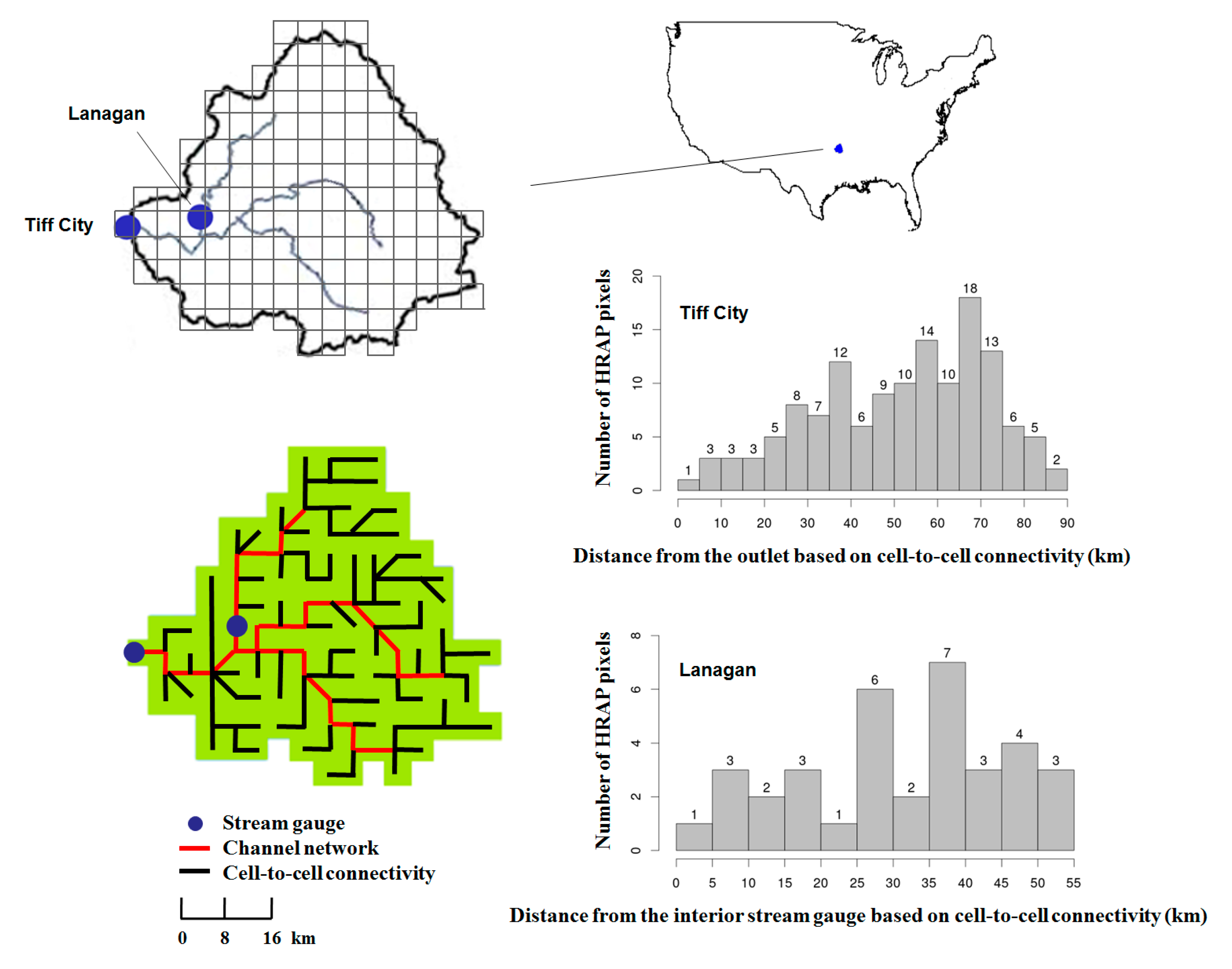
The study area used is the 2258 km² headwater basin that drains into the Elk River near Tiff City, Missouri. The runoff coefficient of this basin is 0.22 based on its annual precipitation of 1117 mm and runoff of 246 mm. The basin soil consists of 39.8% silty clay, 30.5% silty clay, and 25.8% silt loam, and the basin elevation varies from 229 to 457 m (Smith et al., 2004). In addition to the United States Geological Survey (USGS) stream gauge at the outlet (USGS ID: 7189000), an interior USGS gauge at Lanagan (USGS ID: 7188885) with the drainage area of 619 km² is used to assess the combined effect of correcting MFB in model states and assimilating interior flow observations on updated states and streamflow. Hourly streamflow observations are available for the period of October 1992 to July 2002 for Tiff City and May 2000 to May 2006 for Lanagan. Assimilation experiment was carried out for the period of May 2000 through May 2006 using model states from base model simulation for the period of October 1992 through April 2000. In total, 15 events with observed streamflow exceeding 200 m³/s were selected for the assimilation experiments described in Section 4. Figure 2 shows the study basin where Tiff City and Lanagan drain 135 and 35 HRAP cells, respectively. Histograms in Figure 2 show the number of HRAP cells with the same distance to stream gauges where the distance is computed based on the cell-to-cell connectivity information. As a study area of the DMIP project, further details on this basin are found at Smith et al. [39].

3.2. Evaluation Metrics

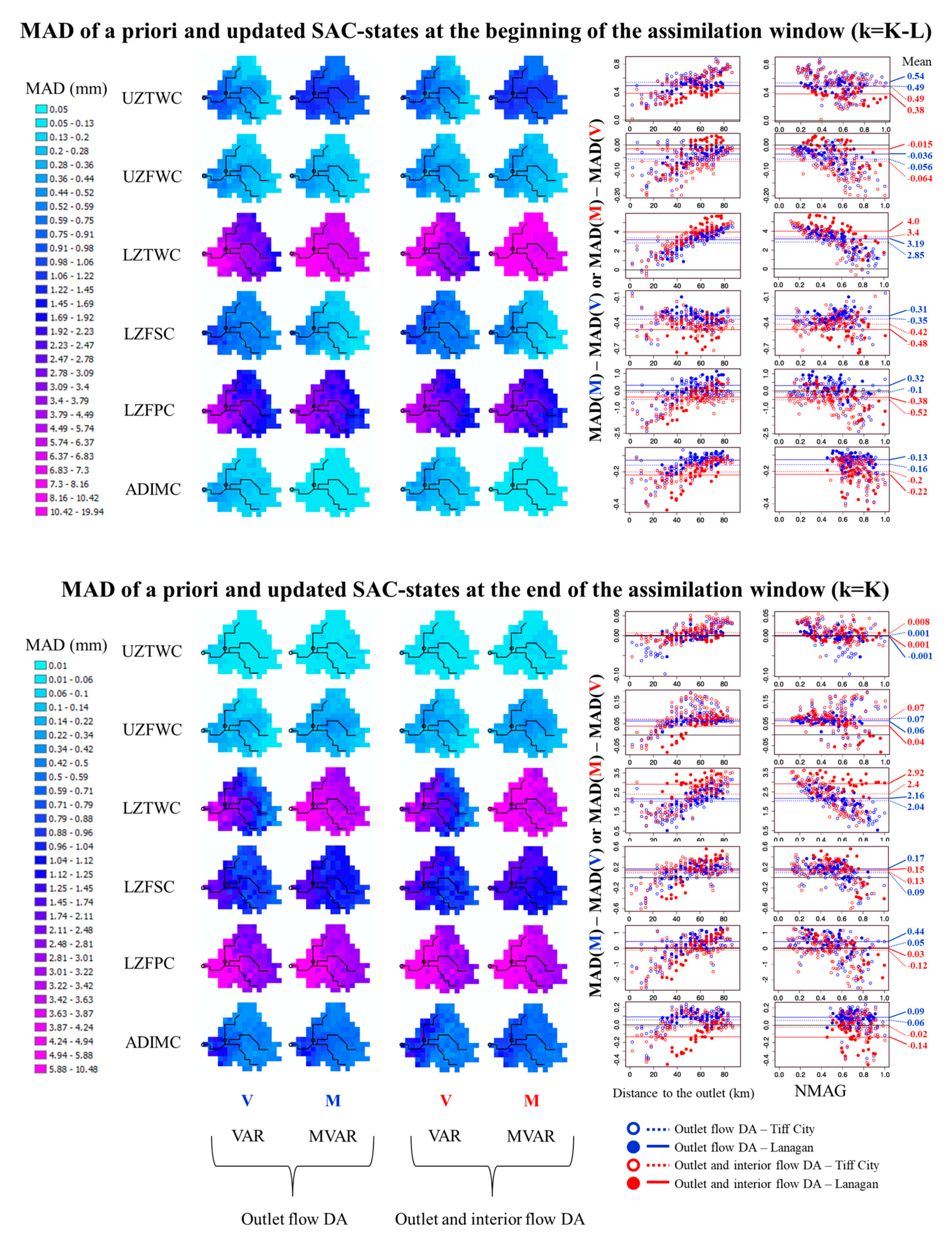
To quantify changes to model states posterior to the assimilation, the Mean Absolute Difference (MAD) between a priori and updated model states at time k is computed by Equation (17).

$$MAD=\frac{1}{N}{\displaystyle \sum }_{k=1}^N\left|X_{S,j,i}^{+}-X_{S,j,i}^{-}\right|$$

(17)

In Equation (17), $X_{S,j,i}^{-}$ and $X_{S,j,i}^{+}$ represent the a priori or updated, respectively, j-th state variable at the i-th grid. In the presence of MFB in model states, the MAD values from MVAR are expected to be larger than those from VAR at HRAP cells distant to stream gauges.

Mean Squared Error (MSE) of streamflow and its decomposition into bias, variance, and co-variance terms can be calculated with Equation (18).

$$MSE=\frac{1}{N}{\displaystyle \sum }_{k=1}^N{\left(Z_{Q,k}-H_{Q,k}\right)}^2={\left({\mu }_{Z_{Q,k}}-{\mu }_{H_{Q,k}}\right)}^2+{\left({\sigma }_{Z_{Q,k}}-{\sigma }_{H_{Q,k}}\right)}^2+2{\sigma }_{Z_{Q,k}}{\sigma }_{H_{Q,k}}\left(1-r\right)$$

(18)

where $r$ is the linear correlation coefficient between $Z_{Q,k}$ and $H_{Q,k}$; ${\mu }_{Z_{Q,k}}$ and ${\mu }_{H_{Q,k}}$ are means of $Z_{Q,k}$ and $H_{Q,k}$, respectively; ${\sigma }_{Z_{Q,k}}$ and ${\sigma }_{H_{Q,k}}$ are standard deviations of $Z_{Q,k}$ and $H_{Q,k}$, respectively. The three components of MSE in Equation (18) help identify the source of MSE change.

To evaluate the performance of MVAR and VAR at stratified flow ranges, Type-I and Type-II Conditional Biases (CB) can be computed by Equations (19) and (20).

$$\mathrm{Type}-\mathrm{I} \mathrm{CB}= Z_{Q,k}-E\left[Z_{Q,k}|H_{Q,k}\right]$$

(19)

$$\mathrm{Type}-\mathrm{II} \mathrm{CB}= H_{Q,k}-E\left[H_{Q,k}|Z_{Q,k}\right]$$

(20)

Type-I CB is conditioned on streamflow simulation $H_{Q,k}$ which tells falsely detecting non-existent events or the quality of the model calibration. On the other hand, Type-II CB is conditioned on streamflow observation $Z_{Q,k}$ which quantifies a failure of detecting existing events. Both CBs can be computed by slicing the scatter plots of $Z_{Q,k}$ on an x-axis and $H_{Q,k}$ on a y-axis horizontally for Type-I CB or vertically for Type-II CB into a number of intervals. Type-I and II CBs visualize performance changes from normal to extremes. Differences between Type-II CB and Type-I CB suggest the area of further enhancement.

4. Results

In this Section, an illustrative example of MVAR and VAR results from a single assimilation cycle is presented in Section 4.1, followed by the MAD of the two assimilation techniques in terms of model states or a soil moisture profile in Section 4.2. Section 4.3 describes the effect of weakly-constrained assimilation approaches in MVAR. Section 4.4 compares the performance of MVAR and VAR on streamflow.

4.1. Illustrative Example

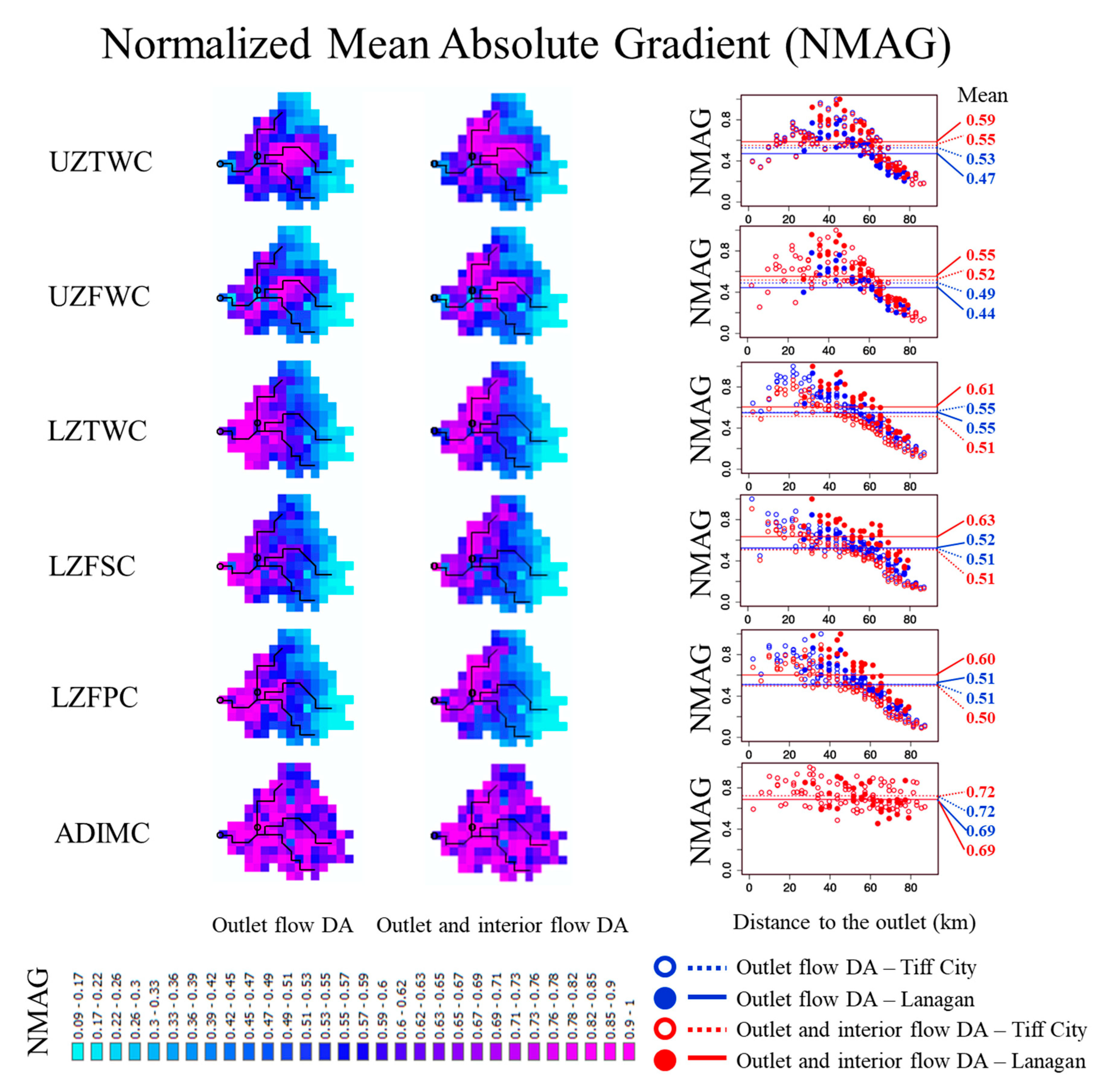
The sensitivity of the objective function ($J_K$) to background model states ($X_{S,j,i,K-L}$) at the beginning of the assimilation window, or $\frac{\partial J_K}{\partial X_{S,j,i,K-L}}$, tend to become lower with an increase of the distance to the stream gauges as shown in Figure 3 with the Normalized Mean Absolute Gradient (NMAG; Equation (21)) from all assimilation cycles.

$$NMAG=\frac{\left(\frac{1}{N}{{\displaystyle \sum }}_{k=1}^N\left|\frac{\partial J_K}{\partial X_{S,j,i,K-L}}\right|\right)}{\underset{i}{\max }\left(\frac{1}{N}{{\displaystyle \sum }}_{k=1}^N\left|\frac{\partial J_K}{\partial X_{S,j,i,K-L}}\right|\right)}$$

(21)

In Equation (21), $X_{S,j,i,K-L}$ denotes the j-th model state at the i-th HRAP grid at $k=K-L$.

In Figure 3, TWCs show higher sensitivity than FWCs. Despite the differences in the magnitude of gradients, all five soil moisture contents in UZ and LZ show a similar spatial pattern of NMAG, that is, NMAG decrease with an increase of the distance to stream gauges. Compared to UZ states, LZ states show slightly larger NMAG around the basin outlet, indicating a weak dynamic causality between outlet flow and deep soil moisture in distant cells. Compared to the case of outlet flow assimilation, additionally assimilating interior flow increases NMAG of UZ states at the scale of both a whole basin and the sub-basin Lanagan. However, the sensitivity of LZ states has reduced in terms of a basin mean, while the opposite is true in the case of Lanagan. ADIMC is overall little sensitive to the objective function at all HRAP cells.

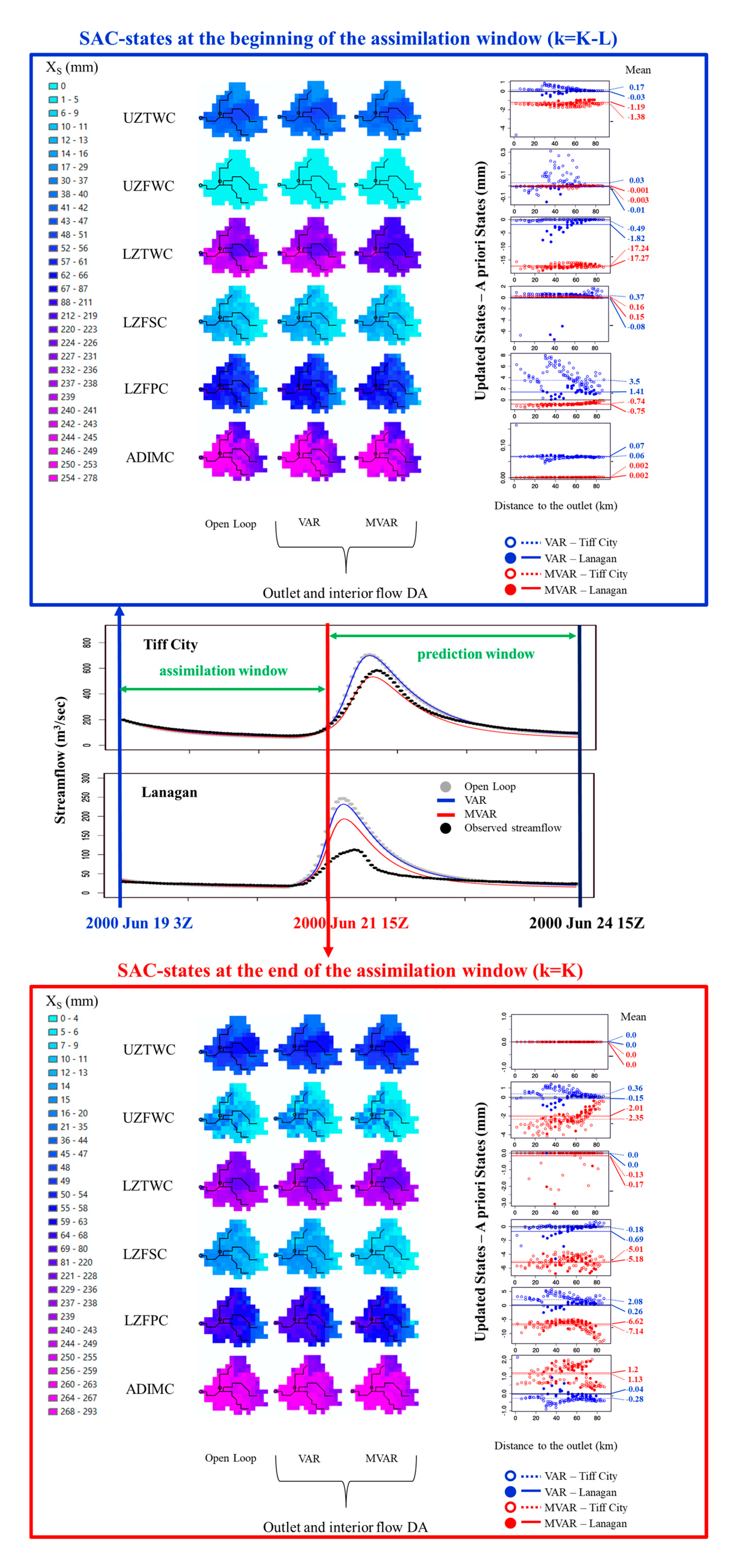
Figure 4 compares MVAR with VAR for a single assimilation cycle on June 21, 15Z, 2000. At the top panel of Figure 4, MVAR adjusts states spatially uniformly to address the flow volume error at the early rising limb of Lanagan as well as Tiff City as shown in the middle panel. On the contrary, the conventional distributed state updating suffers from improving streamflow (middle panel) by adjusting individual cell states (top panel), and the change in states is overall negligible at distant HRAP cells. The changed amount in SAC states from all assimilation cycles will be described in the following section. The bottom panel of Figure 4 presents the states at the time of forecast, which show how differences in TWCs at the beginning of the assimilation window ($k=K-L$) yields differences in FWCs at the end of the assimilation window ($k=K$) as initial conditions for prediction.

4.2. Model States

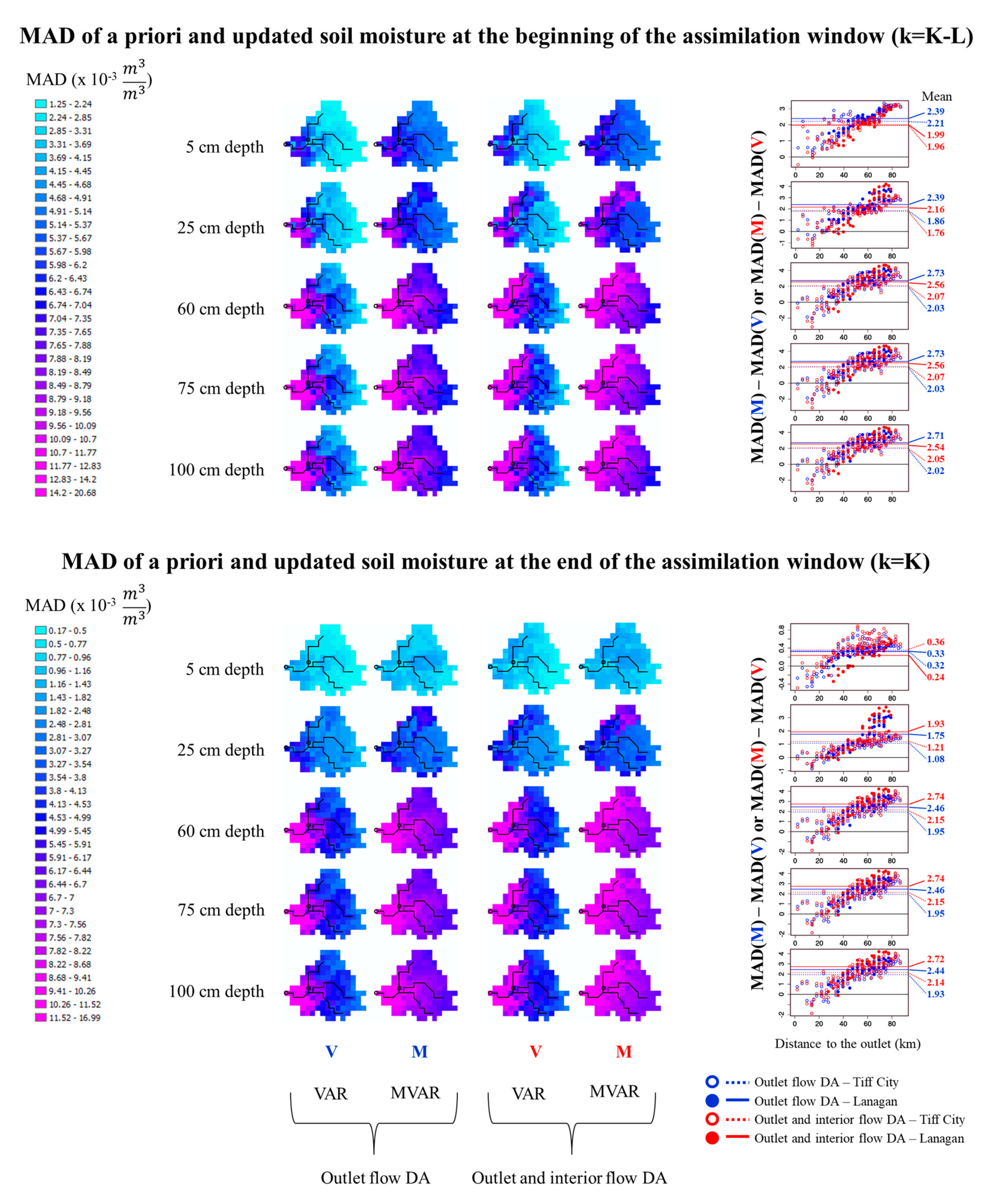
Through the MFB correction, MVAR is expected to update states at distant cells more largely than VAR for all model states except ADIMC with its small gradient values everywhere (Figure 3). This is shown in Figure 5 as an increasing pattern of MAD(M)—MAD(V) with an increase of the distance to the basin outlet where MAD (Equation (17)) quantifies the mean absolute difference of a priori and updated states; MAD(M) and MAD(V) represent MAD from MVAR or VAR, respectively; LZSFC at $k=K-L$ shows less of an increasing pattern than other soil moisture states possibly due to the objective function is less sensitive to LZSFC than the other states, as shown in Figure 3. In contrast, LZTWC with the largest sensitivity shows vividly an increasing pattern at both $k=K-L$ and $K$, compared to the rest states. In Figure 5, MAD differences tend to decrease with an increase of NMAG particularly in the case of LZTWC, which reflects the overall decreasing pattern of NMAG with an increase of the distance (Figure 3). When assimilating interior flows in addition to outlet flows, NMAG mean values of UZ and LZ tension and free water contents for Lanagan are always larger than those for Tiff City (Figure 3). This is shown in Figure 5 as MAD differences are larger for HRAP cells within Lanagan (solid red dots) than the rest (open red circles) in the case of assimilating interior flow in addition to outlet flow. This suggests a potential need of addressing biases at a sub-basin scale, that is, adjusting Local Bias (LB) instead of MFB—left for future work. In Figure 6, soil moisture at 5, 25, 60, 75, and 100 cm depths translated from SAC states shows consistently an increasing pattern of the MAD difference with an increase of the distance to the stream gauge at both $k=K-L$ and $K$—this supports the effectiveness of MVAR in updating soil moisture states at distant cells despite their little sensitivities to streamflow. Compared to a single scale DA used in Lee et al. [8], MVAR is able to noticeably update model states at distant cells (Figure 5 and Figure 6) while allowing updating model states at individual cells separately.

4.3. Model Structural Error

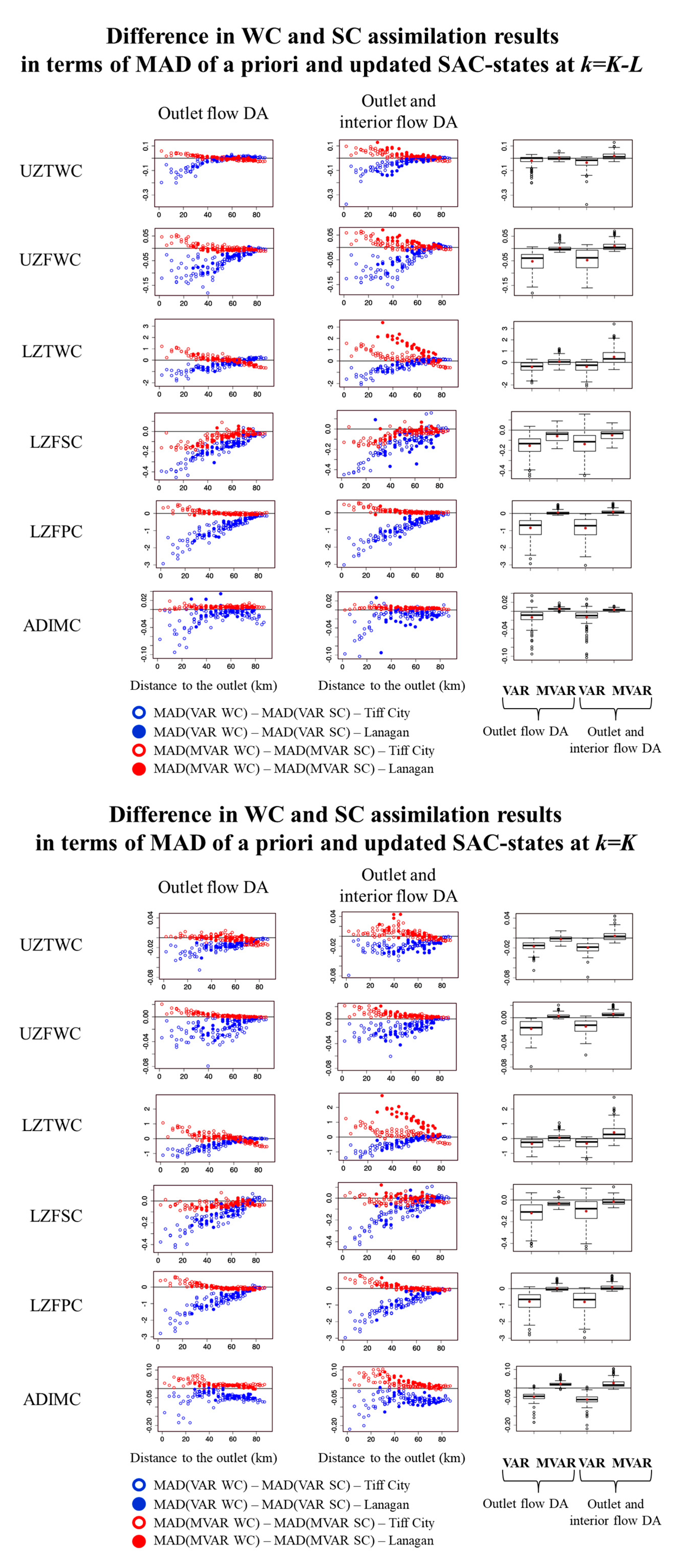
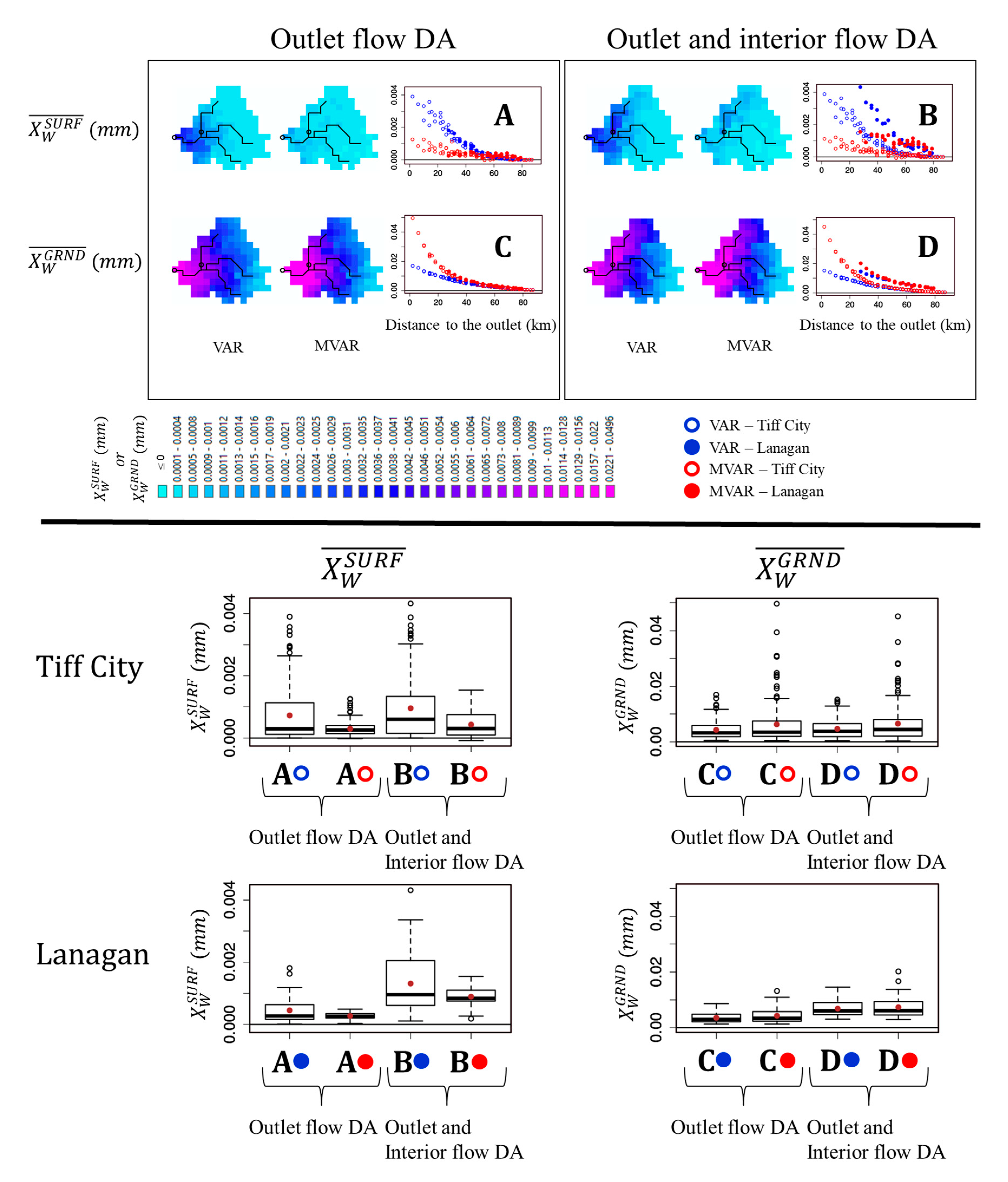
Differences between weakly- and strongly-constrained model results may reveal the reduced amount of model structural inadequacies owing to the MFB correction in MVAR when compared to corresponding VAR results. Figure 7 indicates that, except LZTWC, accounting for MFB in model states reduces the amount of additional adjustment for SAC-states by $X_W={\left[X_W^{SURF} X_W^{GRND}\right]}^T$. The distributed SAC-SMA model may be deficient in modeling deepwater evaporation from LZ (Koren et al., 2014), which in turn causes a larger estimation of $X_W^{GRND}$ in the case of MVAR than VAR (Figure 8), particularly at HRAP cells neighboring stream gauges. Equation (22) is used to compute $\overline{X_W^{SURF}}$ or $\overline{X_W^{GRND}}$ in Figure 8, which is the value averaged over the entire assimilation window (L) from all cycles (N − L + 1).

$$\overline{X_W}=\frac{1}{L\left(N-L+1\right)}{\displaystyle \sum }_{K=L}^N{\displaystyle \sum }_{k=K-L+1}^K{X}_{W,k,i}$$

(22)

The bottom panel of Figure 8 shows box plots of $\overline{X_W^{SURF}}$ and $\overline{X_W^{GRND}}$ at the scale of the entire basin Tiff City and the sub-basin Lanagan. At both Tiff City and Lanagan, MVAR produced notably smaller mean and value range of $\overline{X_W^{SURF}}$ ($A○B○A●B●$ in Figure 8) than VAR ($A○B○A●B●$) at both flow assimilation cases. In contrast, differences in $\overline{X_W^{GRND}}$ are marginal except outliers at Tiff City ($C○C○D○D○$ at the top right box plot in Figure 8). Figure 7 and Figure 8 suggest that, although MVAR generally reduces the effect of $X_W$ on model states by possibly reducing the degree of compensating for unresolved MFB by $X_W$, improving model fidelity to physical realism may precede an assimilation procedure in order to pose the assimilation problem well-posed [34]. When assimilating interior flows in addition to outlet flow, $\overline{X_W^{SURF}}$ and $\overline{X_W^{GRND}}$ values within Lanagan ($●$ and $●$ at the top panel of Figure 8) are conspicuously different from the rest ($○$ and $○$). This may indicate the changing amount of model structural errors as well as field biases resolvable via additionally assimilating interior flows which may benefit from adjusting LB at the scale of Lanagan, as discussed in Section 4.2.

Table 3. Time-averaged spatial correlation of background and updated model states. Values in the parenthesis represent correlation from VAR, or $r_V$, otherwise from MVAR, or $r_M$. Bold font highlights a larger value between $r_V$ and $r_M$. Underscored is the pair showing the minimum or maximum value of $r_M-r_V$ at either $k=K-L$ or $k=K$. WC and SC represent the model applied as a weak- or strong-constraint to the assimilation problem, respectively.

	UZTWC	UZFWC	LZTWC	LZSFC	LZPFC	ADIMC
	Begging of the assimilation window (k = K − L) Outlet flow assimilation
WC	0.995(0.991)	0.96(0.876)	0.88(0.883)	0.964(0.871)	0.981(0.96)	0.999(0.999)
SC	0.996(0.99)	0.969(0.853)	0.902(0.863)	0.966(0.854)	0.993(0.95)	0.999(0.999)
	Outlet and interior flow assimilation
WC	0.992(0.99)	0.952(0.859)	0.817(0.838)	0.956(0.828)	0.977(0.944)	0.999(0.998)
SC	0.994(0.989)	0.963(0.837)	0.854(0.817)	0.961(0.823)	0.99(0.935)	0.999(0.998)
	End of the assimilation window (k = K) Outlet flow assimilation
WC	0.999(0.999)	0.845(0.765)	0.913(0.97)	0.872(0.85)	0.947(0.932)	0.997(0.996)
SC	0.999(0.999)	0.842(0.752)	0.931(0.951)	0.883(0.841)	0.959(0.926)	0.997(0.995)
	Outlet and interior flow assimilation
WC	0.998(0.999)	0.821(0.754)	0.88(0.966)	0.814(0.768)	0.928(0.909)	0.996(0.994)
SC	0.999(0.999)	0.834(0.733)	0.912(0.945)	0.831(0.768)	0.943(0.901)	0.997(0.994)

shows the time-averaged spatial correlation of background and updated model states from both MVAR and VAR. In Table 3, MVAR generally retains higher spatial correlations than VAR at most states at all assimilation cases at both k = K − L and K. When the model is applied as a weak-constraint, MVAR-generated LZTWC shows consistently lower spatial correlations than the VAR-generated. As discussed above, this is also an indication of a need to improve model physics prior to the assimilation in order to preserve the spatial correlation structure of background model states as driven by base model simulation [34].

4.4. Streamflow

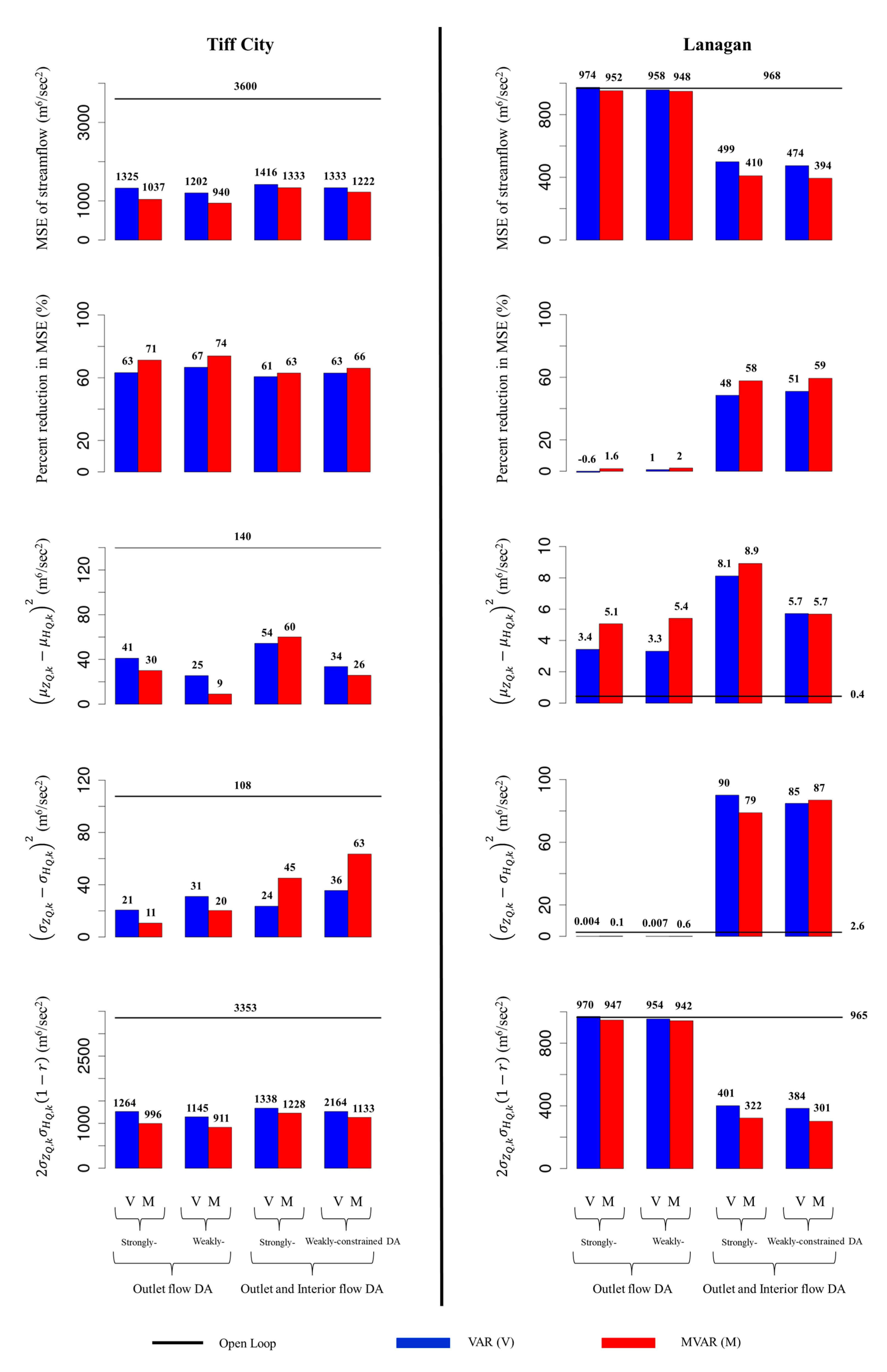
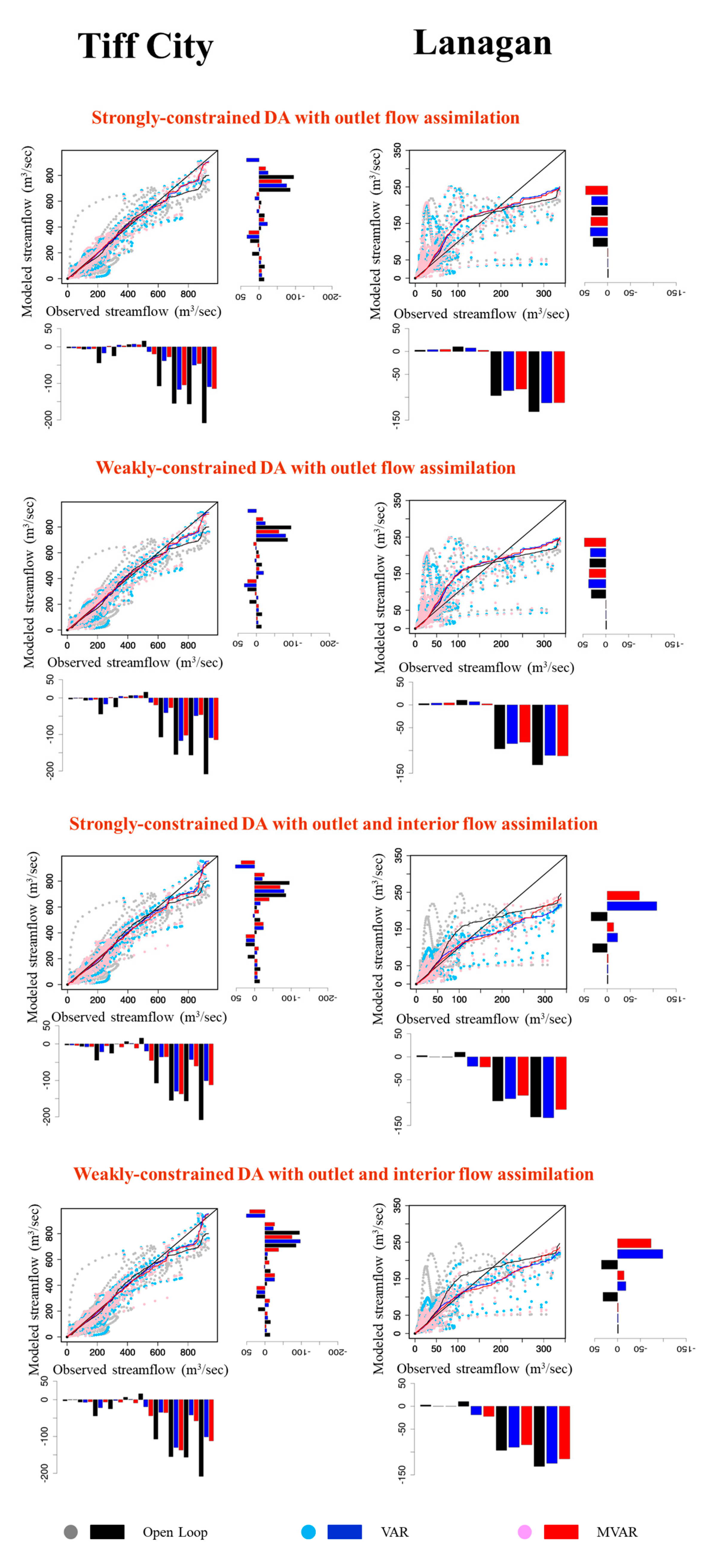
MVAR improved outlet as well as interior flow over the conventional VAR at all assimilation cases in terms of MSE (Figure 9). Compared to VAR, MVAR reduced further MSE of streamflow by 2–8% at Tiff City, and by 1–10% at Lanagan, depending on the data assimilated and the model applied as a weak- or strong-constraint to the assimilation problem (Figure 9). Assimilating interior flow in addition to outlet flow is necessary to achieve considerable improvement in interior flows by VAR [8], which is further improved by MVAR. Compared to strongly-constrained assimilation results, weakly-constrained assimilation reduced MSE of streamflow by 2–4% at Tiff City and by 0.4–3% at Lanagan. MSE decomposition into bias, variance, and co-variance indicates that MVAR outperforms VAR by better modeling co-variabilities of streamflow observation and simulation at both Tiff City and Lanagan at the cost of increasing bias and variance terms at some assimilation cases. In the case of assimilating outlet flow only, all three MSE components for outlet flow are consistently reduced by MVAR more than VAR, implying the positive effect of addressing MFB in model states on reducing bias and modeling variance as well as co-variance in simulated and observed flow. Magnitude-dependent performance is examined based on Type-I and –II CBs. In Figure 10, Type-I CB is generally smaller than Type-II CB particularly at extremes which signifies the importance of addressing Type-II CB in estimation and prediction of extremes [23]. In the case of assimilating interior flows in addition to outlet flow, median-range flows of less than 150 m³/s at Lanagan are mostly improved, whereas heavy-to-extreme flows at Lanagan are degraded (Figure 10). Visual examination of hydrographs at Lanagan indicated the notable amount of magnitude-dependent flow bias at some events which warrants future efforts with CB-penalized assimilation techniques such as CB-penalized Kalman Filter (CBPKF, [23]) or its ensemble extension, CB-penalized Ensemble Kalman Filter (CBEnKF, [9]).

5. Conclusions

The MFB-aware variational assimilation (MVAR) for the distributed SAC-SMA model was developed and comparatively evaluated with the conventional VAR based on its application to the headwater basin at Tiff City, Missouri. MVAR corrects MFB in model states and then update states at an individual HRAP grid. Compared to VAR [7,8,11,34], MVAR adjusts model states at remote cells by larger margins albeit their little sensitivities to streamflow. MVAR generally outperformed VAR in improving streamflow in both cases of outlet flow assimilation and interior as well as outlet flow assimilation. When the interior flow is assimilated in addition to outlet flow assimilation, improvement in interior flow is conspicuous. When the model is applied as a weak-constraint to the assimilation problem, MVAR generally less adjusted model states than VAR, implying the model error estimate possibly compensated for the MFB in model states in the case of VAR. The future work includes developing VAR with a capability to address spatially non-uniform biases in model states as well as magnitude-dependent biases in streamflow.

References

- Kitanidis, P.K.; Bras, R.L. Real time forecasting of river flows. R. M. Parsons laboratory for water resources and hydrodynamics. Tech. Rep. 1978, 235, 324. [Google Scholar]
- Sittner, W.T.; Krouse, K.M. Improvement of Hydrologic Simulation by Utilizing Observed Discharge as an Indirect Input (Computed Hydrograph Adjustment Technique—CHAT); NOAA Tech. Memo. NWS HYDRO-38: Silver Spring, MD, USA, 1979; p. 125.
- WMO. Simulated Real-Time Intercomparison of Hydrological Models. Operational Hydrology Rep. 38; World Meteorological Organization: Geneva, Switzerland, 1992; p. 241. [Google Scholar]
- Georgakakos, K.; Smith, G.F. On improved operational hydrologic forecasting: Results from a WMO real-time forecasting experiment. J. Hydrol. 1990, 114, 17–45. [Google Scholar] [CrossRef]
- Refsgaard, J.C. Validation and intercomparison of different updating procedures for real-time forecasting, Nord. Hydrol. Res. 1998, 28, 65–84. [Google Scholar] [CrossRef]
- Moradkhani, H.; Hsu, K.-L.; Gupta, H.; Sorooshian, S. Uncertainty assessment of hydrologic model states and parameters: Sequential data assimilation using the particle filter. Water Resour. Res. 2005, 41, W05012. [Google Scholar] [CrossRef] [Green Version]
- Lee, H.; Seo, D.-J.; Koren, V. Assimilation of streamflow and in-situ soil moisture data into operational distributed hydrologic models: Effects of uncertainties in the data and initial model soil moisture states. Adv. Water Resour. 2011, 34, 1597–1615. [Google Scholar] [CrossRef]
- Lee, H.; Seo, D.-J.; Liu, Y.; Koren, V.; McKee, P.; Corby, R. Variational assimilation of streamflow into operational distributed hydrologic models: Effect of spatiotemporal scale of adjustment. Hydrol. Earth Syst. Sci. 2012, 16, 2233–2251. [Google Scholar] [CrossRef] [Green Version]
- Lee, H.; Shen, H.; Noh, S.J.; Kim, S.; Seo, D.-J.; Zhang, Y. Improving flood forecasting using conditional bias-penalized ensemble Kalman filter. J. Hydrol. 2019, 575, 596–611. [Google Scholar] [CrossRef]
- Rakovec, O.; Weerts, A.H.; Hazenberg, P.; Torfs, P.J.J.F.; Uijlenhoet, R. State updating of a distributed hydrological model with Ensemble Kalman Filtering: Effects of updating frequency and observation network density on forecast accuracy. Hydrol. Earth Syst. Sci. 2012, 16, 3435–3449. [Google Scholar] [CrossRef] [Green Version]
- Lee, H.; Seo, D.-J. Assimilation of hydrologic and hydrometeorological data into distributed hydrologic model: Effect of adjusting mean field bias in radar-based precipitation estimates. J. Hydrol. 2014, 74, 196–211. [Google Scholar] [CrossRef]
- Nasab, A.R.; Seo, D.-J.; Lee, H.; Kim, S. Comparative evaluation of maximum likelihood ensemble filter and ensemble Kalman filter for real-time assimilation of streamflow data into operational hydrologic models. J. Hydrol. 2014, 519, 2663–2675. [Google Scholar]
- Dooge, J.C.I.; Napiôrkowsld, J.J. Applicability of diffusion analogy in flood routing. Acta Geophys. Pol. 1987, 35, 65–75. [Google Scholar]
- Jia, X.; Zeng, F.; Gu, Y. Semi-analytical solutions to one-dimensional advection–diffusion equations with variable diffusion coefficient and variable flow velocity. Appl. Math. Comput. 2013, 221, 268–281. [Google Scholar] [CrossRef]
- Nazari, B.; Seo, D.-J. Symbolic explicit solutions for 1-dimensional linear diffusive wave equation with lateral inflow and their applications. Water Resour. Res. 2020. [Google Scholar] [CrossRef]
- Li, Z.; Navon, I.M. Optimality of variational data assimilation and its relationship with the Kalman filter and smoother. Quart. J. Roy. Meteor. Soc. 2001, 127, 661–683. [Google Scholar] [CrossRef]
- Evensen, G. Sequential data assimilation with a nonlinear quasi-geostrophic model using Monte Carlo methods to forecast error statistics. J. Geophys. Res. 1994, 99, 10143–10162. [Google Scholar] [CrossRef]
- De Lannoy, G.J.M.; Reichle, R.H.; Houser, P.R.; Pauwels, V.R.N.; Verhoest, N.E.C. Correcting for forecast bias in soil moisture assimilation with the ensemble Kalman filter. Water Resour. Res. 2007, 43, W09410. [Google Scholar] [CrossRef] [Green Version]
- Reichle, R.H.; Koster, R.D. Bias reduction in short records of satellite soil moisture. Geophys. Res. Lett. 2004, 31, L19501. [Google Scholar] [CrossRef] [Green Version]
- Seo, D.-J.; Breidenbach, J.P. Real-time correction of spatially nonuniform bias in radar rainfall data using rain gauge measurements. J. Hydrometeor. 2002, 3, 93–111. [Google Scholar] [CrossRef] [Green Version]
- Wu, L.; Seo, D.-J.; Demargne, J.; Brown, J.D.; Cong, S.; Schaake, J. Generation of ensemble precipitation forecast from single-valued quantitative precipitation forecast for hydrologic ensemble prediction. J. Hydrol. 2011, 399, 281–298. [Google Scholar] [CrossRef]
- Seo, D.-J.; Herr, H.D.; Schaake, J.C. A statistical post-processor for accounting of hydrologic uncertainty in short-range ensemble streamflow prediction. Hydrol. Earth Syst. Sci. Discuss. 2006, 3, 1987–2035. [Google Scholar] [CrossRef] [Green Version]
- Seo, D.-J.; Saifuddin, M.M.; Lee, H. Conditional bias-penalized Kalman filter for improved estimation and prediction of extremes. Stoch. Environ. Res. Risk Assess. 2018, 32, 183–201. [Google Scholar] [CrossRef]
- Chepurin, G.A.; Carton, J.A.; Dee, D. Forecast model bias correction in ocean data assimilation. Mon. Wea. Rev. 2005, 133, 1328–1342. [Google Scholar] [CrossRef] [Green Version]
- Dee, D.P. Bias and data assimilation. Q. J. R. Meteorol. Soc. 2005, 131, 3323–3343. [Google Scholar] [CrossRef] [Green Version]
- Brown, J.D.; Wu, L.; He, M.; Regonda, S.; Lee, H.; Seo, D.-J. Verification of temperature, precipitation and streamflow forecasts from the NOAA/NWS Hydrologic Ensemble Forecast Service (HEFS): 1. Experimental design and forcing verification. J. Hydrol. 2014, 519, 2869–2889. [Google Scholar] [CrossRef]
- Brown, J.D.; He, M.; Regonda, S.; Wu, L.; Lee, H.; Seo, D.-J. Verification of temperature, precipitation and streamflow forecasts from the NOAA/NWS hydrologic ensemble forecast service (HEFS): 1. Streamflow verification. J. Hydrol. 2014, 519, 2847–2868. [Google Scholar] [CrossRef]
- Smith, J.A.; Krajewski, W.F. Estimation of the mean field bias of radar rainfall estimates. J. Appl. Meteorol. 1991, 30, 397–412. [Google Scholar] [CrossRef] [Green Version]
- Seo, D.-J.; Breidenbach, J.P.; Johnson, E.R. Real-time estimation of mean field bias in radar rainfall data. J. Hydrol. 1999, 223, 131–147. [Google Scholar] [CrossRef]
- Kim, T.-J.; Kwon, H.-H.; Lima, C. A Bayesian partial pooling approach to mean field bias correction of weather radar rainfall estimates: Application to Osungsan weather radar in South Korea. J. Hydrol. 2018, 565, 14–26. [Google Scholar] [CrossRef]
- Koren, V.; Reed, S.; Smith, M.; Zhang, Z.; Seo, D.-J. Hydrology laboratory research modeling system (HL-RMS) of the US national weather service. J. Hydrol. 2004, 291, 297–318. [Google Scholar] [CrossRef] [Green Version]
- Li, Z.; McWilliams, J.C.; Ide, K.; Farrara, J.D. A multiscale variational data assimilation scheme: Formulation and illustration. Mon. Wea. Rev. 2015, 143, 3804–3822. [Google Scholar] [CrossRef]
- Noh, S.J.; Weerts, A.H.; Rakovec, O.; Lee, H.; Seo, D.-J. Assimilation of streamflow observations. In Handbook of Hydrometeorological Ensemble Forecasting; Duan, Q., Pappenberger, F., Thielen, J., Wood, A., Cloke, H.L., Schaake, J.C., Eds.; Springer: Berlin/Heidelberg, Germany, 2018; pp. 1–36. [Google Scholar] [CrossRef]
- Lee, H.; Seo, D.-J.; Noh, S.J. A weakly-constrained data assimilation approach to address rainfall-runoff model structural inadequacy in streamflow prediction. J. Hydrol. 2016, 542, 373–391. [Google Scholar] [CrossRef] [Green Version]
- Burnash, R.J.; Ferral, R.L.; McGuire, R.A. A Generalized Streamflow Simulation System: Conceptual Modeling for Digital Computers; US Department of Commerce National Weather Service and State of California Department of Water Resources: Sacramento, CA, USA, 1973.
- Reed, S.M.; Maidment, D.R. Coordinate transformations for using NEXRAD data in GIS-based hydrologic modeling. J. Hydrol. Eng. 1999, 4, 174–183. [Google Scholar] [CrossRef]
- Reed, S.M. Deriving flow directions for coarse-resolution (1–4 km) gridded hydrologic modeling. Water Resour. Res. 2003, 39, 1238. [Google Scholar] [CrossRef]
- Natural Resources Conservation Service, United States Department of Agriculture, US General Soil Map (STATSGO2). Available online: https://data.nal.usda.gov/dataset/united-states-general-soil-map-statsgo2 (accessed on 10 December 2020).
- Smith, M.B.; Seo, D.-J.; Koren, V.I.; Reed, S.M.; Zhang, Z.; Duan, Q.; Moreda, F.; Cong, S. The distributed model intercomparison project (DMIP): Motivation and experiment design. J. Hydrol. 2004, 298, 4–26. [Google Scholar] [CrossRef]
- Koren, V.; Smith, M.; Cui, Z. Physically-based modifications to the sacramento soil moisture accounting model. Part A: Modeling the effects of frozen ground on the runoff generation process. J. Hydrol. 2014, 519, 3475–3491. [Google Scholar] [CrossRef]
- Sasaki, Y. Some basic formalisms in numerical variational analysis. Mon. Weather. Rev. 1970, 98, 875–883. [Google Scholar] [CrossRef] [Green Version]
- Zupanski, D. A general weak constraint applicable to operational 4DVAR data assimilation systems. Mon. Weather. Rev. 1997, 125, 2274–2292. [Google Scholar] [CrossRef]
- Di Lorenzo, E.; Moore, A.M.; Arango, H.G.; Cornuelle, B.D.; Miller, A.J.; Powell, B.; Chua, B.S.; Bennett, A.F. Weak and strong constraint data assimilation in the inverse regional ocean modeling system (ROMS): Development and application for a baroclinic coastal upwelling system. Ocean Model. 2007, 16, 160–187. [Google Scholar] [CrossRef]
- Moradkhani, H.; Sorooshian, S.; Gupta, H.V.; Houser, P.R. Dual state-parameter estimation of hydrological models using ensemble Kalman filter. Adv. Water Resour. 2005, 28, 135–147. [Google Scholar] [CrossRef] [Green Version]
- Ravela, S.; Emanuel, K.; McLaughlin, D. Data assimilation by field alignment. Phys. D Nonlinear Phenom. 2007, 230, 127–145. [Google Scholar] [CrossRef]
- Beven, K.J. On the concept of model structural error. Water Sci. Technol. 2005, 52, 167–175. [Google Scholar] [CrossRef] [PubMed]
- Seo, D.-J.; Koren, V.; Cajina, N. Real-time variational assimilation of hydrologic and hydrometeorological data into operational hydrologic forecasting. J. Hydrometeorol. 2003, 4, 627–641. [Google Scholar] [CrossRef]
Figure 1.
A schematic of the Mean Field Bias (MFB)-aware VAR (MVAR) which corrects MFB in model states via streamflow assimilation.
Figure 2.
The TIFM7 study basin (2258 km2); Lanagan (619 km2) stream gauge is about 28 km from the basin outlet calculated based on the cell-to-cell connectivity. The sub-basin Lanagan consists of 35 HRAP cells (~26% drainage area of the basin).
Figure 3.
Time-averaged, normalized absolute gradient values of the objective function (Equation (15)) with respect to individual model states, or NMAG in Equation (21), evaluated at each HRAP cell. The largest gradient value for UZTWC, UZFWC, LZTWC, LZSFC, LZPFC, and ADIMC are 85 (86), 11 (11), 261 (301), 9 (10), 52 (58) and 0.00005 (0.00005) (mm−1) in the case of assimilating outlet flow (outlet and interior flow).
Figure 4.
An example of comparing MVAR and conventional VAR results for a single assimilation cycle issued on June 21, 15Z, 2000. The sizes of assimilation and prediction windows used were 60 and 72 h. The model is applied as a strong-constraint to the assimilation problem and data assimilated includes outlet as well as interior flow observations. MFB estimates, or in Equation (1), are 0.9662, 1.0002, 0.9269, 1.0162, 0.9865, and 1.0 for UZTWC, UZFWC, LZTWC, LZSFC, LZPFC, and ADIMC, respectively.
Figure 5.
Mean absolute difference (MAD) of a priori and updated SAC-states at the begging (k = K − L; top panel) or end (k = K; bottom panel) of the assimilation window where the model is applied as a strong-constraint to the assimilation problem.
Figure 6.
Same as Figure 5 but for depth-specific soil moisture translated from SAC-states via the soil moisture translation routine available in the SAC-HT.
Figure 7.
Differences in weakly- (WC) and strongly-constrained (SC) assimilation results in terms of MAD of background and updated model states at the beginning (k = K − L; top panel) or end (k = K; bottom panel) of the assimilation window. Box plots were created using the entire basin results, that is, Tiff City.
Figure 8.
and (Equation (22)) from MVAR and VAR.
Figure 9.
Mean Squared Error (MSE) of streamflow analysis generated from VAR (V) or MVAR (M) and its decomposition (Equation (18)) where and are 125 (m3/s) and 157 (m3/s) for Tiff City, and 30 (m3/s) and 43 (m3/s) for Lanagan.
Figure 10.
Scatter plots of observed and simulated flow from the open loop, VAR, and MVAR at Tiff City and Lanagan. Type-I (Equation (19)) and Type–II (Equation (20)) conditional biases in streamflow are shown as bar plots on the right-hand side or at the bottom, respectively, of the scatter plot.