
Dynamic Pricing Recognition on E-Commerce Platforms with VAR Processes


1
Alten Italia, 35131 Padua, Italy
2
Department of Statistical Sciences, University of Padua, 35121 Padua, Italy
*
Author to whom correspondence should be addressed.
Forecasting 2021, 3(1), 166-180; https://0-doi-org.brum.beds.ac.uk/10.3390/forecast3010011
Submission received: 21 December 2020
/
Revised: 23 February 2021
/
Accepted: 1 March 2021
/
Published: 5 March 2021
(This article belongs to the Special Issue New Frontiers in Forecasting the Business Cycle and Financial Markets)
Abstract
:In an environment such as e-commerce, characterized by the presence of numerous agents, competition based on product characteristics is a very important aspect. This paper proposes a model based on vector autoregressive processes (VAR) and Lasso penalization to detect and examine the dynamics that govern real-time price competition in electronic marketplaces. Employing this model, an empirical study was performed on the price trends of smartphone models on the major electronic sales platforms of the Italian market. The proposed model detects real-time price variations in single vendors, based on the variations of their direct competitors. The statistical method adopted in this analysis may be useful for e-commerce companies that conduct market analyses of competitors’ pricing strategies.
JEL Classification:
C01; C5; C321. Introduction
In recent years, the volume of sales on e-commerce platforms has grown considerably. Today, it is not uncommon to find many offers with different prices for the same product at the same time. Thus, online real-time pricing has assumed a role of fundamental strategic importance. On one hand, companies have to constantly adjust their price levels based on competitors’ prices for the same products to appeal to customers, without losing revenue margins. On the other hand, customers are given the possibility of accessing all available prices for a given product with just a few clicks. The targets of this technique are companies interested in studying a market for strategic advantage over competitors in pricing policies and online shoppers who could benefit greatly from a service, which, based on real-time data, detects whether the price of a certain product is likely to increase/decrease in the short term. Retail is defined as the transaction of goods or services from the producer, or a sales intermediary, to the final consumer. It may occur through many channels, which can be grouped into two categories: The first reflects the traditional business model, called “bricks and mortar”, and is characterized by physical shops and stores where consumers go to make their purchases. The second, formed more recently, is carried out through the Internet, as a means of connecting supply and demand. The latter is known as e-commerce, and consists of the exchange of goods and services through the use of telecommunications and information technology, falling within the more general field of e-business.
This paper focuses on pricing strategies on e-commerce platforms in the presence of competition. E-commerce companies face new and challenging pricing policies for their products, as competition for any product is much fiercer. Consumers can access information on any product online and compare products across multiple platforms with just a few clicks. The market of interest is the sale of smartphones through e-commerce platforms in Italy. Specifically, this study analyzed three smartphone models, namely, “iPhone X,” “Galaxy S10” and “P30”, produced by Apple, Samsung and Huawei, respectively. At the time of data collection, these smartphones represented the latest models from the biggest phone manufacturers in terms of revenue and reputation worldwide. The selected models belong to the same value range within each brand. For example, in the case of Apple, its latest models (at the time of writing) consisted of three models: the iPhone XR (least expensive), iPhone X (intermediate) and iPhone XS (most expensive). This guaranteed that the dynamics underlying the purchasing processes for the three smartphones were relatively comparable. Smartphones, which include those considered in this analysis, may be classified as primary consumer goods, satisfying the primary need of communication. At the same time, smartphones take on some of the characteristics of luxury goods, i.e., goods that do not necessarily satisfy basic needs and for which the amount of money paid is not proportional to the real value of the product itself. Whenever a new smartphone is released, it is not uncommon to witness long queues of customers eager to get their hands on the latest model.
Prices are lowered over time due to the intrinsic technologic obsolescence of smartphones and the gradual loss of value due to the release of newer, more advanced models. The sector is also characterized by multiple resellers that offer the same product to end consumers, resulting in many companies adopting dynamic pricing strategies.
This paper examined the dynamics of direct price competition on smartphone sales in electronic marketplaces, by employing vector autoregressive (VAR) processes. These processes allow study of the interdependence between various time series of prices of the same products and possibly the prediction of future price variations. However, given the large number of e-commerce vendors for numerous products, the output of these models proved hard to read and interpret. Therefore, the model was applied by accounting for a Lasso penalization to detect interdependent price variations more efficiently. The main goal of this analysis was the real-time price variation detection of a specific smartphone model sold by a specific retailer based on its previous price changes and, more importantly, on the price variations performed by competitors selling the same model. Through an empirical study carried out over two months, the proposed model allowed us to efficiently and clearly identify direct price competition in terms of dynamic pricing during the observation period. With this analysis, the paper aims to contribute to the literature on using VAR models for marketing problems, by focusing on the context of e-commerce, with a newly created dataset through a web-scraping procedure.
The paper is structured as follows. Section 2 proposes a review of the background literature concerning the use of VAR models in the marketing and retail context. Section 3 discusses some concepts of marketing mix on e-commerce platforms, focusing on price competition. Section 4 illustrates the statistical methodology employed for the analysis. Section 5 presents the process of data collection and model estimation and interpretation. Section 6 discusses the main findings of the analysis, while Section 7 proposes concluding remarks and a discussion of the study limitations.
2. Background
Commercial markets have become increasingly complex environments, where multiple agents act and interact with each other in different ways, either collaborating or competing. On one hand, firms and retailers seek to gain market share and realize profit maximization by constantly proposing new products, applying price discounts and promotions, adding services and features to their offer to retain customers, gain new ones, improve the level of satisfaction and therefore, differ from competitors. On the other hand, consumers today are more mature and informed agents. They share knowledge and information regarding products and services and can access and compare a wide variety of substitute products in physical stores or on the Internet, thus becoming more selective in their final choice. In particular, the growing importance of e-commerce has emphasized these phenomena by making markets even more dynamic and competitive settings. In a recent review of theory and practice of forecasting, in a section specifically devoted to e-commerce, [1] emphasized that online retail modeling and forecasting must be especially agile and responsive to the latest decisions in the market, and integrated into the retailer’s strategies.
As many marketing data come in the form of time series, such as a product’s sales or price dynamics, time-series models have always played a central role. The authors of [2], discussed the central role of competition in marketing and proposed vector autoregressive moving average models (VARMA) as a useful tool for the purpose. In a review of statistical models in marketing, [3] focused on the role of VAR models for approaching time-series data in marketing, thanks to their ability to account for interdependencies among different time-series. The authors of [4], in a review on time-series models in marketing, suggested that VAR models may efficiently exploit the advantages of longer time-series and provide a important tool for understanding the evolving behavior of a market. The authors also identified some future challenges of markets that have become a reality, including the availability of larger datasets with a large number of variables, high-frequency data from the Internet and fast-changing and turbulent markets, where competitive reaction is a very important area. The authors of [4] observed, for example, that when Amazon announced a substantial discount on its best-seller books, Barnes and Noble matched the discount within hours.
Similar fast reactions to competitors’ choices are routine today, yet it is crucial to recognize those that have a significant impact.
In this sense, if VAR models have been identified as suitable tools for modeling possible interactions among time series, many authors have observed that the number of parameters in these models explodes rapidly, undermining the possibility of identifying important relationships. Among others, this issue was addressed by [5], who proposed a subset selection procedure for VAR models based on the Lasso penalization introduced by [6], and more recently, by [7], who developed an interesting extension of this approach based on the group Lasso model, which is able to guarantee some forecasting improvements over simpler methods, yet maintaining interpretability. In the marketing and retail literature, there are some relevant contributions employing VAR models with Lasso penalization, such as the study performed by [8], aimed at identifying significant within- and cross-category effects in a product category network, finding that categories have asymmetric roles in the network. Another important contribution, dealing with the problem of high dimensionality in retail, was provided by [9], focusing on the case of SKU retail sales forecasting with intra- and inter- category promotional information. In this paper, the authors developed a four-step framework to overcome the problem of high dimensionality, using a multistage Lasso regression. The issue of how to deal with high dimensions was discussed in [10]’s recent review of retail forecasting.
3. Marketing Mix in E-Commerce Platforms
The concept of marketing was defined in [11] as the process of exploring, creating and distributing value in order to satisfy specific needs of consumers in a specific market while making a profit. Through marketing, all decisions and strategies adopted by a given company in achieving its objectives are defined.
In the original formulation by [12], marketing is governed by four fundamental levers, called the 4Ps: product, price, place and promotion. Product refers to the goods or services being sold. The variable price represents the monetary counterpart the consumer is willing to pay for a given product. It is determined by the company through specific policies called pricing. Place is the set of activities and structures or buildings necessary to bring a given product to the final consumer (e.g., stores and shops). Promotion refers to all communication activities between the company and the consumer in general, for example, customer care or advertising. The set of decisions concerning the 4Ps is also called a company’s marketing mix.
Applying this framework to an online context where multiple vendors are present for the same category of product, the marketing mix variables involved are reduced to three: price, place and promotion. There is no longer any competition in product characteristics, which are common to all competitors in the market. The variables of promotion and place are closely linked, and sometimes the boundary between the two is not clearly definable. Basically, one can consider the joint effect of place and promotion by interacting with the graphical interface of the website on which the product is sold. The e-platform not only replaces the traditional physical store where customers go to purchase products but also provides fundamental assistance to customers, such as effective management of returns, acceptance of complaints and general customer care throughout the customer purchase experience.
With regard to price competition, there are various digital platforms specifically developed to allow consumers to compare prices of products online, such as Google Shopping. The very fact that multiple companies offer this service shows that although place and promotion have the same levels and characteristics, price plays a fundamental role in e-shoppers’ purchase decision process. In this way, e-commerce companies have to deal very carefully with the pricing policies of their products, as even the slightest deviation from the competition can result in lost revenue or possible gains. Of course, the common goal of all companies is profit maximization. Given the high competitiveness in products that characterizes e-commerce, this maximization comes with a trade-off between sales profitability and market competitiveness. Although companies tend to seek the maximization of mark-up (i.e., profit, calculated as the difference between the price of a product and its cost of production), they cannot ignore that, for the same product, the price is inversely proportional to its competitiveness in the market. For example, a price that is too high would lead consumers to prefer the competitor’s products. To adopt the highest possible price for products, companies resort to various pricing strategies. The first strategy, called price skimming, aims to make customers more willing to spend on a given good or service. In this way, as much of the consumer’s possible revenue is absorbed as possible. In practice, this strategy initially consists of setting the highest possible price, sometimes referred to as the launch price, and then gradually reducing the price to appeal to customers willing to pay less.
The second strategy that e-commerce companies adopt is what is known as competitive pricing. This pricing strategy is most common for companies in the same sector and is an important characteristic for markets with free competition. If, for example, for the same product, one company’s price is higher than the prices of all its competitors, the probability of making many sales will be very low, if at all.
The third strategy, similar but in some ways the opposite of competitive pricing, is dynamic pricing. This strategy does not consist, as with competitive pricing, of simply taking competitors’ prices into account, when setting one’s own price, but of setting a price that is exclusively based on competitors’ price levels. Sometimes, companies decide to monitor their competitors’ prices in real-time, through specifically developed algorithms that process competitors’ prices or consumers’ data, and adjust their prices accordingly. In situations where a dynamic pricing strategy is adopted, in the event that a company raises its price, its competitors have several options for action. The first is to adjust price levels with a consequent price increase, given the decrease in the general price competition in the market. Another possibility is to keep the price constant and benefit from customers do not prefer the competitors, by adopting a strategy called shadow pricing.
4. Methodology
The approach adopted in this paper is based on the VAR model [13]. This model allows to examine the values of a time series at a given time as a function of its own past values, but also to taking into consideration the interaction between different interdependent time series.
The VAR model is typically specified as
where is a vector of k endogenous variables and are the matrices of the parameters of the VAR process with p lags of previous observations that have been taken into account. For further details, refer to [14,15].
However, a significant obstacle to the use of VAR models is when the number of considered time series k is large. The total number of parameters of the unconstrained model equals , where k is the number of time-series and p is the lag order [5]. To solve this issue, the Lasso penalty introduced by [6], may be applied in the model estimation process, to reduce the number of parameters to be estimated [5]. The coefficients, therefore, are reduced, with a penalty applied to the objective function; in the VAR model case, the minimum least squares. In this way, in addition to the reduction in the parameters, parameters that have values below a certain threshold are forced to zero. This allows the performance of parameter selection and identification of the strongest interdependencies between variations in different time series. Loss function that characterizes the estimation of the parameters of the final model is
where , also called the companion matrix, contains the matrices with the VAR parameters, considering up to p lags and the tuning parameter the Lasso penalization performed on the parameters. (The Lasso regularization is employed by applying the cross-validation method equation by equation, separately). When is small, the result is essentially the least-squares estimates; while as increases, shrinkage occurs, so that some parameters are set equal to zero [16].
One metric for evaluation for goodness of fit is the mean squared forecast error (MSFE), i.e., the average quadratic forecast error. This metric is calculated after dividing the dataset into three parts in chronological order , (where is the latest time instance of a specific iteration). For each iteration, the first part is used for parameter initialization, the second for penalty parameter selection and the last observation T for the test set. The final value of adopted is the one for which the MSFE is minimized, i.e., using the method known as rolling cross-validation [7]
where and are the value of the forecast calculated with a certain value of and the true value, respectively. With the rolling cross-validation technique, instead of using as test sets’ randomly extracted data, the training sets consist only of observations that occurred before the last observation, which form the test sets. In this way, only past observations are used in the evaluation of the MSFE of the last available test set. In other words, there are as many test sets, each consisting of a single observation, as there are observations in the training set . Rolling cross-validation differs from the usual k-fold cross-validation [16], since the time dependency is taken into account.
5. Dynamic Pricing Recognition in Smartphone Sales
5.1. Data Retrieval
The modeling approach presented in Section 4 was applied to a dataset concerning the prices, expressed in euros, of the latest smartphones from Apple, Samsung and Huawei, sold on e-commerce platforms. Data were collected twice a day, around 8 a.m. and around 6 p.m., respectively, at the beginning and at the end of a hypothetical work day. The observations cover a period of two months, from August to October 2019, summing up to 120 entries. In this way, it was hypothesized that potential price variations were captured up to a daily granularity and consequently reported in the final dataset.
At the operational level, through the use of specifically developed scripts in Python, online data-scraping was performed on e-commerce platforms, such as Google Shopping. The final dataframe was made of rows (observations) and columns (vendors). However, before model estimation, it was necessary to carry out some pre-processing operations.
5.2. Pre-Processing
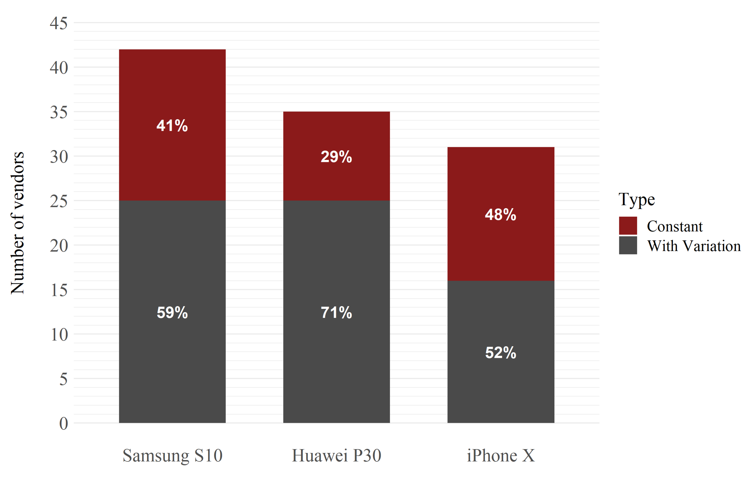
As the main interest was the study of price variations and their influence on competitors, an important data-cleaning operation was the removal of time series that did not show any variations throughout the observation period. Therefore, all constant time series were excluded from the dataset. A total of 42 vendors were removed. This is interesting, because 39% of the total retailers did not make any changes to the prices of their products during the study period. In particular, as shown in Figure 1, the percentage of time series without variation is higher for the iPhone X, compared to those for the other two smartphones.
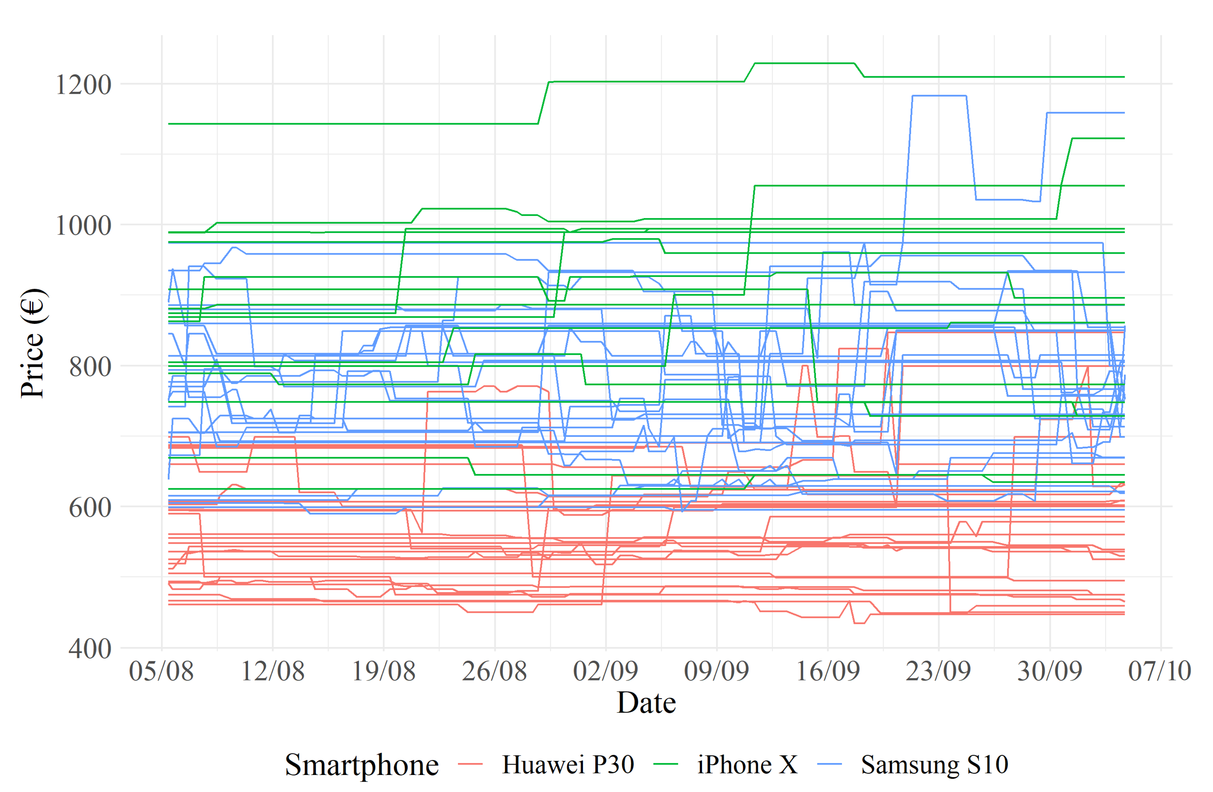
Another fundamental issue to address was related to missing data imputation in the dataset. Out of a total of 7986 observations, 40% (3242) of the datapoints were missing. In the context of this study, there was no evidence of a systematic process underlying the missing data, and therefore, it was assumed that a missing data value corresponded to a lack of price variation. From a practical point of view, this assumption led to the following rule: If a price could not be scraped at a given time moment t, its value was equal to the immediately previous available observation of the same reseller. This technique is known as last observation carried forward (LOCF) [17]. The data extracted after the missing value imputation are displayed in Figure 2.
To use the VAR model, each time series needed to satisfy the stationarity condition. However, none of the price time series were strongly non-stationary, according to the augmented Dickey–Fuller test (ADF) [18]. Through the application of a first difference to each available time series, stationarity was obtained. The ADF tests, calculated for each time series up to the lag led to rejection of the null hypothesis of non-stationarity in favor of the alternative hypothesis of stationarity with a p-value for each time series present in the dataset. Consequently, the final data type used in the analyses was the price variation relative to the previous price of each vendor. This implied that the object of analysis was not the specific price level, but the price variation at time t versus time for each vendor.
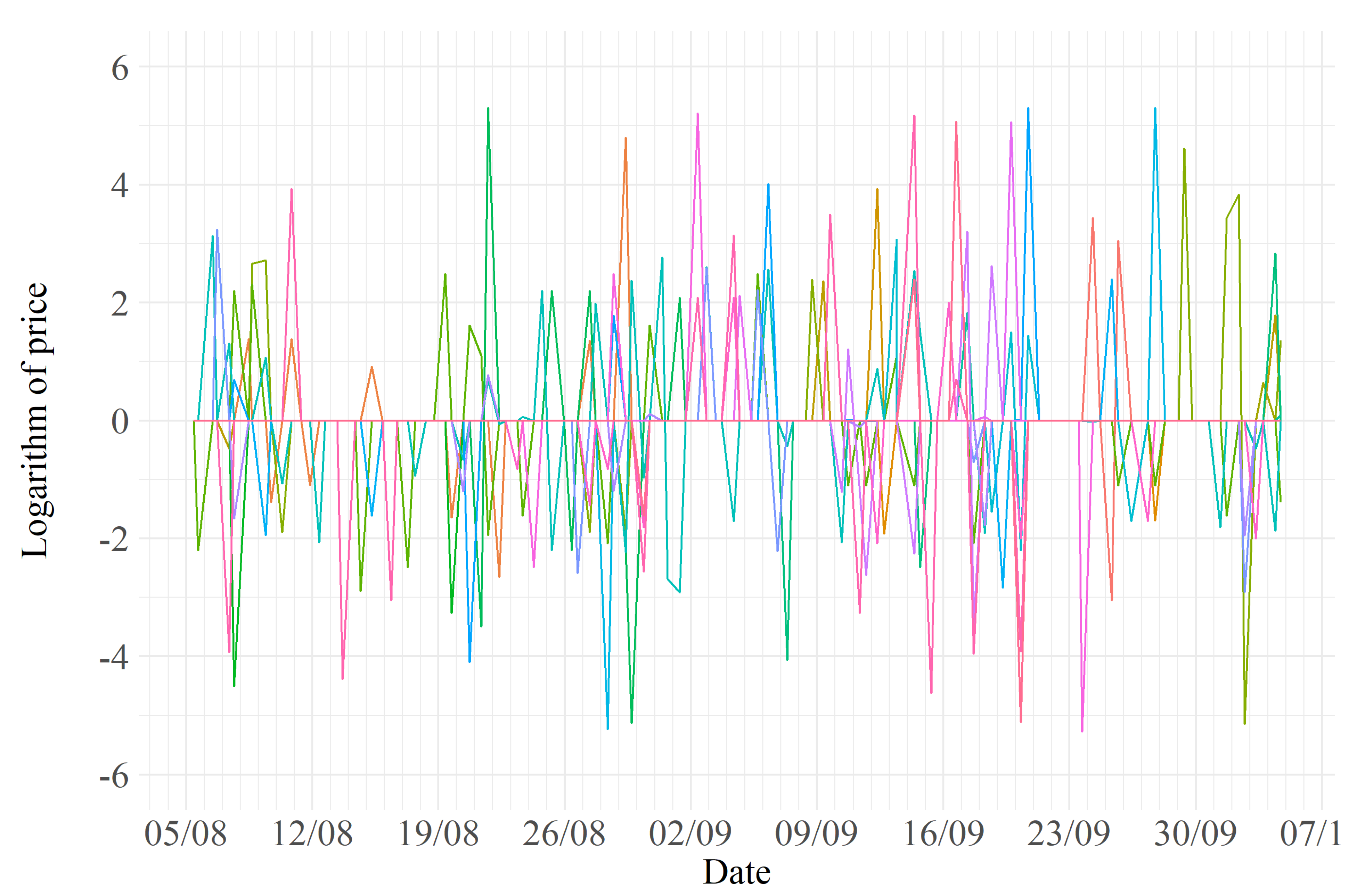
Moreover, as the observed data were characterized by low and high price variations, from a few cents up to about 250 EUR, it was found reasonable to apply a further transformation to the data, namely, a logarithmic transformation of the price changes, in order to re-scale larger values. As negative values and values equal to zero were present, the following variant of the logarithmic transformation, allowing to keep the directionality (positive or negative) of the price variation, was applied: .
This specific data transformation was adopted to uncover those vendors that systematically employed dynamic pricing strategies, being the main focus of the analysis.
An attempt to estimate a VAR model after applying only the first difference was carried out. A total of 17 non-zero parameters were returned. After inspection of those vendors associated to the non-zero parameters, it was clear that the model estimated on the first difference of the prices returned those pairs of vendors which had one or two interactions of big price changes close in time, while the majority of vendors did not seem to systematically change their prices to answer a competitor’s price change. In order to contrast this aspect of the estimated VAR model, we decided to apply the log transformation, in order to rescale the price changes, by penalizing high values. This allowed the model to account also for smaller price changes and to identify those vendors that presented dynamic pricing strategies more frequently. Another attempt to use the difference of logs of the observed prices was also carried out. In this case, however, as in the case where the price time series were only first differentiated (without log transformation), only 15 non-zero parameters were returned. All pairs of vendors associated to these 15 parameters presented the same characteristic of having big one-time interactions, rather than many price adjustments, that is dynamic pricing.
5.3. Descriptive Analysis
The first visual analysis of the time series before transformation in Figure 2 shows that the three smartphones, grouped by color, had different average price levels. Table 1 shows the number of vendors and the minimum, average, maximum and standard deviation values for the transformed data, grouped by smartphone. The minimum, maximum and average values were almost equivalent for all the smartphones. The standard deviation was highest for the Samsung S10, followed by the Huawei P30. The standard deviation and the number of vendors for each smartphone were inversely proportional to the average price of the corresponding smartphones. A reasonable explanation for this phenomenon could be that price competition is greater, resulting in more price changes for less expensive products, as they are purchased by consumers who are price-sensitive.
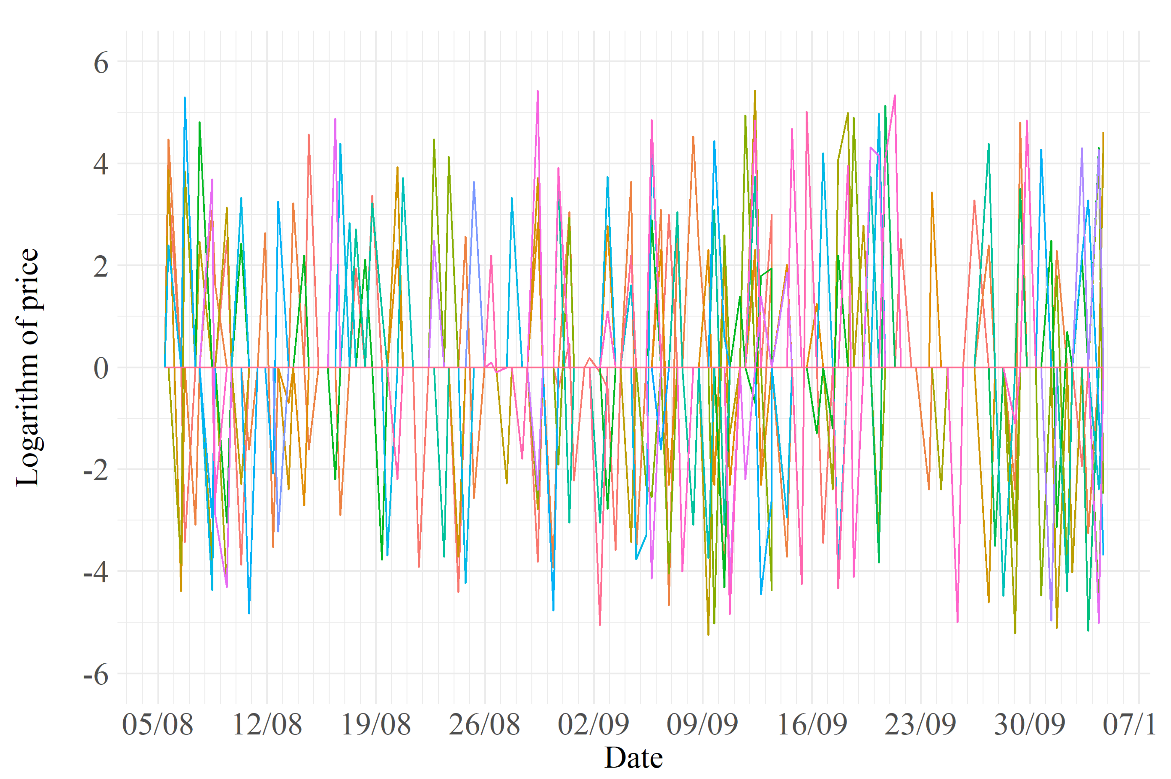
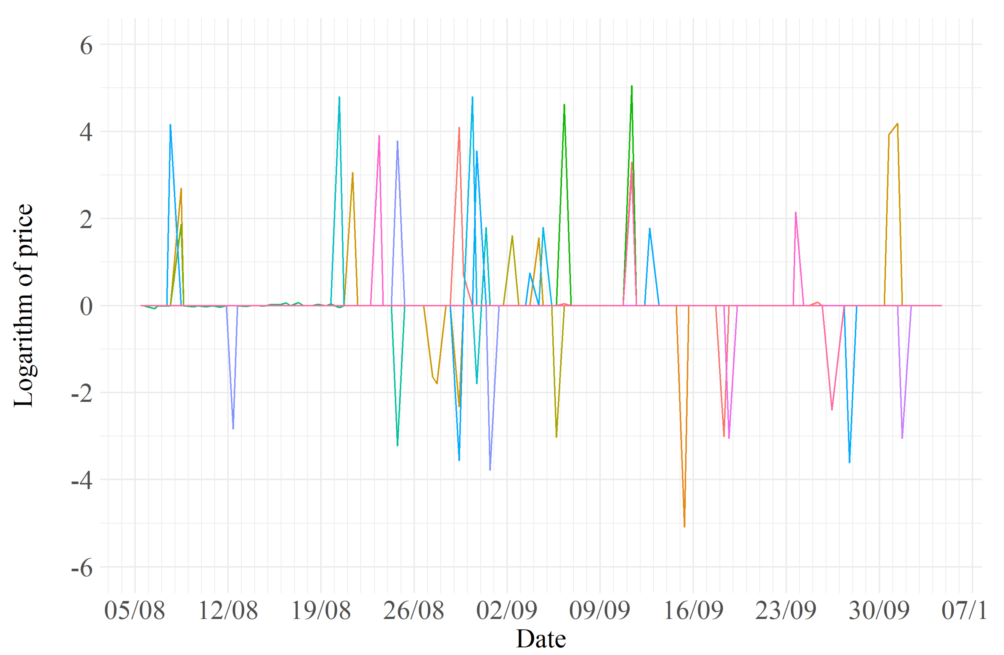
Figure 3, Figure 4 and Figure 5 show the transformed price variation data that make up the final dataset. A first inspection of these figures may suggest some preliminary observations: it is evident that the market for the Samsung 10 has more competitors and, therefore, dynamic pricing is more likely to take place. On the other hand, a less competitive environment seems to characterize the iPhone X.
5.4. Model Estimation
A fundamental aspect of VAR models concerns the choice of the p parameter. In this case, this parameter was not only based on a forecast error criterion, as is, but also by taking a specific economic assumption into account. In particular, this assumption consisted of considering the observations referring to a previous timespan of 24 h with respect to the observation considered at a given time t, i.e., the observations of the last observations. The main reason for this choice was that the forecasting errors of the models considered up to the fifth delay did not present significant differences, while from the sixth lag onward the performance worsened. (An attempt to adapt a VARX model was also carried out. The number of daily online news articles about the release of new smartphone models from the three manufacturers included in the study, and a measure of depreciation of the smartphone models in the form of number of days since the release of each smartphone were considered as potentially relevant variables. These variables had no effect on explaining overall price levels or the price variations of any vendors at any time).
Model estimation was performed by using the BigVAR package [19], which allows for estimatation of a VAR model with Lasso penalization and rolling cross-validation. The model considered in this analysis had the following structure
where are the three square matrices of coefficients that control the dynamics of the model and the vector of residuals.
The matrices are represented in Figure 6. Each contains the values of the parameters for the three values of p considered. The white boxes indicate that the associated parameter is equal to 0. Of the 13,068 total parameters, only 71 have values different from zero, following the Lasso penalization. The parameters estimated by the model are uniformly distributed over the three lags. Although not useful for a direct interpretation, in this context, the estimated parameters of the matrix provide an indication of the direction of the interdependence (positive or negative) and its intensity.
6. Results
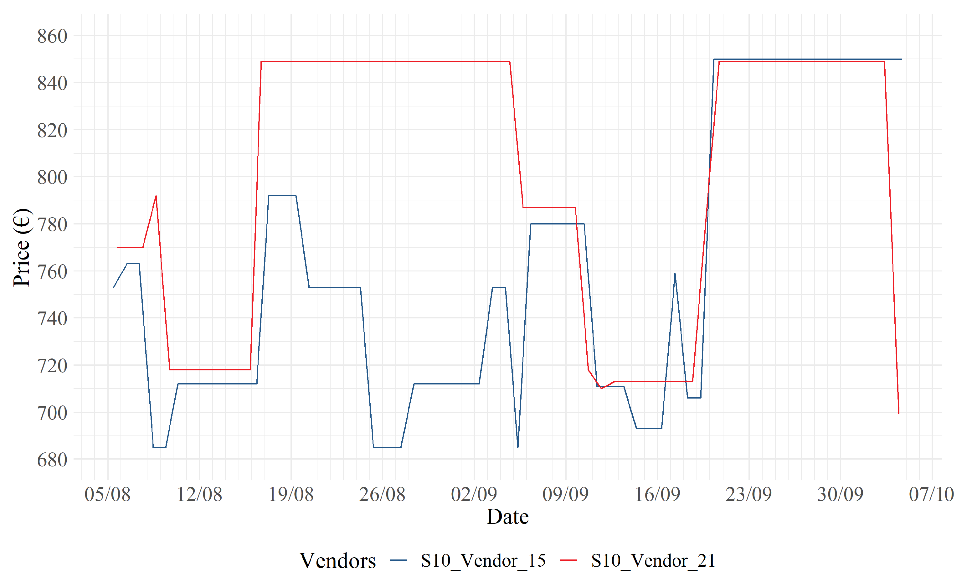
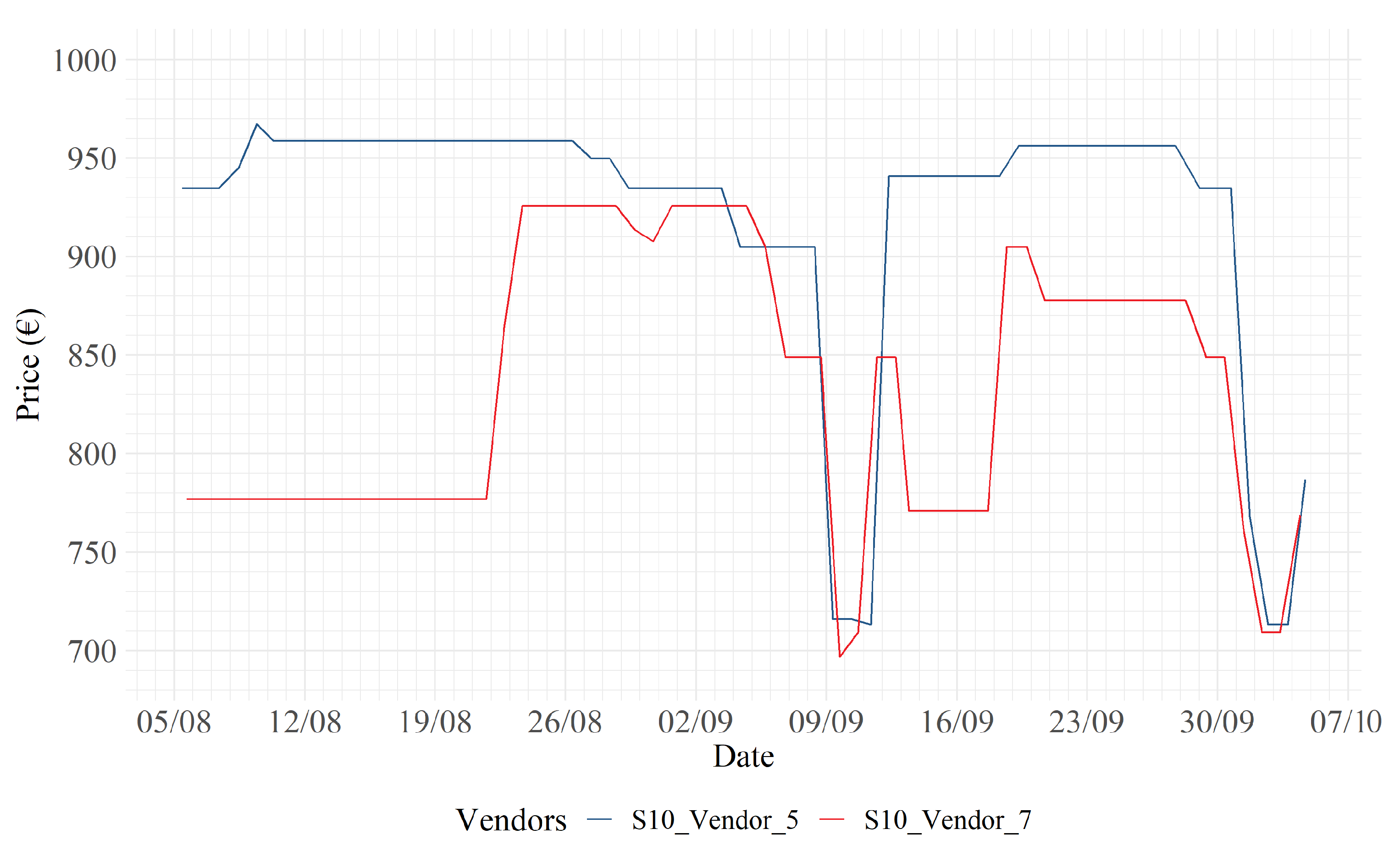
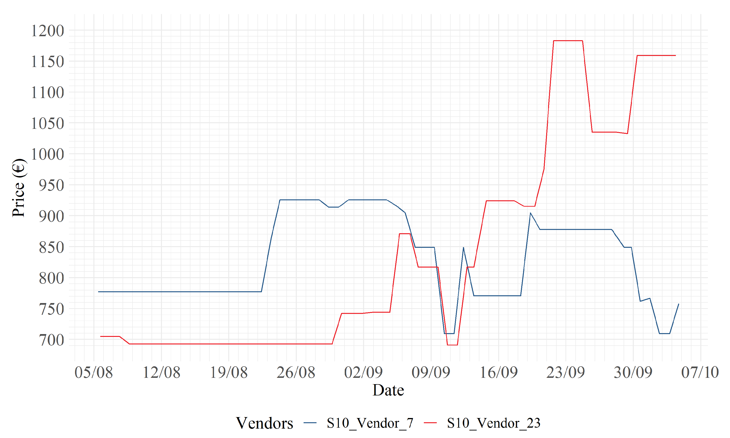
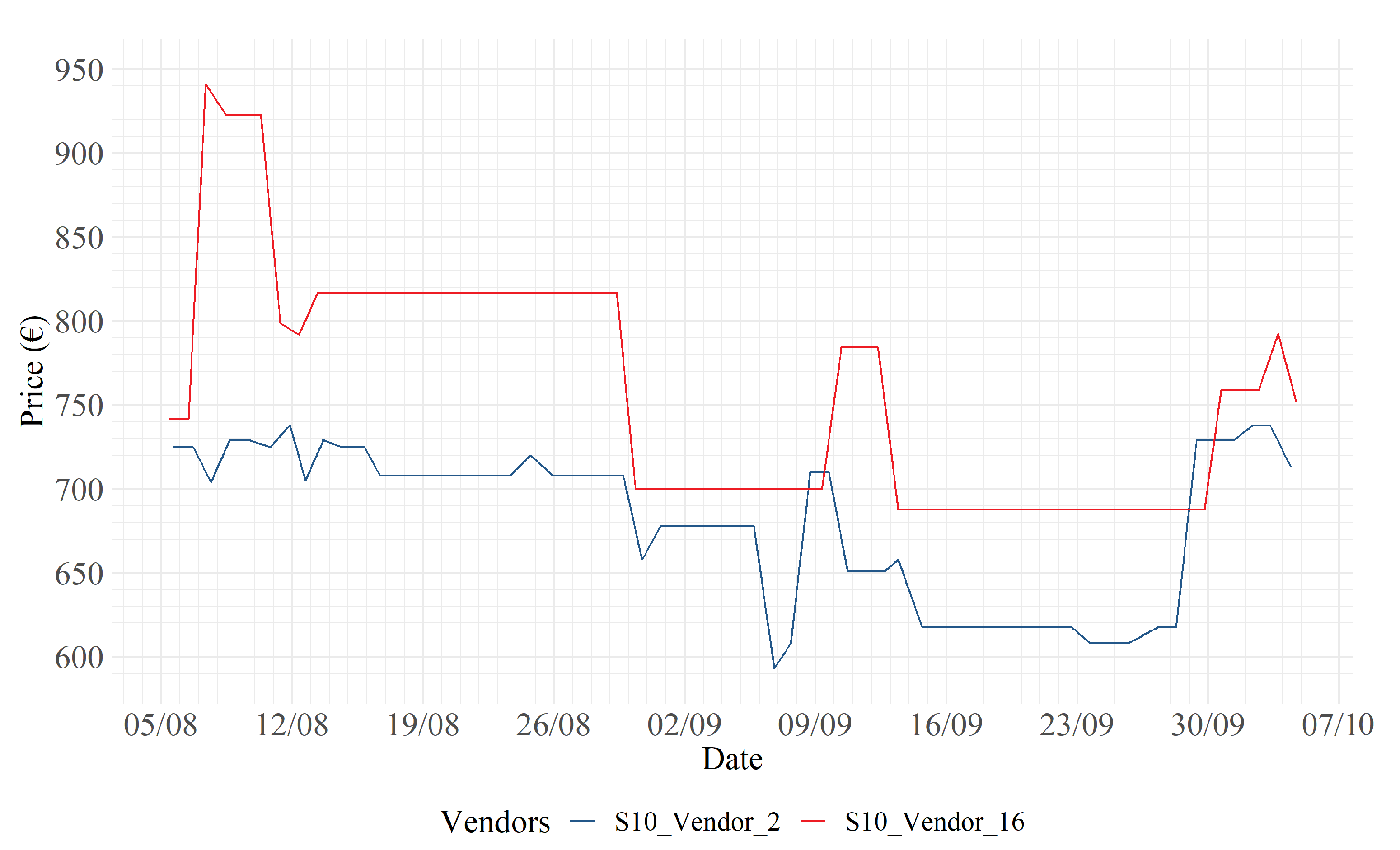
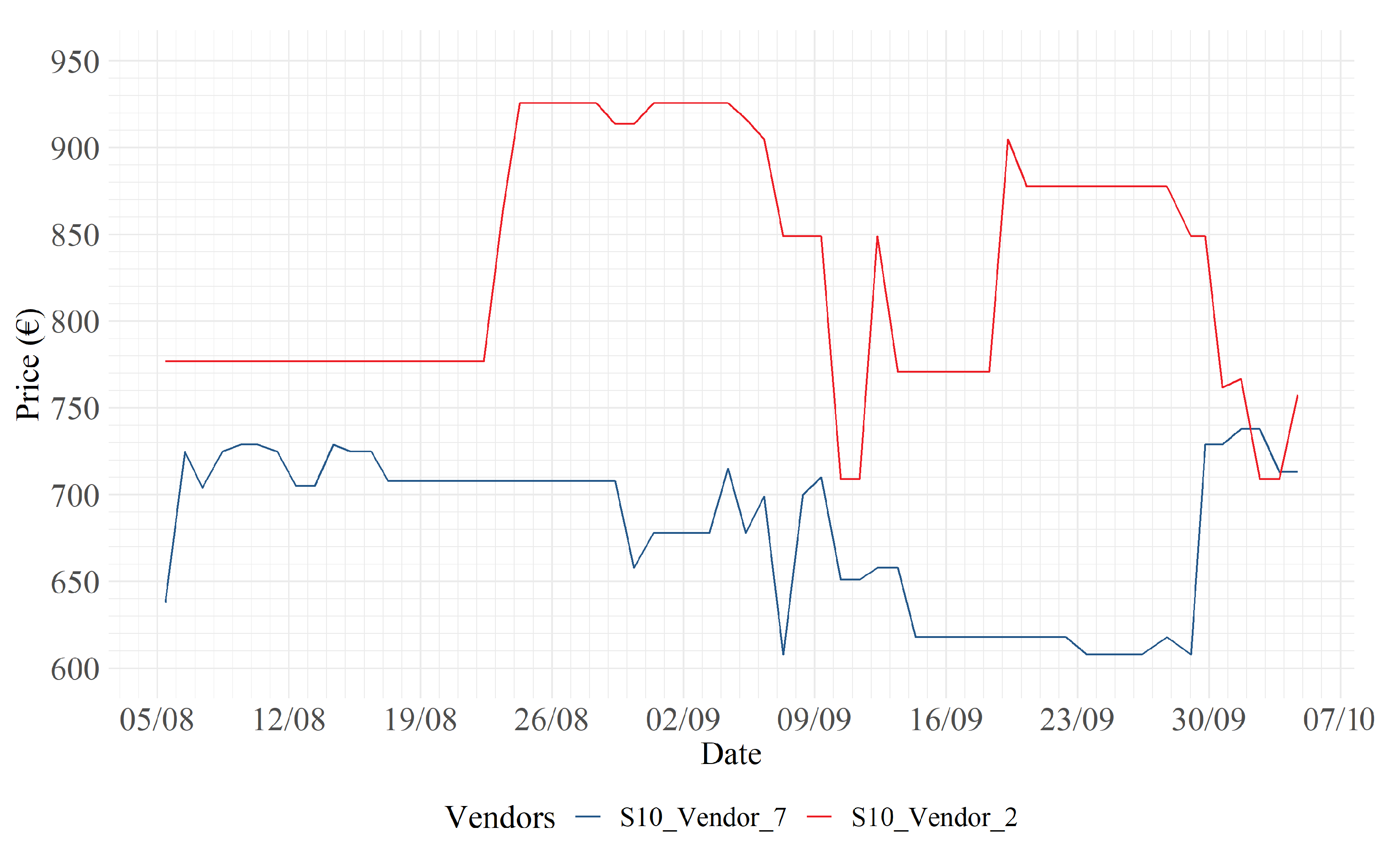
The main purpose of this analysis, performed in an e-commerce environment, was to detect, with a suitable model, dynamic interactions between price variations in time series within close lags. In Figure 7, Figure 8, Figure 9, Figure 10, Figure 11 and Figure 12, six examples of dynamic pricing are shown. The pairs of time series represented are those with the highest values of parameters of the estimated VAR(3) model. The retailers that applied price changes first are in blue, while those reacting to these price changes are in red. Interestingly, all the pairs with significant interactions were related to the Samsung S10. Of the 71 total non-zero parameters of the model, only five were related to time series of the iPhone X and the Huawei P30. This finding appears consistent with the lower variability that characterizes the series related to the iPhone X and Huawei P30 smartphones, as well as the lower price competition at close lags.
In Figure 7, one may observe that retailer 15 (blue) adopts a strategy where a lower price level is maintained with respect to retailer 21 (red). In particular, on August 16, vendor 21 decides to adopt a shadow pricing strategy by increasing its price by approximately 120 EUR. Retailer 15, the next day, responds to this change with a price increase of only 70 EUR, to increase margins on sales, while still maintaining lower price levels with respect to its competitor.
In Figure 8, Figure 9 and Figure 10, it may be noticed that strong price discounts are carried out by the blue vendors on both 9 September and 7 October. Figure 11 displays a dynamic similar to that displayed in Figure 7. In particular, retailer 16 responds to retailer 2’s price increases on 9 and 29 September, with similar increases. In Figure 12 instead there is an interesting and unique dynamic in the dataset: retailer 7 responds to retailer 2’s price increases with opposite reactions. For example, on 29 September, retailer 7 decides to lower its price, in response to an increase by retailer 2, to equalize the price.
The remaining interactions related to non-zero parameters are not displayed because they are less informative in terms of dynamic pricing, although each presented situations where vendors responded to a competitor’s price variations at least once.
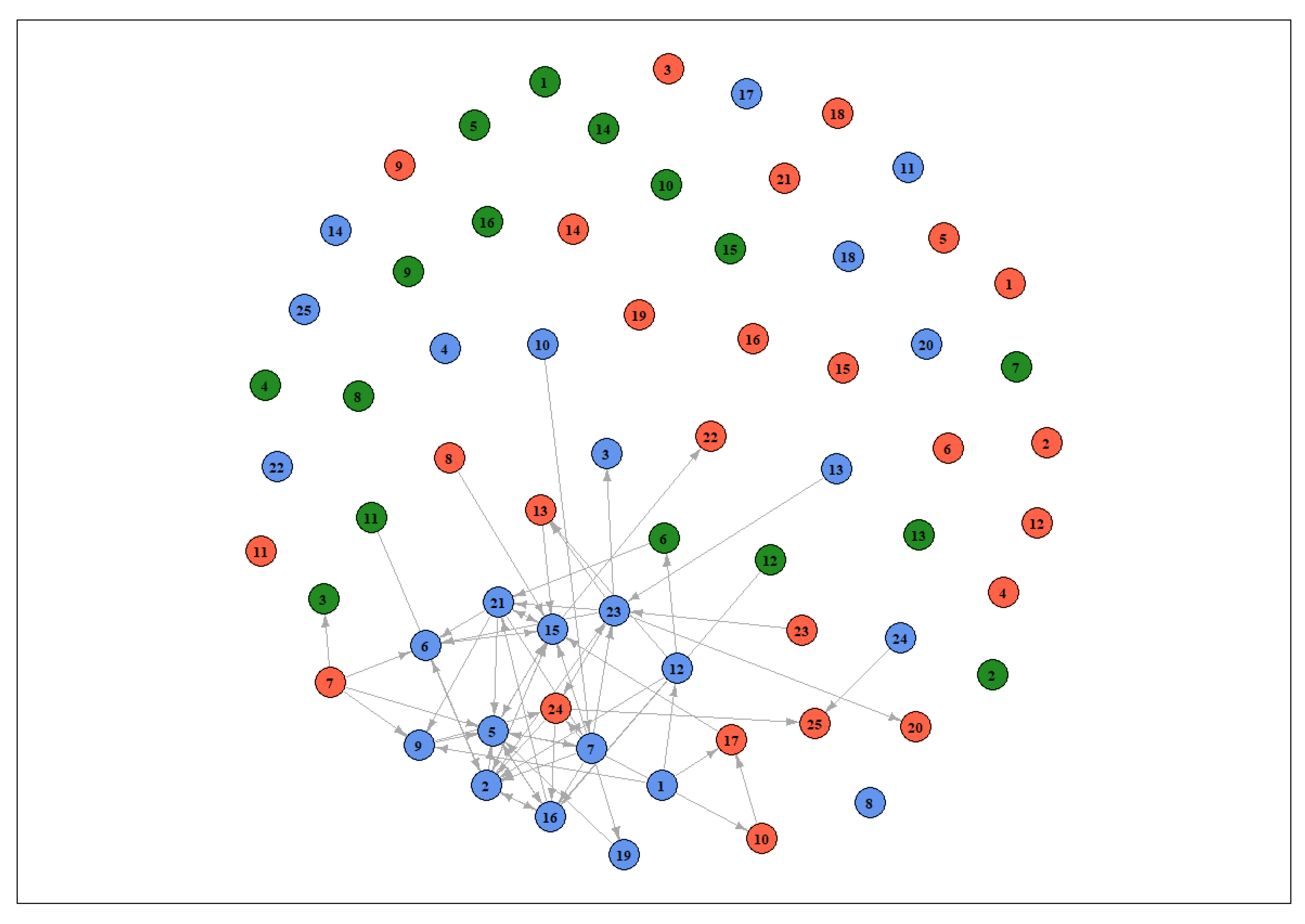
To offer a complete overview of our findings, we show all the relevant relationships detected by the model within the three lags considered (see Figure 6) as a network, displayed in Figure 13. In this network, the dots indicate the 66 vendors and have different colors for identifying the three smartphone models—light blue for Samsung 10, red for Huawei P30 and green for iPhone X—and the links are the dynamic price interactions. From this representation, it may be better appreciated that the e-tailers with a significant strategic interaction with others are a small portion, and most pertain to the Samsung 10, as stated previously. All other nodes do not seem to be characterized by significant relationships. As an interesting insight, the direction of the link indicates “which node influences which”, so that, for example, vendor 1 (Samsung 10) influenced the pricing behavior of vendors 10 and 17 (Huawei P30). Some nodes are especially “linked,” namely, vendors 15, 16, 21 and 23, suggesting the great reactivity of these e-tailers to the pricing behavior of others, and therefore a stronger tendency to perform dynamic pricing strategies. The network representation allowed a simple understanding of dynamic interactions occurring between nodes, showing that most activities involved the Samsung 10, while the iPhone X was not much affected.
7. Final Remarks and Suggestions for Future Research
Through the analysis carried out in this paper, it has been possible to observe how many retailers on e-commerce platforms are careful in monitoring the prices proposed by other manufacturers and, consequently, apply dynamic, shadow and overall competitive pricing strategies. The correct identification of those cases, in which the dynamic interaction actually took place, was possibile by employing a suitable VAR model. The statistical methods adopted in this study may be useful to e-commerce companies that conduct market analyses of competitors’ pricing strategies. In this sense, the more information a company has on the dynamics governing a market and its agents, the greater the company’s competitive advantage over its competitors may be. However, the present findings showed that the number of cases where dynamic pricing was actually observed was not large. This result seems to be in contrast with what one would have expected, given the assumption of the importance of pricing in the marketing mix of e-commerce companies. This may be caused by the limited scope of data retrieval: the more data are available, the more accurately situations of dynamic pricing can be detected.
A major improvement in the analyses carried out could consist, in our opinion, of increasing the granularity of the data observation. For example, observations carried out at shorter intervals (e.g., hourly) would have made it possible to better capture any dynamics of price changes at the very moment they occurred, and consequently, to more accurately identify those cases in which dynamic pricing strategies are actually adopted. Future research could also extend the observation period to capture the long-term development of price competition. In this way, it is assumed that it would also be possible to conduct analyses on the effect of the smartphone’s depreciation over time. A final consideration concerns the choice of the number of different models of smartphones observed. Observing a larger number of smartphones could potentially uncover interesting interdependencies in dynamic price competition across e-commerce vendors.
Author Contributions
Conceptualization, A.F. and M.G.; methodology, A.F. and M.G.; software, A.F.; data curation, A.F.; writing—original draft preparation, A.F. and M.G.; writing—review and editing, A.F. and M.G.; funding acquisition, M.G. All authors have read and agreed to the published version of the manuscript.
Funding
This research was funded by the University of Padua, grant number BIRD188753/18.
Data Availability Statement
The data used in this paper have been collected through the website www.google.com/shopping, from 5 August 2019 to 4 October 2019.
Conflicts of Interest
The authors declare no conflict of interest.
References
- Petropoulos, F.; Apiletti, D.; Assimakopoulos, V.; Babai, M.Z.; Barrow, D.K.; Bergmeir, C.; Ziel, F. Forecasting: Theory and practice. arXiv 2020, arXiv:2012.03854. [Google Scholar]
- Takada, H.; Bass, F.M. Multiple time series analysis of competitive marketing behavior. J. Bus. Res. 1998, 43, 97–107. [Google Scholar] [CrossRef]
- Franses, P.H. Forecasting in marketing. Handb. Econ. Forecast. 2006, 1, 983–1012. [Google Scholar]
- Dekimpe, M.G.; Hanssens, D.M. Time-series models in marketing: Past, present and future. Int. J. Res. Market. 2000, 17, 183–193. [Google Scholar] [CrossRef] [Green Version]
- Hsu, N.J.; Hung, H.L.; Chang, Y.M. Subset selection for vector autoregressive processes using Lasso. Comput. Stat. Data Anal. 2008, 52, 3645–3657. [Google Scholar] [CrossRef]
- Tibshirani, R. Regression Shrinkage and Selection via the Lasso. J. R. Stat. Soc. 1996, 58, 267–288. [Google Scholar] [CrossRef]
- Nicholson, W.B.; Wilms, I.; Bien, J.; Matteson, D.S. High dimensional forecasting via interpretable vector autoregression. J. Mach. Learning Res. 2020, 21, 1–52. [Google Scholar]
- Gelper, S.; Wilms, I.; Croux, C. Identifying demand effects in a large network of product categories. J. Retail. 2016, 92, 25–39. [Google Scholar] [CrossRef] [Green Version]
- Ma, S.; Fildes, R.; Huang, T. Demand forecasting with high dimensional data: The case of SKU retail sales forecasting with intra-and inter-category promotional information. Eur. J. Op. Res. 2016, 249, 245–257. [Google Scholar] [CrossRef] [Green Version]
- Fildes, R.; Ma, S.; Kolassa, S. Retail forecasting: Research and practice. Int. J. Forecast. 2019, in press. [Google Scholar] [CrossRef] [Green Version]
- Kotler, P.; Keller, K.L. Marketing Management; Pearson: London, UK, 2012. [Google Scholar]
- McCarthy, J. Basic Marketing, A Managerial Approach; R. D. Irwin: Homewood, CA, USA, 1960. [Google Scholar]
- Sims, C.A. Macroeconomics and reality. Econ. J. Econ. Soc. 1980, 1–48. [Google Scholar] [CrossRef] [Green Version]
- Lütkepohl, H. New Introduction To Time Series Analysis; Springer: New York, NY, USA, 2005. [Google Scholar]
- Tsay, R. Multivariate Time Series Analysis: With R and Financial Applications; John Wiley & Sons, Inc.: London, UK, 2014. [Google Scholar]
- Azzalini, A.; Scarpa, B. Data Analysis and Data Mining: An Introduction; Oxford University Press: Oxford, UK, 2012. [Google Scholar]
- Salkind, N.J. Encyclopedia of Research Design; Sage Publications: Thousand Oaks, CA, USA, 2010; Volume 1. [Google Scholar]
- Cheung, Y.W.; Lai, K.S. Lag order and critical values of the augmented Dickey–Fuller test. J. Bus. Econ. Stat. 1995, 13, 277–280. [Google Scholar]
- Nicholson, W.; Matteson, D.; Bien, J. BigVAR: Dimension Reduction Methods for Multivariate Time Series; R package version 1.0.4. 2019. Available online: https://CRAN.R-project.org/package=BigVAR (accessed on 15 October 2019).
Figure 1.
Number of time series available before data cleaning.

Figure 2.
Observed smartphone prices.

Figure 3.
Transformed data for Huawei P30.

Figure 4.
Transformed data for Samsung S10.

Figure 5.
Transformed data for Apple iPhone X.

Figure 6.
matrices for lags of the estimated model.

Figure 7.
S10: 15 (blue) vs. 21 (red).

Figure 8.
S10: 5 (blue) vs. 7 (red).

Figure 9.
S10: 7 (blue) vs. 23 (red).

Figure 10.
S10: 9 (blue) vs. 5 (red).

Figure 11.
S10: 2 (blue) vs. 16 (red).

Figure 12.
S10: 7 (blue) vs. 2 (red).

Figure 13.
Dynamic pricing as a network: The dots are vendors, and the links are dynamic pricing interactions.
Figure 13.
Dynamic pricing as a network: The dots are vendors, and the links are dynamic pricing interactions.


Table 1.
Summary statistics for iPhone X, Huawei P30 and Samsung S10.
| Smartphone | Num. of Vendors | Minimum | Mean | Maximum | Std. Dev. | |
|---|---|---|---|---|---|---|
| 1 | iPhone X | 16 | −5.08 | 0.02 | 5.05 | 0.46 |
| 2 | Huawei P30 | 25 | −5.27 | −0.01 | 5.30 | 0.63 |
| 3 | Samsung S10 | 25 | −5.25 | −0.00 | 5.43 | 0.98 |
Publisher’s Note: MDPI stays neutral with regard to jurisdictional claims in published maps and institutional affiliations. |
© 2021 by the authors. Licensee MDPI, Basel, Switzerland. This article is an open access article distributed under the terms and conditions of the Creative Commons Attribution (CC BY) license (http://creativecommons.org/licenses/by/4.0/).
Share and Cite
MDPI and ACS Style
Faehnle, A.; Guidolin, M. Dynamic Pricing Recognition on E-Commerce Platforms with VAR Processes. Forecasting 2021, 3, 166-180. https://0-doi-org.brum.beds.ac.uk/10.3390/forecast3010011
AMA Style
Faehnle A, Guidolin M. Dynamic Pricing Recognition on E-Commerce Platforms with VAR Processes. Forecasting. 2021; 3(1):166-180. https://0-doi-org.brum.beds.ac.uk/10.3390/forecast3010011
Chicago/Turabian StyleFaehnle, Alexander, and Mariangela Guidolin. 2021. "Dynamic Pricing Recognition on E-Commerce Platforms with VAR Processes" Forecasting 3, no. 1: 166-180. https://0-doi-org.brum.beds.ac.uk/10.3390/forecast3010011