Modeling of Lake Malombe Annual Fish Landings and Catch per Unit Effort (CPUE)

 ,
, 
 , and
, and
Abstract
:1. Introduction
2. Materials and Methods
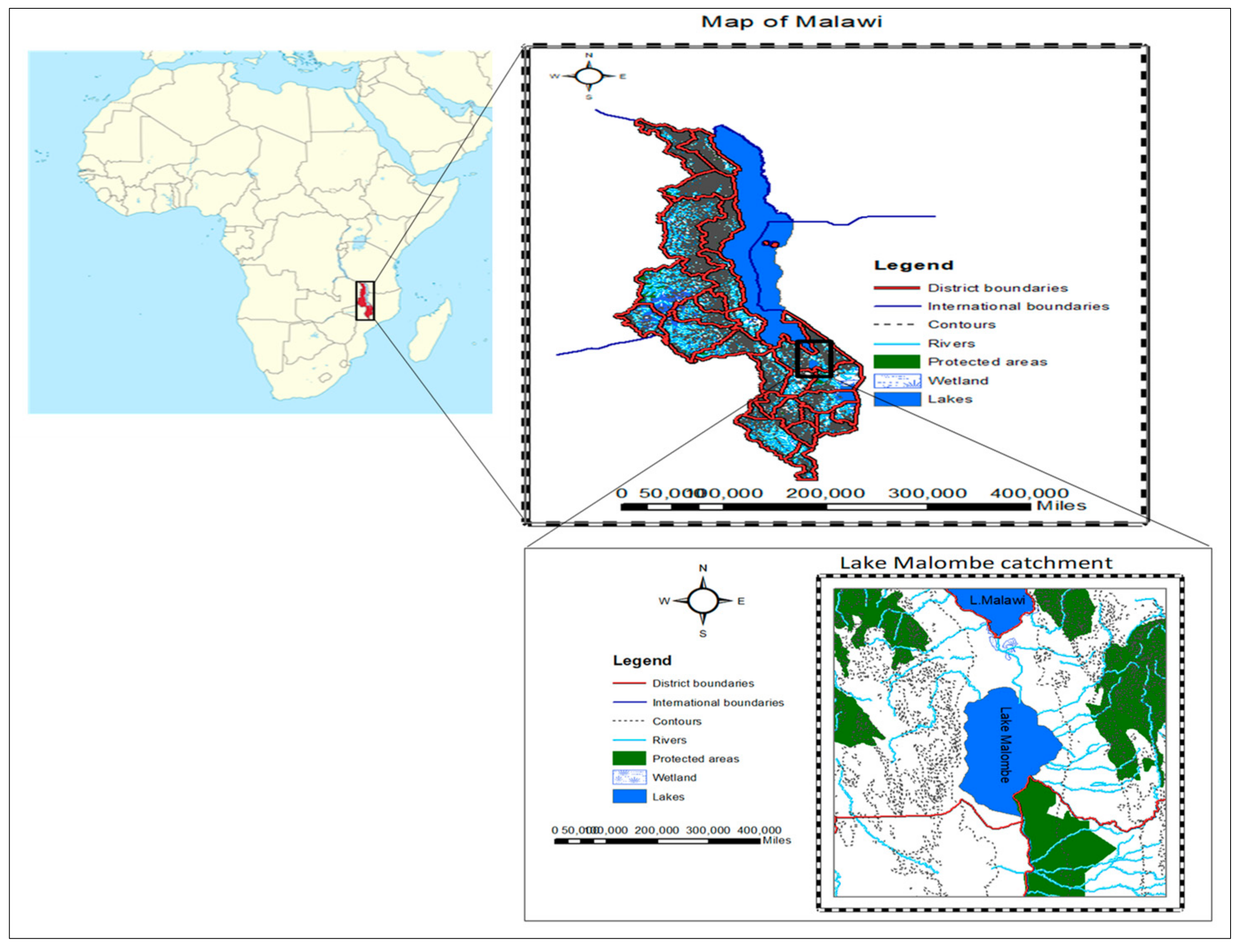
2.1. The Study Area
2.2. Data Sources
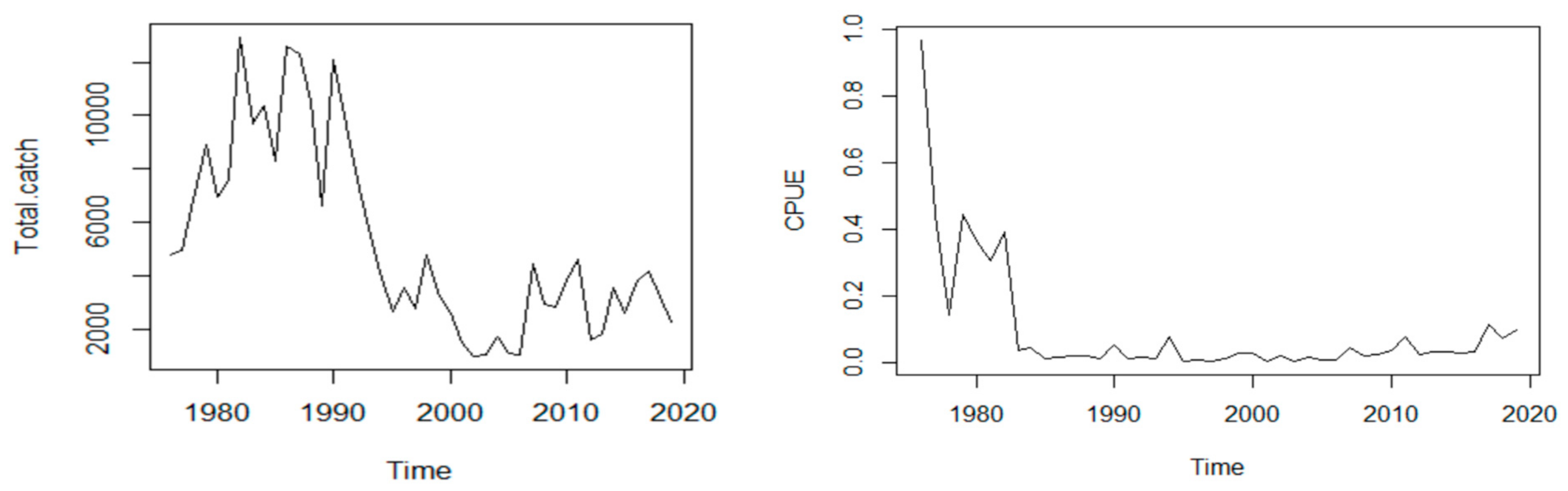
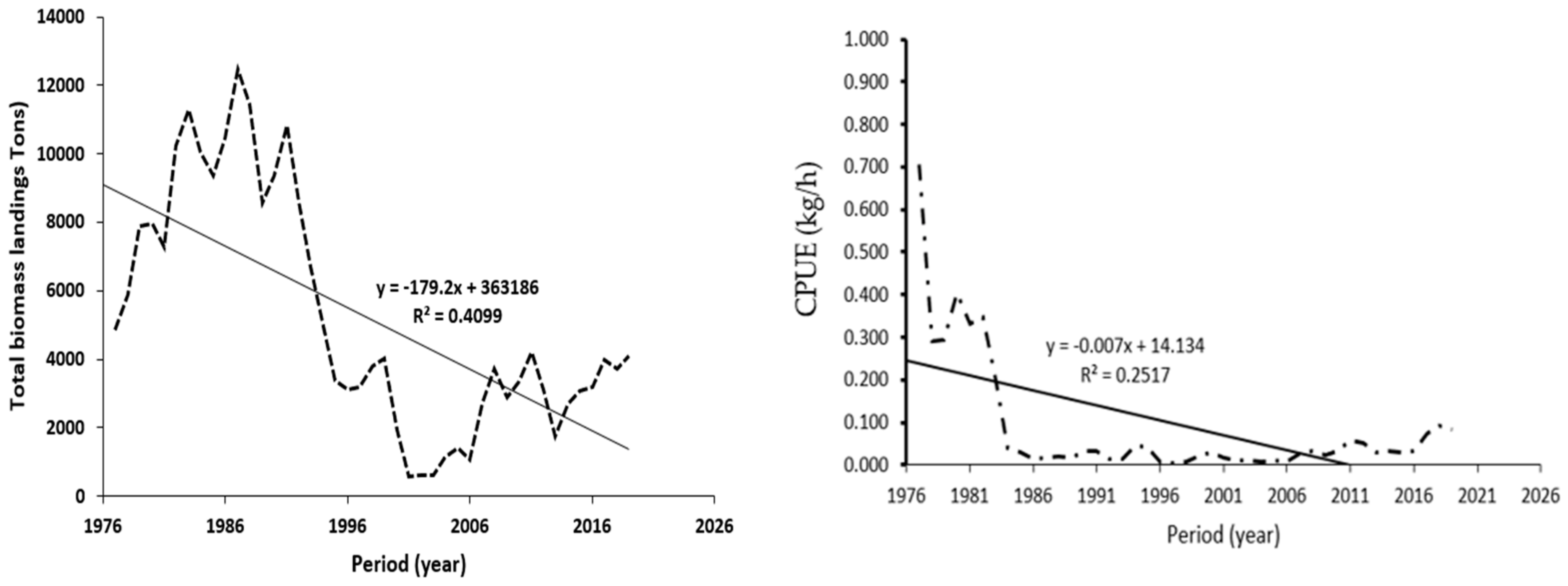
2.2.1. Fish Biomass
2.2.2. The Estimation of Catch per Unit Effort (CPUE)
2.2.3. Conceptual Framework of the ARIMA Model
3. Results
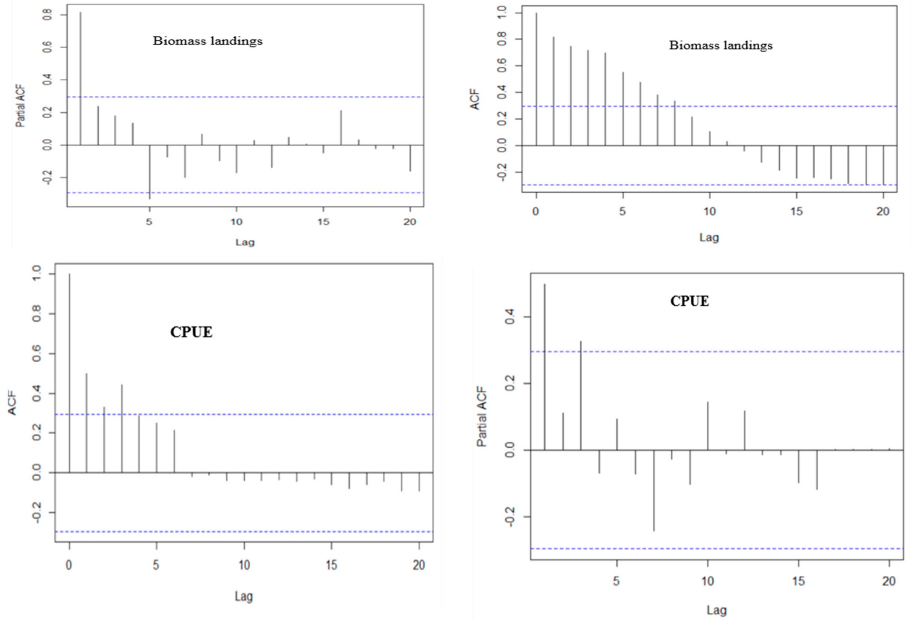
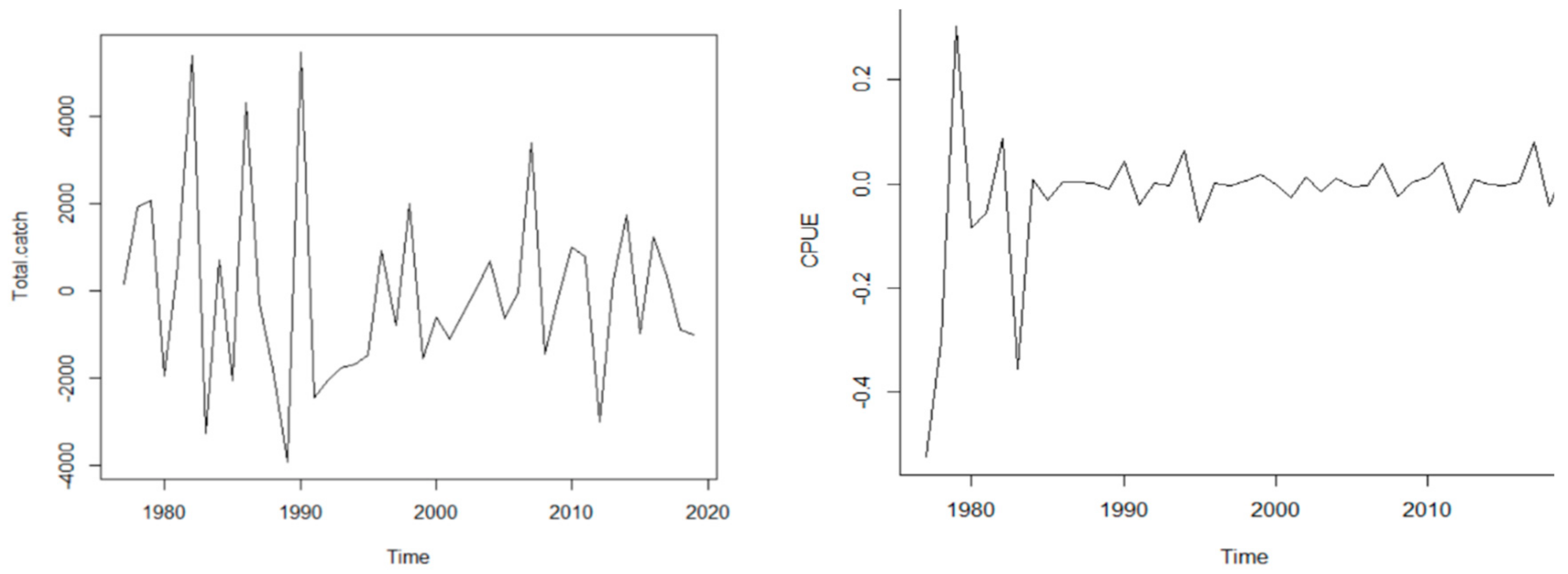
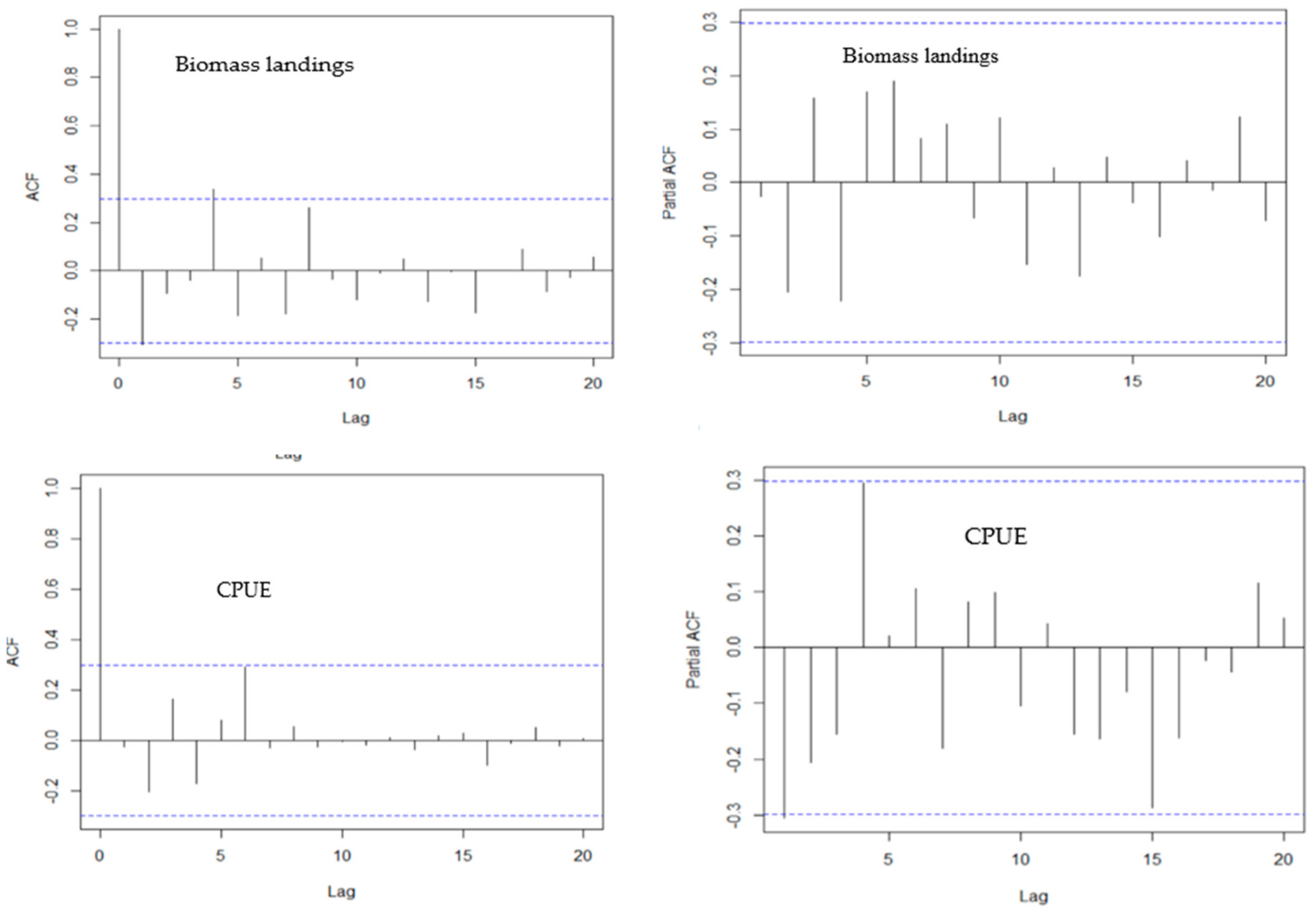
3.1. Model Identification
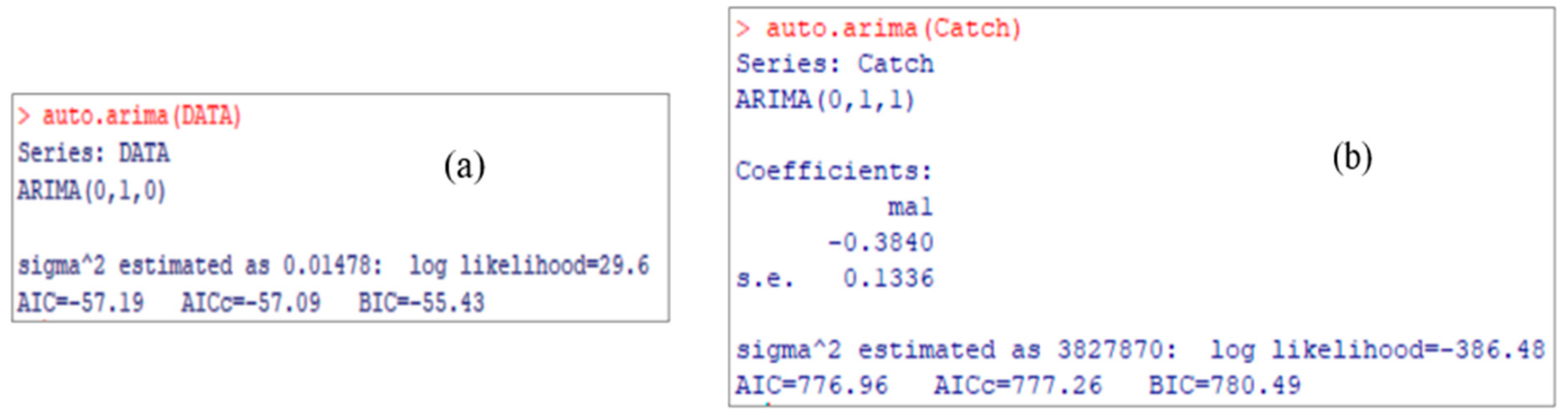
3.2. Model Selection
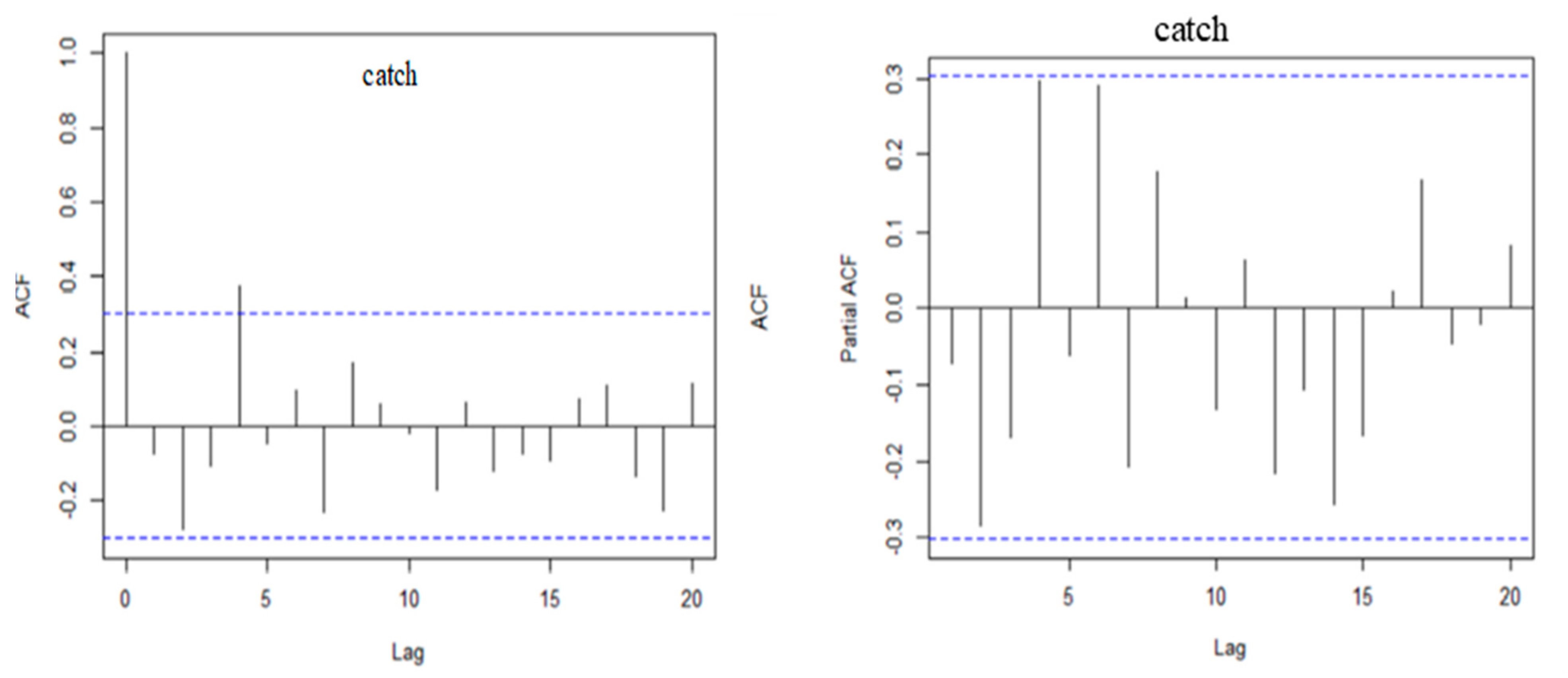
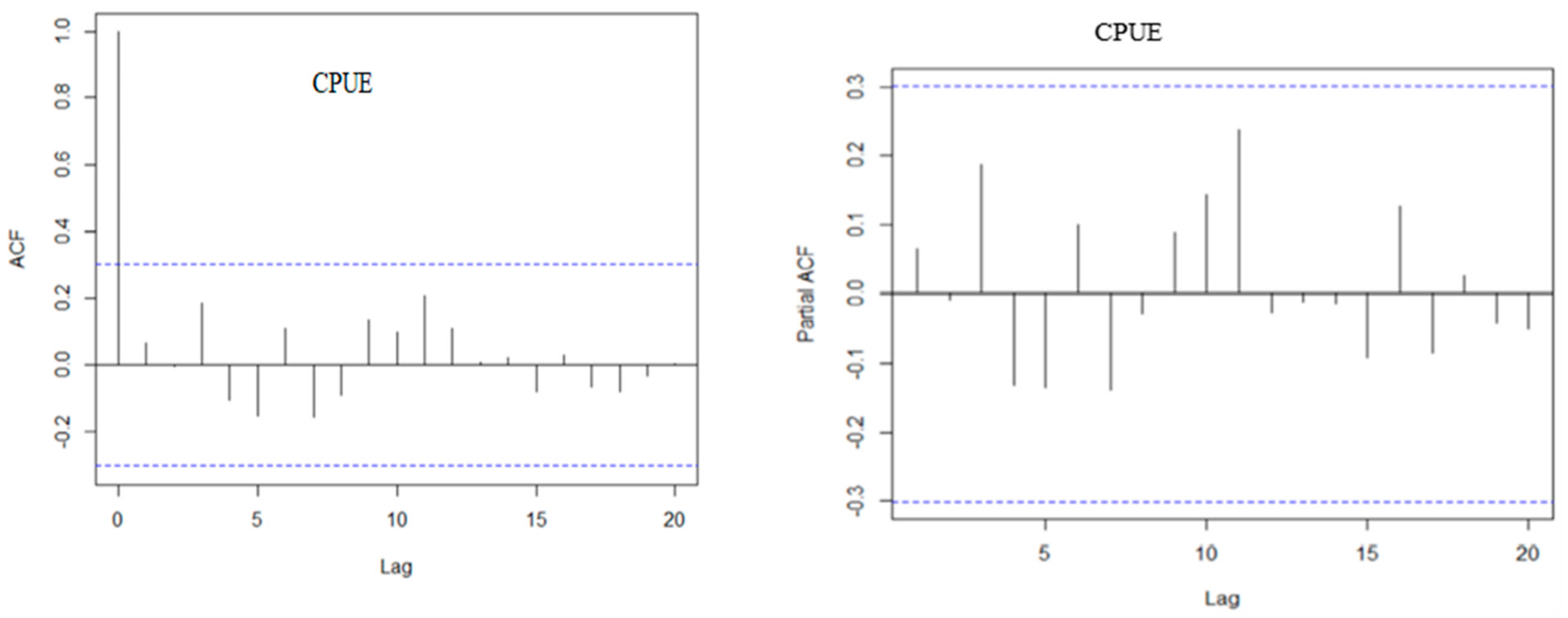
3.3. Accuracy of ARIMA (0,1,1) and ARIMA (0,1,0) Models
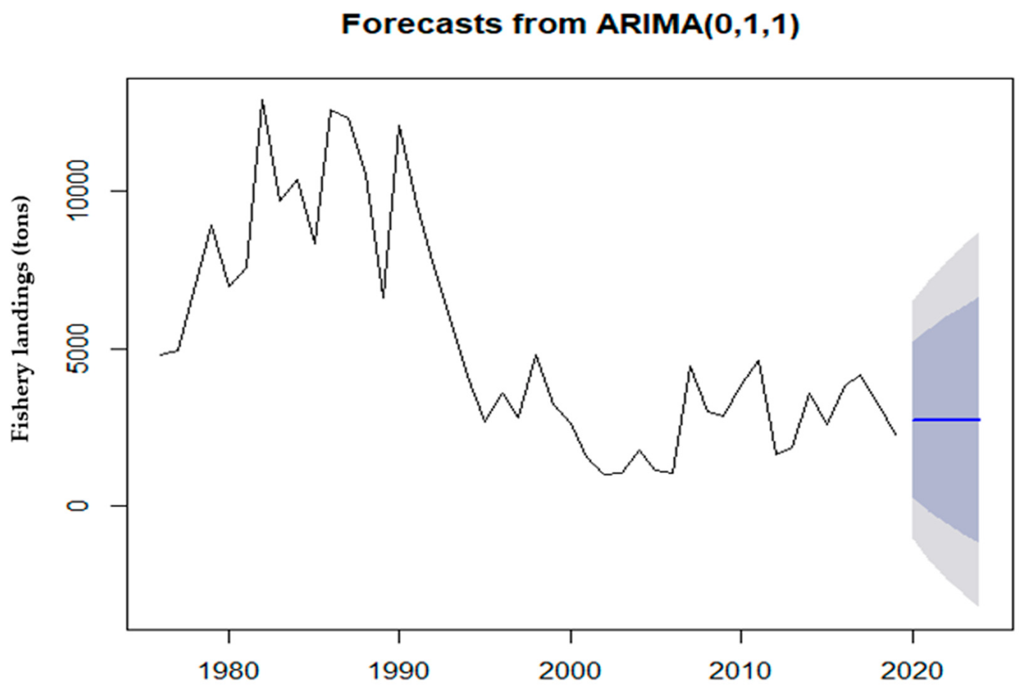
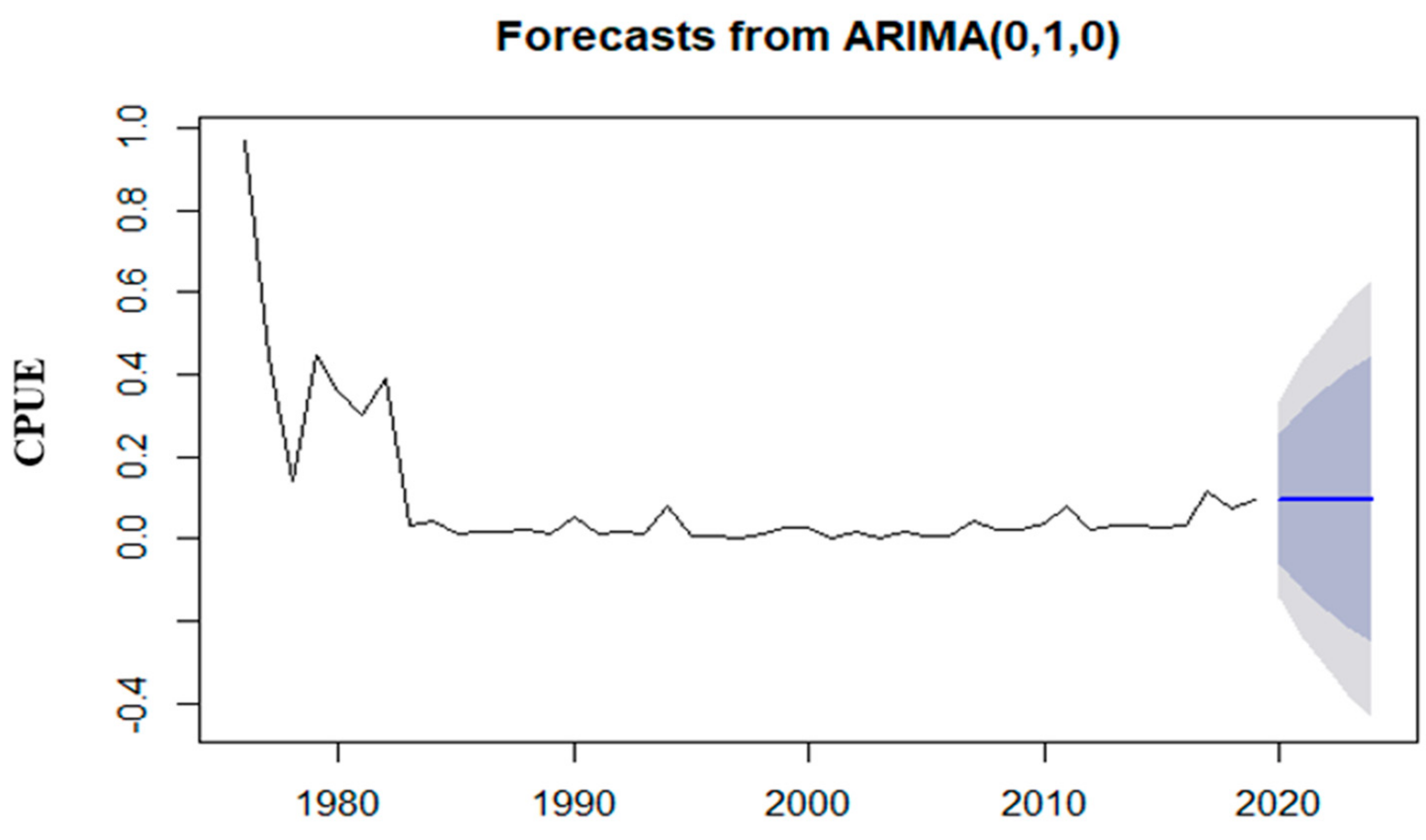
4. Forecast
5. Discussion
6. Conclusions
7. Limitation
Author Contributions
Funding
Institutional Review Board Statement
Informed Consent Statement
Acknowledgments
Conflicts of Interest
References
- Weyl, O.L.F.; Ribbink, A.J.; Tweddle, D. Lake Malawi: Fishes, fisheries, biodiversity, health and habitat. Aquat. Ecosyst. Health Manag. 2010, 13, 241–254. [Google Scholar] [CrossRef]
- Hara, M.; Njaya, F. Between a rock and a hard place: The need for and challenges to implementation of Rights Based Fisheries Management in small-scale fisheries of southern Lake Malawi. Fish. Res. 2016, 174, 10–18. [Google Scholar] [CrossRef] [Green Version]
- Government of Malawi. Fisheries Conservation and Management Act; Malawi Government: Lilongwe, Malawi, 1997.
- Hara, M.; Nielsen, J.R. Experiences with Fisheries Co-Management in Africa; Wilson, D.C., Nielsen, J.R., Degnbol, P., Eds.; Springer Nature: Dordrecht, The Netherdlands, 2003; pp. 81–97. [Google Scholar]
- Hara, M. Community response: Decline of the chambo in lake Malawi’s southeast arm. In Poverty Mosaics: Realities and Prospects in Small-Scale Fisheries; Jentoft, S., Eide, A., Eds.; Springer Science & Business Media B.V.: Berlin, Germany, 2011. [Google Scholar] [CrossRef]
- Njaya, F. Governance challenges for the implementation of co-management: Experiences from Malawi. Int. J. Commons 2007, 1, 137–153. [Google Scholar] [CrossRef]
- Lewy, P.; Nielsen, A. Modelling stochastic fish stock dynamics using Markov Chain Monte Carlo. ICES J. Mar. Sci. 2003, 60, 743–752. [Google Scholar] [CrossRef] [Green Version]
- Craine, M. Modelling Western Australian Fisheries with Techniques of Time Series Analysis: Examining Data from a Different Perspective; Department of Fisheries Research Division, Western Australian Marine Research Laboratories: North Beach, Australia, 2005. [Google Scholar]
- Stergiou, K. Prediction of the Mullidae fishery in the eastern Mediterranean 24 months in advance. Fish. Res. 1990, 9, 67–74. [Google Scholar] [CrossRef]
- Selvaraj, J.J.; Arunachalam, V.; Coronado-Franco, K.V.; Romero-Orjuela, L.V.; Ramírez-Yara, Y.N. Time-series modeling of fishery landings in the Colombian Pacific Ocean using an ARIMA model. Reg. Stud. Mar. Sci. 2020, 39, 101477. [Google Scholar] [CrossRef]
- Koutroumanidis, T.; Iliadis, L.; Sylaios, G.K. Time-series modeling of fishery landings using ARIMA models series modeling of fishery landings using ARIMA models. Environ. Model. Softw. 2006, 21, 1711–1721. [Google Scholar] [CrossRef]
- Park, H.-H. Analysis and prediction of walleye pollock (Theragra chalcogramma) landings in Korea by time series analysis. Fish. Res. 1998, 38, 1–7. [Google Scholar] [CrossRef]
- Georgakarakos, S.; Koutsoubas, D.; Valavanis, V.D. Time series analysis and forecasting techniques applied on loliginid and ommastrephid landings in Greek waters. Fish. Res. 2006, 78, 55–71. [Google Scholar] [CrossRef] [Green Version]
- Lloret, J.; Lleonart, J.; Solé, I. Time series modelling of landings in Northwest Mediterranean Sea. ICES J. Mar. Sci. 2000, 57, 171–184. [Google Scholar] [CrossRef] [Green Version]
- Prista, N.; Diawara, N.; Costa, M.J.; Jones, C.M. Use of SARIMA models to assess data-poor fisheries: A case study with sciaenid fishery of Portugal. Fish Bull. 2011, 109, 170–182. [Google Scholar]
- Raman, R.K.; Sathianandan, T.V.; Sharma, A.P.; Mohanty, B.P. Modelling and forecasting marine fish production in Odisha using seasonal ARIMA model. Natl. Acad. Sci. Lett. 2017, 40, 393–397. [Google Scholar] [CrossRef]
- Stergiou, K.I. Modelling and forecasting the fishery for pilchard (Sardina pilchardus) in Greek waters using ARIMA time-series models. ICES J. Mar. Sci. 1989, 46, 16–23. [Google Scholar] [CrossRef]
- Dulanya, Z.; Croudace, I.; Reed, J.M.; Trauth, M.H. Palaeoliminological reconstruction of recent environmental change in Lake Malombe (S.Malawi) using multiple proxies. Water SA 2014, 40, 1–12. [Google Scholar] [CrossRef] [Green Version]
- Matiya, G.; Wakabayashi, Y. Small scale fisheries of Malawi: An outline of Lake Malombe fisheries. Mem. Fac. Agric. Ehime Univ. 2005, 50, 3–9. [Google Scholar]
- Petrere, M., Jr.; Giacomini, H.C.; De Marco, P., Jr. Catch-per-unit-effort: Which estimator is best? Braz. J. Biol. 2010, 70, 483–491. [Google Scholar] [CrossRef] [PubMed] [Green Version]
- Thompson, S.K. Sampling; Wiley: New York, NY, USA, 1992. [Google Scholar]
- Griffiths, R.C. A study of measures of population density and the concentration of fishing effort in the fishery for yellowfin tuna, Neothunnus macropterous, in the Eastern tropical Pacific Ocean, from 1951 to 1956. Inter-Am. Trop. Tuna Comm. Bull. 1960, 4, 41–96. [Google Scholar]
- Snedecor, G.W.; Cochran, W.G. Statistical Methods, 6 ed.; The Iowa State University Press: Ames, IA, USA, 1967. [Google Scholar]
- Gutiérrez-Estrada, J.C.; Silva, C.; Yáñez, E.; Rodríguez, N.; Pulido-Calvo, I. Monthly catch forecasting of anchovy Engraulis ringens in the north area of Chile: Non-linear univariate approach. Fish. Res. 2007, 86, 188–200. [Google Scholar] [CrossRef]
- Makwinja, R.; Singini, W.; Kaunda, E.; Kapute, F.; M’balaka, M. Stochastic modeling of Lake Malawi Engraulicypris sardella (Gunther, 1868) catch fluctuation. Int. J. Fish. Aquac. 2018, 10, 34–43. [Google Scholar]
- Box, G.E.P.; Jenkins, G.M. Time Series Analysis: Forecasting and Control.; Holden Day: Oakland, CA, USA, 1976. [Google Scholar]
- Mgaya, J.F.; Yildiz, F. Application of ARIMA models in forecasting livestock products consumption in Tanzania. Cogent Food Agric. 2019, 5, 1607430. [Google Scholar] [CrossRef]
- Harley, S.J.; Ransom, A.M.; Dunn, A. Is catch-per-unit-effort proportional to abundance? Can. J. Fish. Aquat. Sci. 2001, 58, 1760–1772. [Google Scholar] [CrossRef]
- Guzzo, M.M.; Rennie, M.D.; Blanchfield, P.J. Evaluating the relationship between mean catch per unit effort and abundance for littoral cyprinids in small boreal shield lakes. Fish. Res. 2014, 150, 100–108. [Google Scholar] [CrossRef]
- Maynou, F.; Demetre, M.; Sánchez, P. Analysis of catch per unit effort by multivariate analysis and generalized linear models for deep-water crustacean fisheries off Barcelona (NW Mediterranean). Fish. Res. 2003, 65, 257–269. [Google Scholar] [CrossRef]
- Weyl, O.; Mwakiyongo, K.; Mandere, D. An assessment of the nkacha net fishery of Lake Malombe Malawi. Afr. J. Aquat. Sci. 2004, 29, 47–55. [Google Scholar] [CrossRef]
- El-Far, A.; Aly, W.; El-Haweet, A.E.-D.; Nasr-Allah, A.; Karisa, H. Fisheries management based on gear selectivity of a tropical reservoir, Lake Nasser, Egypt. Egypt. J. Aquat. Res. 2020, 46, 71–77. [Google Scholar] [CrossRef]
- Solomon, S.G.; Ayuba, V.O.; Tahir, M.A.; Okomoda, V.T. Catch per unit effort and some water quality parameters of Lake Kalgwai Jigawa state, Nigeria. Food Sci. Nutr. 2018, 6, 450–456. [Google Scholar] [CrossRef] [Green Version]
- Alexander, T.J.; Vonlanthen, P.; Periat, G.; Degiorgi, F.; Raymond, J.; Seehausen, O. Estimating whole-lake fish catch per unit effort. Fish. Res. 2015, 172, 287–302. [Google Scholar] [CrossRef]
- Kidd, K.A.; Blanchfield, P.J.; Mills, K.H.; Palace, V.P.; Evans, R.E.; Lazorchak, J.M.; Flick, R.W. Collapse of a fish population after exposure to a synthetic estrogen. Proc. Natl. Sci. USA 2007, 104, 8897–8901. [Google Scholar] [CrossRef] [PubMed] [Green Version]
- Njaya, F.; Snyder, K.A.; Jamu, D.; Wilson, J.; Howard-Williams, C.; Allison, E.H.; Andrew, N.L. The natural history and fisheries ecology of Lake Chilwa, southern Malawi. J. Great Lakes Res. 2011, 37, 15–25. [Google Scholar] [CrossRef]
- Makwinja, R.; Chapotera, M.; Likongwe, P.; Banda, J.; Chijere, A. Location and roles of deep pools in Likangala river during 2012 recession period of Lake Chilwa basin. Int. J. Ecol. 2014, 2014, 1–4. [Google Scholar] [CrossRef] [Green Version]
- Stergiou, K.I. Overfishing, the tropicalization of fish stocks, uncertainty, and ecosystem management: Resharpening Ockham’s razor. Fish. Res. 2002, 55, 1–9. [Google Scholar]
- Pinnegar, J.K.; Polunin, N.V.C.; Badalamenti, F. Long-term changes in the trophic level of western Mediterranean fishery and aquaculture landings. Can. J. Fish. Aquat. Sci. 2003, 60, 222–235. [Google Scholar] [CrossRef]
- FAO. Fisheries Management; FAO Technical Guidelines for Responsible Fisheries. No. 4; Food and Agriculture Organization of the United Nations: Rome, Italy, 1997. [Google Scholar]


| Model (p,d,q) | R2 | RMSE (tons) | MAE (tons) | BIC | AIC | Log-Likelihood | SEP (%) | ARV | E2 | PI | Ljung–Box (p-Value) |
|---|---|---|---|---|---|---|---|---|---|---|---|
| ARIMA (0,1,0) | 0.69 | 2035.37 | 1507.99 | 815.50 | 777.96 | −386.49 | 32 | 0.33 | 0.67 | 0.23 | 0.49 |
| ARIMA (1,1,1) | 0.69 | 2035.24 | 1514.83 | 795.50 | 778.95 | −389.48 | 44 | 0.33 | 0.67 | 0.13 | 0.63 |
| ARIMA (2,1,2) | 0.69 | 2067.42 | 1518.65 | 795.61 | 779.60 | −386.76 | 56 | 0.34 | 0.66 | 0.14 | 0.89 |
| ARIMA (2,2,2) | 0.70 | 2107.42 | 1494.62 | 815.83 | 777.65 | −398.82 | 53 | 0.35 | 0.65 | 0.44 | 0.48 |
| ARIMA (0,1,1) | 0.73 | 2001.29 | 1044.04 | 780.49 | 776.96 | −386.48 | 22 | 0.29 | 0.71 | 0.56 | 0.64 |
| ARIMA (2,0,0) | 0.66 | 2015.74 | 1474.24 | 915.06 | 788.68 | −389.34 | 76 | 0.32 | 0.68 | 0.39 | 0.65 |
| Model (p,d,q) | R2 | RMSE (kg/h) | MAE (kg/h) | BIC | AIC | Log-Likelihood | SEP (%) | ARV | E2 | PI | Ljung–Box (p-Value) |
|---|---|---|---|---|---|---|---|---|---|---|---|
| ARIMA (0,1,0) | 0.75 | 0.08 | 0.05 | −55.43 | −57.19 | 39.6 | 26 | 0.25 | 0.6465 | 0.66 | 0.589 |
| ARIMA (1,1,1) | 0.74 | 0.11 | 0.06 | −44.08 | −53.68 | 29.84 | 44 | 0.37 | 0.6264 | 0.38 | 0.844 |
| ARIMA (2,1,2) | 0.72 | 0.10 | 0.06 | −47.09 | −55.67 | 34.84 | 47 | 0.39 | 0.6057 | 0.29 | 0.707 |
| ARIMA (2,2,2) | 0.57 | 0.12 | 0.07 | −45.08 | −54.88 | 32.44 | 64 | 0.36 | 0.6398 | 0.47 | 0.717 |
| ARIMA (0,1,1) | 0.75 | 0.11 | 0.06 | −49.14 | −43.94 | 24.97 | 54 | 0.43 | 0.5701 | 0.32 | 0.787 |
| ARIMA (2,0,0) | 0.75 | 0.13 | 0.07 | −36.68 | −42.54 | −35.34 | 92 | 0.43 | 0.5700 | 0.34 | 0.645 |
| Year | Forecast | Lo 80 | Hi 80 | Lo 95 | Hi 95 |
|---|---|---|---|---|---|
| 2020 | 2725.243 | 147.222 | 5203.265 | −1064.563 | 6515.05 |
| 2021 | 2725.243 | −185.147 | 5635.634 | −1725.814 | 7176.301 |
| 2022 | 2725.243 | −561.115 | 6011.602 | −2300.809 | 7751.295 |
| 2023 | 2725.243 | −898.282 | 6348.769 | −2816.460 | 8266.947 |
| 2024 | 2725.243 | −1206.64 | 6657.128 | −3288.055 | 8738.542 |
| Year | Forecast | Lo 80 | Hi 80 | Lo 95 | Hi 95 |
|---|---|---|---|---|---|
| 2020 | 0.097 | −0.059 | 0.252 | −0.141 | 0.335 |
| 2021 | 0.097 | −0.123 | 0.317 | −0.240 | 0.434 |
| 2022 | 0.097 | −0.173 | 0.367 | −0.316 | 0.509 |
| 2023 | 0.097 | −0.215 | 0.409 | −0.380 | 0.574 |
| 2024 | 0.097 | −0.251 | 0.445 | −0.436 | 0.629 |
Publisher’s Note: MDPI stays neutral with regard to jurisdictional claims in published maps and institutional affiliations. |
© 2021 by the authors. Licensee MDPI, Basel, Switzerland. This article is an open access article distributed under the terms and conditions of the Creative Commons Attribution (CC BY) license (http://creativecommons.org/licenses/by/4.0/).
Share and Cite
Makwinja, R.; Mengistou, S.; Kaunda, E.; Alemiew, T.; Phiri, T.B.; Kosamu, I.B.M.; Kaonga, C.C. Modeling of Lake Malombe Annual Fish Landings and Catch per Unit Effort (CPUE). Forecasting 2021, 3, 39-55. https://0-doi-org.brum.beds.ac.uk/10.3390/forecast3010004
Makwinja R, Mengistou S, Kaunda E, Alemiew T, Phiri TB, Kosamu IBM, Kaonga CC. Modeling of Lake Malombe Annual Fish Landings and Catch per Unit Effort (CPUE). Forecasting. 2021; 3(1):39-55. https://0-doi-org.brum.beds.ac.uk/10.3390/forecast3010004
Chicago/Turabian StyleMakwinja, Rodgers, Seyoum Mengistou, Emmanuel Kaunda, Tena Alemiew, Titus Bandulo Phiri, Ishmael Bobby Mphangwe Kosamu, and Chikumbusko Chiziwa Kaonga. 2021. "Modeling of Lake Malombe Annual Fish Landings and Catch per Unit Effort (CPUE)" Forecasting 3, no. 1: 39-55. https://0-doi-org.brum.beds.ac.uk/10.3390/forecast3010004