Article

Quantifying Drivers of Forecasted Returns Using Approximate Dynamic Factor Models for Mixed-Frequency Panel Data

1
Group Research and Macro Strategy, Amundi SGR, 20121 Milan, Italy
2
Mathematical Finance, Technical University of Munich, 85748 Garching, Germany
3
Cross Asset Research, Amundi SGR, 20121 Milan, Italy
4
Multi Asset Balanced, Income and Real Returns Solution, Amundi SGR, 20121 Milan, Italy
*
Author to whom correspondence should be addressed.
Submission received: 13 December 2020 / Revised: 24 January 2021 / Accepted: 2 February 2021 / Published: 8 February 2021
(This article belongs to the Special Issue New Frontiers in Forecasting the Business Cycle and Financial Markets)

Abstract

:
This article considers the estimation of Approximate Dynamic Factor Models with homoscedastic, cross-sectionally correlated errors for incomplete panel data. In contrast to existing estimation approaches, the presented estimation method comprises two expectation-maximization algorithms and uses conditional factor moments in closed form. To determine the unknown factor dimension and autoregressive order, we propose a two-step information-based model selection criterion. The performance of our estimation procedure and the model selection criterion is investigated within a Monte Carlo study. Finally, we apply the Approximate Dynamic Factor Model to real-economy vintage data to support investment decisions and risk management. For this purpose, an autoregressive model with the estimated factor span of the mixed-frequency data as exogenous variables maps the behavior of weekly S&P500 log-returns. We detect the main drivers of the index development and define two dynamic trading strategies resulting from prediction intervals for the subsequent returns.

1. Introduction

In this paper, we estimate Approximate Dynamic Factor Models (ADFMs) with incomplete panel data. Data incompleteness covers, among others, two scenarios: (i) public holidays, operational interruptions, trading suspensions, etc. cause the absence of single elements, (ii) mixed-frequency information, e.g., monthly and quarterly indicators, results in systematically missing observations and temporal aggregation. To obtain balanced panel data without any gaps, we relate each irregular times series to an artificial, high-frequency counterpart following Stock and Watson [1]. Depending on the relation, the artificial analogs are categorized as stock, flow and change in flow variables. In the literature, the above scenarios of data irregularities are handled in [1,2,3,4,5,6,7].
The gaps in (i) and (ii) are permanent, as they cannot be filled by any future observations. In contrast, publication delays cause temporary lacks until the desired information is available. The numbers of (trading) days, public holidays, weeks, etc. per month change over time. Therefore, calendar irregularities, the chosen time horizon, and different publication conventions further affect the panel data pattern. In a following paper, incomplete data refers to any collection of stock, flow and change in flow variables [1,4].
Factor models with cross-sectionally correlated errors are called approximate, whereas factor models without any cross-sectional correlation are called exact. In Approximate (Static) Factor Models with identically and independently distributed (iid) factors, Stock and Watson [8] showed that unobserved factors can be consistently estimated using Principal Component Analysis (PCA). Moreover, the consistent estimation of the factors leads to a consistent forecast. Under additional regularity assumptions, these consistency results remain valid even for Approximate Factor Models with time-dependent loadings. In the past, Approximate Static Factor Models (ASFMs) were extensively discussed in the literature [9,10,11,12,13,14,15].
Dynamic Factor Models (DFMs) assume time-varying factors, whose evolution over time is expressed by a Vector Autoregression Model (VAR). For Exact Dynamic Factor Models (EDFMs), Doz et al. [16] showed that these models may be regarded as misspecified ADFMs. Under this misspecification and in the maximum likelihood framework, they proved the consistency of the estimated factors. Therefore, cross-sectional correlation of errors is often ignored in recent studies [7,17,18,19,20]. However, cross-sectional error correlation cannot be excluded in empirical applications. The estimation of DFMs is not trivial due to the hidden factors and high-dimensional parameter space. Shumway and Stoffer [21] and Watson and Engle [22] elegantly solved this problem by employing an Expectation-Maximization Algorithm (EM) and the Kalman Filter (KF)-Kalman Smoother (KS). By incorporating loading restrictions, Bork [23] further developed this estimation procedure for factor-augmented VARs. Asymptotic properties of the estimation with KS and EM for approximate dynamic factor models have recently been investigated by Barigozzi and Luciani [24]. For EDFMs, Reis and Watson [25] treated serial autocorrelation of errors at first. For the same model framework, Bańbura and Modugno [20] provided a Maximum-Likelihood Estimation (MLE) using the EM and KF for incomplete data. It should be noted that Jungbacker et al. [26] proposed a computationally more effective estimation procedure, which involves, however, a more complex time-varying state-space representation.
This paper also aims at the estimation of ADFMs for incomplete panel data in the maximum likelihood framework. It contributes to the existing estimation methodology in the following manner: First, we explicitly allow for iid cross-sectionally correlated errors similar to Jungbacker et al. [26] but do not undertake any adaptations for an underlying DFMs. In contrast, Bańbura and Modugno [20] consider serial error correlation instead and assume zero cross-sectional correlation. Second, our MLE does not combine an EM and the KF. We instead propose the alternating use of two EMs and employ conditional factor moments in closed form. The first EM reconstructs missing panel data for each relevant variable by using a relation between low-frequency observations and their artificial counterparts of higher frequency [1]. The second EM performs the actual MLE based on the full data and is similar to Bork [23] and Bańbura and Modugno [20]. Our estimation approach for incomplete panel data deals with a more simple state-space representation of DFMs, which is invariant with respect to any chosen relationship between low-frequency observations and their artificial counterparts of higher frequency. In contrast, the approaches by Bańbura and Modugno [20] and Jungbacker et al. [26] usually deal with more complex underlying DFMs and require adjustments, even if a relationship between observations of low-frequency and high-frequency changes for a single variable only. There exist different types of possible relations between observations of low-frequency and high-frequency in the literature and we refer to Section 2.2 for more details. Third, our paper addresses a model selection problem for the factor dimension and autoregressive order. For this, we propose a two-step approach and investigate its performance in a Monte Carlo study. The choice of the factor dimension is inspired by Bai and Ng [27] and the choice of the autoregressive lag is based on the Akaike Information Criterion (AIC) adjusted for the hiddenness of the factors as in Mariano and Murasawa [28]. It should be noted that our paper does not provide any statistical inference on ADFMs for incomplete panel data.
As an application, we develop a framework for forecasting weekly returns using the estimated factors to determine their main driving indicators of different frequencies. We also empirically construct prediction intervals for index returns taking into account uncertainties arising from the estimation of the latent factors and model parameters. Our framework is able to trace the expected behavior of the index returns back to the initial observations and their high-frequency counterparts. In the empirical study, weekly prediction intervals of the Standard & Poor’s 500 (S&P500) returns are determined for support of asset and risk management. Thus, we detect the drivers of its expected market development and define two dynamic trading strategies to profit from the gained information. For this, our prediction intervals serve as the main ingredient of the two trading strategies.
The remainder of this paper is structured as follows. Section 2 introduces ADFMs. For known model dimensions and autoregressive order, we derive here our estimation procedure for complete and incomplete data sets. Section 3 proposes a selection procedure for the optimal factor dimension and autoregressive order. Section 4 summarizes the results of a Monte Carlo study, where we examine the performance of our estimation method and compare it with the benchmark of Bańbura and Modugno [20] across different sample sizes, factor dimensions, autoregressive orders and proportions of missing data. In Section 5, we present our forecasting framework for a univariate return series using the estimated factors in an autoregressive setup. We also discuss the construction of empirical prediction intervals and use them to specify our two dynamic trading strategies. Section 6 contains our empirical study and Section 7 concludes. Finally note that all computations have been done in Matlab. Our Matlab codes and data are available as supplementary materials.

2. Estimation of ADFMs for Known Model Dimensions and Autoregressive Order

2.1. Estimation with Complete Panel Data

For any point in time t, the covariance-stationary vector X t R N collects the observed data at t. We assume that X t is driven by a common (latent), multivariate normally distributed factor F t R K , 1 K N , and an idiosyncratic component ϵ t R N . The factors ( F t ) t are supposed to be zero-mean, covariance-stationary and potentially autoregressive such that they obey a VAR ( p ) , p 0 . For p = 0 or p > 0 the described factor model is static and dynamic, respectively. Because of the VAR ( p ) structure, it follows
X t = W F t + μ + ϵ t , ϵ t N 0 N , Σ ϵ iid ,
F t = i = 1 p A i F t i + δ t , δ t N 0 K , Σ δ iid ,
with constant matrices W R N × K , μ R N × 1 , Σ ϵ R N × N , A i R K × K , 1 i p , and Σ δ R K × K . The vectors 0 N R N × 1 and 0 K R K × 1 are zero vectors, respectively, and N · , · denotes the multivariate normal distribution. The covariance matrices in (1)–(2) do not have to be diagonal, thus, the above model ranks among the Approximate Factor Models. Model (1)–(2) coincides with the Exact Static Factor Model (ESFM) from Tipping and Bishop [29] for p = 0 , if the covariance matrix of the factors ( F t ) t is the identity matrix and the matrix Σ ϵ is a constant times the identity matrix. Bańbura and Modugno [20] consider an EDFM (1)–(2) with a diagonal covariance matrix Σ ϵ , i.e., the errors ϵ t in (1) are cross-sectionally uncorrelated. However, their model is more general in another direction, namely, they allow for serial correlation of ( ϵ t ) t .
Then, we focus on the dynamic case with p > 0 . The conditional distributions X t | F t and F t | F t 1 , , F t p can be derived from (1)–(2) and are given by
X t | F t N W F t + μ , Σ ϵ , F t | F t 1 , , F t p N i = 1 p A i F t i , Σ δ .
The covariance-stationarity of ( F t ) t requires that all z satisfying | I K i = 1 p A i z i | = 0 lie outside the unit circle Hamilton [30] (Proposition 10.1, p. 259), where I K R K × K is the identity matrix. Moreover, for the covariance matrix Σ F of the covariance-stationary factors ( F t ) t , Hamilton [30] (Equation (10.1.15), p. 260 and Proposition 10.2, p. 263) justifies the following series representation
Σ F = k = 0 A k Σ δ A k ,
where we define for all k 1 and O K R K × K as the zero square matrix of dimension K
A k = A 1 , , A p A k 1 A k p with A 0 = I K and A k p = O K , k p < 0 .
By virtue of the Bayes’ theorem, the conditional distribution F t | X t is given by
F t | X t N M 1 W Σ ϵ 1 X t μ , M 1 = N μ F t | X t , Σ F t | X t ,
where M = W Σ ϵ 1 W + Σ F 1 . The independence of the errors ( ϵ t ) t provides that the factors F t conditioned on the observations X t , i.e., ( F t | X t ) t , are uncorrelated. For serially correlated errors, the distribution in (4) has to be adjusted and the independence of ( F t | X t ) t is lost. In empirical studies, the covariance matrix Σ F is computed by truncating the infinite series in (3). Here, we truncate the infinite series for Σ F as soon as the relative change in the Frobenius norm of two subsequent truncations is smaller than the predetermined tolerance η F = 10 6 . For the existence of their inverse, both matrices Σ ϵ and Σ F must be positive definite. Because of K < N , the positive definiteness usually holds in practical applications. If one of them is merely positive semi-definite, we recommend a reduction of the factor dimension K. For the trivial case K = N a proper solution of (1) is given by W = I K and Σ ϵ = O K .
The log-likelihood function L Θ | X , F of Model (1)–(2) with parameters Θ = { W , Σ ϵ , A 1 , , A p , Σ δ } for complete samples X = X 1 , , X T R T × N and F = F 1 , , F T R T × K of sufficient size T > p depends on the unobservable factors F t , t = 1 , , T and, therefore, cannot be directly computed. However, Model (1)–(2) can be estimated in the maximum likelihood framework by using the two-step expectation-maximization algorithm of Dempster et al. [31]. In the first step, called the expectation step, the unobserved factors F t are integrated out. This is achieved through the computation of the conditional expectation of the log-likelihood L Θ | X , F with respect to the observed data X = ( X 1 , , X T ) R T × N . Thus, Equation (4) yields
E L | X = T 2 N ln 2 π + ln Σ ϵ T p 2 K ln 2 π + ln Σ δ 1 2 t = 1 T X t μ Σ ϵ 1 X t μ 1 2 t = 1 T tr Σ F t | X t + μ F t | X t μ F t | X t W Σ ϵ 1 W + t = 1 T μ F t | X t W Σ ϵ 1 X t μ 1 2 t = p + 1 T tr Σ F t | X t + μ F t | X t μ F t | X t Σ δ 1 + t = p + 1 T i = 1 p tr μ F t i | X t i μ F t | X t Σ δ 1 A i 1 2 t = p + 1 T i = 1 p tr Σ F t i | X t i + μ F t i | X t i μ F t i | X t i A i Σ δ 1 A i t = p + 1 T i , j = 1 i < j p tr μ F t j | X t j μ F t i | X t i A i Σ δ 1 A j ,
where tr · denotes the matrix trace. Now, the expected log-likelihood E [ L | X ] only depends on the parameters of the conditional distribution of F t from (4).
In the second step, called the maximization step, the expected log-likelihood E [ L | X ] in (5) is maximized with respect to the parameters of Model (1)–(2). However, this maximization is done in a simplified way. The dependence of μ F t | X t and Σ F t | X t on the parameters in (1)–(2) for 1 t T is neglected at this stage (i.e., both are constants in the maximization routine). This simplification allows us to compute the partial derivatives of (5) with respect to W, Σ ϵ , Σ δ and A i , 1 i p , explicitly. It is also justified by the fact that μ F t | X t and Σ F t | X t for 1 t T merely arise from the unobservable factors and therefore, can be treated as data or known parameters. Please note that this simplification is in line with [20,23,29].
By setting the partial derivatives of E [ L | X ] equal to zero matrices and solving the system of linear matrix equations, we receive updates for the parameters of Model (1)–(2). Let index ( l ) refer to the respective loop of the EM with model parameters Θ l = { W l , Σ ϵ l , A 1 l , , A p l , Σ δ l } . For any b 1 , u 1 , b 2 , u 2 N with u 1 > b 1 , u 2 > b 2 and u 1 b 1 = u 2 b 2 , we define b 1 u 1 S b 2 u 2 as follows
b 1 u 1 S b 2 u 2 = 1 u 1 b 1 X b 1 μ , , X u 1 μ X b 2 μ , , X u 2 μ .
Then, the parameters of the next loop ( l + 1 ) are given by
W l + 1 = 1 T S 1 T Σ ϵ l 1 W l I K + D l 1 T S 1 T Σ ϵ l 1 W l 1 ,
Σ ϵ l + 1 = I N W l + 1 D l 1 T S 1 T ,
A 1 l + 1 , , A p l + 1 = 1 p D l S ˜ I p D l × I p M l 1 I p D l S ^ I p D l 1 ,
Σ δ l + 1 = M l 1 + D l p + 1 T S p + 1 T D l A 1 l + 1 , , A p l + 1 I p D l S ˜ 1 p D l ,
D l = M l 1 W l Σ ϵ l 1 R K × N ,
where ⊗ refers to the Kronecker product and 1 p R p is a vector of ones,
S ˜ = p T 1 S p + 1 T O N O N 1 T p S p + 1 T R p N × p N
and
S ^ = p T 1 S p T 1 p T 1 S 1 T p 1 T p S p T 1 1 T p S 1 T p R p N × p N .
For the initialization of the EM, we deploy the Probabilistic Principal Component Analysis (PPCA) of Tipping and Bishop [29], which is a special case of (6)–(10) and implies that our initial values for the matrices A i 0 , i = 1 , , p are zero matrices. Alternatively, Doz et al. [16] and Bańbura et al. [32] comprise two steps for EM initialization: At first, they apply PCA for estimating factors, loadings matrix and Σ ϵ . Thereafter, an Ordinary Least Squares Regression (OLS) provides the VAR ( p ) parameters.
For an invertible matrix R R K × K , W R 1 , Σ ϵ , R A 1 R 1 , , R A p R 1 , R Σ δ R and W , Σ ϵ , A 1 , , A p , Σ δ represent solutions of Model (1)–(2). Hence, the EM output (6)–(10) is unique up to any invertible, linear transformation [20] (working paper version). Since the EM termination must not be affected by this degree of freedom, the absolute value of the relative change in the log-likelihood function may serve as termination criterion. In our implementation, the EM terminates as soon as the absolute value of the relative change in E [ L | X ] between two successive iterations falls below the error tolerance η = 10 2 . In our simulations, decreasing the termination criterion from 10 2 to 10 4 from [20] (working paper version, 2010) did not significantly improve the estimation quality of our method.
Bańbura and Modugno [20] employ the Kalman filter and smoother for estimating factor moments and covariance matrices between factors and (missing) panel data. By contrast, we estimate them analytically. If the reconstruction Formula (4) and error correlation assumptions enter the update steps of Bańbura and Modugno [20], both approaches coincide. Additionally, Bańbura and Modugno [20] allow for the linear restrictions given in [23,33], which can also be transferred to our approach [34].

2.2. Estimation with Incomplete Panel Data

In this section, we treat incomplete data as stock, flow and change in flow variables. We apply the notation from, e.g., Schumacher and Breitung [4], Ramsauer et al. [34]. As before, let N and T be the number of time series and sample size. The counter 1 t T covers each point in time, when the data is updated, i.e., it maps the highest frequency. For 1 i N , the vector X obs i = ( X obs , j i ) 1 j T i with T i T collects the observations of signal i and ( n j ) 1 j T i denotes the high-frequency periods of each low-frequency time interval. For missing or low-frequency observations, it follows: T i < T . Finally, let X i = ( X j i ) 1 j T be an artificial, high-frequency time series satisfying
X obs i = Q i X i ,
with Q i R T i × T .
For any complete time series, Q i = I T holds. For stock variables, only the respective elements of Q i are 1, whereas the remaining entries are zeros. For a flow variable, which reflects the average of its high-frequency counterparts, Q i is given by
X obs i = 1 n 1 1 n 1 0 0 0 0 0 0 0 0 0 0 1 n T i 1 n T i Q i X i .
The change in a flow variable Q i has the following shape
Δ X obs i = 1 n 1 n 1 1 n 1 1 n 2 1 n 2 1 n 2 0 0 0 0 0 0 0 0 0 0 1 n 2 n 2 1 n 2 1 n 3 1 n 3 1 n 3 0 0 0 0 0 0 0 0 0 0 1 n 3 n 3 1 n 3 * * 0 0 0 0 0 0 0 0 0 0 * * 0 0 0 0 0 0 0 0 0 0 * * n T i 1 n T i 1 n T i Q i Δ X i .
Sometimes, a flow variable serves as the sum of the high-frequency signals instead of their average [7] (ECB working paper, pp. 9–10). In this case, the fractions in Q i in (12) are replaced by ones. Only, if all low-frequency periods comprise the same number of high-frequency periods, the sum version of the change in flow variable (13) exists [34] (p. 8, footnote 6). The change in an averaged flow variable (13) does require this equality.
The chosen data type does not affect our subsequent considerations such that we continue with Model (11). For 1 t T , 1 k K , 1 i N , let F = ( F t k ) t k R T × K and ϵ = ( ϵ t i ) t i R T × N collect all factors and errors of Model (1). Then, we have for 1 i N
X i = F W i + μ i 1 T + ϵ i , X obs i = Q i F W i + Q i μ i 1 T + Q i ϵ i ,
where W i , μ i and ϵ i denote the i-th row of W, the i-th element of μ and the i-th column of ϵ , respectively. Because of ϵ t N 0 N , Σ ϵ iid , for all 1 i N we get ϵ i N ( 0 T , σ i 2 I T ) resulting in
X i X obs i F N F W i + μ i 1 T Q i F W i + Q i μ i 1 T , σ i 2 I T Q i Q i Q i Q i .
Finally, X i conditioned on F and X obs i is still normally distributed with
E X i | F , X obs i = F W i + μ i 1 T + Q i Q i Q i 1 X obs i Q i F W i + μ i 1 T V ar X i | F , X obs i = σ i 2 I T Q i Q i Q i 1 Q i ,
which is the reconstruction formula of Stock and Watson [1,35].
Using (14), we extend the EM (6)–(10) to treat incomplete panel data. In each loop ( l ) 0 and for all 1 i N , an update X l + 1 i is generated as follows
X l + 1 i = F l W i l + μ i l 1 T + Q i Q i Q i 1 X obs i Q i F l W i l + μ i l 1 T .
The matrix Q i Q i Q i 1 is the unique Moore-Penrose Inverse of Q i [36] (Definition A.64, pp. 372–373), satisfying Q i Q i Q i Q i 1 = I T i . Its uniqueness eliminates degrees of freedom, whereas the relation Q i Q i Q i Q i 1 = I T i ensures the match between observed and artificial data, i.e., Q i X l + 1 i = X obs i . For incomplete data, the overall approach consists of an inner and outer EM as summarized in Algorithm A2 of Appendix A.
First, Algorithm A2 initializes complete panel data (if necessary, it fills gaps). A univariate time series X 0 i does not yet need to satisfy (11), since Equation (15) ensures this until Algorithm A2 converges. As before, relative termination criteria reduce the dimension impact of the parameter space and data sample on the algorithm’s runtime. Furthermore, relative changes in E Θ ^ ( l ) L | X avoid that changes in ( K * , p * ) or ambiguous parameters affect the convergence of the algorithm. After the initialization phase, Algorithm A2 alternately updates the complete panel data and reestimates the model parameters Θ ^ ( l ) until a (local) maximum of the expected log-likelihood function E Θ ^ ( l ) L | X is reached.
The two alternating EMs offer the following advantages: First, Static Factor Models (SFMs) and ADFMs with incomplete panel data can be estimated. Second, for low-frequency observations, artificial counterparts of higher frequency are provided (nowcasting). Third, besides the means, factor variances are estimated indicating some kind of estimation uncertainty. Fourth, there is no need for the Kalman Filter.

3. Model Selection for Unknown Dimensions and Autoregressive Orders

The ADFM (1)–(2) for complete panel data and its estimation require knowledge of the factor dimension K and autoregressive order p. In empirical analyses, both must be determined. For this, we propose a two-step model selection method. For static factor models, Bai and Ng [27] thoroughly investigated the selection of the optimal factor dimension K * and introduced several common model selection procedures which were reused in, e.g., [23,25,37,38,39,40]. In this paper, we deploy the following modification of Bai and Ng [27]:
K * = arg min 1 K K ¯ V K + K g N , T
= arg min 1 K K ¯ V K + K σ ^ 2 N + T N T ln min N , T ,
where 1 K ¯ N denotes an upper limit for factor dimension K and
V K = 1 N T t = 1 T X t W ^ μ F t | X t μ ^ X X t W ^ μ F t | X t μ ^ X
covers the estimated residual variance of Model (1) ignoring any autoregressive factor dynamics. Bai and Ng [27] (p. 199, Theorem 2) showed that panel criteria in the form of (16) consistently estimate the true factor dimension, if their assumptions A-D are satisfied, PCA is used for factor estimation and the penalty function obeys for N , T :
g N , T 0 and min N , T g N , T .
The penalty function g ( N , T ) in (17) coincides with the 2nd panel criterion in Bai and Ng [27] (p. 201) except for σ ^ 2 . For empirical studies, Bai and Ng [27] suggest σ ^ 2 = V K ¯ as scaling of the penalty in (17) with V K ¯ as minimum of (18) for fixed K ¯ regarding W ^ , μ ^ F t | X t } 1 t T and μ ^ X . Therefore, their penalty depends on the variance that remains, although the upper limit of the factor dimension was reached. If we use K ¯ = N , the setting W ^ = I N , μ F t | X t = X t μ ^ X for all 1 t T is a trivial solution for SFM (1). Furthermore, it yields σ ^ 2 = 0 and thus, overrides the penalty. For any K ¯ < N , the choice of K ¯ affects σ ^ 2 and hence, the penalty in (17). To avoid any undesirable degree of freedom arising from the choice of K ¯ , we therefore propose
σ ^ 2 = m V P P C A 1 V P P C A N 1
for a non-negative multiplier m and V P P C A · denoting the empirical residual variance, if Model (1) is estimated using the PPCA of Tipping and Bishop [29].
Irrespective of whether PCA or PPCA is deployed, the error variance decreases, when the factor dimension increases. Thus, V P P C A ( 1 ) V P P C A ( N 1 ) 0 holds. The non-negativity of m causes that σ ^ 2 in (19) and the penalty in (17) are non-negative. This guarantees that large K is punished. Unlike σ ^ 2 = V K ¯ , the strictness of σ ^ 2 depends on m instead of K ¯ . Hence, the strictness of the penalty and upper limit of the factor dimension are separated from each other. The panel criteria of Bai and Ng [27] are asymptotically equivalent as N , T , but may differently behave for finite samples [25,27]. For a better understanding of how m influences the penalty function, we exemplarily consider various multipliers m 1 / 66 , 1 in Section 4. Finally, we answer why ( V P P C A 1 V P P C A N 1 ) instead of V P P C A 1 or any alternative is used. For m = 1 / N 2 , the term σ ^ 2 in (19) coincides with the negative slope of the straight line through the points ( 1 , V P P C A ( 1 ) ) and ( N 1 , V P P C A ( N 1 ) ) , i.e., we linearize the decay in V P P C A ( K ) over the interval [ 1 , N 1 ] and then, take its absolute value for penalty adjustment. In other words, for m = 1 / N 2 the term σ ^ 2 in (19) describes the absolute value of the decay in V P P C A ( K ) per unit in dimension. In the empirical study of Section 6, we also use m = 1 / 31 = 1 / ( N 2 ) , since this provides a decent dimension reduction, but it is not such restrictive that changes in the economy are ignored. In total, neither our proposal of σ ^ 2 nor the original version in Bai and Ng [27] affects the asymptotic behavior of the function g N , T such that K * in (17) consistently estimates the true dimension. Please note that we neglect the factor dynamics and treat DFMs as SFMs in this step.
In a next step, our model selection approach derives the optimal autoregressive order p * K 0 for any fixed 1 K K ¯ using AIC. As factors are unobservable, we replace the log-likelihood L F of Model (2) by the conditional expectation E [ L F | X ] in the usual AIC. Furthermore, Equation (2) can be rewritten as a stationary VAR(1) process ( F t ˜ ) t , whose covariance matrix Σ F ˜ has a similar representation to (3). When we run the EM for a fixed K and a prespecified range of the autoregressive orders, the optimal p * K satisfies
p * K = arg min 0 p p ¯ tr Σ F ˜ 1 I p M 1 + I p D X ˜ p 1 p μ × X ˜ p 1 p μ I p D + 2 p K 2 + K K + 1 + T K ln 2 π + T p ln Σ δ + ln Σ F ˜ + T p K ,
with 0 p ¯ < T as upper lag length to be tested [41]. For p > 0 , we use the maximum likelihood estimates of matrices M, D and Σ F ˜ . Like η F , the criterion η F ˜ truncates the infinite series for Σ F ˜ . Alternatively, Σ F ˜ can explicitly be computed, see Lemma A.2.7 in [41]. Further, the vector X ˜ p = ( X p , , X 1 ) R p N comprises the first p observations of X. For p = 0 , Model (1)–(2) is regarded as SFM. In particular, the objective function of the selection criterion (20) for SFMs is K K + 1 + T K ln 2 π + T ln Σ δ + T K . Thereafter, we choose an optimal factor dimension K * by using (17) and ignoring the autoregressive structure in (2). An algorithm for the overall model selection procedure is provided in Algorithm A1.

4. Monte Carlo Simulation

In this section, we analyze the two-step estimation method for ADFM (1)–(2) for complete and incomplete panel data within a Monte Carlo (MC) simulation study. Among other things, we address the following questions: (i) does the data sample size (i.e., length and number of time series) affect the estimation quality? (ii) to what extent does data incompleteness deteriorate the estimation quality? (iii) do the underlying panel data types (i.e., stock, flow and change in flow variables) matter? (iv) does our model selection procedure detect the true factor dimension and lag order, even for K > 1 and p > 1 ? (v) how does our two-step approach perform compared to the estimation method of Bańbura and Modugno [20]? (vi) are factor means and covariance matrices more accurate for the closed-form factor distributions (4) instead of the standard KF and KS?
Before we answer the previous questions, we explain how our random samples are generated. For a , b R with a < b , let U a , b stand for the uniform distribution on the interval a , b and let diag z R K × K be a diagonal matrix with elements z = z 1 , , z K R K . For fixed data and factor dimensions ( T , N , K , p ) , let V i R K × K , 1 i p , V δ R K × K and V ϵ R N × N represent arbitrary orthonormal matrices. Then, we receive the parameters of the ADFM (1)–(2) in the following manner:
A i = V i diag z i , 1 p , , z i , K p V i , z i , j U 0.25 , 0.75 iid , 1 i p , 1 j K , Σ δ = V δ diag z δ , 1 , , z δ , K V δ , z δ , j U 0.25 , 0.50 iid , 1 j K , W = w n , j n , j , w n , j N 0 , 1 iid , 1 n N , 1 j K , μ = μ n n , μ n N 0 , 1 iid , 1 n N , Σ ϵ = V ϵ diag z ϵ , 1 , , z ϵ , N V ϵ , z ϵ , n U 0.05 , 0.25 iid , 1 n N .
The above ADFMs have cross-sectionally, but not serially correlated shocks. To prevent us from implicitly constructing SFMs with eigenvalues of A i close to zero, the eigenvalues of A i , 1 i p , lie within the range 0.25 / p , 0.75 / p . The division by p balances the sum of all eigenvalues regarding the autoregressive order p. For simplicity reasons, we consider matrices A i with positive eigenvalues. However, this assumption, the restriction to eigenvalues in the range 0.25 / p , 0.75 / p and the division by p can be skipped. If matrices A i , 1 i p , meet the covariance-stationarity conditions, we simulate factor samples F R T × K and panel data X R T × N using Equations (1) and (2). Otherwise, all matrices A i are drawn again until the covariance-stationarity conditions are met. Similarly, we only choose matrices W of full column rank K.
So far, we have complete panel data. Let ρ m 0 , 1 be the ratio of gaps arising from missing observations and low-frequency time series, respectively. To achieve incomplete data we remove ρ m T elements from each time series. For stock variables, we randomly delete ρ m T values to end up with irregularly scattered gaps. At this stage, flow and change in flow variables serve as low-frequency information, which is supposed to have an ordered pattern of gaps. Therefore, an observation is made at time t = 1 + s / ( 1 ρ m ) with 0 s T 1 1 ρ m and s N 0 . Please note that an observed (change in) flow variable is a linear combination of high-frequency data.
In Table A1, Table A2, Table A3, Table A4, Table A5, Table A6, Table A7, Table A8 and Table A9 the same ρ m applies to all univariate columns in X such that gaps of (change in) flow variables occur at the same time. If the panel data contains a single point in time without any observation, neither our closed-form solution nor the standard KF provide factor estimates. To avoid such scenarios, i.e., empty rows of the observed panel data X obs , each panel data in the second (third) column of Table A1, Table A2, Table A3 and Table A4 comprises N / 2 times series modeled as stock variable and N / 2 time series treated as (change in) flow variable. To ensure at least one observation per row of X obs , we check each panel data sample, before we proceed. If there is a zero row in X obs , we reapply our missing data routine based on the complete data X.
Note that estimated factors are unique except for an invertible, linear transformation. For a proper quality assessment across diverse estimation methods, we must take this ambiguity into account as in [4,8,16,20,42]. Let F and F ^ be the original and estimated factors, respectively. If the estimation methodology works, it holds: F ^ R = F . The solution R = ( F ^ F ^ ) 1 F ^ F justifies the trace R 2 of Stock and Watson [8] defined by
trace R 2 = tr F F ^ F ^ F ^ 1 F ^ F tr F F .
The trace R 2 lies in 0 , 1 with lower (upper) limits indicating a poorly (perfectly) estimated factor span.
Eventually, we choose for the termination criteria: η = ξ = 10 2 and η F = 10 6 , i.e., we have the same η , ξ and η F as in the empirical application of Section 6. Furthermore, we use constant interpolation for incomplete panel data, when we initialize the set X ( 0 ) . In Table A1, Table A2 and Table A3, we consider for known factor dimension K and lag order p, if the standard KF and KS should be used for estimating factor means E Θ F t | X and covariance matrices C ov Θ F t , F s | X , 1 t , s T , instead of the closed-form distributions (4). To be more precise, Table A1 shows trace R 2 means (each based on 500 MC simulations) when we combine the EM updates (6)–(10) with the standard KF and KS. For the same MC paths, Table A2 provides trace R 2 means, when we use Equation (4) instead.
A comparison of Table A1 and Table A2 shows: First, both estimation methods offer large trace R 2 values regardless the data type, i.e., the mix of stock, flow and change in flow variables does not affect the trace R 2 . Second, the larger the percentage of gaps the worse the trace R 2 . Third, the trace R 2 increases for large samples (i.e., more or longer time series). Fourth, for larger K and p the trace R 2 , ceteris paribus, deteriorates. Fifth, our estimation method based on closed-form factor moments appears more robust than the Kalman approach. For instance, in Table A1 for K = 1 , p = 1 , N = 75 , T = 100 and 40% of missing data the trace R 2 is NaN, which is an abbreviation for Not a Number, i.e., there was at least one MC path the Kalman approach could not estimate. By contrast, the respective trace R 2 in Table A2 is 0.94 and so, all 500 MC paths were estimated without any problems. The means in Table A1 and Table A2 are pretty close, this is why Table A3 divides the means in Table A2 by their counterparts in Table A1. Hence, ratios larger than one indicate that our estimation method outperforms the Kalman approach, while ratios less than one do the opposite. Since all ratios in Table A3 are at least one, our method is superior.
For the sake of simplicity, we proceed with stock variables only, i.e., we treat all incomplete time series as stock variables in Table A4, which compares the single-step estimation method from Bańbura and Modugno [20] (abbreviated by BM) with our closed-form factor moments, two-step approach (abbreviated by CFM). At first glance, one step less speaks in favor of the single-step ansatz. However, one step less comes with a price, i.e., its state-space representation. Whenever a switch between data types occurs, the state-space representation of the overall model in [20] calls for adjustments. Furthermore, the inclusion of mixed-frequency information requires a regular scheme as for months and quarters. E.g., for weeks and months with an irregular pattern, the state-space representation in [20] becomes tremendous or calls for a recursive implementation of the temporal aggregation (11) as in Bańbura and Rünstler [18]. By contrast, our two-step approach permits any data type and calendar structure through the linear relation (11) and leaves the overall model untouched. This is easy and reduces the risk of mistakes. Moreover, the estimation of factor moments in closed form is computationally cheaper than a KF-KS-based estimation. Because of this, our approach can be more than 5-times faster than the corresponding procedure in [20]. According to Table A4, our approach is 5.5 times faster than its BM counterpart for complete panel data with N = 25 , T = 100 , K = 7 and p = 3 . For missing panel data in the range of [10%, 40%], ceteris paribus, our closed-form approach is 3.3–3.7 times faster than the KF-KS approach in [20].
Bańbura and Modugno [20] first derived their estimation method for EDFMs. Thereafter, they followed the argumentation in Doz et al. [16] to admit weakly cross-sectionally correlated shocks ϵ t . Since Doz et al. [16] provided asymptotic results, we would like to assess how the method of [20] performs for finite samples with cross-sectionally correlated shocks. With a view to Table A4 we conclude: First, the general facts remain valid, i.e., for more missing data the trace R 2 means worsen. Similarly, for larger K and p, the trace R 2 means, ceteris paribus, deteriorate. By contrast, for larger panel data the trace R 2 means improve. Second, for simple factor dynamics, i.e., small K and p, or sufficiently large panel data, cross-sectional correlation of the idiosyncratic shocks does not matter, if the ratio of missing data is low. This is in line with the argumentation in [16,20]. However, for small panel data, e.g., N = 25 and T = 100 , with 40% gaps and factor dimensions K 5 cross-sectional error correlation matters. This is why our two-step estimation method outperforms the one-step approach of [20] in such scenarios.
Next, we focus on our two-step model selection procedure. Here, we address the impact of the multiplier m in Equation (19) on the estimated factor dimension. For Table A5, Table A6, Table A7, Table A8 and Table A9, we set η F ˜ = 10 6 in Algorithm A1. Since Table A5 and Table A6 treat ADFMs with K 5 and p 2 , the upper limits K ¯ = 7 and p ¯ = p ¯ K = 4 are set. In Table A7, Table A8 and Table A9, we have trace R 2 means, estimated factor dimension and lag orders of ADFMs with K = 17 and p 2 . Therefore, we specify K ¯ = 22 and p ¯ = p ¯ K = 4 in these cases. For efficiency reasons, the criterion (17) tests factor dimensions in the range 12 , 22 instead of the overall range 1 , 22 . A comparison of Table A5 and Table A6 shows that multipliers m = 1 and m = 1 2 detect the true factor dimension and hence, support that the true lag order is identified. In doing so, larger panel data increases the estimation quality, i.e., trace R 2 means increase, while estimated factor dimensions and lag orders converge to the true ones. By contrast, more gaps deteriorate the results.
For a better understanding of the meaning of m, we have a look at ADFMs with K = 17 in Table A7, Table A8 and Table A9 and conclude: First, multiplier m = 1 2 is too strict, since it provides 12 for the estimated factor dimension, which is the lower limit of our tests. Fortunately, the criterion (20) for estimating the autoregressive order tends to the true one, even though the estimated factor dimension is too small. Second, for N = 35 the slope argumentation after Equation (17) yields m = 1 33 , which properly estimates the true factor dimension for all scenarios in Table A8. As a consequence, the trace R 2 means in Table A8 clearly dominate their analogs in Table A7. Third, we consider m = 1 2 · 33 = 1 66 in Table A9 for some additional sensitivity analyses. If 40% of the panel data is missing, m = 1 66 overshoots the true factor dimension, which is reflected in slightly smaller trace R 2 means than in Table A8. For lower ratios of missing observations, our two-step estimation method with m = 1 66 also works well, i.e., it delivers large trace R 2 means and the estimated factor dimensions and lag orders tend towards the true values. With Table A7, Table A8 and Table A9 in mind, we recommend for empirical studies to have m rather too small than too big.

5. Modeling Index Returns

The preceding sections show how to condense information in large, incomplete panel data in the form of factors with known distributions. In the past, factor models were popular for nowcasting and forecasting of Gross Domestic Products (GDPs) and the construction of composite indicators [4,12,14,15,17,18,28,43].
Now, we show how estimated factors may support investing and risk management. Let r t t be the returns, e.g., of the S&P 500 price index. The panel data X obs i , 1 i N , delivers additional information on the financial market, related indicators, the real economy, etc. Like Bai and Ng [44], we construct interval estimates instead of point estimates for the future returns. However, our prediction intervals are empirically derived, since we cannot take their asymptotic ones in the presence of missing observations.
Uncertainties arising from the estimation of factors and model parameters shall affect the interval size. Additionally, we intend to disclose the drivers of the expected returns supporting plausibility assessments. As any problem resulting from incomplete data was solved before, we assume coincident updating frequencies of factors and returns. Let the return dynamics satisfy an Autoregressive Extended Model (ARX) ( q ˜ , p ˜ ) with 0 q ˜ and 0 p ˜ p . The VAR ( p ) in (2) requires the latter constraint, as otherwise for p ˜ > p the ARX parameters are not identifiable. Thus, for sample length T ˜ , m ˜ = max q ˜ , p ˜ and ( m ˜ + 1 ) t T ˜ , we consider the following regression model
r t = α + i = 1 q ˜ β i r t i + i = 1 p ˜ γ i F t i + ε t , ε t N 0 , σ ε 2 iid ,
where α , β i R and γ i R K are constants and F t R K denotes the factor at time t in Model (1)–(2). Then, we collect the regression parameters of (21) in the joint vector θ = ( α , β 1 , , β q ˜ , γ 1 , , γ p ˜ ) R 1 + q ˜ + p ˜ K .
The OLS estimate θ ^ of θ is asymptotically normal with mean θ and covariance matrix Σ θ depending on σ ε 2 and the design matrix resulting from (21) [30] (p. 215) and its parameters can be consistently estimated. Subsequently, we assess the uncertainty caused by the estimation of θ . For this, the asymptotic distribution with consistently estimated parameters is essential, since an unknown parameter vector θ is randomly drawn from it [41] (Algorithm 4.2.1) for the construction of prediction intervals of r T + 1 . The factors are unique up to an invertible, linear transformation R R K as shown by
r t = α + i = 1 q ˜ β i r t i + i = 1 p ˜ γ i R 1 R F t i + ε t , ε t N 0 , σ ε 2 iid .
The unobservable factor F t must be extracted from X which may be distorted by estimation errors. To cover the inherent uncertainty, we apply (4) and obtain for (21)
r t = α + i = 1 q ˜ β i r t i + i = 1 p ˜ γ i μ F t i | X t i + Σ F t i | X t i 1 / 2 Z t i + ε t ,
with Σ F t i | X t i 1 / 2 as square root matrix of Σ F t i | X t i and Z t N 0 K , I K iid for all 1 t T ˜ . The vector Z t and error ε s are independent for all 1 t , s T ˜ .
When we empirically construct prediction intervals for r T ˜ + 1 , uncertainties due to factor and ARX parameter estimation shall drive the interval width. To implement this in a Monte Carlo approach, let C be the number of simulated r T ˜ + 1 using Equation (22). After Algorithm A2 determined the factor distribution (4), for each trajectory 1 c C a random sample F 1 c , F T ˜ c enters the OLS estimate of θ ^ such that the distribution of θ ^ c depends on c. Therefore, we capture both estimation risks despite their nonlinear relation.
The orders q ˜ * , p ˜ * are selected using AIC based on the estimated factor means. To take the factor hiddenness into account, we approximate the factor variance by the distortion of F 1 c , F T ˜ c . Then, let the periods and frequencies of X = [ X 1 , , X T ] and r = [ r 1 , , r T ˜ ] be coincident. Besides T = T ˜ , this prevents from a run-up period before t = 1 offering additional information in terms of F t , t 0 . For chosen ( K , p ) from Model (1)–(2), the optimal pair q ˜ * , p ˜ * can be computed using an adjusted AIC. Here we refer to Ramsauer [41] for more details. Finally, a prediction interval for r T + 1 can be generated in a Monte-Carlo framework by drawing θ ¯ c from the asymptotic distribution of θ ^ , the factors F 1 c , , F T c from (4) and using (21).
The mean and covariance matrix of the OLS estimate θ ^ are functions of the factors such that the asymptotic distribution of θ ^ c in Ramsauer [41] (Algorithm 4.2.1) depends on F c . If we neglect the F c impact on the mean and covariance matrix of θ ^ c for a moment, e.g., in case of a sufficiently long sample and little varying factors, we may decompose the forecasted returns as follows
r T + 1 c = α ¯ c + i = 1 q ˜ β ¯ i c r T + 1 i AR   Nature + i = 1 p ˜ w i X T + 1 i μ Factor   Impact + i = 1 p ˜ γ ¯ i c Z T + 1 i c Factor   Risk + σ ^ ε c Z c AR   Risk ,
with w i = γ ¯ i c M 1 W Σ ϵ 1 R N and Z T + 1 i c = F T + 1 i c μ F T + 1 i | X T + 1 i R K for all 1 i p ˜ .
If neither the returns r nor any transformation of r are part of the panel data X, the distinction between the four pillars in (23) is more precise. In Equation (23), there are four drivers of r T + 1 c . AR Nature covers the autoregressive return behavior, whereas Factor impact maps the information extracted from the panel data X. Therefore, both affect the direction of r T + 1 c . By contrast, the latter treat estimation uncertainties. Therefore, Factor Risk reveals the distortion caused by F c and hence, indicates the variation inherent in the estimated factors. This is of particular importance for data sets of small size or with many gaps. Finally, AR Risk incorporates deviations from the expected trend, since it adds the deviation of the ARX residuals.
The four drivers in (23) support the detection of model inadequacies and the construction of extensions, since each driver can be treated separately or as part of a group. For instance, a comparison of the pillars AR Nature and Factor Impact shows, whether a market has an own behavior such as a trend and seasonalities or is triggered by exogenous events. Next, we trace back the total contribution of Factor Impact to its single constituents such that the influence of a single signal may be analyzed. For this purpose, we store the single constituents of Factor Risk, sort all time series in line with the ascendingly ordered returns and then, derive prediction intervals for both (i.e., returns and their single drivers). This procedure prevents us from discrepancies due to data aggregation and ensures consistent expectations of r T + 1 c and its drivers.
All in all, the presented approach for modeling the 1-step ahead returns of a financial index offers several advantages for asset and risk management applications: First, it admits the treatment of incomplete data. E.g., if macroeconomic data, flows, technical findings and valuation results are included, data and calendar irregularities cannot be neglected. Second, for each low-frequency signal a high-frequency counterpart is constructed (nowcasting) to identify, e.g., structural changes in the real economy at an early stage. Third, the ARX Model (21) links the empirical behavior of an asset class with exogenous information to provide interval and point estimations. Besides the expected return trend, the derived prediction intervals measure estimation uncertainties. In addition, investors take a great interest in the market drivers, as those indicate its sustainability. For instance, if increased inflows caused by an extremely loose monetary policy trigger a stock market rally and an asset manager is aware of this, he cares more about an unexpected change in monetary policy than poor macroeconomic figures. As soon as the drivers are known, alternative hedging strategies can be developed. In our example, fixed income derivatives might also serve for hedging purposes instead of equity derivatives.
The prediction intervals cover the trend and uncertainty of the forecasted returns. Therefore, we propose some simple and risk-adjusted dynamic trading strategies incorporating them. For simplicity, our investment strategies are restricted to a single financial market and a bank account. For t 1 , let π t 0 , 1 be the ratio of the total wealth invested with an expected return r t over the period t 1 , t . The remaining wealth 1 π t is deposited on the bank account for an interest rate r ˜ t . Let L t and U t be lower and upper limits, respectively, of the ν -prediction interval for the same period. Then, a trading strategy based on the prediction intervals is given by
π t = 1 if L t 0 and U t 0 , U t U t L t if L t < 0 and U t > 0 , 0 if L t 0 and U t 0 .
If the prediction interval is centered around zero, except for lateral movements, no clear trend is indicated. Regardless of the interval width, Strategy (24) takes a neutral allocation (i.e., 50% market exposure and 50% bank account deposit). As soon as the prediction interval is shifted to the positive (negative) half-plane, the market exposure increases up to 100% (decreases down to 0%). Depending on the interval width, the same shift size results in different proportions π t , i.e., for large intervals with a high degree of uncertainty, a shift to the positive (negative) half-plane causes a smaller increase (decrease) in π t compared to tight ones indicating low uncertainty. Besides temporary uncertainties, the prediction level ν affects the interval size and so, the market exposure π t . Therefore, we have: The higher the level ν , the lower and rarer are deviations from the neutral allocation.
Strategy (24) is not always appropriate for applications in practice due to investor-specific risk preferences and restrictions. For all t 1 , Strategy (24) can therefore be accordingly adjusted
π ^ t = max min α A π t , π U π L , 0 + π L ,
with π t from Equation (24). π L , π U R with π L π U are the lower and upper limits, respectively, of the market exposure which may not be exceeded. α A 0 reflects the risk appetite of the investor.
The max-min-construction in Equation (25) defines a piecewise linear function bounded below (above) by π L ( π U ). Within these limits the term α A π t drives the market exposure π ^ t . For α A > 1 changes in π t are scaled-up (i.e., increased amplitude of α A π t versus π t ). Furthermore, the limits are reached more likely. This is why, α A > 1 refers to a risk-affine investor. By contrast, 0 α A 1 reduces the amplitude of α A π t and thus, of π ^ t . Therefore, 0 α A 1 covers a risk-averse attitude. As an example, we choose π L = 1 , π U = 1 and α A = 2 which implies: π ^ t 1 , 1 such that short sales are possible.   

6. Empirical Application

This section applies the developed framework to the S&P500 price index. Diverse publication conventions and delays require us to declare, when we run our updates. From a business perspective the period between the end of trading on Friday and its restart on Monday is reasonable. On the one hand, there is plenty of time after the day-to-day business is done. On the other hand, there is enough time left to prepare changes in existing asset allocations triggered by the gained information, e.g., the weekly prediction intervals, until the stock exchange reopens. In this example, we have a weekly horizon such that the obtained prediction intervals cover the expected S&P500 log-return until next Friday. For the convenience of the reader, we summarize the vintage data of weekly, monthly or quarterly frequencies in Appendix E. Here, we mention some characteristics of the raw information, explain the preprocessing of inputs and state the data types (stock, flow or change in flow variable) of the transformed time series. Some inputs are related with each other, therefore, we group them into US Treasuries, US Corporates, US LIBOR, Foreign Exchange Rates and Gold, Demand, Supply, and Inflation, before we analyze the drivers of the predicted log-returns. This improves the clarity of our results, in particular, when we illustrate them.
The overall sample ranges from 15 January 1999 to 5 February 2016 and is updated weekly. We set a rolling window of 364 weeks, i.e., seven years, such that the period from 15 January 1999 until 30 December 2005 constitutes our in-sample period. Based on this, we construct the first prediction interval for the S&P500 log-return from 30 December 2005 until 6 January 2006. Then, we shift the rolling window by one week and repeat all steps (incl. model selection and estimation) to derive the second prediction interval. Finally, we proceed until the sample end is reached. As the length of the rolling window is kept, the estimated contributions remain comparable, when time goes by. Furthermore, our prediction intervals react on structural changes, e.g., crises, more quickly compared to an increasing in-sample period. As upper limits of the factor dimension, factor lags and return lags we choose K ¯ = 22 , p ¯ = 4 and q ¯ = 5 , respectively. For the termination criteria, we have: ξ = 10 2 , η = 10 2 , η F = 10 6 , η F ˜ = 10 6 and η B ˜ = 10 3 . To avoid any bias caused by simulation each prediction interval relies on C = 500 trajectories.
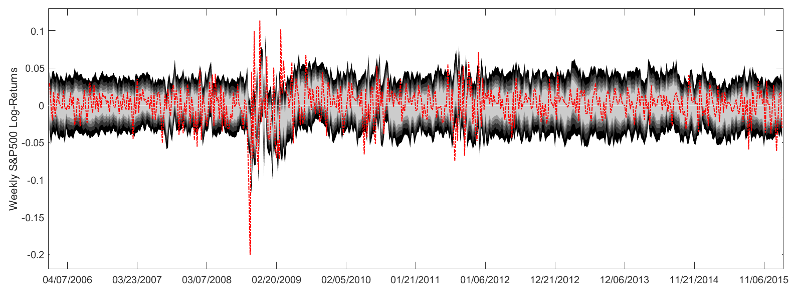
For the above settings, we receive the prediction intervals in Figure A1 for weekly S&P500 log-returns. To be precise, the light gray area reveals the 50%-prediction intervals, while the black areas specify the 90%-prediction intervals. Here, each new, slightly darker area corresponds to prediction levels increased by 10%. In addition, the red line shows the afterwards realized S&P500 log-returns. Please note that the prediction intervals cover the S&P500 returns quite well, as there is a moderate number of interval outliers. However, during the financial crisis in 2008/2009 we have a cluster of interval outliers, which calls for further analyses. Perhaps, the inclusion of regime-switching concepts may remedy this circumstance.
As supplement to Figure A1, 
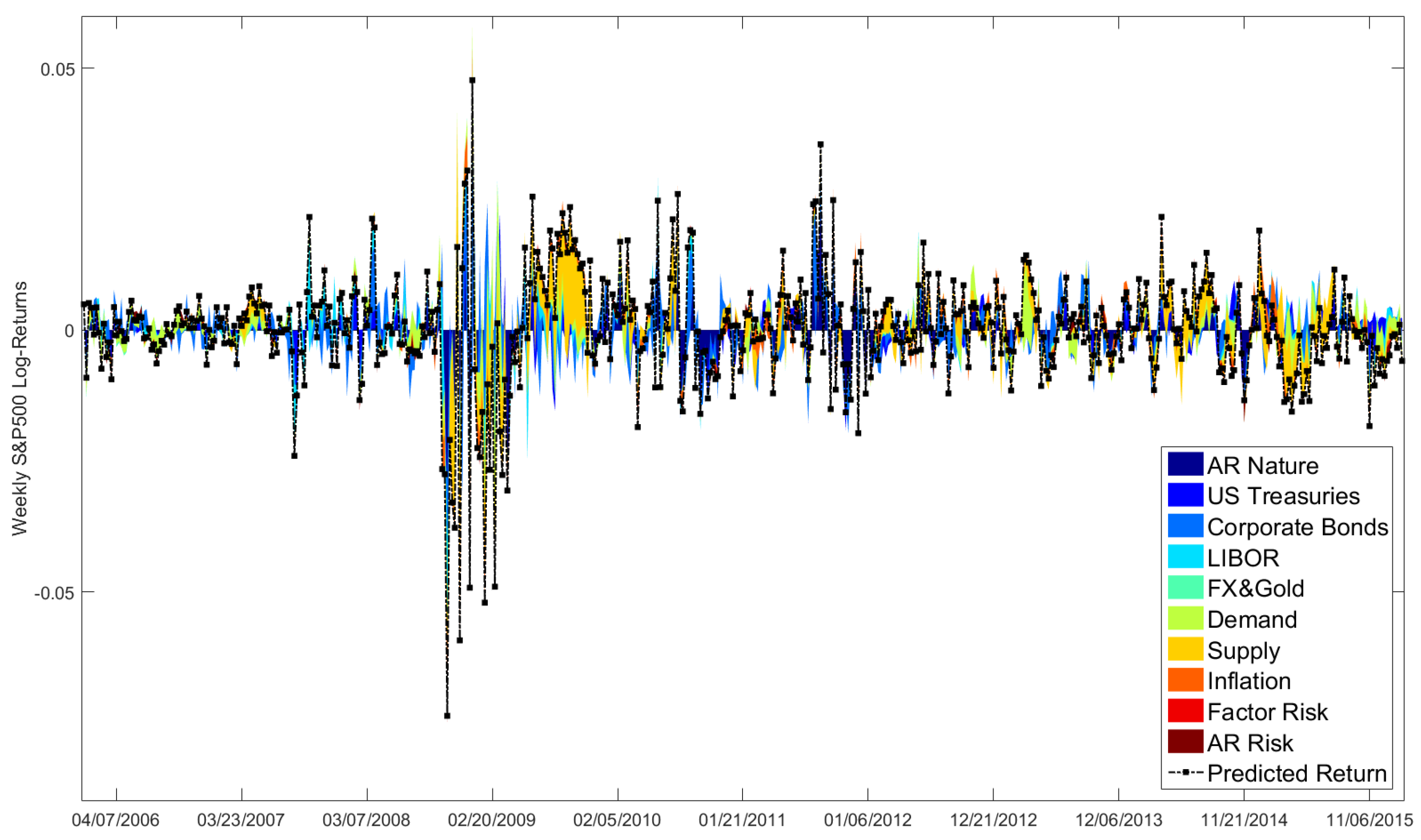
Figure A2 breaks the means of the predicted S&P500 log-returns down into the contributions of our panel data groups. In contrast to Figure A1, where Factor and AR Risks widened the prediction intervals, both do not matter in Figure A2. This makes sense, as we average the predicted returns, whose Factor and AR Risks are assumed to have zero mean. Dark and light blue colored areas detect how financial data affects our return predictions. In particular, during the financial crisis in 2008/2009 and in the years 2010–2012, when the United States (US) Federal Reserve intervened on capital markets in the form of its quantitative easing programs, financial aspects mainly drove our return predictions. Since the year 2012, the decomposition is more scattered and changes quite often, i.e., macroeconomic and financial events matter. 
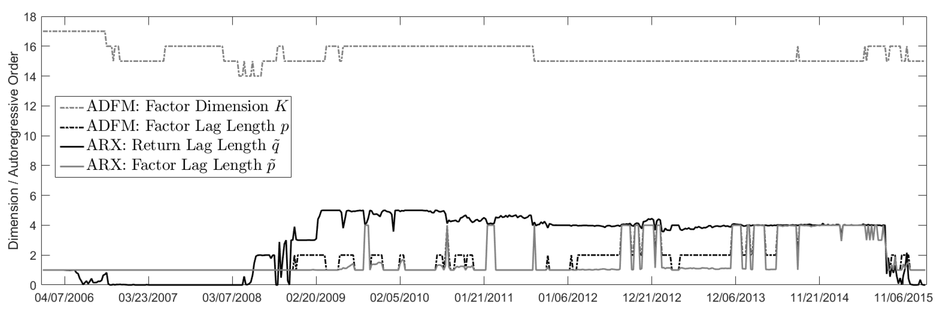
Figure A3 also supports the hypothesis that exogenous information increasingly affected the S&P500 returns in recent years. Although the factor dimension stayed within the range [15, 16] and we have for the autoregressive return order q ˜ = 4 , from mid-2013 until mid-2015 the factor lags p and p ˜ increased. This indicates a more complex ADFM and ARX modeling.
Next, we focus on the financial characteristics of the presented approach. Therefore, we verify whether the Trading Strategies (24) and (25) may benefit from the proper mapping of the prediction intervals. Here, we abbreviate Trading Strategy (24) based on the 50%-prediction intervals by Prediction Level PL 50, while (PL) 60 is its analog using the 60%-prediction intervals, etc. For simplicity, our cash account does not offer any interest rate, i.e., r ˜ t 0 for all times t 0 and transaction costs are neglected. In total, 
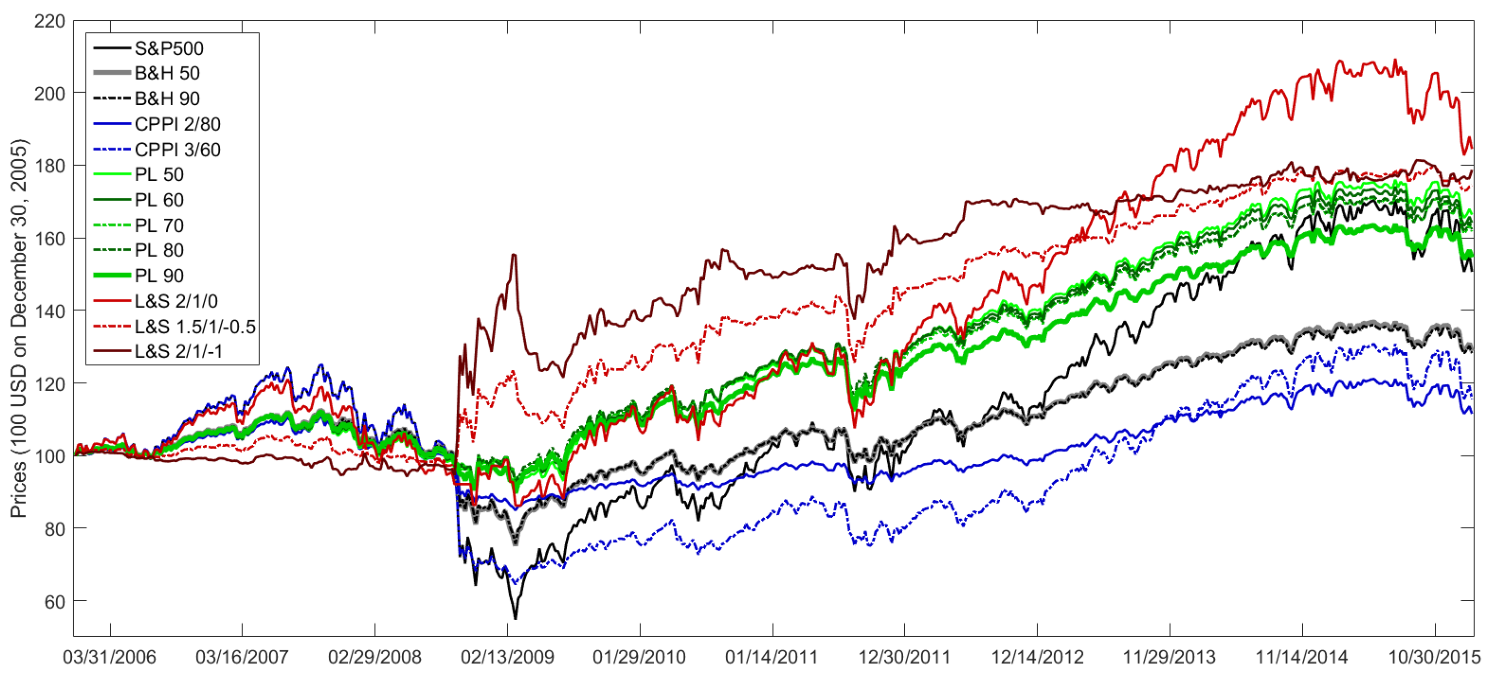
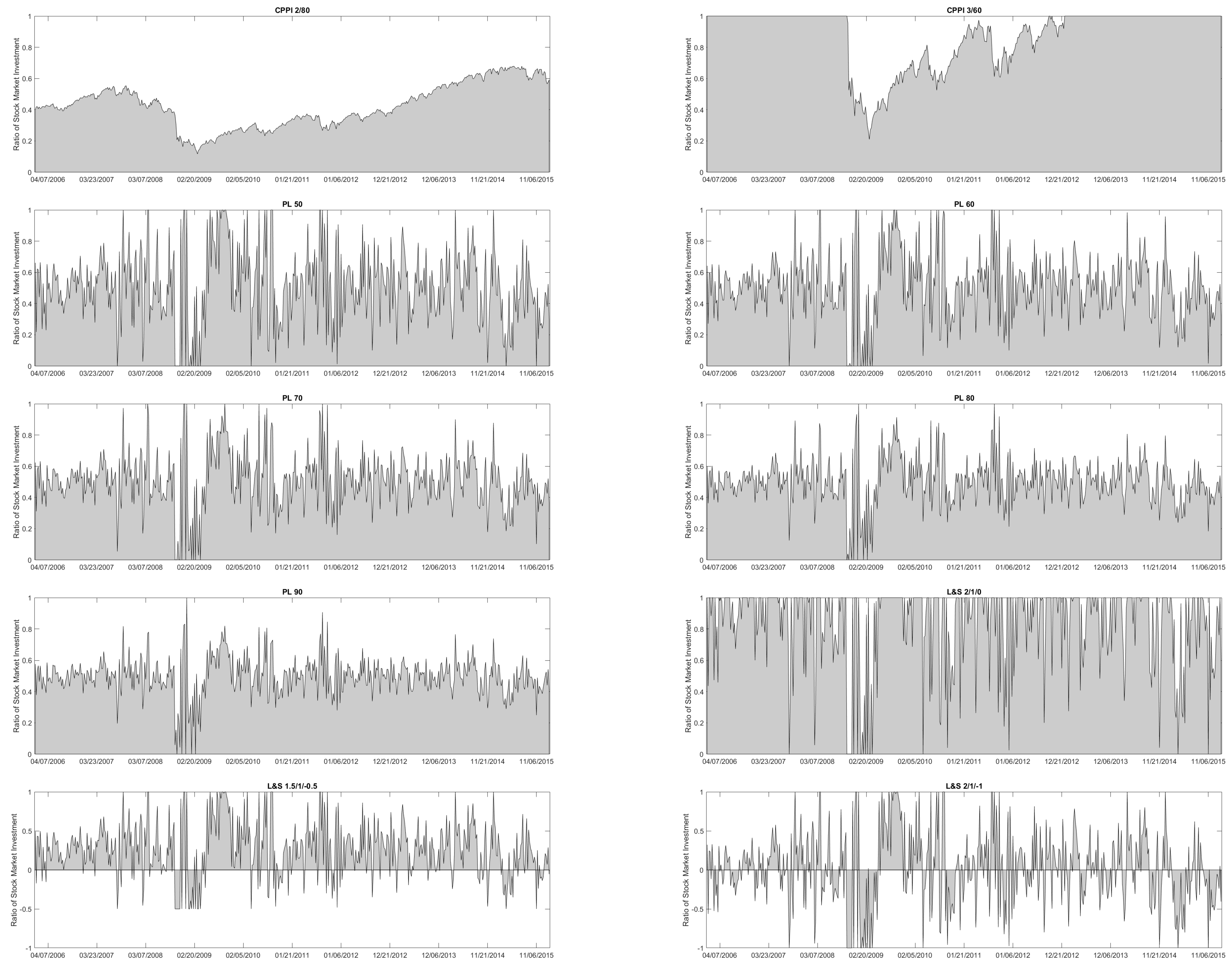
Figure A4 illustrates how an initial investment of 100 United States Dollar (USD) on December 30, 2005 in the trading strategies PL 50 until PL 90 with weekly rebalancing would have evolved. Hence, it shows a classical backtest.
In addition, we analyze how Leverage & Short Sales (L&S) change the risk-return profile of Trading Strategy (24). Again, we have for the cash account: r ˜ t 0 and there are zero transaction costs. That is, how the risk-return profile of Trading Strategy (25) deviates from the one in (24) and what the respective contribution of parameters α A , π U and π L is. In Figure A4, L&S 2/1/0 stands for Trading Strategy (25) with weekly rebalancing based on PL 50 with parameters α A = 2 , π U = 1 and π L = 0 . The trading strategy L&S 2/1/−1 is also based on PL 50, but has the parameters α A = 2 , π U = 1 and π L = 1 .
In Figure A4, the strategy S&P500 reveals how a pure investment in the S&P500 would have performed. Moreover, Figure A4 shows the price evolution of two Buy&Hold (B&H) and two Constant Proportion Portfolio Insurance (CPPI) strategies with weekly rebalancing. Hence, the Buy&Hold strategies serve as Constant Mix strategies. Here, B&H 50 denotes a Buy&Hold strategy with rebalanced S&P500 exposure on average of PL 50. Similarly, B&H 90 invests the averaged S&P500 exposure of PL 90. In Figure A4, CPPI 2/80 stands for a CPPI strategy with multiplier 2 and floor 80%. The floor of a CPPI strategy denotes the minimum repayment at maturity. For any point in time before maturity, the cushion represents the difference between the current portfolio value and the discounted floor. Here, discounting does not matter, since r ˜ t 0 t 0 holds. The multiplier of a CPPI strategy constitutes to what extent the positive cushion is leveraged. As long as the cushion is positive, the cushion times the multiplier, which is called exposure, is invested in the risky assets. Because of r ˜ t 0 t 0 , there is no penalty, if the exposure exceeds the current portfolio value. To avoid borrowing money, the portfolio value at a given rebalancing date caps the risky exposure in this section. As soon as the cushion is zero or becomes negative, the total wealth is deposited on the bank account with r ˜ t 0 for the remaining time to maturity. Further information about CPPI strategies is stated in, e.g., Black and Perold [45]. Similarly, CPPI 3/60 stands for a CPPI strategy with multiplier 3 and floor 60%.
Besides Figure A4, Table A10 lists some common performance and risk measures for all trading strategies. Then, we conclude: First, for higher prediction levels the Log-Return (Total, %) of its PL strategy decreases. E.g., compare PL 50 and PL 90. By definition, a high prediction level widens the intervals such that shifts in their location have less impact on the stock exposure π t in (24). As shown in Figure A5, all PL strategies are centered around a level of 50%, but PL 50 adjusts its stock exposure more often and to a bigger extent than PL 90. Second, all PL strategies have periods of time with a lasting stock exposure 50 % or 50 % . Over our out-of-sample period, PL 50 invests on average 51% of its wealth in the S&P 500, but it outperformed B&H 50 by far. Hence, changing our asset allocation by π t in (24) really paid off.
Except for the L&S strategies, PL 50 has the highest Log-Return (Total, %) and therefore, appears very attractive. However, the upside usually comes with a price. This is why we next focus on the volatilities of our trading strategies. In this regard, CPPI 2/80 offers with 0.93% the lowest weekly standard deviation. With its allocation in Figure A5 in mind, this makes sense, as CPPI 2/80 was much less exposed to the S&P500 than all others. Please note that Figure A5 also shows how CPPI 3/60 was hit by the financial crisis in 2007/2008, when its S&P500 exposure dramatically dropped from 100% on 3 October 2008 to 21% on 13 March 2009. For PL strategies, we get for the volatility an opposite picture compared to the Log-Return (Total, %), i.e., the higher the prediction level, the lower the weekly standard deviation is. This sounds reasonable, as PL 90 makes smaller bets than PL 50. For L&S strategies, Table A10 confirms that leveraging works as usual. Both, i.e., return and volatility, increased at the same time.
The Sharpe Ratio links the return and volatility of a trading strategy. Except for L&S 1.5/1/−0.5, the PL strategies offer the largest Sharpe Ratios. Therefore, PL 80 has the biggest weekly Sharpe Ratio of 7.39%. As supplement, Table A11 reveals that the Sharpe Ratios of PL 80 and PL 90 are significantly different to those of S&P500, CPPI 2/80 and CPPI 3/60. The differences within or between the PL and L&S strategies are not significant. The Omega Measure compares the upside and downside of a strategy. Based on Table A10, L&S 1.5/1/−0.5 and L&S 2/1/−1 have the largest Omega Measures given by 134.92% and 132.39%. The Omega Measures of the PL strategies lie in the range [121.34%, 124.94%], which are larger than those of the benchmark strategies in the range [103.86%, 111.16%]. The differences between all Omega Measures are not significant, see Table 4.16 in [41].
Similar to the volatility, CPPI 2/80 has the smallest 95% Value at Risk and 95% Conditional Value at Risk. The PL strategies have more or less the same weekly 95% VaR, since all lie in the range [ 1.99 % , 1.90 % ] . However, their 95% CVaR ranges from −3.19% to −2.78% and so, reflects that PL 50 makes bigger bets than PL 90. For L&S strategies, there is no pattern how leveraging and short selling affects the 95% VaR and CVaR. Finally, we consider the Maximum Drawdown based on the complete out-of-sample period. Please note that Figure A4 and Figure A5 and Table A10 confirm that CPPI 3/60 behaves like the S&P500, until it was knocked out by the financial crises in 2007/2008. This is why its Maximum Drawdown of −48.43% is close to the −56.24% of the S&P500. By contrast, the Maximum Drawdowns of the PL strategies lie in the range of [−19.91%, −17.37%], which is less than half. They are even smaller than the Maximum Drawdown of CPPI 2/80, which is −23.18%. For L&S strategies, short sales admit us to gain from a drop on the stock market, while leveraging boosts profits and losses. In total, this yields a scattered picture for their Maximum Drawdowns.
With the financial figures in mind, we recommend PL 50 for several reasons: First, it provides a decent return, which is steadily gained over the total period. Second, it has an acceptable volatility and a moderate downside. Please note that all PL strategies, L&S 1.5/1/−0.5 and L&S 2/1/−1 are positively skewed, which indicates a capped downside. The normalized histograms of the log-returns for all trading strategies can be found in Figure 4.6 from Ramsauer [41].
If we repeat the previous analysis for complete panel data, we can verify whether the inclusion of mixed-frequency information really pays off. Instead of all 33 time series in Appendix E, we restrict ourselves to US Treasuries, Corporate Bonds, London Interbank Offered Rate (LIBOR) and Foreign Exchange (FX)&Gold. Therefore, we have 22 time series without any missing observations. Again, we keep our rolling window of 364 weeks and gradually shift it over time, until we reach the sample end. For the upper limit of the factor dimension, we set K ¯ = 21 . At this stage, there are no obvious differences between the prediction intervals for incomplete and complete panel data [41] (Figure 4.7). If we break the means of the predicted log-returns in Figure A6 down into the contributions of the respective groups as shown in Figure A6, we have a different pattern than in Figure A2. E.g., Figure A2 detects supply as main driver at the turn of the year 2009/2010, whereas Figure A6 suggests US Treasuries and Corporate Bonds. However, in the years 2010–2012 US Treasuries gained in importance in Figure A6, which also indicates the interventions of the US Federal Reserve through its quantitative easing programs.
Next, we analyze the impact of the prediction intervals on Trading Strategies (24) and (25). Besides PL and L&S strategies of Figure A4 based on 33 variables, Figure A7 shows their analogs arising from 22 complete time series. Please note that the expression PL 50 (no) in Figure A7 is an abbreviation for PL 50 using panel data with no gaps. The same holds for L&S 2/1/0, etc. Besides the prices in Figure A7, Table A12 lists their performance and risk measures. The S&P exposure of the single strategies based on the 22 complete time series can be found in Figure 4.11 from Ramsauer [41]. Thus, we conclude: First, PL 50 (no) has a total log-return of 30.22%, which exceeds all other PL (no) strategies, but is much less than 50.93% of PL 50. Similarly, the L&S (no) strategies have a much lower log-return than their L&S counterparts. Second, PL 50 (no) changes its S&P500 exposure more often and to a larger extent than PL 90 (no). Third, the standard deviations of PL (no) strategies exceed their PL analogs such that their Sharpe Ratios are about half of the PL Sharpe Ratios. As shown in Table A13, the Sharpe Ratios of PL and PL (no) strategies are significantly different. Fourth, PL (no) strategies are dominated by their PL versions in terms of Omega Measure. Table 4.19 in [41] shows that such differences are not significant. Fifth, the 95% VaR and CVaR of the PL (no) strategies are slightly worse than of the PL alternatives, but their Maximum Drawdowns almost doubled in the absence of macroeconomic signals. Except for PL 50 (no), the returns of all PL (no) strategies, are negatively skewed [41] (Figure 4.12). This indicates that large profits were removed and big losses were added, respectively. All in all, we therefore suggest the inclusion of macroeconomic variables.
Eventually, we consider the Root-Mean-Square Error (RMSE) for weekly point forecasts of the S&P500 log-returns. We replace sampled factors and ARX coefficients by their estimates to predict the log-return of next week. In this context, an ARX based on incomplete panel data has a RMSE of 0.0272, while an ARX restricted to 22 variables provides a RMSE of 0.0292. Please note that a constant forecast r ^ t 0 yields a RMSE of 0.0259, the RMSEs of Autoregressive Models (ARs) with orders from 1–12 lie in the range 0.0260 , 0.0266 and the RMSEs of Random Walks with and without drift are 0.0380 and 0.0379, respectively. Therefore, our model is mediocre in terms of RMSE. Since the RMSE controls the size, but not the direction of the deviations, 
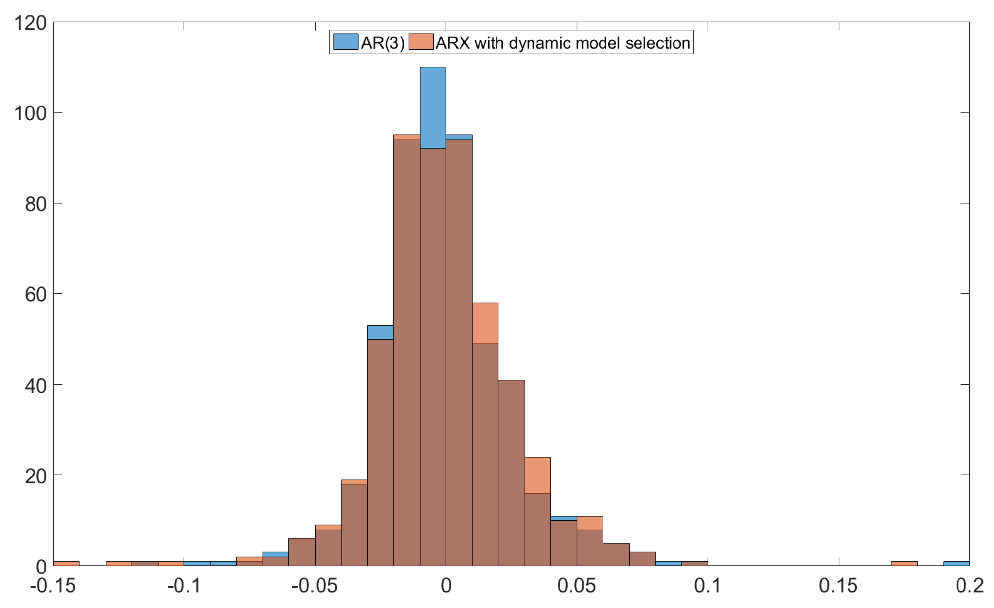
Figure A8 illustrates the deviations r ^ t r t of our ARX based on all panel data and the AR(3), which was best regarding RMSE. As Figure A8 shows, the orange histogram has 4 data points with r ^ t r t 0.10 . Our ARX predictions for 10/17/2008, 10/31/2008, 11/28/2008 and 03/13/2009 were too conservative, which deteriorated its RMSE. If we exclude these four dates, our mixed-frequency ARX has a RMSE of 0.0251, which beats all other models.
For comparing the predictive ability of competing forecasts, we perform a conditional Giacomini-White test. Our results rely on the MATLAB implementation available at http://www.execandshare.org/CompanionSite/site.do?siteId=116 (accessed on 13 December 2020) of the test introduced in Giacomini and White [46]. Furthermore, we consider the squared error loss function. We conclude: First, the inclusion of macroeconomic data in our approach is beneficial at a 10%-significance level. A comparison of our method based on incomplete panel data vs. complete financial data only provides a p-value of 0.06 and a test statistic of 5.61. In this context, forecasting with macroeconomic variables outperforms the forecasting relying on pure financial data by more than 50% of the time. Second, there are not any significant differences between our approach and an AR(3) or a constant forecast r ^ t 0 . By comparing our approach with an AR(3), we observe a p-value of 0.364. Similarly, we have a p-value of 0.355 compared to the constant forecast r ^ t 0 . Unfortunately, this also holds true, if we remove the four previously mentioned outliers from our prediction sample.
Finally, we verify the quality of our interval forecasts with respect to the Ratio of Interval Outliers (RIO) and Mean Interval Score (MIS) for prediction intervals in Table A14. For the respective definitions, we refer to Gneiting and Raftery [47], Brechmann and Czado [48] and Ramsauer [41]. In this context, the inclusion of mixed-frequency information provides some statistical improvements. Except for the 50%-prediction intervals, we have more outliers in Table A14, when the ARX relies on 22 complete time series than all 33 variables. Thus, the macroeconomic indicators make our model more cautious. Except for the 90%-prediction intervals based on complete panel data, all Ratios of Interval Outliers are below the aimed threshold. In contrast to RIO counting the number of interval outliers, MIS takes into account by how much the prediction intervals are exceeded. In this regard, the ARX using incomplete panel data dominates the ARX restricted to the 22 time series. All in all, this underpins again the advantages arising from the inclusion of macroeconomic information.

7. Conclusions and Final Remarks

We estimate ADFMs with homoscedastic, cross-sectionally correlated errors for incomplete panel data. Our approach alternately applies two EMs and selects the factor dimension and autoregressive order. The latter feature is important for empirical applications. Furthermore, estimated latent factors are used to model future dynamics of weekly S&P500 index returns in an autoregressive setting. In doing so, we are able to first quantify the contributions of the panel data to our point forecasts. Second, we construct prediction intervals for the weekly returns and define two dynamic trading strategies based on them. Our empirical application shows great potential of the proposed methodology for financial markets without short selling or leverage.
Our paper makes three contributions to the existing literature for incomplete panel data. First, it handles cross-sectionally correlated shocks usually ignored. Our MC simulation study shows that our approach outperforms the benchmark estimation of ADFMs in Bańbura and Modugno [20]. Second, our MLE does not link an EM and the KF/KS. We use instead the means and covariance matrices of the latent factors in closed form. Our MC simulation study reveals that MLE based on closed-form factor moments dominates MLE with the KF/KS. Third, we treat the stochastic factor dynamics in its general form and address the selection of the factor dimension as well as autoregressive order essential for practical applications.
The processing of the estimated factors is also novel. Instead of point estimates, we construct empirical prediction intervals for a return series. Besides exogenous information and autoregressive return characteristics, the prediction intervals incorporate uncertainties arising from the estimation of the factors and model parameters. Furthermore, we trace the means of our prediction intervals back to the original panel data and their high-frequency counterparts, respectively. This is an important feature for practitioners, as it offers them to compare our model-based output with their expectations. To gain information from the future index behavior, we propose two dynamic trading strategies. The first determines how much of the total wealth should be invested in the financial index depending on the prediction intervals. The second strategy shows how risk-return characteristics of the first can be adapted to the needs of an investor.
Our approach does not cover serially correlated errors. Therefore, future research could include the estimation of ADFMs with homoscedastic, serially and cross-sectionally correlated idiosyncratic errors for incomplete panel data. In a next step, an extension to heteroscedasticity or the incorporation of regime-switching concepts would be worthwhile. Finally, several ADFMs could be coupled by copulas to capture nonlinear inter-market dependencies similarly to Ivanov et al. [49].

Author Contributions

All authors substantially contributed to this article as follows: Conceptualization, all authors; Methodology, all authors; Software, F.R.; Validation, F.R. and A.M.; Formal Analysis, F.R.; Investigation, F.R.; Resources, all authors; Data Curation, F.R.; Writing—Original Draft Preparation, F.R. and A.M.; Writing—Review & Editing, F.R., A.M. and R.Z.; Visualization, F.R.; Supervision, M.D., F.S. and R.Z.; Project Administration, L.P., F.R. and A.M.; Funding Acquisition, M.D. and F.S. All authors have read and agreed to the published version of the manuscript.

Funding

The PhD position of Franz Ramsauer at Technical University of Munich was third-party funded by Pioneer Investments, which is now part of Amundi Asset Management. Otherwise, this research received no external funding.

Data Availability Statement

All underlying data is publicly available. The respective sources are stated in Appendix E in detail.

Acknowledgments

The authors want to thank the editor and two anonymous reviewers for their very helpful suggestions, which essentially contributed to an improved manuscript. Franz Ramsauer gratefully acknowledges the support of Pioneer Investments, which is now part of Amundi Asset Management, during his doctoral phase.

Conflicts of Interest

The authors declare no conflict of interest. The sponsorship had no impact on the design of the study, in the collection, analyses, and interpretation of data, in the writing of the manuscript, nor in the decision to publish the results.

Appendix A. Algorithms

Algorithm A1: Estimate ADFMs based on complete panel data
Forecasting 03 00005 i001
Algorithm A2: Estimate ADFMs based on incomplete panel data
Forecasting 03 00005 i002

Appendix B. Simulation Results

Table A1. Means of trace R 2 for random ADFMs using standard KF and KS.
Stock  a Stock/Flow (Average)  b Stock/Change in Flow (Average)  c
Ratio of Missing DataRatio of Missing DataRatio of Missing Data
N T 0%10%25%40%0%10%25%40%0%10%25%40%
K = 1 , p = 1
251000.940.930.930.910.940.930.920.860.940.930.920.87
255000.980.980.970.960.980.970.970.940.980.970.970.95
501000.950.940.940.910.940.940.920.840.950.940.930.86
505000.980.980.980.980.980.980.980.960.980.980.980.96
751000.950.950.920.830.950.940.890.890.950.940.88NaN
755000.990.990.980.980.990.980.980.960.990.980.980.97
Ratio of Missing DataRatio of Missing DataRatio of Missing Data
N T 0%10%25%40%0%10%25%40%0%10%25%40%
K = 3 , p = 2
251000.880.870.850.800.880.870.840.760.880.870.830.75
255000.970.960.960.940.970.960.940.870.970.950.940.88
501000.900.900.880.850.900.890.860.770.900.890.850.77
505000.980.980.970.960.980.970.970.910.980.970.960.92
751000.910.900.880.840.900.890.85NaN0.910.890.850.75
755000.980.980.980.970.980.980.970.930.980.970.970.94
K = 5 , p = 2
251000.880.870.840.790.880.870.820.750.880.860.820.75
255000.970.960.950.920.970.960.930.850.970.950.930.85
501000.890.890.870.840.890.880.850.780.890.880.840.77
505000.970.970.970.960.970.970.960.890.970.960.950.90
751000.900.890.870.850.890.880.850.780.900.880.850.78
755000.980.980.980.970.980.980.970.910.980.970.970.92
a : For incomplete time series a stock variable is assumed. b : For incomplete data, N / 2 and N / 2 time series are stock and flow (average formulation) variables, respectively. c : For incomplete data, N / 2 and N / 2 time series serve as stock or change in flow (average formulation) variables.
Table A2. Means of trace R 2 for random ADFMs using closed-form factor moments.
Stock  a Stock/Flow (Average)  b Stock/Change in Flow (Average)  c
Ratio of Missing DataRatio of Missing DataRatio of Missing Data
N T 0%10%25%40%0%10%25%40%0%10%25%40%
K = 1 , p = 1
251000.960.950.950.950.960.950.950.920.960.950.940.92
255000.980.980.970.970.980.980.970.950.980.970.970.95
501000.960.960.960.950.960.960.950.940.960.950.960.94
505000.990.990.980.980.990.980.980.970.990.980.980.97
751000.960.960.960.960.960.960.960.940.970.960.960.94
755000.990.990.990.990.990.990.990.970.990.980.990.98
K = 3 , p = 2
251000.950.950.940.930.950.940.940.900.950.940.940.90
255000.980.970.970.960.980.970.960.930.980.960.960.94
501000.960.950.950.950.960.950.950.930.960.950.950.93
505000.990.980.980.980.990.980.980.960.990.980.980.96
751000.960.960.960.960.960.960.960.940.960.950.960.94
755000.990.990.990.980.990.990.980.960.990.980.980.97
K = 5 , p = 2
251000.950.940.940.930.950.940.930.890.950.930.930.88
255000.980.970.970.950.980.970.960.920.980.960.960.92
501000.960.960.950.950.960.950.950.930.960.950.950.93
505000.990.980.980.980.990.980.980.950.990.980.980.96
751000.960.960.960.960.960.950.960.940.960.950.960.94
755000.990.990.990.980.990.980.980.960.990.980.980.97
All displayed means are derived from 500 MC simulations for known dimensions K and p. a : For incomplete time series a stock variable is assumed. b : For incomplete data, N / 2 and N / 2 time series are stock and flow (average formulation) variables, respectively. c : For incomplete data, N / 2 and N / 2 time series serve as stock or change in flow (average formulation) variables.
Table A3. Ratios of trace R 2 means for random ADFMs using both approaches.
Stock  a Stock/Flow (Average)  b Stock/Change in Flow (Average)  c
Ratio of Missing DataRatio of Missing DataRatio of Missing Data
N T 0%10%25%40%0%10%25%40%0%10%25%40%
K = 1 , p = 1
251001.021.021.021.041.021.021.031.081.021.021.031.06
255001.001.001.001.001.001.001.001.011.001.001.001.01
501001.021.021.021.051.021.021.031.131.021.021.031.09
505001.001.001.001.001.001.001.001.011.001.001.001.01
751001.011.021.041.151.011.021.081.071.011.021.09NaN
755001.001.001.001.001.001.001.001.011.001.001.001.00
K = 3 , p = 2
251001.081.081.111.161.081.081.121.191.081.081.131.20
255001.011.011.021.021.011.011.021.071.011.011.021.07
501001.061.071.081.131.061.071.111.211.061.071.121.21
505001.011.011.011.021.011.011.021.051.011.011.021.05
751001.061.071.091.141.061.071.12NaN1.061.071.131.24
755001.011.011.011.011.011.011.011.041.011.011.011.03
K = 5 , p = 2
251001.081.081.121.181.081.081.131.181.081.081.141.18
255001.011.011.021.031.011.011.031.081.011.011.031.09
501001.081.081.091.131.081.081.121.191.081.081.131.20
505001.011.011.011.021.011.011.021.071.011.011.031.07
751001.071.081.101.131.071.081.121.201.071.081.131.21
755001.011.011.011.021.011.011.021.051.011.011.021.05
The displayed ratios are derived from 500 MC simulations for known dimensions K and p. In doing so, each figure represents the mean of the trace R 2 in Table A2 divided by its counterpart in Table A1. a : For incomplete time series a stock variable is assumed. b : For incomplete data, N / 2 and N / 2 time series are stock and flow (average formulation) variables, respectively. c : For incomplete data, N / 2 and N / 2 time series serve as stock or change in flow (average formulation) variables.
Table A4. Comparison of trace R 2 means for random ADFMs using the approach of [20] and our two-step estimation method.
BM  a CFM b CFM/BM
Ratio of Missing DataRatio of Missing DataRatio of Missing Data
N T 0%10%25%40%0%10%25%40%0%10%25%40%
K = 3 , p = 2
251000.930.930.920.910.950.950.940.931.021.021.021.02
255000.970.970.970.960.980.970.970.961.001.001.001.00
501000.940.940.930.930.960.960.950.951.021.021.021.02
505000.980.980.980.980.990.980.980.981.001.001.001.00
751000.940.940.940.940.960.960.960.961.021.021.021.02
755000.980.980.980.980.990.990.990.981.001.001.001.00
K = 5 , p = 4
251000.900.900.880.850.940.940.930.921.051.051.061.08
255000.970.960.960.940.970.970.960.951.011.011.011.01
501000.910.910.910.900.960.950.950.951.051.051.051.05
505000.980.980.970.970.980.980.980.981.011.011.011.01
751000.920.920.910.910.960.960.960.951.051.051.051.05
755000.980.980.980.970.990.990.990.981.011.011.011.01
K = 7 , p = 3
251000.910.910.880.830.950.940.930.911.041.041.051.09
255000.970.960.950.940.970.970.960.941.011.011.011.01
501000.920.920.920.910.960.950.950.951.031.031.041.04
505000.980.980.970.970.980.980.980.981.011.011.011.01
751000.930.930.930.920.960.960.960.951.031.031.031.04
755000.980.980.980.980.990.990.990.981.011.011.011.01
The means in columns BM and CFM are derived from 500 MC simulations for known dimensions K and p. The ratios in column CFM/BM denote the means in column CFM divided by their counterparts in column BM. In case of incomplete data, all time series are supposed to be stock variables. a : Abbreviation for the estimation method in [20]. b : Abbreviation for closed-form factor moments.
Table A5. Means of trace R 2 for random ADFMs of low dimensions using our two-step estimation method with m = 1 .
Trace R 2 Estimated KEstimated p
Ratio of Missing DataRatio of Missing DataRatio of Missing Data
N T 0%10%25%40%0%10%25%40%0%10%25%40%
K = 3 , p = 2
251000.950.940.920.872.992.982.892.721.651.741.691.76
255000.980.970.970.943.003.002.992.932.042.042.052.04
501000.960.960.960.943.003.003.002.951.721.781.721.70
505000.990.980.980.983.003.003.003.002.032.032.062.06
751000.960.960.960.963.003.003.003.001.681.711.761.78
755000.990.990.990.983.003.003.003.002.052.052.052.06
K = 5 , p = 1
251000.780.740.680.603.743.503.162.741.011.031.051.04
255000.850.830.770.684.174.083.753.321.001.011.021.06
501000.920.890.830.744.624.393.953.441.011.011.021.04
505000.980.980.960.914.994.974.854.521.001.001.011.01
751000.960.940.890.824.934.754.363.871.011.011.011.02
755000.990.990.990.985.005.005.004.961.011.001.011.00
K = 5 , p = 2
251000.770.720.640.563.783.453.052.641.601.621.721.80
255000.850.810.740.644.234.063.673.212.002.012.012.01
501000.920.880.790.704.704.363.823.291.471.561.661.79
505000.980.980.960.894.994.984.834.452.012.002.002.00
751000.950.940.870.794.944.834.283.731.441.481.591.71
755000.990.990.990.985.005.005.004.972.012.002.002.00
Table A6. Means of trace R 2 for random ADFMs of low dimensions using our two-step estimation method with m = 1 2 .
Trace R 2 Estimated KEstimated p
Ratio of Missing DataRatio of Missing DataRatio of Missing Data
N T 0%10%25%40%0%10%25%40%0%10%25%40%
K = 3 , p = 2
251000.950.950.940.933.003.003.003.011.671.671.631.65
255000.980.980.970.963.003.003.003.022.052.032.032.04
501000.960.950.960.953.003.003.003.011.721.751.771.76
505000.990.980.980.983.003.003.003.022.032.042.062.04
751000.960.960.960.963.003.003.003.001.701.721.761.73
755000.990.990.990.983.003.003.003.022.032.042.042.05
K = 5 , p = 1
251000.940.920.900.874.874.754.654.501.011.011.011.01
255000.970.970.960.944.964.974.924.851.001.001.001.01
501000.960.960.950.955.005.004.984.911.001.011.011.01
505000.990.990.980.985.005.005.005.001.001.001.011.00
751000.960.960.960.965.005.005.004.991.001.001.011.01
755000.990.990.990.995.005.005.005.001.001.001.001.00
K = 5 , p = 2
251000.940.920.890.854.884.784.604.471.351.421.431.47
255000.970.970.950.934.984.964.924.852.002.002.002.00
501000.960.960.950.945.005.004.984.921.451.461.431.47
505000.990.980.980.985.005.005.005.002.002.012.002.00
751000.960.960.960.965.005.005.004.991.461.421.421.41
755000.990.990.990.985.005.005.005.002.002.002.002.01
All means in column trace R 2 are derived from 500 MC simulations for unknown dimensions K and p. Therefore, columns two and three show the corresponding means of the estimated factor dimension K and lag length p. In case of incomplete data, all time series are supposed to be stock variables.
Table A7. Means of trace R 2 for random ADFMs of large dimensions using our two-step estimation method with m = 1 2 .
Trace R 2 Estimated KEstimated p
Ratio of Missing DataRatio of Missing DataRatio of Missing Data
N T 0%10%25%40%0%10%25%40%0%10%25%40%
K = 17 , p = 1
303000.750.740.720.6712.0012.0012.0012.001.001.001.001.00
304000.740.730.710.6712.0012.0012.0012.001.001.001.001.00
353000.750.750.730.6912.0012.0012.0012.001.001.001.001.00
354000.750.740.720.6912.0012.0012.0012.001.001.001.001.00
403000.760.750.740.7112.0012.0012.0012.001.001.001.001.00
404000.750.750.730.7012.0012.0012.0012.001.001.001.001.00
K = 17 , p = 2
303000.740.730.700.6612.0012.0012.0012.001.801.781.811.77
304000.730.720.700.6512.0012.0012.0012.001.981.981.991.98
353000.740.730.710.6812.0012.0012.0012.001.881.831.841.83
354000.740.730.710.6712.0012.0012.0012.002.002.002.001.99
403000.750.740.720.6912.0012.0012.0012.001.891.871.881.89
404000.740.730.720.6912.0012.0012.0012.002.002.001.991.99
Table A8. Means of trace R 2 for random ADFMs of large dimensions using our two-step estimation method with m = 1 33 .
Trace R 2 Estimated KEstimated p
Ratio of Missing DataRatio of Missing DataRatio of Missing Data
N T 0%10%25%40%0%10%25%40%0%10%25%40%
K = 17 , p = 1
303000.960.950.930.8216.9216.8816.9218.741.001.001.001.00
304000.970.960.930.8316.9416.9116.9218.191.001.001.001.00
353000.970.970.950.8916.9916.9916.9917.801.001.001.001.00
354000.980.970.950.8916.9916.9917.0017.681.001.001.001.00
403000.980.970.960.9117.0017.0017.0018.001.001.001.001.00
404000.980.980.970.9217.0017.0017.0017.621.001.001.001.00
K = 17 , p = 2
303000.960.950.910.7916.9216.9216.9519.851.401.411.311.03
304000.960.950.920.8016.9516.9516.9419.191.911.891.871.32
353000.970.960.950.8716.9917.0017.0018.371.451.461.461.21
354000.970.970.950.8817.0017.0017.0117.991.951.931.911.64
403000.970.970.960.9117.0017.0017.0117.951.531.551.511.37
404000.980.970.960.9117.0017.0017.0018.081.941.951.941.65
Table A9. Means of trace R 2 for random ADFMs of large dimensions using our two-step estimation method with m = 1 66 .
Trace R 2 Estimated KEstimated p
Ratio of Missing DataRatio of Missing DataRatio of Missing Data
N T 0%10%25%40%0%10%25%40%0%10%25%40%
K = 17 , p = 1
303000.970.960.920.8017.0017.0017.6621.901.001.001.001.00
304000.970.960.920.8117.0017.0017.4821.841.001.001.001.00
353000.970.970.950.8717.0017.0017.3921.951.001.001.001.00
354000.980.970.950.8817.0017.0017.2021.811.001.001.001.00
403000.980.970.960.9217.0017.0017.2021.391.001.001.001.00
404000.980.980.960.9317.0017.0017.1120.181.001.001.001.00
K = 17 , p = 2
303000.960.950.900.7817.0017.0018.3221.971.411.391.181.00
304000.970.960.910.7917.0017.0017.9521.971.921.881.591.02
353000.970.960.940.8517.0017.0017.9822.001.491.481.290.99
354000.970.970.950.8617.0017.0017.3821.991.921.931.851.06
403000.970.970.960.9117.0017.0117.4721.951.541.541.440.95
404000.980.970.960.9217.0017.0117.2121.661.961.961.911.16
The means in column trace R 2 are derived from 500 MC simulations for unknown dimensions K and p. Therefore, columns two and three show the corresponding means of the estimated factor dimension K and lag length p. In case of incomplete data, all time series are supposed to be stock variables.

Appendix C. Empirical Results—Illustrations

Figure A1. Prediction intervals for S&P500 log-returns of the subsequent week (gray and black areas) and afterwards realized S&P500 log-returns (red line). The light gray area reveals the 50%-prediction intervals, whereas the black areas define the 90%-prediction intervals. Here, the prediction level gradually increases by 10% for each new, slightly darker area.
Forecasting 03 00005 g0a1
Figure A2. Decomposition of the S&P500 log-returns predicted for the next week.
Forecasting 03 00005 g0a2
Figure A3. Dimensions and lag orders of factors or returns of the predicted S&P500 log-returns.
Forecasting 03 00005 g0a3
Figure A4. Evolution of an initial investment of 100 USD in diverse single-market strategies (S&P500, B&H, CPPI, PL and L&S) over the out-of-sample period from December 30, 2005 until February 5, 2016. All strategies are weekly rebalanced and have zero transaction costs.
Forecasting 03 00005 g0a4
Figure A5. Percentage of total wealth invested in the S&P500 for diverse single-market trading strategies (CPPI, PL and L&S) over the out-of-sample period from 30 December 2005 until 5 February 2016.
Forecasting 03 00005 g0a5
Figure A6. Decomposition of S&P500 log-returns predicted for next week, when the panel data is restricted to complete time series.
Forecasting 03 00005 g0a6
Figure A7. Evolution of an initial investment of 100 USD in PL and L&S strategies based on complete and incomplete panel data over the out-of-sample period from December 30, 2005 until February 5, 2016. All strategies are weekly rebalanced and have zero transaction costs.
Forecasting 03 00005 g0a7
Figure A8. Differences between point forecasts and realizations of weekly S&P500 log-returns. The blue histogram shows such differences, when the return predictions arise from an AR(3). The orange histogram uses forecasts of our ARX based on mixed-frequency panel data.
Forecasting 03 00005 g0a8

Appendix D. Empirical Results—Tables

Table A10. Comparison of trading strategies for the out-of-sample period from 30 December 2005 until 5 February 2016.
S&P500B&HCPPIPrediction LevelLeverage & Short Sales
50902/803/6050607080902/1/01.5/1/−0.52/1/−1
Log-Return (Total, %)40.9525.3024.8410.8714.4550.9349.5548.1248.4743.5761.2355.5958.08
Log-Return (Wkly., %)  a 0.080.050.050.020.030.100.090.090.090.080.120.110.11
Std. Dev. (Wkly., %)  b 2.591.311.290.932.041.371.321.281.251.221.971.321.76
Sharpe Ratio (Wkly., %) c :3.003.653.672.221.347.057.127.117.396.785.897.976.26
Omega Measure (Wkly., %) d 109.08111.12111.16106.24103.86124.94124.37123.70124.03121.34118.51134.92132.39
95% VaR (Wkly., %) e−4.39−2.22−2.17−1.53−3.37−1.99−1.92−1.90−1.95−1.92−3.41−1.59−1.67
95% CVaR (Wkly., %) f −6.50−3.25−3.18−2.45−5.20−3.19−3.07−2.97−2.84−2.78−4.87−2.85−3.46
Max. Drawdown (in %) g −56.24−33.12−32.50−23.18−48.43−18.61−17.63−17.37−17.84−19.91−28.71−12.90−21.87
For each criterion, the bold value highlights the overall best strategy, whereas the bold and underlined value emphasizes the best strategy without Leverage & Short Sales (L&S). a : The considered period of time consists of 527 weeks. Therefore, it holds: Log Return ( Wkly . ) = Log Return ( Total ) / 527 . b : As standard deviation the square root of the empirical variance, i.e., the squared deviation from the Log−Return (Wkly.) divided by 526, is used. c : The Sharpe Ratio divides the expected excess return by its standard deviation. As the cash account does not provide any yield, the return of the benchmark is zero. d : The Omega Measure divides the upside by the downside of the expected excess returns, i.e., it is the ratio of the averaged positive and negative parts of Log−Return (Wkly.). e: For a fixed time horizon and confidence level α , the Value at Risk reflects the maximal Log−Return (Wkly.) that is not exceeded with probability 1 α . Mathematically, this means: 95% VaR (Wkly.) = sup r | P Log Return ( Wkly . ) < r 0.05 . f : For a fixed time horizon and confidence level α , the Conditional Value at Risk or Expected Shortfall is the expected return given that Log−Return (Wkly.) is below the α VaR, i.e., 95% CVaR (Wkly.) = E Log Return ( Wkly . ) | Log Return ( Wkly . ) . g : The Maximum Drawdown reveals the lowest discrete return, i.e., the highest loss to be gained during the complete out-of-sample period.
Table A11. Test statistic of Jobson and Korkie [50] for Sharpe Ratios.
S&P500B&HCPPIPrediction LevelLeverage & Short Sales
50902/803/6050607080902/1/01.5/1/−0.52/1/−1
S&P500x4.66114.66340.43291.11201.30561.37961.43931.67561.74591.03330.89080.4720
B&H 50xx4.76990.79311.48061.11931.18821.24191.47081.49890.81710.78540.3820
B&H 90xxx0.80121.48851.11491.18371.23721.46591.49300.81200.78290.3799
CPPI 2/80xxxx0.80321.51771.60871.67031.87721.87281.36771.06580.6031
CPPI 3/60xxxxx1.60941.67921.72371.89741.95831.44951.12540.6900
PL 50xxxxxx0.23150.10250.38350.22051.02670.34330.1782
PL 60xxxxxxx0.04410.40520.32561.20360.29790.1878
PL 70xxxxxxxx0.68220.38461.25590.28300.1784
PL 80xxxxxxxxx1.15681.53090.17540.2242
PL 90xxxxxxxxxx0.77850.31880.0976
L&S 2/1/0xxxxxxxxxxx0.62830.0751
L&S 1.5/1/-0.5xxxxxxxxxxxx0.8438
L&S 2/1/-1xxxxxxxxxxxxx
Values marked in dark gray are significant for level 5% (test statistic: 1.96), while light gray ones are significant for level 10% (test statistic: 1.64).
Table A12. Comparison of trading strategies for the out-of-sample period from 30 December 2005 until 5 February 2016.
Prediction Level (no)Leverage & Short Sales (no)
50607080902/1/01.5/1/ 0 . 5 2/1/ 1
Log-Return (Total, %)30.2221.9222.1220.3518.6247.9223.1116.50
Log-Return (Wkly., %) a 0.060.040.040.040.040.090.040.0300
Std. Dev. (Wkly., %) b 1.531.491.441.411.382.101.351.57
Sharpe Ratio (Wkly., %) c 3.752.802.912.742.564.333.242.00
Omega Measure (Wkly., %) d 112.79109.18109.34108.66107.97113.33112.67108.28
95% VaR (Wkly., %) e−2.18−2.06−1.99−2.03−2.15−3.21−1.73−2.05
95% CVaR (Wkly., %) f −3.88−3.85−3.70−3.56−3.47−5.17−3.52−3.97
Max. Drawdown (in %) g −30.75−33.67−34.56−35.13−35.82−42.34−27.24−34.12
For each criterion, the bold value highlights the overall best strategy, whereas the bold and underlined value emphasizes the best strategy without Leverage & Short Sales (L&S). a : The considered period of time consists of 527 weeks. Therefore, it holds: Log Return ( Wkly . ) = Log Return ( Total ) / 527 . b : As standard deviation the square root of the empirical variance, i.e., the squared deviation from the Log−Return (Wkly.) divided by 526, is used. c : The Sharpe Ratio divides the expected excess return by its standard deviation. As the cash account does not provide any yield, the return of the benchmark is zero. d : The Omega Measure divides the upside by the downside of the expected excess returns, i.e., it is the ratio of the averaged positive and negative parts of Log−Return (Wkly.). e: For a fixed time horizon and confidence level α , the Value at Risk reflects the maximal Log−Return (Wkly.) that is not exceeded with probability 1 α . Mathematically, this means: 95% VaR (Wkly.) = sup r | P Log Return ( Wkly . ) < r 0.05 . f : For a fixed time horizon and confidence level α , the Conditional Value at Risk or Expected Shortfall is the expected return given that Log−Return (Wkly.) is below the α VaR, i.e., 95% CVaR (Wkly.) = E Log Return ( Wkly . ) | Log Return ( Wkly . ) . g : The Maximum Drawdown reveals the lowest discrete return, i.e, the highest loss to be gained during the complete out-of-sample period.
Table A13. Test statistic of Jobson and Korkie [50] for Sharpe Ratios
Prediction LevelLeverage & Short SalesPrediction Level (no)Leverage & Short Sales (no)
50607080902/1/01.5/1/−0.52/1/−150607080902/1/01.5/1/−0.52/1/−1
PL 50x0.23150.10250.38350.22051.02670.34330.17821.52611.81441.71311.71621.72331.19951.21131.1017
PL 60xx0.04410.40520.32561.20360.29790.18781.61771.92471.82281.82641.83221.28911.22351.1001
PL 70xxx0.68220.38461.25590.28300.17841.67052.00731.91121.92091.92861.35351.20351.0779
PL 80xxxx1.15681.53090.17540.22421.90302.29252.21702.24192.25091.64641.25261.1023
PL 90xxxxx0.77850.31880.09761.69102.24672.23252.31262.36331.57311.02520.9401
L&S 2/1/0xxxxxx0.62830.07511.02061.39531.32941.37031.40970.78760.79890.8041
L&S 1.5/1/-0.5xxxxxxx0.84381.00641.13601.07581.07481.07960.79951.33681.6229
L&S 2/1/-1xxxxxxxx0.44390.57710.54610.55900.57530.32160.66351.1484
PL (no) 50xxxxxxxxx1.56430.99870.92680.90270.47720.23340.4231
PL (no) 60xxxxxxxxxx0.33280.09330.27631.36980.16650.1762
PL (no) 70xxxxxxxxxxx0.51490.59161.33640.11520.1903
PL (no) 80xxxxxxxxxxxx0.60661.44780.15780.1495
PL (no) 90xxxxxxxxxxxxx1.54530.20080.1087
L&S (no) 2/1/0xxxxxxxxxxxxxx0.34850.4753
L&S (no) 1.5/1/-0.5xxxxxxxxxxxxxxx0.5895
L&S (no) 2/1/-1xxxxxxxxxxxxxxxx
Values marked in dark gray are significant for level 5% (test statistic: 1.96), while light gray ones are significant for level 10% (test statistic: 1.64).
Table A14. Comparison of RIO and MIS for weekly S&P500 log-returns based on the out-of-sample period from 30 December 2005 until 5 February 2016.
MeasurePanel DataPrediction Level
50%60%70%80%90%
RIOincomplete0.44020.33970.25240.15940.0930
RIOcomplete0.42690.35480.26380.17650.1139
MISincomplete0.06350.07130.08160.09630.1240
MIScomplete0.06630.07490.08540.10100.1303
Bold figures highlight the best value of each category, i.e., for the n-prediction interval in rows 1–2 the RIO closest to (1 − v) and in rows 3–4 the lowest MIS are marked in bold.

Appendix E. Underlying Data

Table A15 describes the panel data considered. For clarity reasons, we distinguish between the following categories: real output and income; employment and hours; consumption; housing starts and sales; real inventories, orders, and unfilled orders; stock prices; foreign exchange rates; interest rates; money and credit quantity aggregates; price indices; average hourly earnings; miscellaneous; mixed-frequency time series; observed variables Y t .
The total sample ranges from 8 January 1999 to 5 February 2016 and is updated weekly. However, it comprises monthly and quarterly time series marked by “m” or “q” in the column Freq. as well as shorter time series as indicated in the column Time span. E.g., see time series MBST with its first observation in December 2002. For our empirical study we prepare vintage data by taking publication delays into account. For instance, for GDP data we assume a publication delay of 140 days, i.e., we include the Q3/2015 GDP figures on 19 February 2016 representing the first Friday after the assumed publication delay of 140 days based on 1 October 2015 which denotes the end of Q3/2015. For our underlying vintage data incl. the assumed publication delays please see our provided supplementary data.
For assumed data types, we have in column Type: stock (1), sum formulation of flow variable (2), average version of flow variable (3), sum formulation of change in flow variable (4) and average version of change in flow variable (5). Please note that for complete time series the data type does not matter, since all yield an identity matrix for matrix Q i .
Regarding data transformations in the scope of the preprocessing phase the column Trans. distinguishes between: no transformation (1), first difference (2), second difference (3), logarithm (4) and first difference of logarithm (5). This classification is in accordance with Bernanke et al. [51]. The column Series description provides information on how publication delays are taken into account and highlights seasonality adjustments: Seasonally Adjusted (SA) and Not Seasonally Adjusted (NSA).
Table A15. Panel data description.
No.Series IDTime SpanFreq.TypeTrans.Series Description
US Treasuries
1.DGS3MO1999/01/08–2016/02/05d123-Month Treasury Constant Maturity Rate, percent, NSA, delay of 1 day, https://research.stlouisfed.org/fred2/series/DGS3MO (accessed on 13 December 2020)
2.DTB31999/01/08–2016/02/05d123-Month Treasury Bill: Secondary Market Rate, percent, NSA, delay of 1 day, https://research.stlouisfed.org/fred2/series/DTB3 (accessed on 13 December 2020)
3.DGS11999/01/08–2016/02/05d121-Year Treasury Constant Maturity Rate, percent, NSA, delay of 1 day, https://research.stlouisfed.org/fred2/series/DGS1 (accessed on 13 December 2020)
4.DGS21999/01/08–2016/02/05d122-Year Treasury Constant Maturity Rate, percent, NSA, delay of 1 day, https://research.stlouisfed.org/fred2/series/DGS2 (accessed on 13 December 2020)
5.DGS31999/01/08–2016/02/05d123-Year Treasury Constant Maturity Rate, percent, NSA, delay of 1 day, https://research.stlouisfed.org/fred2/series/DGS3 (accessed on 13 December 2020)
6.DGS51999/01/08–2016/02/05d125-Year Treasury Constant Maturity Rate, percent, NSA, delay of 1 day, https://research.stlouisfed.org/fred2/series/DGS5 (accessed on 13 December 2020)
7.DGS71999/01/08–2016/02/05d127-Year Treasury Constant Maturity Rate, percent, NSA, delay of 1 day, https://research.stlouisfed.org/fred2/series/DGS7 (accessed on 13 December 2020)
8.DGS101999/01/08–2016/02/05d1210-Year Treasury Constant Maturity Rate, percent, NSA, delay of 1 day, https://research.stlouisfed.org/fred2/series/DGS10 (accessed on 13 December 2020)
US Corporates
9.DAAA1999/01/08–2016/02/05d12Moody’s Seasoned Aaa Corporate Bond Yield, percent, NSA, delay of 1 day, https://research.stlouisfed.org/fred2/series/DAAA (accessed on 13 December 2020)
10.DBAA1999/01/08–2016/02/05d12Moody’s Seasoned Baa Corporate Bond Yield, percent, NSA, delay of 1 day, https://research.stlouisfed.org/fred2/series/DBAA (accessed on 13 December 2020)
11.C0A0CM1999/01/08–2016/02/05d12Bank of America (BofA) Merrill Lynch US Corporate Master Option-Adjusted Spread, percent, NSA, delay of 1 day, https://research.stlouisfed.org/fred2/series/BAMLC0A0CM (accessed on 13 December 2020)
12.C0A4CBBB1999/01/08–2016/02/05d12BofA Merrill Lynch US Corporate BBB Option-Adjusted Spread, percent, NSA, delay of 1 day, https://research.stlouisfed.org/fred2/series/BAMLC0A4CBBB (accessed on 13 December 2020)
US LIBOR
13.LIBOR11999/01/08-2016/02/05d121-Month LIBOR, based on USD, percent, NSA, delay of 1 day, https://research.stlouisfed.org/fred2/series/USD1MTD156N (history, accessed on 13 December 2020), http://www.global-rates.com/interest-rates/libor/american-dollar/usd-libor-interest-rate-1-month.aspx (latest values, accessed on 15 December 2020)
14.LIBOR21999/01/08–2016/02/05d122-Month LIBOR, based on USD, percent, NSA, delay of 1 day, https://research.stlouisfed.org/fred2/series/USD2MTD156N (history, accessed on 13 December 2020), http://www.global-rates.com/interest-rates/libor/american-dollar/usd-libor-interest-rate-2-months.aspx (latest values, accessed on 15 December 2020)
15.LIBOR31999/01/08–2016/02/05d123-Month LIBOR, based on USD, percent, NSA, delay of 1 day, https://research.stlouisfed.org/fred2/series/USD3MTD156N (history, accessed on 13 December 2020), http://www.global-rates.com/interest-rates/libor/american-dollar/usd-libor-interest-rate-3-months.aspx (latest values, accessed on 15 December 2020)
16.LIBOR61999/01/08–2016/02/05d126-Month LIBOR, based on USD, percent, NSA, delay of 1 day, https://research.stlouisfed.org/fred2/series/USD6MTD156N (history, accessed on 13 December 2020), http://www.global-rates.com/interest-rates/libor/american-dollar/usd-libor-interest-rate-6-months.aspx (latest values, accessed on 15 December 2020)
17.LIBOR121999/01/08–2016/02/05d1212-Month LIBOR, based on USD, percent, NSA, delay of 1 day, https://research.stlouisfed.org/fred2/series/USD12MD156N (history, accessed on 13 December 2020), http://www.global-rates.com/interest-rates/libor/american-dollar/usd-libor-interest-rate-12-months.aspx (latest values, accessed on 15 December 2020)
Foreign Exchange Rates and GOLD
18.USAL1999/01/08–2016/02/05d15US / Australia Foreign Exchange Rate, NSA, delay of 0 days, http://www.rba.gov.au/statistics/historical-data.html#exchange-rates (history, accessed on 13 December 2020), http://www.rba.gov.au/statistics/frequency/exchange-rates.html (latest values, accessed on 15 December 2020)
19.CAUS1999/01/08–2016/02/05d15Canada / US Foreign Exchange Rate, NSA, delay of 0 days, https://fred.stlouisfed.org/series/DEXCAUS (history, accessed on 13 December 2020), http://www.bankofcanada.ca/rates/exchange/noon-rates-5-day/ (latest values, accessed on 15 December 2020)
20.USUK1999/01/08–2016/02/05d15US / United Kingdom (UK) Foreign Exchange Rate, NSA, delay of 1 day, http://0-www-bankofengland-co-uk.brum.beds.ac.uk/boeapps/iadb/index.asp?Travel=NIxIRx&levels=1&XNotes=Y&C=C8P&G0Xtop.x=28&G0Xtop.y=10&XNotes2=Y&Nodes=X3790X3791X3836&SectionRequired=I&HideNums=-1&ExtraInfo=true#BM (accessed on 13 December 2020)
21.USEU1999/01/08–2016/02/05d15US / Euro Foreign Exchange Rate, NSA, delay of 1 day, https://www.ecb.europa.eu/stats/exchange/eurofxref/html/index.en.html (accessed on 13 December 2020)
22.GOLD1999/01/08–2016/02/05d15Gold fixing price in London Bullion Market at 10.30 am (London time), USD per troy ounce, NSA, delay of 0 days, https://fred/GOLDAMGBD228NLBM (accessed on 13 December 2020)
Demand
23.UNRATENSA1999/01/08–2016/02/05m52Civilian Unemployment Rate, percent, NSA, delay of 35 days after 1st of respective month, https://fred.stlouisfed.org/series/UNRATENSA (accessed on 13 December 2020)
24.PSAVERT1999/01/08–2016/02/05m52Personal Saving Rate, percent, SA annual rate, delay of 61 days after 1st of respective month, https://fred.stlouisfed.org/series/PSAVERT (accessed on 13 December 2020)
25.PI1999/01/08–2016/02/05m35Personal Income, billions of USD, SA annual rate, delay of 61 days after 1st of respective month, https://fred.stlouisfed.org/series/PI (accessed on 13 December 2020)
26.PCE1999/01/08–2016/02/05m35Personal Consumption Expenditures, billions of USD, SA annual rate, delay of 61 days after 1st of respective month, https://fred.stlouisfed.org/series/PCE (accessed on 13 December 2020)
27.GOVEXP1999/01/08–2016/02/05q35Government total expenditures, billions of USD, SA annual rate, delay of 140 days after 1st of respective quarter, https://fred.stlouisfed.org/series/W068RCQ027SBEA (accessed on 13 December 2020)
Supply
28.GDP1999/01/08–2016/02/05q35Gross Domestic Product, billions of USD, SA annual rate, delay of 140 days after 1st of respective quarter, https://fred.stlouisfed.org/series/GDP (accessed on 13 December 2020)
29.INDPRO1999/01/08–2016/02/05m35Industrial Production Index, Index 2007=100, SA, delay of 45 days after 1st of respective month, https://fred.stlouisfed.org/series/INDPRO (accessed on 13 December 2020)
30.EXPGSC11999/01/08–2016/02/05q35Real Exports of Goods & Services, billions of chained 2009 USD, SA annual rate, delay of 140 days after 1st of respective quarter, https://fred.stlouisfed.org/series/EXPGSC1 (accessed on 13 December 2020)
31.IMPGSC11999/01/08–2016/02/05q35Real Imports of Goods & Services, billions of chained 2009 USD, SA annual rate, delay of 140 days after 1st of respective quarter, https://fred.stlouisfed.org/series/IMPGSC1 (accessed on 13 December 2020)
Inflation
32.CPIAUCNS1999/01/08–2016/02/05m35Consumer Price Index for All Urban Consumers: All Items, Index 1982-1984=100, NSA, delay of 45 days after 1st of respective month, https://fred.stlouisfed.org/series/CPIAUCNS (accessed on 13 December 2020)
33.PPIACO1999/01/08–2016/02/05m35Producer Price Index for All Commodities, Index 1982=100, NSA, delay of 43 days after 1st of respective month, https://fred.stlouisfed.org/series/PPIACO (accessed on 13 December 2020)

References

  1. Stock, J.; Watson, M. Macroeconomic Forecasting Using Diffusion Indexes. J. Bus. Econ. Stat. 2002, 20, 147–162. [Google Scholar] [CrossRef] [Green Version]
  2. Harvey, A.; Pierse, R. Estimating missing observations in economic time series. J. Am. Stat. Assoc. 1984, 79, 125–131. [Google Scholar] [CrossRef]
  3. Proietti, T.; Moauro, F. Dynamic factor analysis with non-linear temporal aggregation constraints. J. R. Stat. Soc. Ser. C (Appl. Stat.) 2006, 55, 281–300. [Google Scholar] [CrossRef]
  4. Schumacher, C.; Breitung, J. Real-time forecasting of German GDP based on a large factor model with monthly and quarterly data. Int. J. Forecast. 2008, 24, 386–398. [Google Scholar] [CrossRef]
  5. Aruoba, S.; Diebold, F.; Scotti, C. Real-Time Measurement of Business Conditions. J. Bus. Econ. Stat. 2009, 27, 417–427. [Google Scholar] [CrossRef] [Green Version]
  6. Aruoba, S.; Diebold, F. Real-Time Macroeconomic Monitoring: Real Activity, Inflation, and Interactions. Am. Econ. Rev. 2010, 100, 20–24. [Google Scholar] [CrossRef]
  7. Bańbura, M.; Giannone, D.; Modugno, M.; Reichlin, L. Now-casting and the real-time data flow. In Handbook of Economic Forecasting; Elliott, G., Timmermann, A., Eds.; Elsevier: Amsterdam, The Netherlands, 2013; Volume 2, pp. 195–237. [Google Scholar]
  8. Stock, J.; Watson, M. Forecasting Using Principal Components from a Large Number of Predictors. J. Am. Stat. Assoc. 2002, 97, 1167–1179. [Google Scholar] [CrossRef] [Green Version]
  9. Bernanke, B.; Boivin, J. Monetary policy in a data-rich environment. J. Monet. Econ. 2003, 50, 525–546. [Google Scholar] [CrossRef] [Green Version]
  10. Artis, M.; Banerjee, A.; Marcellino, M. Factor forecasts for the UK. J. Forecast. 2005, 24, 279–298. [Google Scholar] [CrossRef]
  11. Boivin, J.; Ng, S. Understanding and Comparing Factor-Based Forecasts. Int. J. Cent. Bank. 2005, 1, 117–152. [Google Scholar]
  12. Giannone, D.; Reichlin, L.; Small, D. Nowcasting: The real-time informational content of macroeconomic data. J. Monet. Econ. 2008, 55, 665–676. [Google Scholar] [CrossRef]
  13. Hogrefe, J. Forecasting data revisions of GDP: A mixed frequency approach. AStA Adv. Stat. Anal. 2008, 92, 271–296. [Google Scholar] [CrossRef]
  14. Barhoumi, K.; Darné, O.; Ferrara, L. Are disaggregate data useful for factor analysis in forecasting French GDP? J. Forecast. 2010, 29, 132–144. [Google Scholar] [CrossRef] [Green Version]
  15. Aastveit, K.; Trovik, T. Nowcasting Norwegian GDP: The role of asset prices in a small open economy. Empir. Econ. 2012, 42, 95–119. [Google Scholar] [CrossRef] [Green Version]
  16. Doz, C.; Giannone, D.; Reichlin, L. A quasi-maximum likelihood approach for large, approximate dynamic factor models. Rev. Econ. Stat. 2012, 94, 1014–1024. [Google Scholar] [CrossRef] [Green Version]
  17. Angelini, E.; Camba-Mendez, G.; Giannone, D.; Reichlin, L.; Rünstler, G. Short-term forecasts of Euro area GDP growth. Econom. J. 2011, 14, 25–44. [Google Scholar] [CrossRef] [Green Version]
  18. Bańbura, M.; Rünstler, G. A look into the factor model black box: Publication lags and the role of hard and soft data in forecasting GDP. Int. J. Forecast. 2011, 27, 333–346. [Google Scholar] [CrossRef] [Green Version]
  19. Bańbura, M.; Giannone, D.; Reichlin, L. Nowcasting. In The Oxford Handbook on Economic Forecasting. Part II. Data Issues; Clements, M., Hendry, D., Eds.; Oxford University Press: New York, NY, USA, 2011; pp. 193–224. [Google Scholar]
  20. Bańbura, M.; Modugno, M. Maximum Likelihood estimation of factor models on datasets with arbitrary pattern of missing data. J. Appl. Econom. 2014, 29, 133–160. [Google Scholar] [CrossRef] [Green Version]
  21. Shumway, R.; Stoffer, D. An approach to time series smoothing and forecasting using the EM algorithm. J. Time Ser. Anal. 1982, 3, 253–264. [Google Scholar] [CrossRef]
  22. Watson, M.; Engle, R. Alternative algorithms for the estimation of dynamic factor, mimic and varying coefficient regression models. J. Econom. 1983, 23, 385–400. [Google Scholar] [CrossRef] [Green Version]
  23. Bork, L. Estimating US Monetary Policy Shocks Using a Factor-Augmented Vector Autoregression: An EM Algorithm Approach. 2009. Available online: http://ssrn.com/abstract=1358876 (accessed on 24 January 2021).
  24. Barigozzi, M.; Luciani, M. Quasi maximum likelihood estimation and inference of large approximate dynamic factor models via the EM algorithm. Macroecon. Dyn. 2020, 19, 1565–1592. [Google Scholar]
  25. Reis, R.; Watson, M. Relative Goods’ Prices, Pure Inflation, and the Phillips Correlation. Am. Econ. J. Macroecon. 2010, 2, 128–157. [Google Scholar] [CrossRef] [Green Version]
  26. Jungbacker, B.; Koopman, S.; van der Wel, M. Maximum likelihood estimation for dynamic factor models with missing data. J. Econ. Dyn. Control. 2011, 35, 1358–1368. [Google Scholar] [CrossRef] [Green Version]
  27. Bai, J.; Ng, S. Determining the number of factors in approximate factor models. Econometrica 2002, 70, 191–221. [Google Scholar] [CrossRef] [Green Version]
  28. Mariano, R.; Murasawa, Y. A Coincident Index, Common Factors, and Monthly Real GDP. Oxf. Bull. Econ. Stat. 2010, 72, 27–46. [Google Scholar] [CrossRef]
  29. Tipping, M.; Bishop, C. Probabilistic Principal Component Analysis. J. R. Stat. Soc. Ser. B (Stat. Methodol.) 1999, 61, 611–622. [Google Scholar] [CrossRef]
  30. Hamilton, J. Time Series Analysis; Princeton University Press: Princeton, NJ, USA, 1994. [Google Scholar]
  31. Dempster, A.; Laird, N.; Rubin, D. Maximum likelihood from incomplete data via the EM algorithm. J. R. Stat. Soc. Ser. B (Methodol.) 1977, 39, 1–38. [Google Scholar]
  32. Bańbura, M.; Giannone, D.; Lenza, M. Conditional Forecasts and Scenario Analysis with Vector Autoregressions for Large Cross-Sections. ECB Working Paper No. 1733. 2014. Available online: http://ssrn.com/abstract=2491561 (accessed on 24 January 2021).
  33. Bork, L.; Dewachter, H.; Houssa, R. Identification of Macroeconomic Factors in Large Panels. Center for Research in the Economics of Development Working Paper No. 2010/10. 2010. Available online: https://www.unamur.be/eco/economie/recherche/wpseries/wp/1010.pdf (accessed on 24 January 2021).
  34. Ramsauer, F.; Min, A.; Lingauer, M. Estimation of FAVAR models for incomplete data with a Kalman filter for factors with observable components. Econometrics 2019, 7, 31. [Google Scholar] [CrossRef] [Green Version]
  35. Stock, J.; Watson, M. Diffusion indices. National Bureau of Economic Research Working Paper No. 6702. 1998. Available online: https://www.nber.org/papers/w13615 (accessed on 24 January 2021).
  36. Rao, C.; Toutenburg, H. Linear Models: Least Squares and Alternatives; Springer: Berlin/Heidelberg, Germany, 1999. [Google Scholar]
  37. Breitung, J.; Eickmeier, S. Dynamic factor models. Allg. Stat. Arch. 2006, 90, 27–42. [Google Scholar]
  38. Bai, J.; Ng, S. Large dimensional factor analysis. Found. Trends Econom. 2008, 3, 89–163. [Google Scholar] [CrossRef] [Green Version]
  39. Stock, J.; Watson, M. Dynamic factor models. In Oxford Handbook of Economic Forecasting; Oxford University Press: Oxford, UK, 2011; pp. 35–59. [Google Scholar]
  40. Coroneo, L.; Giannone, D.; Modugno, M. Unspanned Macroeconomic Factors in the Yield Curve. J. Bus. Econ. Stat. 2016, 34, 472–485. [Google Scholar] [CrossRef] [Green Version]
  41. Ramsauer, F. Estimation of Factor Models with Incomplete Data and Their Applications. Ph.D. Dissertation, Technical University of Munich, Munich, Germany, 2017. Available online: https://mediatum.ub.tum.de/doc/1349701/1349701.pdf (accessed on 24 January 2021).
  42. Boivin, J.; Ng, S. Are more data always better for factor analysis? J. Econom. 2006, 132, 169–194. [Google Scholar] [CrossRef] [Green Version]
  43. Mariano, R.; Murasawa, Y. A new coincident index of business cycles based on monthly and quarterly series. J. Appl. Econom. 2003, 18, 427–443. [Google Scholar] [CrossRef] [Green Version]
  44. Bai, J.; Ng, S. Confidence Intervals for Diffusion Index Forecasts and Inference for Factor-Augmented Regressions. Econometrica 2006, 74, 1133–1150. [Google Scholar] [CrossRef] [Green Version]
  45. Black, F.; Perold, A. Theory of constant proportion portfolio insurance. J. Econ. Dyn. Control. 1992, 16, 403–426. [Google Scholar] [CrossRef]
  46. Giacomini, R.; White, H. Tests of Conditional Predictive Ability. Econometrica 2006, 74, 1545–1578. [Google Scholar] [CrossRef] [Green Version]
  47. Gneiting, T.; Raftery, A. Strictly Proper Scoring Rules, Prediction, and Estimation. J. Am. Stat. Assoc. 2007, 102, 359–378. [Google Scholar] [CrossRef]
  48. Brechmann, E.; Czado, C. COPAR-multivariate time series modeling using the copula autoregressive model. Appl. Stoch. Model. Bus. Ind. 2015, 31, 495–514. [Google Scholar] [CrossRef] [Green Version]
  49. Ivanov, E.; Min, A.; Ramsauer, F. Copula-Based Factor Models for Multivariate Asset Returns. Econometrics 2017, 5, 20. [Google Scholar] [CrossRef] [Green Version]
  50. Jobson, J.; Korkie, B. Performance Hypothesis Testing with the Sharpe and Treynor Measures. J. Financ. 1981, 36, 889–908. [Google Scholar] [CrossRef]
  51. Bernanke, B.; Boivin, J.; Eliasz, P. Measuring the Effects of Monetary Policy: A Factor-Augmented Vector Autoregressive (FAVAR) Approach. Q. J. Econ. 2005, 120, 387–422. [Google Scholar]
Publisher’s Note: MDPI stays neutral with regard to jurisdictional claims in published maps and institutional affiliations.

