
Queue Length Forecasting in Complex Manufacturing Job Shops
by
 , and
, and
Marvin Carl May
* ,
,
Alexander Albers
,
Marc David Fischer
,
Florian Mayerhofer
,
Louis Schäfer
 and
and
Gisela Lanza

wbk Institute of Production Science, Karlsruhe Institute of Technology (KIT), Kaiserstr. 12, 76131 Karlsruhe, Germany
*
Author to whom correspondence should be addressed.
Forecasting 2021, 3(2), 322-338; https://0-doi-org.brum.beds.ac.uk/10.3390/forecast3020021
Submission received: 31 March 2021
/
Revised: 29 April 2021
/
Accepted: 3 May 2021
/
Published: 11 May 2021
(This article belongs to the Special Issue Forecasting with Machine Learning Techniques)
Abstract
:Currently, manufacturing is characterized by increasing complexity both on the technical and organizational levels. Thus, more complex and intelligent production control methods are developed in order to remain competitive and achieve operational excellence. Operations management described early on the influence among target metrics, such as queuing times, queue length, and production speed. However, accurate predictions of queue lengths have long been overlooked as a means to better understanding manufacturing systems. In order to provide queue length forecasts, this paper introduced a methodology to identify queue lengths in retrospect based on transitional data, as well as a comparison of easy-to-deploy machine learning-based queue forecasting models. Forecasting, based on static data sets, as well as time series models can be shown to be successfully applied in an exemplary semiconductor case study. The main findings concluded that accurate queue length prediction, even with minimal available data, is feasible by applying a variety of techniques, which can enable further research and predictions.
1. Introduction
Modern manufacturing is characterized by digitization, high degrees of flexibility and adaptability to respond to individualized demand, increasing process complexities, and omnipresent competition. The plethora of available manufacturing data started an evolution from supply chains to digital supply networks [1], from manufacturing systems to smart manufacturing systems [2], from rule-based priority rules towards intelligent, digital twin-based production control [3], from traditional line production towards complex job shops or matrix production systems [4], from centralized approaches to decentralized [5]. Thus, operational excellence plays an increasingly vital role in manufacturing. The main challenge lies in balancing different targets, such as resource utilization, order queuing time, or throughput [6].
Traditionally, formal system modeling and the application of optimization algorithms or powerful heuristics have been used, while currently, digital twins have become predominant [3]. Introduced in 1909 by Erlang [7], queuing systems are widely used in modeling manufacturing systems with stochastically distributed variables. The main approach is based on regarding material flow as a queue, which can vary in size due to statistically distributed arrival times [8]. Hence, the approach is based on estimates for parameters and distributions of such arrival times. Most prominently, Little’s law relates the performance metrics’ average orders in system L, average arrival rate , and average waiting time per order W for a stable system [9]:
While the application of Little’s law has empowered endless solutions for industrial and non-industrial problems [9], it does not imply feasible forecasts in the near future, on order-specific levels, as queuing systems typically regard distributions to be independently distributed. Yet, many statistically distributed arrival times stem from underlying processes. Based on Little’s law and in-depth process knowledge, accurate forecasts for queue lengths, queuing times, and arrival rates could be related to one another. Smart manufacturing systems aim at understanding the underlying processes based on available data [2] and, hence, can provide the necessary data for reasonable forecasts. Thus, a research question on how accurate queue lengths can be forecasted arises, and this paper proposed a framework to accurately predict queue lengths in complex manufacturing environments, which was validated in a use case.
The application of data analytics in manufacturing, in particular since the start of the Industry 4.0 era, can be classified into three clusters: technical analyses that focus on singular or coupled manufacturing equipment such as machines, organizational analyses that focus on larger production entities such as production systems or networks, as well as personnel analyses that focus on socio-economic systems. The former in particular is typically based on Enterprise Resource Planning (ERP) data, Manufacturing Execution System (MES) data, and equipment internal or ad hoc sensors [1]. Analytics can be used for unsupervised tasks, such as clustering and anomaly detection [2], control strategy learning [10], such as reinforcement learning-induced production control [3], and supervised tasks, such as prediction or classification. However, in the latter, the unit of interest is multi-sided and typically focuses on remaining lifetime [11], energy consumption [12] or cycle time [13,14]. Hence, so far, the prediction and analysis of queue lengths in complex manufacturing systems is not regarded.
The paper is organized as follows. In Section 2, the underlying problem is reported and the methods, covering heuristic, decentralized, and centralized approaches are described. Following, in Section 3, the results obtained in a real case study are reported, and in Section 4, discussed. The paper is concluded and the outlook given in Section 5.
2. Materials and Methods
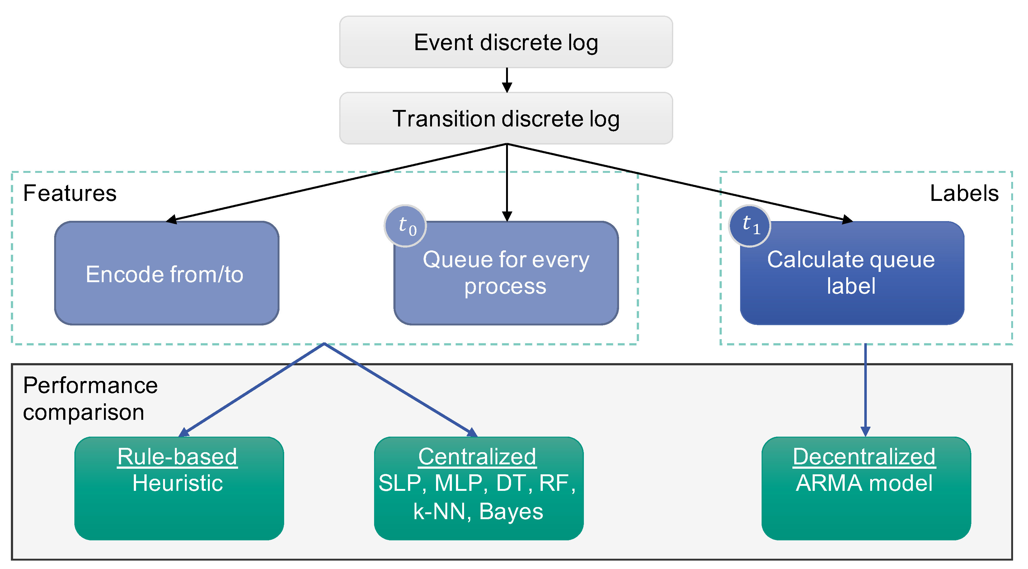
In the following section, the materials and methods are presented one by one, as these form the basis for the evaluation and the subsequent results. In Figure 1, an overview of the general approach that is followed throughout this paper is illustrated. The different models that are considered are listed in the lower part of Figure 1 and are described in detail in this section. First, in Section 2.1, the queue and its possible length are defined. Section 2.2 then describes the developed rule-based heuristic. The decentralized approach and the underlying model are presented in Section 2.3. Last but not least, different possible models for the centralized perspective are listed and discussed.
2.1. Delimitation
The aim of this paper is to predict the queue in a manufacturing system as accurately as possible using various models. Queuing theory was born in 1909 when mathematician Agner Krarup Erlang first attempted to dimension telephone exchanges [7]. In later years, more research was done in the direction of queuing theory and identified applications in many different areas. Because of the development of computer networks, the research has gained renewed importance in recent years [9]. The range of applications extends from the health care sector to transportation, shop floor design in production, to computing and beyond. Queues are also indispensable in manufacturing today [8].
In queuing theory, a node describes a place that offers a service performed by a limited number of servers to jobs. If there are more jobs at a node than there are servers, a queue of currently unserved jobs emerges. These jobs wait in the queue until it is their turn to be processed. There is a standard notation, Kendall’s notation, which has become established for queuing models [15]:
A denotes the arrival process, i.e., the distribution between two arrivals.
S denotes the service time distribution and c the corresponding number of servers.
Simple and well-known models are for example M/M/1 (single server), M/M/s (multiple servers), and M/G/1. The latter was first solved by Pollaczek in 1930. M is the abbreviation for Markov and reflects a Poisson input with exponential service times. G resembles any other possible distribution (normal distribution, equal distribution, etc.) [16].
In addition, there are different service disciplines that arrange the order in which jobs leave the queue. The most famous of these is the FIFO (First-In First-Out) principle, which is also known as the first-come-first-serve principle. If the FIFO principle is applied, the order with the longest waiting time is always served first [17].
In many manufacturing operations, products are produced using flow production or batch production, where an order passes through a predefined sequence of machines. Under these conditions, production planners can easily use the given key figures and lead times and, thus, determine buffer times and suitable queues precisely in advance. However, these conditions do not exist in complex manufacturing job shops, where identical processes can be executed by several different machines and jobs remain within the production system for a comparably long time. Due to this fact, a product can follow different routes through the factory [18]. The properties of complex manufacturing job shops are explained in more detail in Section 3.1 with reference to the case study.
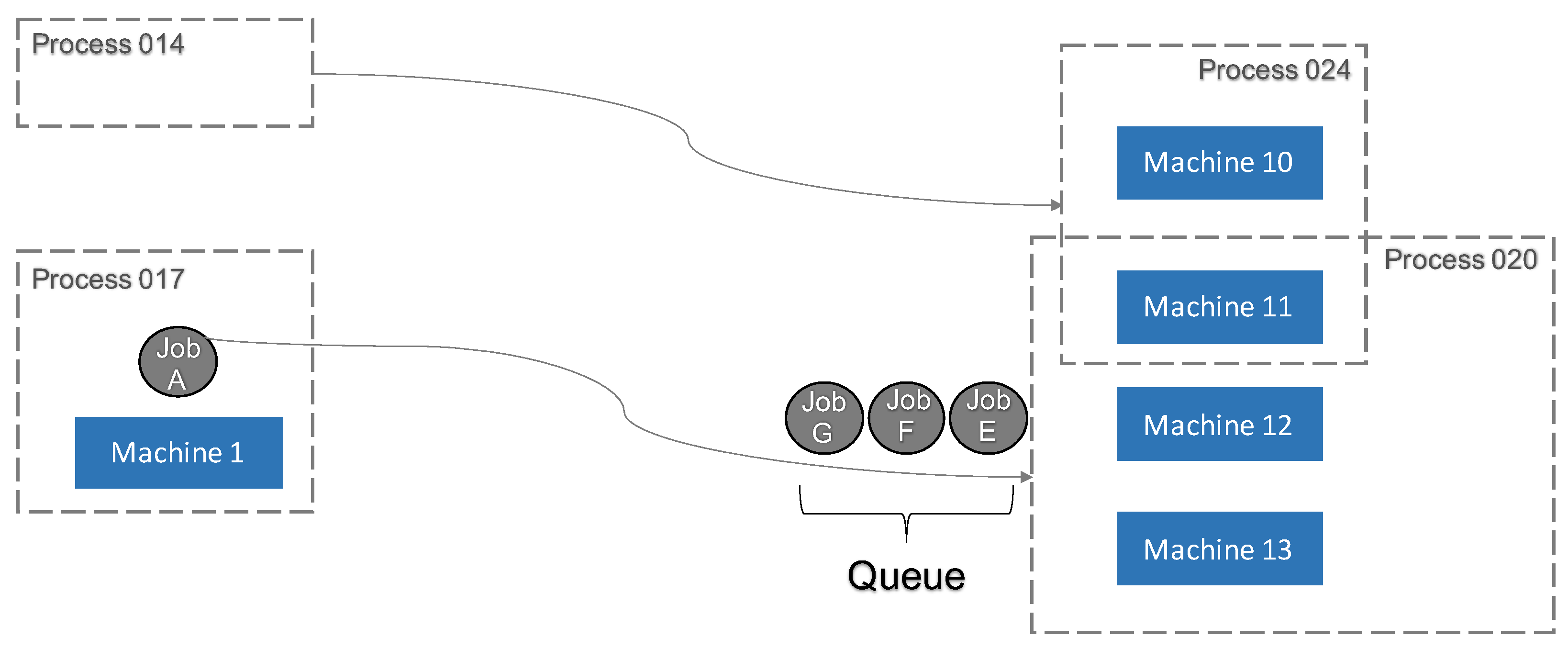
In the context of this paper, the queue definition was slightly augmented, to accommodate complex job shop manufacturing environments. Before introducing the definition, it is necessary to understand the concept of dispatching, as visualized in Figure 2: Before a job is sent to Machine 1 for processing, the length of the queue in front of the next machine (for instance, Machine 11) needs to be known. If the waiting time resulting from this queue is expected to exceed a specified time limit, it may be more favorable to skip processing those jobs and continue with jobs along a different route instead, which can thereby retain their time constraint limit. Time constraints limit the time between processing on two or more possibly consecutive machines [19]. As introduced by Little’s law, the queue length and transition time can be related, and hence, it is promising to regard queue lengths for subsequently controlling dispatching.
The main difference from other manufacturing definitions of a queue is that the newly determined queue does not map jobs in front of individual machines or connections between two specific machines. Instead, the waiting queue in front of several machines is summarized. In Figure 2, Job A is first processed by Machine 1. After finishing, depending on the specifications and properties of the product, it is mandatory to carry out the next process step within production. Since in complex manufacturing, job shops machines have the ability to run several different processes, it is not clear in advance to which machine Job A will be sent next to be processed further.
The products are therefore not distinguished or identified by a sequence of machines, but by a specific sequence of processes. If a particular process, such as Process 020 in Figure 2, has to be executed as the next step, it is very likely that more than one machine can execute this process. In the given example, these are Machines 11–13. It does not matter which of these machines processes the job; it is only important that the right process is conducted. Thus, the approach is to relate the cumulative queue to the processes rather than to machines. The characteristics of machines in complex manufacturing job shops are the ability to execute several different processes, which makes the calculation of machine-specific queues difficult. It is insufficient to consider only the jobs that are currently waiting for a given process at the next machining process. Because other machines can also execute different processes, it is possible and, therefore, very probable that there are jobs in the combined queue that have another process as the next processing step. Thus, in the example, Jobs G, F, and E are in the combined queue of Machines 11–13, which adds to the complexity of the calculation/prediction of this queue.
Regarding the problem from a different perspective, jobs that are in the combined queue of multiple processes are not processed exclusively by the same machines. For instance, consider a job waiting for Process 024 that could be performed on a machine that shares two or more processes, as is the case with Machine 11 in Figure 2. This probability, that a job waiting for a different process is not exclusively processed by the regarded machines of the initial process, can be quantitatively analyzed and was included in further analyses.
Formally, for conventional manufacturing systems, a queue at time t in front of process p can be defined as the number of all jobs j that have finished processing at a time , are currently transitioning to the next process , and will start to be processed at time in the future:
In order to calculate the newly introduced queue, we first created a mapping between machines and processes. The set of machines M for a process p is defined by all machines that can execute this process. The same is defined conversely for all processes p that can be executed by machine m:
The expanded set of subsequently relevant processes for a job j is defined as:
This finally leads to our new definition of a queue, which sums up all queue values of the expanded set of succeeding processes multiplied by their weight. This weight is defined as the percentage of machines that overlap with the machines of the initial succeeding process:
Due to the problem characteristics, there are two mutually exclusive approaches that either focus on predicting individual queue lengths based on previous information about this particular queue (decentralized) or that are based on a prediction that takes into account the entire production system state from a centralized perspective. While several machine learning models are applicable to both decentralized and centralized approaches, only the most prospective combinations are reported in the following.
2.2. Heuristic Approach
The first model for calculating the queue is the heuristic approach. To simplify its introduction, it is necessary to define the variable points of time first: is the time just before a job enters a machine. The time directly after this job has been finished in the machine is defined as . As already mentioned, the goal at is to calculate the queue at for the next process in order to be able to decide in whether the job should be dispatched or not. In the example of Figure 2, Job A will be sent to Machine 1 in . From the route description, it is known which process must be executed after Process 017. Thus, it becomes clear that the queue for Process 020 must be considered at time .
The general formula for the calculation can be stated as:
At time , all current data of the factory are assumed to be known. More precisely, it must be known where every job is located within the whole production system at that moment. With this knowledge, the queue for Process 020 can be determined easily at time . Further, Queue is simply the queue at time plus all jobs that are added to the queue from all predecessors while Job A is processed. In addition, any jobs in the queue at that finish processing and, thus, leave the queue while Job A is processed must be subtracted from the term. In the given example (Figure 2), Job E may be sent to one of Machines 11, 12, or 13 while Job A is being processed on Machine 1. Consequently, this job leaves the queue under consideration and must be deducted. At the same time, other jobs enter the queue that are finished on another machine between and and have to be processed next.
This can be used for two purposes, firstly to determine the queue lengths from a log file for all discrete time steps and, secondly, for heuristic anticipation of future queue lengths. With the assumption that a process always takes the same time to execute, this information can be used in the prediction of the process end time. We used the historical median in this case because the expected time is easily distorted by rare overlong times, which can occur in the case of problems such as machine breakdowns.
In addition to the heuristic just described and the two approaches that follow, another perspective is considered as a kind of reference method to evaluate the quality of the newly introduced approaches. This method does not try to predict the queue length for , but looks at the queue at time . The length is calculated by simply counting and adding up the waiting jobs before the next process. Thus, the approach neglects the leaving jobs and arriving jobs from Equation (7) and is hence based on the assumption that no large state changes occur between the times and . In general, this method can be declared as the current State-of-the-Art (SotA) in the determination of queue lengths.
2.3. Decentralized Approach
Besides the described heuristic in Section 2.2, two more general approaches were considered for the task of queue length forecasting. These were based on using known models and methods from statistics and machine learning. First, a decentralized approach for predicting the queue length for a single edge between two machines, or a machine and a process group, was used, and second, a centralized perspective was probed, taking all the available processes into account for the forecast.
Looking only at two consecutive processes at a time allows the usage of time series analysis for the forecasting of the queue length in front of the subsequent process [19]. For this decentralized approach, an Autoregressive Moving Average (ARMA) model was chosen to analyze and predict the sequence of queue lengths over time. Thereby, the prediction of the current value via ARMA follows Equation (8) using a sequence of predecessors and white noise [20]. The ARMA model and its prediction consist of two parts. Through a linear combination of a constant change c, a random noise , and the estimated process parameters , the Autoregressive (AR) part models the partial autocorrelation, i.e., the direct linear relationship between time steps [20]. The influence of random effects on the values over time combined with estimated process parameters is modeled by the Moving Average (MA) part [20]. Decisive for the performance of an ARMA model is the right choice of the values p and q [20]. These determine how many past time steps and noise influence the values of the time series [20]. For the task in this paper, this was determined by the selection of the past p and q queue lengths of the chosen edge. These can be deduced by looking at autocorrelation and partial autocorrelation plots.
The second model applied in the decentralized approach uses weighted averages. Exponential smoothing is used for this purpose, which was introduced by Holt and Winter in the late 1960s [21,22]. Many other successful forecasting methods have been derived from this initial research. The Simple Exponential Smoothing (SES) model is one of the easiest ways to forecast a time series [23]. Its forecasts are weighted averages of past observations, which are increasingly discounted the older the observed values are [24]. Accordingly, more recent observations have a greater influence on the prediction than older ones. A disadvantage of the simple exponential smoothing model in its standard model is that it cannot deal with trends or seasonality [24]. The forecast of value ŷ can be any given data, for example the future demand that is an estimation of the actually observed demand y. We initialized the very first forecast as zero and the second forecast as the value of the first observation. When the time t is greater than 1, the formula of the simple exponential smoothing model is:
can be set arbitrarily and has a great influence on the prediction performance. When approaches 1, the first part of the formula becomes larger, and the focus is on the most recent observations. On the opposite side, if is lower, there is more weight on the last forecast . Setting creates a tradeoff between a forecast that can quickly adjust to short-term changes and a forecast that is not too sensitive to noise and outliers [24].
2.4. Centralized Approach
For the centralized approach, different supervised machine learning models are applied for the forecasting task. Thereby, the centralized perspective takes all possible edges between the different manufacturing processes at a given time into account. Here, the most commonly used algorithms discussed in the literature for predicting numerical values were chosen and studied in detail.
Generally, in supervised machine learning, a model tries to predict a specific target value of a given data set [25]. This set usually contains selected relevant information on which the model is trained [25], so that labeled input-output pairs can be used. Through a model-specific learning process, the target value is predicted and compared with the label included in the data set [25]. If the true value and prediction deviate, the model adapts automatically to achieve a better result in the next run [25], based on a predetermined loss function, which relates to this deviation. The selection and generation of relevant input features for the training are some of the first and also most important steps for machine learning [25]. As mentioned in the previous subsections, the overall goal of this paper was to determine methods to forecast the queue length for forward from the point . Therefore, an important input for the training of the different algorithms is the exact knowledge about the current state of the processes. In other words, the queue length at in front of the next process step need to be provided as an input. The values can be generated as described in Section 2.1. Following the calculation of these values, they are adjusted by multiplication with the fraction of relevant machines. This adjustment is necessary to get more accurate results since the queue length was previously calculated for a wider range of machines (see Section 2.1). The current state is also described through another second input feature by counting the queue length in front of every possible process step. To facilitate quick learning, these values require normalization. By applying one-hot-encoding, the starting and target process are fixed. The three given features together with a previously determined queue length as the label represent the data set for training the models. Finally, testing on previously unseen data and a comparison of the results with the true values of the queue lengths allows the evaluation of the performance of the considered models.
2.4.1. Decision Tree
A Decision Tree (DT) is the recursive partitioning of a data space to determine a discrete or continuous value for a given instance [26]. In so-called internal nodes, different logical rules are applied to split the given data into groups [27]. At the lowest level of the tree, the leaf nodes, the target value for the instance is assigned [27]. If the target value like for the task of this paper is continuous, so-called regression trees are used for the prediction [26]. For the decision on which of the given features the split is based, the most informative one has to be determined [27]. Regression trees usually use the feature with the greatest reduction in the sum of squared differences for the split (entropy) [28]. Normally, the application of decision trees on regression tasks relies on the assumption of a linear relationship in the data [28]. Such a relationship for queue length forecasting is quite possible, which motivates the use of this model.
The limitation to model only linear relationships and the tendency to overfit quite fast [27], despite reducing the DT size through so-called pruning, could also be significant disadvantages in the use of decision trees for the task. For this reason, among others, further models must be considered and are discussed in the following.
2.4.2. Random Forest
A Random Forest (RF) relies on the idea of ensemble learning [29]. The algorithm combines different decision trees for classification or regression tasks, using two kinds of randomization methods to generate and train these trees [29]. First, a technique called “bootstrap aggregating (bagging)” is applied [29]. Through this technique, training samples are generated by drawing with replacement from the original dataset [30]. The second randomization relies on training the decision trees only on a random subset of the available features [29]. The application of these two methods of randomization yields different results for the target value [29]. The ultimate prediction of a random forest is then achieved by the aggregation of the different results from the trees to one final value [31]. In the end, the forecast of the queue lengths by using the random forest algorithm is given by the arithmetic mean of the different generated results from the decision trees.
2.4.3. Bayesian Regression
In contrast to a classical point estimation of the unknown weights of a regression model, the Bayesian approach relies on the usage of probability distributions to characterize the uncertainty of weights [32]. In other words, the aim of Bayesian regression is not to find a single “best” value for the model parameters, but a posterior distribution. This posterior distribution is conditional and calculated by multiplying the likelihood of the data with the prior probability of the parameters and divided by a normalization constant [33]. The concept behind this is the Bayesian inference, using the Bayesian theorem [32]. As mentioned previously, this approach allows including the uncertainty of the desired prediction, which is also the main advantage of the model [32].
2.4.4. Single-Layer Perceptron
A single-layer perceptron (SLP) constitutes the simplest neural network and the key element of other more complex networks [34]. The basic concept of a neural network is that input values are multiplied by learned weights, then combined within nodes and layers and aggregated to an output via an activation function [34]. In these models, the learning process is typically based on the idea of the backpropagation algorithm [35]. Thereby, the input weights are updated regularly based on a potential deviation between the predicted value and the label [35]. To find the optimal weights with the least deviation within the solution space, a variety of optimization algorithms exist currently. One of the most popular and promising is adaptive moment estimation [36], which is applied here. Another important factor for the successful application of neural networks is the right choice of the previously mentioned activation function [37]. These define the output of a node for a given input [37]. In recent years, many different functions have become increasingly popular, in contrast to the original sigmoid function, such as the rectified linear activation function (ReLU) [37]. The biggest advantage of ReLU is that it solves the vanishing gradient problem [38]. Like in some of the previously described models, the typical SLP is a linear model, but through the application of ReLU as the activation function in the output, the model is able to map non-linear behavior [37]. Therefore, an SLP model was also considered and evaluated for the task of queue length forecasting.
2.4.5. Multi-Layer Perceptron
Adding one or more additional layers with an arbitrary number of neurons between the input and output of an SLP leads to more general non-linear models, the Multi-layer Perceptrons (MLPs) [34]. The structure and interconnection of MLPs are usually organized in a feedforward way [34]. These feedforward networks are neural networks in which the so-called nodes are fully connected and the information flows only in one direction [39]. The additional layers are also known as hidden layers and are the key aspect for deep learning neural networks [40]. Due to the danger of overfitting and the desire to keep the models as basic as possible (Occam’s razor), only simple neural networks with a single hidden layer were tested in the scope of this paper. Thus, deep learning was not considered further for the task of queue length forecasting. For the MLP model in this paper, the activation function and optimization algorithm remained similar to the SLP model.
2.4.6. k-Nearest Neighbor
Contrary to the other previously described machine learning models, the technique of k-Nearest Neighbor (k-NN) is a nonparametric, instance-based approach [41]. The prediction of the value of a new instance is performed by looking at the k-nearest neighbors with the smallest distance to the currently considered data point(s) [41]. The most commonly used norm for calculating this distance is the Euclidean distance, which was also the chosen approach in this paper. Numeric values can be predicted by calculating the arithmetic mean of the k-nearest neighbors and assign the result to the instance under investigation [42]. Therefore, for the task of forecasting the queue length in front of a process for a future point in time, this can be achieved by taking the average over the values of the k-nearest neighbors of the process.
3. Results
This section presents the results of the individual approaches and methods. Real data from a semiconductor manufacturer were used to obtain conclusions that were relevant to practical applications. In addition, the results were compared by calculating statistical key figures for all used models.
3.1. Case Study Introduction
The models and approaches discussed in Section 2 were tested in a case study. The data with which the analyses were carried out and that were used as the input for the models came from a large semiconductor manufacturer and spanned several weeks. The semiconductor industry is very well suited for the analyses of complex manufacturing job shops because this fulfills all the characteristics of complex manufacturing job shops due to the highly complex production with several hundred sequential processes per job and many machines. The production of a microchip includes four basic steps: wafer fabrication, probing, packaging, and final tests [43]. The focus of the case study was on the most time-consuming part, wafer fabrication, where many chemical processes are performed. The machines for carrying out the various processes are highly sophisticated and typically extremely expensive [43]. In addition, semiconductor manufacturing is a perfect example and also a role model for Industry 4.0 [18], leading to the availability of such data.
First, essential terms used to understand the data were introduced, as these were used in the following to present the results. A lot is an order that passes through production and is processed on machines. For simplification, it was assumed that only one lot can be processed on a machine at a time. To show the order of magnitude in the data considered from one month, a few million lots were processed on approximately 1000 machines. Another important element is the operations, which are numbered and, thus, traceable. An operation number signifies a special work step, e.g., cleaning. What is special about semiconductor manufacturing is that the machines can usually run several different operations, which makes scheduling very difficult [18]. The last term is the route. A route is a sequence of many operation numbers that must be performed to produce a microprocessor. It is important to note that the route is related to operations (processes) and not to machines. Because an operation can be processed by several machines, it is possible that two identical products are processed by completely different machines during their route through production [18].
In addition to the features already mentioned, there are a few more that make producing semiconductor chips more difficult. The flow through the factory is in no way similar to a line production as it is applied in many industries. It is even possible for lots to return to machines on which they were processed earlier in the production process. This phenomenon is also called re-entrant flow in technical jargon [18]. The process that a machine executes may differ within a short time. Depending on the operation, a setup time must be planned. These setup times can vary strongly from operation to operation [43]. The next problem is frequent machine breakdowns, which are unpredictable, occur spontaneously, and are thus hard to manage. Besides, the machines have an influence on several queues or are networked to different extents. A failure or breakdown of a highly networked machine can therefore cause great damage. Additionally, there are time constraints between certain operations during production [19]. Time constraints are upper time limits to the time that a lot may stay between two machines without being processed. Because complicated chemical reactions and processes are run during wafer fabrication and because the wafers are unimaginably thin, natural phenomena can cause the surface of the wafers to change as they lie around without being processed [44].
To avoid these physical changes, time constraints are set between key operations. Therefore, like the routes, the time constraints also refer to the processes and not to the machines. If time constraints are broken, the affected lots must either be reprocessed or even disposed, resulting in high costs for the manufacturer [44]. A cleanroom must be present most of the time during wafer fabrication so that the surface quality of the sensitive wafers is maintained and automated material flow impeded. This means that a certain temperature and humidity must prevail, and the air has to be dust-free. To meet the time constraints, it is eminently important to predict the queue as accurately as possible. If during dispatching at time it becomes clear that the next time constraint cannot be met anyway because of an overlong queue, the lot can be thrown away directly or still protected to save high costs. This prediction of the queue was tested and evaluated in the next section on the existing data using the models presented in Section 2.
3.2. Metrics
We evaluated our models against the SotA described in Section 2.2 using four metrics that are commonly used for measuring the performance of regression models. The Mean Absolute Error (MAE), Mean Squared Error (MSE), and Root Mean Squared Error (RMSE) (Equations (10)–(12)) measure the absolute and squared deviation of the model’s n predictions to the actual values . While the MAE describes the average error alone, the MSE and RMSE are additionally influenced by the variability of the underlying data [45]. Finally, the R-squared metric (Equation (13)) is calculated to relate the mean squared error to the variance of the data set. For linear models, this value lies between zero and one and specifies the percentage of variability in data that is explained by the model. For non-linear regressions, however, the metric can be negative and does not have an explanatory value [46].
3.3. Training
We applied our decentralized approach to two different transitions, consisting of several thousand transitioning lots over the period of one month. Our data set for the centralized approach consisted of about a hundred thousand transitions, of which 80% were used for training and 20% for validation. Due to the large number of processes and since we applied a one-hot encoding for both the start and destination process, our feature count was in the thousands.
The neural network models were trained for 10 epochs respectively using the Adam optimizer with a learning rate of 0.001 and a batch size of 256, in order to obtain good values and avoid overfitting. The MLP models consisted of one hidden layer with between 10 and 100 neurons. For the loss function, we used the mean absolute error. We varied the maximum depth of our tree-based models among five, ten, and no limit and trained the random forest regressor using 50, 100, and 200 estimators. Finally, we varied the number of neighbors of the k-NN regressor between five and one hundred.
3.4. Comparison
3.4.1. Heuristic
The heuristic approach performed quite badly, which clearly showed the inferiority of rule-based decision systems for the regarded use case. As can be seen by the value in Table 1, the variance of the predicted values was more than thrice as much as the variance of the actual values, which means that just using the mean as the prediction would lead to a better result.
A clear connection can be seen between the prediction time horizon and the quality of the predictions. For example, limiting the maximum allowed process time, i.e., , to three hours resulted in an MAE of , which was half of the original value. In general, the rule-based model overpredicted the actual value when the processing time was too long or the actual queue value was higher than approximately 50.
3.4.2. Decentralized Models
For both transition types, the decentralized approach yielded decent predictions, as can be seen in Table 2. The ARMA model produced slightly better results than the SES model. However, the models performed worse than the state-of-the-art in every metric. This can be explained by the fact that the SotA result used the production system state at , while the decentralized approaches were only given the state of the last job that had been sent along the transition. The resulting queue values from both production states were only identical if both the preceding and current job were processed subsequently on the same equipment, as in this case was equal to , i.e., the time the last job left the equipment. In any other case, lied further in the past and thus increased the time horizon of the prediction.
3.4.3. Centralized Models
The results of centralized models are summarized in Table 3, where five out of six models performed better than the state-of-the-art. All tested model variations can be found in the Appendix in Table A1, Table A2, Table A3 and Table A4.
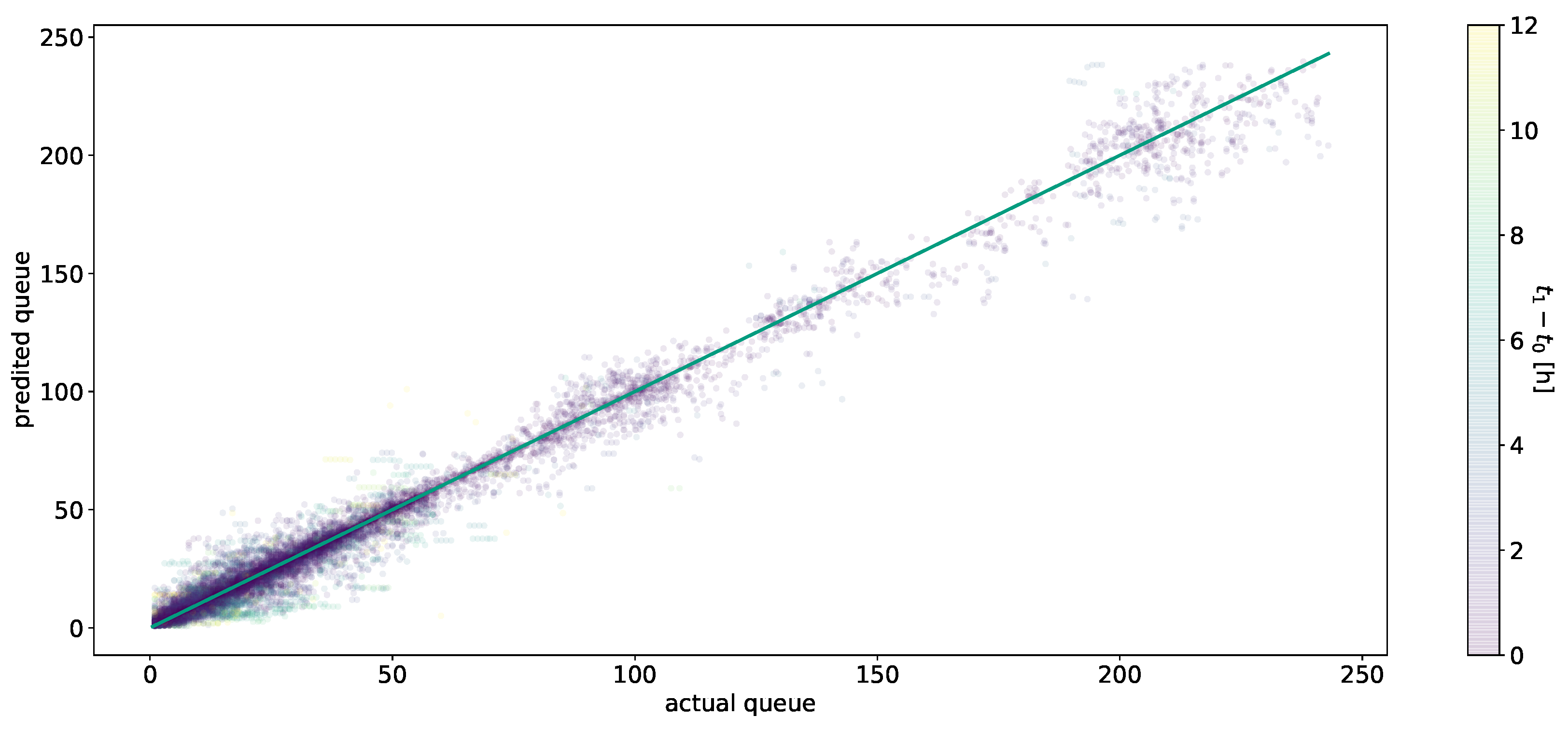
The neural network-based approaches performed overall the best out of all tested approaches. The SLP model without any hidden layers surprisingly beat all MLP models (see Table A1), which tended to overfit during training. Figure 3 shows the predicted values versus the actual values, with values on the green line being optimal. The residuals can be obtained by looking at the distance between the data points and the diagonal. For queue lengths smaller than 60, most of the predictions were very close to the diagonal, meaning a very low prediction error. Higher queue values occurred far less frequently, and we saw for these values an increased prediction error on average. Regarding the heuristic model, predictions with a greater time horizon, which are colored in green or yellow, tended to yield worse results. In general, we did not see any systematic errors in the predictions, which indicated together with the MAE of a small amount of uncertainty for the SLP model.
Regarding our use case, it has to be noted that underpredicting the queue value was more costly than an overprediction. This was the case because a dispatching decision based on a too low queue count could lead to a violation of the time constraints and as a consequence higher reprocessing costs, as explained in Section 3.1. However, all our models do not distinguish between both cases at the moment.
Interestingly, using the neural models to calculate even just the queue value at from the given data turned out to be a more challenging task than expected. Training led to similar error values as the prediction of the queue at , even though the former was strongly related to the input features. This could indicate that the simple machine learning approaches that were exploited in this use case were not sophisticated enough to handle the high dimensionality of our data set in conjunction with the complex relationships between different machines and processes.
All tree-based approaches were challenged regarding their prediction ability of our queue feature. The strength of the decision trees and random forest regressors in finding the most relevant and important features could not be used to their advantage as both the one-hot encodings, as well as the given queue counts of every process were highly relevant for predicting the label. This either resulted in very large and complex trees, which led to overfitting or led to the omission of important features, which in both cases meant an overall worse performance. Limiting the maximum depth of the decision tree regressor to ten, whose results are presented in Table A2, actually yielded better results than not limiting the depth at all, which clearly showed the compromise between overfitting and feature omission. Additionally, pruning can be adjusted.
The random forest models performed overall better than equally deep decision trees, which was expected given that a random forest uses the result of multiple estimators and, thus, overcomes the linearity restriction. The best random forest model slightly beat the SotA regarding the MAE, but overall, the models reached their limits, as can be seen in Table A3. We also varied the number of estimators from 100 to 50 and 200, which is shown in Table 3, but did not see an improvement in performance.
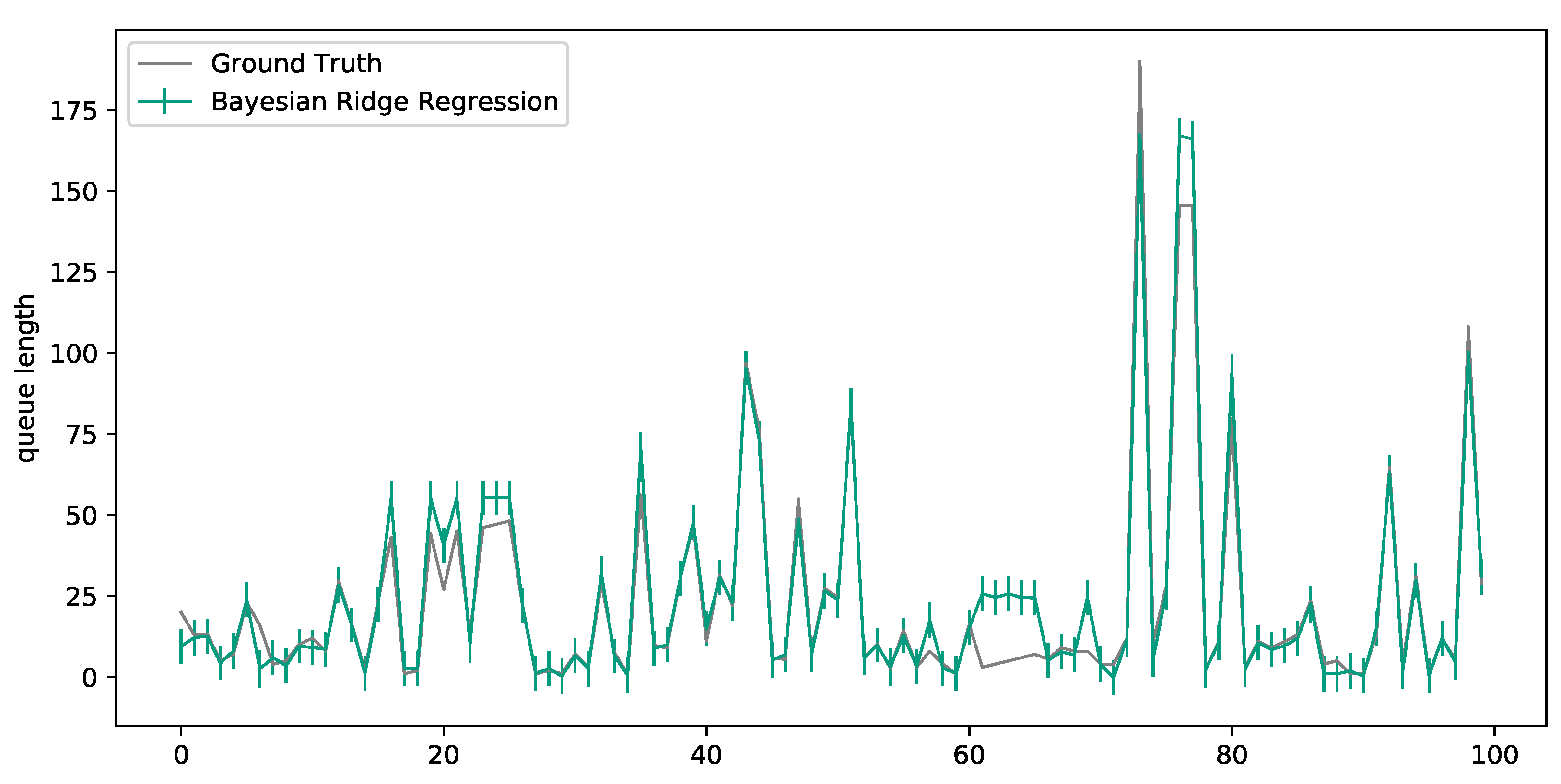
Out of the non-neural machine learning models, only the Bayesian ridge regression performed better than the state-of-the-art and even achieved an identical R-squared value as both the SLP and MLP. Being a linear regression model and thus very similar to the SLP model, this may not be that surprising; however, with the large number of features, the model was not expected to perform well. Furthermore, Figure 4 shows that the prediction uncertainty was relatively low where, on average, the standard deviation of the probabilistic model was 5.38.
The best k-nearest neighbor regressor performed slightly worse than the neural approaches, but beat all tree-based models, as well as the Bayesian ridge regression. Table A4 shows that increasing the number of neighbors yielded a better performance, but only to a certain degree. One explanation could be that there were too few training samples for the instance-based approach to correctly infer a correct result for every possible combination of a transition and production state. For example, there could likely have been none or only very few instances for a given transition in our training data, which would mean that the nearest found neighbor was completely irrelevant for the given production state. The model would thus require a far greater number of training entries, which however in turn would greatly compromise its runtime performance and make its employment impractical.
4. Discussion
All in all, the proposed machine learning-based queue length prediction for complex manufacturing job shops outperformed the SotA approaches. Nevertheless, several of the analyzed models performed significantly worse, albeit the SLP and Bayes approach showing strong results, a comprehensive comparison across different use cases has not yet been shown. Additionally, the area of machine learning provides a plethora of interesting approaches that in some cases have the potential to provide good results as well, but have so far not been included. Many of the regarded approaches also feature a variety of optimization, modeling, and hyper-parameter tuning approaches, such as neural networks, that cannot efficiently be regarded all at once. Thus, it is promising to include successors of the currently best performing models, such as convolutional neural networks or graph neural networks. In particular, approaches that have been applied in different domains, such as traffic prediction [47], should be regarded.
However, this paper is among the first to approach the forecasting of queue lengths by machine learning means in the area of semiconductor manufacturing and beyond. Thus, the improvements can yield further studies to relate queue length information to key performance indicators and thereby help to alleviate the complexities of complex job shops. In particular, currently, manually performed jobs can be automated. Likewise, more computing power and the inclusion of probabilistic information about future queue behavior have the potential to improve the results in follow-up studies. Hence, the main contribution of this paper lies in the application of forecasting, as well as further machine learning models and the modeling of real-world complex manufacturing systems.
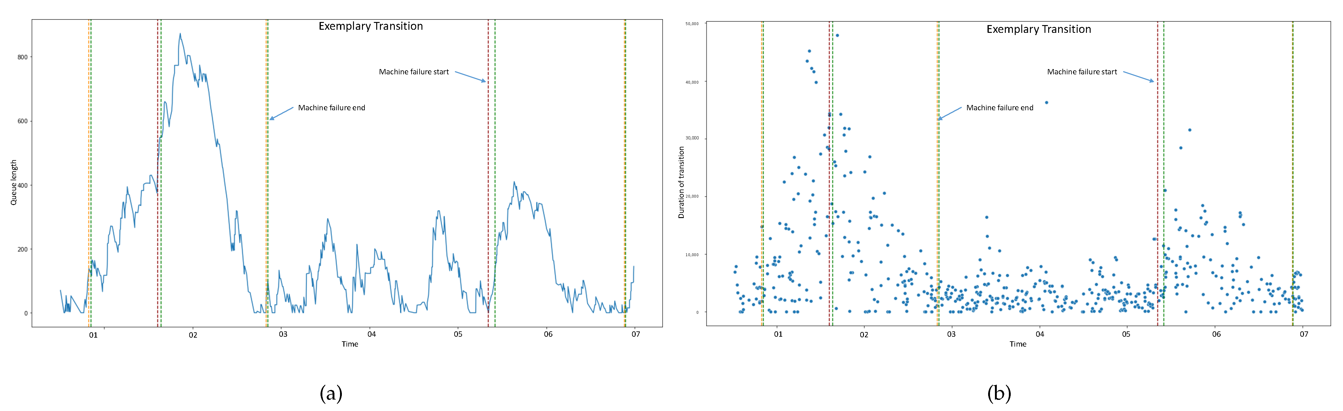
One of the most promising problems to be tackled with the presented methods is the improvement of time constraint adherence in semiconductor manufacturing. Moreover, the general queue length reduction can be facilitated by better predictions. One way to do so could be the inclusion of information about nodal events, such as machine breakdowns. As shown in Figure 5, failure events and queue length by visual comparison can have a strong influence on transition times and the length of queues themselves.
5. Conclusions
In a nutshell, predicting queue lengths in manufacturing systems can, by feasible forecasting and machine learning techniques, significantly be improved over the state-of-the-art. Owing to the long known relation of queue lengths to various manufacturing-specific key performance indicators, this information in turn can be used to optimize production. Within this study, several easy-to-implement forecasting methods for this queue length prediction were presented within a framework that showed how to approach this and similar problems. The methods were then validated in a real-world case study showing an edge over the state-of-the-art for several of the presented models. As a result of the analyses and comparisons of the different models, it can be stated that the single-layer perceptron performed best in our case study. Therefore, we recommend this model, but it is not a guarantee that it has the best performance in every use case. In general, predictive models as elaborated in the paper can be applied to inventory level-based production systems. For example, they can help human workers to make important allocation decisions in order to produce as efficiently as possible. In future studies, it seems worthwhile to analyze further approaches, such as convolutional neural networks or long short-term memory networks, as well as to use accurate queue length information for improvements in the control and design of the corresponding manufacturing system.
Author Contributions
Conceptualization, M.C.M., L.S. and G.L.; methodology, M.C.M., A.A., M.D.F. and F.M.; software, A.A., M.D.F. and F.M.; validation, M.C.M., A.A., M.D.F. and F.M.; formal analysis, M.C.M.; investigation, M.C.M., A.A., M.D.F. and F.M.; resources, M.C.M.; data curation, A.A., M.D.F. and F.M.; writing—original draft preparation, M.C.M., A.A., M.D.F. and F.M.; writing—review and editing, M.C.M., L.S. and G.L.; visualization, A.A., M.D.F. and F.M.; supervision, G.L. All authors read and agreed to the published version of the manuscript.
Funding
This research work was undertaken in the context of DIGIMAN4.0 project (“DIGItal MANufacturing Technologies for Zero-defect Industry 4.0 Production”, http://www.digiman4-0.mek.dtu.dk/, accessed on 31 March 2021). DIGIMAN4.0 is a European Training Network supported by Horizon 2020, the EU Framework Programme for Research and Innovation (Project ID: 814225).
Institutional Review Board Statement
Not applicable.
Informed Consent Statement
Not applicable.
Data Availability Statement
Not applicable.
Conflicts of Interest
The authors declare no conflict of interest.
Abbreviations
The following abbreviations are used in this manuscript:
| ARMA | Autoregressive Moving Average |
| DT | Decision Tree |
| FIFO | First-In First-Out |
| k-NN | k-Nearest Neighbor |
| MAE | Mean Absolute Error |
| MLP | Multi-layer Perceptron |
| MSE | Mean Squared Error |
| ReLU | Rectified Linear Unit |
| RF | Random Forest |
| RMSE | Root Mean Squared Error |
| SES | Simple Exponential Smoothing |
| SotA | State-of-the-Art |
| SLP | Single-Layer Perceptron |
Appendix A. Queue Distribution
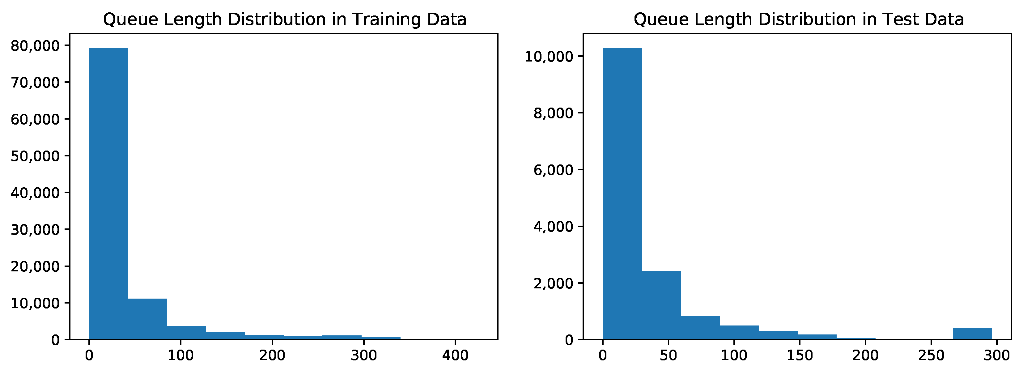
The following Figure A1 shows the distribution of queue lengths in the training and test data used in the presented case study to verify no structural biases.
Figure A1.
Queue length distribution in training and test data.

Appendix B. Results
The following tables show different parameter variations for our presented models.

Table A1.
Results for a single-layer perceptron and several multi-layer perceptrons with different numbers n of nodes and one hidden layer. The bold is the best result.
Table A1.
Results for a single-layer perceptron and several multi-layer perceptrons with different numbers n of nodes and one hidden layer. The bold is the best result.
| Metric | SotA | SLP | MLP (n = 10) | MLP (n = 25) | MLP (n = 50) | MLP (n = 100) |
|---|---|---|---|---|---|---|
| MAE | 3.201 | 2.773 | 2.774 | 2.801 | 2.801 | 2.804 |
| MSE | 31.328 | 28.825 | 28.852 | 29.254 | 29.057 | 29.012 |
| RMSE | 5.597 | 5.369 | 5.371 | 5.409 | 5.390 | 5.386 |
| R2 | 0.980 | 0.982 | 0.982 | 0.981 | 0.982 | 0.982 |
Table A2.
Results for the decision tree regressors, varying the maximum depth d. The bold is the best result.
Table A2.
Results for the decision tree regressors, varying the maximum depth d. The bold is the best result.
| Metric | SotA | DT (d = 5) | DT (d = 10) | DT (d = 20) | DT (d = ∞) |
|---|---|---|---|---|---|
| MAE | 3.201 | 3.472 | 3.385 | 3.620 | 4.934 |
| MSE | 31.328 | 40.272 | 45.495 | 55.495 | 72.890 |
| RMSE | 5.597 | 6.346 | 6.745 | 7.450 | 8.538 |
| R2 | 0.980 | 0.975 | 0.971 | 0.965 | 0.954 |
Table A3.
Results for the random forest models, varying the maximum depth d (keeping the number of estimators at 100) or number n of estimators (keeping the maximum tree depth at ∞). The bold is the best result.
Table A3.
Results for the random forest models, varying the maximum depth d (keeping the number of estimators at 100) or number n of estimators (keeping the maximum tree depth at ∞). The bold is the best result.
| Metric | SotA | RF (d = 5) | RF (d = 10) | RF (d = ∞) | RF (n = 50) | RF (n = 200) |
|---|---|---|---|---|---|---|
| MAE | 3.201 | 3.174 | 3.105 | 3.211 | 3.306 | 3.244 |
| MSE | 31.328 | 32.938 | 34.597 | 32.449 | 35.869 | 34.539 |
| RMSE | 5.597 | 5.739 | 5.882 | 5.696 | 5.989 | 5.877 |
| R2 | 0.980 | 0.979 | 0.978 | 0.980 | 0.977 | 0.978 |
Table A4.
Results for the k-NN models, varying the number of nearest neighbors k. The bold is the best result.
Table A4.
Results for the k-NN models, varying the number of nearest neighbors k. The bold is the best result.
| Metric | SotA | 5-NN | 10-NN | 20-NN | 50-NN | 100-NN |
|---|---|---|---|---|---|---|
| MAE | 3.201 | 3.249 | 3.097 | 3.007 | 2.938 | 2.936 |
| MSE | 31.328 | 35.397 | 32.357 | 30.826 | 29.656 | 29.670 |
| RMSE | 5.597 | 5.950 | 5.688 | 5.552 | 5.446 | 5.447 |
| R2 | 0.980 | 0.978 | 0.980 | 0.981 | 0.981 | 0.981 |
References
- Sinha, A.; Bernardes, E.; Calderon, R.; Wuest, T. Digital Supply Networks: Transform Your Supply Chain and Gain Competitive Advantage with Disruptive Technology and Reimagined Processes; McGraw Hill Professional: New York, NY, USA, 2020. [Google Scholar]
- Kapp, V.; May, M.C.; Lanza, G.; Wuest, T. Pattern Recognition in Multivariate Time Series: Towards an Automated Event Detection Method for Smart Manufacturing Systems. J. Manuf. Mater. Process. 2020, 4, 88. [Google Scholar] [CrossRef]
- May, M.C.; Overbeck, L.; Wurster, M.; Kuhnle, A.; Lanza, G. Foresighted digital twin for situational agent selection in production control. Procedia CIRP 2021, 99, 27–32. [Google Scholar] [CrossRef]
- Greschke, P.; Schönemann, M.; Thiede, S.; Herrmann, C. Matrix structures for high volumes and flexibility in production systems. Procedia CIRP 2014, 17, 160–165. [Google Scholar] [CrossRef] [Green Version]
- May, M.C.; Kiefer, L.; Kuhnle, A.; Stricker, N.; Lanza, G. Decentralized Multi-Agent Production Control through Economic Model Bidding for Matrix Production Systems. Procedia CIRP 2021, 96, 3–8. [Google Scholar] [CrossRef]
- Wu, K.; McGinnis, L. Performance evaluation for general queueing networks in manufacturing systems: Characterizing the trade-off between queue time and utilization. Eur. J. Oper. Res. 2012, 221, 328–339. [Google Scholar] [CrossRef]
- Erlang, A.K. The theory of probabilities and telephone conversations. Nyt. Tidsskr. Mat. Ser. B 1909, 20, 33–39. [Google Scholar]
- Roy, D. Semi-open queuing networks: A review of stochastic models, solution methods and new research areas. Int. J. Prod. Res. 2016, 54, 1735–1752. [Google Scholar] [CrossRef]
- Little, J.D. OR FORUM—Little’s Law as viewed on its 50th anniversary. Oper. Res. 2011, 59, 536–549. [Google Scholar] [CrossRef] [Green Version]
- Chang, P.C.; Hieh, J.C.; Liao, T.W. Evolving fuzzy rules for due-date assignment problem in semiconductor manufacturing factory. J. Intell. Manuf. 2005, 16, 549–557. [Google Scholar] [CrossRef]
- Kraus, M.; Feuerriegel, S. Forecasting remaining useful life: Interpretable deep learning approach via variational Bayesian inferences. Decis. Support Syst. 2019, 125, 113100. [Google Scholar] [CrossRef]
- Mawson, V.J.; Hughes, B.R. Deep learning techniques for energy forecasting and condition monitoring in the manufacturing sector. Energy Build. 2020, 217, 109966. [Google Scholar] [CrossRef]
- Wang, J.; Zhang, J. Big data analytics for forecasting cycle time in semiconductor wafer fabrication system. Int. J. Prod. Res. 2016, 54, 7231–7244. [Google Scholar] [CrossRef]
- Wang, J.; Zhang, J.; Wang, X. Bilateral LSTM: A two-dimensional long short-term memory model with multiply memory units for short-term cycle time forecasting in re-entrant manufacturing systems. IEEE Trans. Ind. Inform. 2017, 14, 748–758. [Google Scholar] [CrossRef]
- Kendall, D.G. Stochastic processes occurring in the theory of queues and their analysis by the method of the imbedded Markov chain. Ann. Math. Stat. 1953, 24, 338–354. [Google Scholar] [CrossRef]
- Cooper, R.B. Queueing theory. In Proceedings of the ACM’81 Conference; Association for Computing Machinery: New York, NY, USA, 1981; pp. 119–122. [Google Scholar]
- Zhang, H. Service disciplines for guaranteed performance service in packet-switching networks. Proc. IEEE 1995, 83, 1374–1396. [Google Scholar] [CrossRef] [Green Version]
- Waschneck, B.; Altenmüller, T.; Bauernhansl, T.; Kyek, A. Production Scheduling in Complex Job Shops from an Industry 4.0 Perspective: A Review and Challenges in the Semiconductor Industry. In Proceedings of the SAMI40 Workshop at i-KNOW ’16, Graz, Austria, 18–19 October 2016; pp. 1–12. [Google Scholar]
- May, M.C.; Maucher, S.; Holzer, A.; Kuhnle, A.; Lanza, G. Data Analytics for Time Constraint Adherence Prediction in a Semiconductor Manufacturing Use-Case. Procedia CIRP 2021, in press. [Google Scholar]
- Chatfield, C. Time-Series Forecasting; CRC Press: Boca Raton, FL, USA, 2000. [Google Scholar]
- Holt, C.C. Forecasting seasonals and trends by exponentially weighted moving averages. Int. J. Forecast. 2004, 20, 5–10. [Google Scholar] [CrossRef]
- Winters, P.R. Forecasting sales by exponentially weighted moving averages. Manag. Sci. 1960, 6, 324–342. [Google Scholar] [CrossRef]
- Ostertagova, E.; Ostertag, O. Forecasting using simple exponential smoothing method. Acta Electrotech. Inform. 2012, 12, 62. [Google Scholar] [CrossRef]
- Hyndman, R.J.; Athanasopoulos, G. Forecasting: Principles and Practice; OTexts: Melbourne, Australia, 2018. [Google Scholar]
- Alpaydin, E. Introduction to Machine Learning; MIT Press: Cambridge, MA, USA, 2020. [Google Scholar]
- Loh, W.Y. Classification and regression trees. Wiley Interdiscip. Rev. Data Min. Knowl. Discov. 2011, 1, 14–23. [Google Scholar] [CrossRef]
- Kotsiantis, S.B. Decision trees: A recent overview. Artif. Intell. Rev. 2013, 39, 261–283. [Google Scholar] [CrossRef]
- Sutton, C.D. Classification and regression trees, bagging, and boosting. Handb. Stat. 2005, 24, 303–329. [Google Scholar]
- Breiman, L. Random forests. Mach. Learn. 2001, 45, 5–32. [Google Scholar] [CrossRef] [Green Version]
- Breiman, L. Bagging predictors. Mach. Learn. 1996, 24, 123–140. [Google Scholar] [CrossRef] [Green Version]
- Liaw, A.; Wiener, M. Classification and regression by randomForest. R News 2002, 2, 18–22. [Google Scholar]
- Bishop, C.M.; Tipping, M.E. Bayesian regression and classification. Nato Sci. Ser. Sub Ser. III Comput. Syst. Sci. 2003, 190, 267–288. [Google Scholar]
- Tipping, M.E. Bayesian inference: An introduction to principles and practice in machine learning. In Summer School on Machine Learning; Springer: Berlin/Heidelberg, Germany, 2003; pp. 41–62. [Google Scholar]
- Bishop, C.M. Neural Networks for Pattern Recognition; Oxford University Press: Oxford, UK, 1995. [Google Scholar]
- Svozil, D.; Kvasnicka, V.; Pospichal, J. Introduction to multi-layer feed-forward neural networks. Chemom. Intell. Lab. Syst. 1997, 39, 43–62. [Google Scholar] [CrossRef]
- Kingma, D.P.; Ba, J. Adam: A Method for Stochastic Optimization. arXiv 2017, arXiv:cs.LG/1412.6980. [Google Scholar]
- Sharma, S. Activation functions in neural networks. Towards Data Sci. 2017, 6, 310–316. [Google Scholar]
- Ide, H.; Kurita, T. Improvement of learning for CNN with ReLU activation by sparse regularization. In Proceedings of the 2017 International Joint Conference on Neural Networks (IJCNN), Anchorage, AK, USA, 14–19 May 2017; pp. 2684–2691. [Google Scholar]
- Cheng, B.; Titterington, D.M. Neural networks: A review from a statistical perspective. Stat. Sci. 1994, 9, 2–30. [Google Scholar]
- Schmidhuber, J. Deep learning in neural networks: An overview. Neural Netw. 2015, 61, 85–117. [Google Scholar] [CrossRef] [Green Version]
- Keller, J.M.; Gray, M.R.; Givens, J.A. A fuzzy k-nearest neighbor algorithm. IEEE Trans. Syst. Man Cybern. 1985, 4, 580–585. [Google Scholar] [CrossRef]
- Cover, T. Estimation by the nearest neighbor rule. IEEE Trans. Inf. Theory 1968, 14, 50–55. [Google Scholar] [CrossRef] [Green Version]
- Johri, P.K. Practical issues in scheduling and dispatching in semiconductor wafer fabrication. J. Manuf. Syst. 1993, 12, 474–485. [Google Scholar] [CrossRef]
- Lima, A.; Borodin, V.; Dauzère-Pérès, S.; Vialletelle, P. A sampling-based approach for managing lot release in time constraint tunnels in semiconductor manufacturing. Int. J. Prod. Res. 2020, 56, 860–884. [Google Scholar] [CrossRef]
- Willmott, C.J.; Matsuura, K. Advantages of the mean absolute error (MAE) over the root mean square error (RMSE) in assessing average model performance. Clim. Res. 2005, 30, 79–82. [Google Scholar] [CrossRef]
- Spiess, A.N.; Neumeyer, N. An evaluation of R 2 as an inadequate measure for nonlinear models in pharmacological and biochemical research: A Monte Carlo approach. BMC Pharmacol. 2010, 10, 6. [Google Scholar] [CrossRef] [Green Version]
- Andreoletti, D.; Troia, S.; Musumeci, F.; Giordano, S.; Maier, G.; Tornatore, M. Network traffic prediction based on diffusion convolutional recurrent neural networks. In Proceedings of the IEEE INFOCOM 2019-IEEE Conference on Computer Communications Workshops (INFOCOM WKSHPS), Paris, France, 30 April–2 May 2019; pp. 246–251. [Google Scholar]
Figure 1.
Log-based queue prediction approach (the abbreviations of the models are introduced in the following).
Figure 1.
Log-based queue prediction approach (the abbreviations of the models are introduced in the following).

Figure 2.
Queue approach.

Figure 3.
Predictions of the SLP model versus the actual queue values. The color indicates the process time, or time horizon, of the predictions.
Figure 3.
Predictions of the SLP model versus the actual queue values. The color indicates the process time, or time horizon, of the predictions.

Figure 4.
Sample predictions and standard deviations of the Bayesian ridge regressor.

Figure 5.
Visual comparison of the relation between breakdowns, queue length (a), and transition time (b).
Figure 5.
Visual comparison of the relation between breakdowns, queue length (a), and transition time (b).

Table 1.
Heuristic model comparison.
| Metric | SotA | Heuristic | Heuristic (t < 3 h) |
|---|---|---|---|
| MAE | 3.201 | 28.822 | 12.527 |
| MSE | 31.328 | 6120 | 719.846 |
| RMSE | 5.597 | 78.228 | 26.830 |
| R2 | 0.980 | −2.871 | 0.539 |
Table 2.
Decentralized models.
| Transition 1 | Transition 2 | |||||
|---|---|---|---|---|---|---|
| Metric | SotA | ARMA | SES | SotA | ARMA | SES |
| MAE | 2.255 | 2.593 | 3.079 | 1.585 | 1.891 | 1.919 |
| MSE | 18.455 | 15.808 | 32.928 | 4.448 | 7.312 | 7.617 |
| RMSE | 4.296 | 3.976 | 5.738 | 2.109 | 2.704 | 2.760 |
| R2 | 0.988 | 0.985 | 0.973 | 0.880 | 0.803 | 0.795 |
Table 3.
Centralized models. The bold is the best result.
| Metric | SotA | SLP | MLP (n = 100) | DT (d = 10) | RF (d = 10) | Bayes | 100-NN |
|---|---|---|---|---|---|---|---|
| MAE | 3.201 | 2.773 | 2.804 | 3.385 | 3.105 | 3.007 | 2.936 |
| MSE | 31.328 | 28.825 | 29.012 | 45.495 | 34.597 | 29.371 | 29.670 |
| RMSE | 5.597 | 5.369 | 5.386 | 6.745 | 5.882 | 5.420 | 5.447 |
| R2 | 0.980 | 0.982 | 0.982 | 0.980 | 0.978 | 0.982 | 0.981 |
Publisher’s Note: MDPI stays neutral with regard to jurisdictional claims in published maps and institutional affiliations. |
© 2021 by the authors. Licensee MDPI, Basel, Switzerland. This article is an open access article distributed under the terms and conditions of the Creative Commons Attribution (CC BY) license (https://creativecommons.org/licenses/by/4.0/).
Share and Cite
MDPI and ACS Style
May, M.C.; Albers, A.; Fischer, M.D.; Mayerhofer, F.; Schäfer, L.; Lanza, G. Queue Length Forecasting in Complex Manufacturing Job Shops. Forecasting 2021, 3, 322-338. https://0-doi-org.brum.beds.ac.uk/10.3390/forecast3020021
AMA Style
May MC, Albers A, Fischer MD, Mayerhofer F, Schäfer L, Lanza G. Queue Length Forecasting in Complex Manufacturing Job Shops. Forecasting. 2021; 3(2):322-338. https://0-doi-org.brum.beds.ac.uk/10.3390/forecast3020021
Chicago/Turabian StyleMay, Marvin Carl, Alexander Albers, Marc David Fischer, Florian Mayerhofer, Louis Schäfer, and Gisela Lanza. 2021. "Queue Length Forecasting in Complex Manufacturing Job Shops" Forecasting 3, no. 2: 322-338. https://0-doi-org.brum.beds.ac.uk/10.3390/forecast3020021