
A Time-Varying Gerber Statistic: Application of a Novel Correlation Metric to Commodity Price Co-Movements †


1
Department of Economics, Statistics and Finance, University of Calabria, Ponte Bucci, 87030 Rende, Italy
2
Department of Economic and Technological Change, Zentrum für Entwicklungsforschung (ZEF), Universität Bonn, Walter-Flex-Straße 3, 53113 Bonn, Germany
3
Wellington Management Company LLP, 280 Congress Street, Boston, MA 02210, USA
*
Author to whom correspondence should be addressed.
†
The views expressed here are those of the authors alone and do not necessarily reflect those of Wellington Management Company LLP. This article is intended to stimulate further research and is not a recommendation for adopting the proposed method.
‡
These authors contributed equally to this work.
Forecasting 2021, 3(2), 339-354; https://0-doi-org.brum.beds.ac.uk/10.3390/forecast3020022
Submission received: 10 April 2021
/
Revised: 10 May 2021
/
Accepted: 12 May 2021
/
Published: 16 May 2021
(This article belongs to the Special Issue Forecasting Commodity Markets)
Abstract
:This study investigates the daily co-movements in commodity prices over the period 2006–2020 using a novel approach based on a time-varying Gerber correlation. The statistic is computed considering a set of probabilities estimated via non-traditional models that give a time-varying structure to the measure. The results indicate that there are several co-movements across commodities, that these co-movements change over time, and that they are tendentially positive. Conditional auto-regressive multithreshold logit models show higher forecasting accuracy for agricultural returns, while dynamic conditional correlation models are more accurate for energy products and metals. The proposed models are shown to be superior in terms of forecasting power to the benchmark method which is based on estimating the Gerber correlation moving a rolling window.
1. Introduction
The new millennium witnessed a rapid growth in commodity trading and a progressive process of financialization of commodity markets. This process was fueled by the diversification opportunities and the ‘safe haven’ characteristics commodities offer [1,2,3,4,5]. It was further accelerated by the financial deregulation measures adopted in the US in the early 2000s. Indeed, the Commodity Futures Modernization Act [6] increased the presence and importance of financial investors in commodity markets. Since then, several agricultural, metal and energy commodities have experienced large sequences of price swings, high volatility and an unprecedented surge in the dependence across returns on different commodities [7,8]. Commodity price dynamics and co-movements (see [9] for a discussion on the definition of co-movement) have several consequences for the economy. Sharp price fluctuations, for instance, could reduce the ability of consumers to secure supplies and increase the risks of producers in terms of low returns [10]. Price hikes and volatility could discourage investments and reduce economic and political stability [11,12,13]. Movements in commodity prices could affect a country’s external and internal balance (i.e., the current account and employment/unemployment rates), its fiscal and monetary policies as well as the business cycle [14,15]. The tendency of commodity prices to co-move has important welfare implications for both investors and commodity importers/exporters. For example, investors could have problems in managing commodity portfolios given the easy transmission of shocks from one commodity market to another. Likewise, a synchronized increase in commodity prices is likely to place commodity import-dependent countries under considerable inflation pressure.
The widespread and undesirable consequences associated with commodity price fluctuations and their joint wavering underline the critical importance of investigating the co-movements in commodity prices. The present study goes in this direction and enriches the literature by introducing a novel method to assess co-movements across commodities and examine their common price dynamics. Specifically, 14 commodities encompassing all major metals, energy and agricultural commodities are examined on a daily basis for the period from 2006 to 2020. To assess the pervasiveness of co-movements in commodity prices, we propose a set of models that allow the computation of a time-varying Gerber correlation statistic [16]. The latter provides a robust measurement of common price movements and is well suited to quantify the degree of dependency in financial markets. The Gerber correlation statistic was recently applied to commodity spot markets by Zaremba et al. [17] who examined monthly price changes over a period of 170 years. The authors estimated the Gerber statistic by moving a rolling window (see Section 2.1.1) and found that cross-commodity correlations are not so ‘unprecedented’ as usually expected, thereby casting doubt on the link with the phenomenon of financialisation. Differently from Zaremba et al. [17], we explicitly examine commodity futures markets and consider daily instead of monthly data. In addition, we propose a novel approach based on a set of models that enable us to compute a time-varying Gerber correlation in a more robust way. Specifically, the conditional auto-regressive multithreshold logit (CARML), the dynamic conditional correlation (DCC) and the filtered historical simulation (FHS) models are considered. Rather than using traditional methodologies based on time-varying parameters, such as state space models (see, e.g., [18]), we apply dynamic models that permit us to model the conditional variance matrix (driving the dependence between commodity returns) or the logit transformation of the probability appearing in the Gerber statistic. The proposed models turn out to be superior to the benchmark method, i.e., historical simulation. Therefore, these models are better suited to gauge the extent to which the degree of dependency in financial markets changes over time.
2. Materials and Methods
The Gerber correlation statistic [16] is a measure well-suited to capture the characteristics of financial time series, namely volatility clustering, leptokurtosis and outliers, that could distort the classic Pearson’s coefficient. Furthermore, it is insensitive to extremely large co-movements that distort product-moment-based measures, while also being insensitive to small noise fluctuations. The Gerber statistic, g, is, hence, a robust measure of pairwise movements defined for a sample of T observations as
where
Here, denotes the return (change in log prices) of asset i at time t, is a threshold and denotes the indicator function for the event A. equals 1 if A is true and 0 otherwise. Hence, equals 1 if both returns simultaneously pierce their thresholds in the same direction at time t; it equals if they pierce their thresholds in opposite directions at time t; or it is zero if at least one of the returns is in absolute value smaller that its threshold.
For simplicity, from now on, we drop the two indices . Dividing both the numerator and the denominator of (1) by T, we obtain an alternative representation of the Gerber statistic:
where denotes the empirical probability that both returns lie above their upper threshold, the probability that the first return is above its upper threshold and the second one is below its lower threshold (i.e., ), and so on. Note that Equation (2) does not include the probability that at least one return lies between the lower and the upper threshold. As in [16], we use the subscript N (neutral) for this case. Therefore, all nine possible probabilities are identified by with , where the set .
In a similar way, it is possible to derive a different type of Gerber correlation:
where
2.1. Dynamic Models
With the aim of constructing a Gerber correlation statistic that changes over time and is able to capture daily common movements between return pairs of commodities, we propose first to use a set of models to derive the probabilities appearing in (2) and/or (3) and then employ them for the calculation of the statistic itself. This methodology enables us to measure the time-varying co-movements for all the combinations of commodity pairs.
The following sections briefly describe the models considered for the estimations of the aforementioned probabilities.
2.1.1. Historical Simulation
Historical simulation (HS) is the non-parametric traditional method that is used as a benchmark for the comparisons with other models presented in Section 2.1.2, Section 2.1.3 and Section 2.1.4. Based on a window of T observations, the HS method provides the -forecast for the probabilities associated to the nine regions identified by the set . For instance, the -forecasts for the probabilities associated to the regions and are given by:
2.1.2. Conditional Auto-Regressive Multithreshold Logit Models
As a first alternative to HS, the CARML model proposed by Taylor [19] is considered. The model allows us to estimate the probabilities needed for the dynamic Gerber correlation statistic. To start with, as in a multinomial logit model, we express the probabilities as
where the state is assumed to be the reference category.
Next, we consider a linear model for each of the eight logit transforms. For instance,
A possible choice of the functions could be as follows:
The model parameters can be estimated by maximizing the likelihood derived from a categorical distribution:
where is 1 if returns at time t are in the region identified by the indices and 0 otherwise. A model based on (4) comprises 24 (=) parameters. To reduce the number of parameters to three, we consider the following dynamics:
Once model (4) has been estimated using the return data , we obtain the time-varying probabilities as
with
or its reduced form
Furthermore, we forecast as
with
or its reduced form
2.1.3. Dynamic Conditional Correlation Models
In addition to CARML, the DCC model of Engle [20] is considered. In DCC models, the conditional variance matrix of the returns of k assets is decomposed as follows:
where and is the positive definite conditional correlation matrix. In this way, if is the element of position of the correlation matrix , then the corresponding element of is found to be .
Let be the time t residual from the mean equation of asset i. We denote by the marginally standardized innovation vector:
Then, is the covariance matrix of .
Engle [20] proposed modeling the correlation matrix as
where is the unconditional covariance matrix of , a and b are non-negative real numbers satisfying and , where denotes the element of position of .
We estimate bivariate () DCC models (i.e., one for each pair of commodity returns) based on the bivariate normal distribution, . The vector of means is estimated using the sample means and the individual volatilities are assumed to follow a GARCH(1,1) model. Once the DCC model for the pair has been estimated, it is possible to calculate the probabilities appearing in the different types of Gerber statistics. For instance, the forecast for time for is obtained as:
where denotes the bivariate normal density with vector of means and variance matrix . Similarly,
2.1.4. Filtered Historical Simulation
Filtered historical simulation is a semi-parametric method that combines HS and a parametric model (the normal-DCC model in our case). The first step consists in estimating the same DCC model of the previous section. Let
be the residuals from the model. Here, denotes the inverse of the square-root matrix of , obtained via the Cholesky decomposition.
Next, we obtain the thresholds, and , from the residuals based on the predicted covariance matrix for time :
Finally, we can use the same formulae used in the context of HS, but based on the residuals and the new calculated thresholds :
The remaining probabilities are predicted in a similar way.
2.1.5. The Time-Varying Gerber Correlation
Once one of the model of the previous section has been estimated, the -Gerber statistic is obtained as
or
The above formulae are the ones that we use in Section 3.3. In Section 3.2, we instead use (for the CARML and the DCC models) formulae such as the two above, but with replaced by , for .
Since it is important to provide some measure of uncertainty regarding the estimated statistics (11) and (12), here we give some indication on how to derive the confidence intervals for this measure. One possibility is to use the delta method in conjunction with the covariance matrix of the estimated parameters. The issue with this approach is that the derivatives needed in the delta method are not straightforward to calculate. An alternative approach consists in computing joint confidence sets for the model parameters as done for instance in [21] for stochastic volatility models and in [22] for GARCH models with heavy-tailed innovations. This method constructs simultaneous confidence sets for the parameters of the model by numerically “inverting” some test statistic such as the likelihood ratio test. This is achieved by collecting the parameter values from a grid of admissible candidate values that are not rejected by the test. From the joint confidence set, it is then possible to derive confidence intervals for general functions of the vector of parameters and the observed data using the projection technique of Abdelkhalek and Dufour [23]. This second approach is, however, computationally intensive, given the large number of parameters in the model. For instance, a strategy to reduce the number of parameters in the DCC model could be to focus only on the parameters a and b appearing in the dynamics of the matrix and treat the parameters of the univariate models as nuisance parameters.
3. Empirical Analysis
3.1. Data Description
To measure the degree of dependence across commodities, we compute the daily log-returns for the futures prices of the commodities listed in Table 1. The 14 commodities include major metals, energy and agricultural products. The first panel of Table 1 reports the commodities for which detailed results are discussed in Section 3.2 and Section 3.3. Commodity log-returns are obtained as the log differences of futures prices and are based on first generic futures contracts series extracted from Bloomberg. Specifically, we consider, at each date, the price of the contract closest to maturity. When a given contract approaches the expiration date, Bloomberg calculates a weighted average of the prices of two consecutive contracts, hence making a smooth transition between the contracts. Data cover the period from 11 August 2006 to 4 March 2020 for a total of 3500 observations for each commodity.
The descriptive statistics for the considered log-returns of the 14 commodities are reported in Table 2. For the full period, the mean daily returns are all positive but extremely small. Oil and natural gas are the most volatile return series, with a daily standard deviation of 2.0% and 2.6%, respectively. In addition, commodity returns are negatively skewed and leptokurtic. Hence, the null of normality is strongly rejected by the Jarque–Bera tests. Furthermore, we assess if returns are heteroskedastic by applying the ARCH test ([24]) and the Ljung–Box test to squared returns. For all commodities, the null of homoskedasticity is strongly rejected by both tests.
To calculate the Gerber statistic for the pair of returns , we consider two alternative pairs of thresholds: (1) and where and are the (unconditional) return volatilities; and (2) and where and are the (unconditional) quantiles of the returns.
3.2. In-Sample Analysis
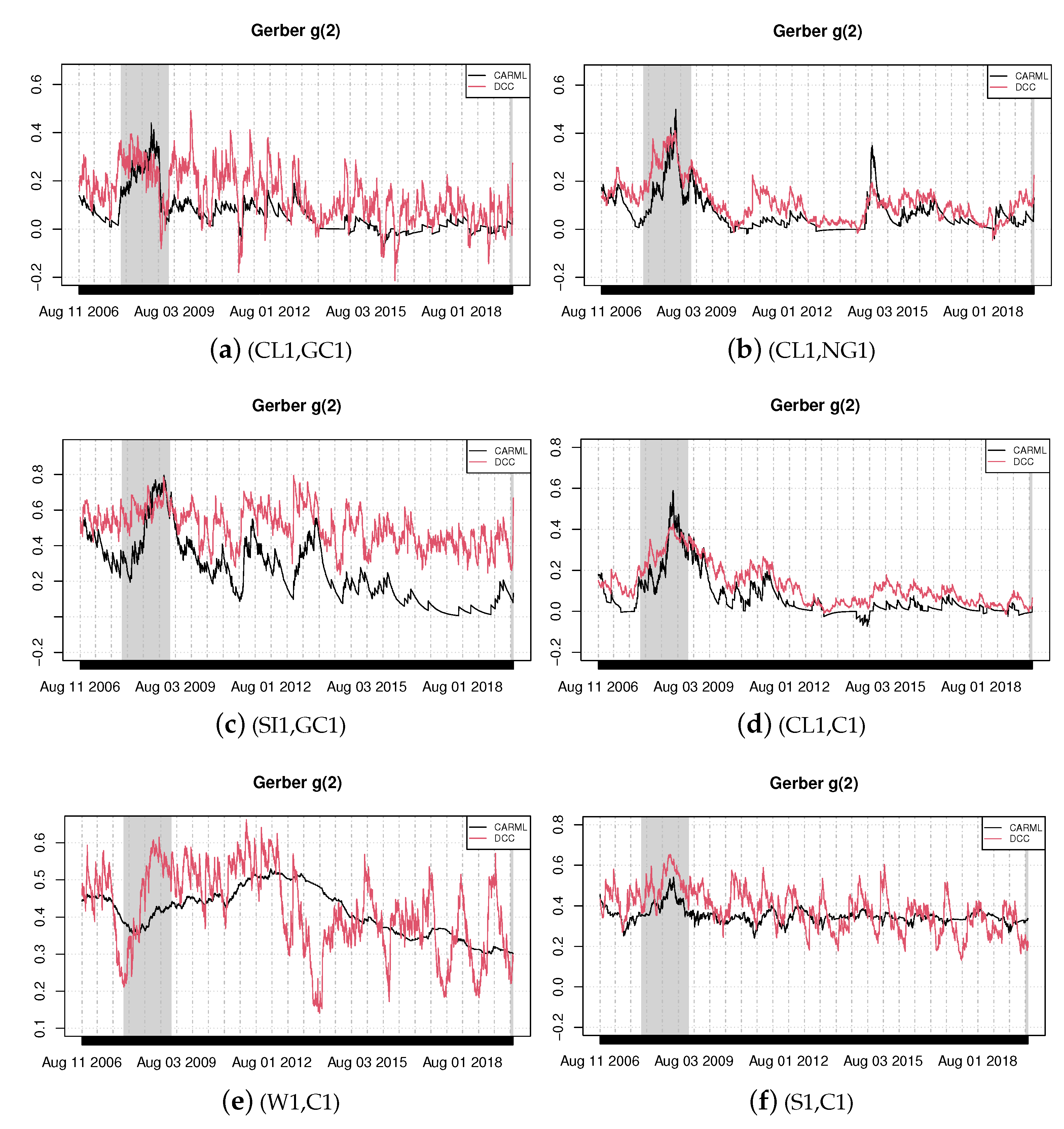
In this section, we estimate the CARML model in its reduced form, Equation (5), and the DCC model for six selected pairs of commodity returns using the whole sample of 3500 observations. Based on the estimated parameters, it is then possible to obtain a time-varying version of probabilities appearing in Equation (2) or Equation (3). For instance, in the case of the CARML model, we use Equation (8) with the estimated parameters and then Equation (6) to recover the time-varying probabilities. In turn, these are used to obtain the time-varying Gerber statistic. We plot the resulting time-varying Gerber correlations of Equation (3) in Figure 1 and Figure 2.
The shaded areas in the graphs—i.e., the periods from December 2007 to June 2009 and from February 2020 to the end of the period of investigation—describe the recession phases identified by the National Bureau of Economic Research. We find evidence of a significant degree of joint movements in our commodities and document that co-movements vary over time. Figure 1 visually shows the changing patterns of co-movements on a daily basis and the significant amount of correlation pervasiveness in commodity returns, with some degree of heterogeneity. Sharp co-movements are detected for the pairs silver–gold (SI1,GC1), wheat–corn (W1,C1) and crude oil–gold (CL1,GC1).
The high co-movements between silver and gold is due to their characteristics of hedging commodities [25,26]. The study by Jaffe [27] is one of the first analyses to empirically investigate the linkages between these two precious metals from 1971 to 1987. The pair was found to have a high correlation of 0.744. Erb and Harvey [28], using data between December 1982 and May 2004, showed that silver has very low correlation with other major commodities, except gold (0.66). Our findings, based on the robust measure we consider, corroborate previous studies and suggest that, since the two precious metals display high correlation, the inclusion of both commodities in the same portfolio would be redundant from an investment perspective. An interesting result is for the pair gold and copper (not reported graphically). There is a very low positive correlation between the two commodities during the global downturn of 2007–2008, while their correlation significantly rises during normal times. This finding reflects the fact that the yellow precious metal is produced, in the great majority, for investment purposes, while the red metal is destined almost entirely for industrial usage. Hence, copper prices and returns tend to increase when economies are strong and growing, simply because there is a greater global demand [29]. Conversely, gold prices and returns would rise when economies are weak, due to a risk aversion channel.
CARML and DCC models deliver similar results for the pairs crude oil–natural gas (CL1,NG1) and for crude oil–corn (CL1,C1). The joint return dynamics between crude oil and corn increased during the worldwide financial crisis. The rise in co-movements can be explained by the fact that an increase in oil prices generates contemporaneous upsurges in the price of other commodities, such as foodstuffs, via both the cost effect on the energy intensive agriculture sector and the substitution effect due to the increasing biofuel production which utilizes corn and soybeans [30]. As an energy-intensive sector, agriculture is traditionally linked to the energy industry through its input channels. While fuel and electricity are used directly in agricultural production, fertilizers and pesticides represent the two most prominent indirect energy inputs. Through these energy input channels, higher energy prices increase the cost of producing and transporting agricultural commodities.
The case of crude oil–gold (CL1,GC1) is interesting. Specifically, during critical economic and financial phases, gold is confirmed to be a ‘safe haven’ given that the common movements between the two commodities fall significantly during the recession phases (both during the period of the global financial crash and the period of sovereign crisis).
The pair soybean–corn (S1,C1) exhibits relatively high co-movements throughout the sample period. A possible reason for the strong common movements between the two commodities could be the demand for biofuels, since corn and soybean are the main crops that are used in the production of biofuels (biodiesel and ethanol) and are good substitutes.
The result further suggests that spikes in co-movements were more marked during the global financial crisis than in other periods. It also indicates that the joint return dynamics among energy, agricultural and metal commodities is always positive (excluding very few negative relations between oil and natural gas). These positive co-movements point to a reduced possibility of diversification across commodities in the short-run.
Finally, DCC models provide more volatile Gerber estimates than CARML models owing to the fact that they do not directly produce the probabilities needed for the Gerber statistic. DCC models indeed focus on the dynamics of the conditional correlation matrix and the probabilities are subsequently obtained via the integrals reported in Section 2.1.3. For CARML models, instead, the (logit transforms of) the required probabilities are directly modeled via the recursions described by Equation (4) or (5).
3.3. Out-of-Sample Analysis
To assess the out-of-sample forecasting performances of the considered models, we estimate them recursively. We use a moving window of length 1000 and end up with forecasts for the probabilities appearing in the Gerber correlations. We consider again the reduced form of CARML models, Equation (5). We compare the forecasting accuracy of different models using the Brier Scores defined as:
where represents the forecast obtained using model (conditional on the information up to ) and is the time t indicator associated to the region . For instance, when the investigated commodity returns are and , the indicator variables for the regions and are
The Brier score is a tool commonly used to evaluate probability forecasts (see, e.g., [19,31]). Since the expected value of the score is lowest for the true probability, the Brier score represents a proper scoring rule [32]. We compare the estimated models with the reference model (HS) using the Brier skill score defined as
Models that present a Brier skill score larger than zero have a superior forecasting accuracy compared to the reference model (historical simulation). Brier skill scores can also be used to compare the three alternative models considered in the present study as models with larger Brier skill scores are more accurate.
The Brier skill scores for the selected pairs of commodities are reported in Table 3. The results indicate that CARML models perform better in term of forecasting power when the thresholds are half the volatility. DCC models are more suitable when forecasting extreme commodity returns for energy and metals. Moreover, CARML models have higher forecasting power for agricultural commodities in the case in which the thresholds are set equal to the 90% quantiles. In all cases, CARML and DCC are more accurate than filtered historical simulation models. Table 4 instead refers to all 91 pairs of commodities we can form. In the table, we provide the number of pairs (and frequency, i.e., the number divided by 91) for which a model has a positive Brier skill score. In the table, we also give the number (and frequency) of pairs for which a given method presents a Brier skill score larger than an alternative model. The results confirm that both the CARML and DCC models outperform FHS. CARML models perform better than DCC models when the threshold is half the unconditional volatility, whereas the opposite is true when the threshold is set equal to the 90% quantile. From the analysis of all the possible pairs of commodities, we notice that CARML models tend to be more accurate when both commodities are of the agricultural type, while DCC models are more accurate when both commodities are energy products or metals.
4. Conclusions
The present study examined the co-movement of price returns for a broad spectrum of commodities for the years 2006–2020. Common movements across agricultural, energy and metal prices returns are a concern for consumers, producers, traders, investors and governments since any shock occurring to a specific commodity can easily propagate to the other commodities causing disruptive joint events. The issue of co-movement was addressed using a time-varying Gerber correlation and a set of models comprising historical simulation, filter historical simulation, DCC and CARML models. The findings reveal that there is evidence of co-movements across commodity returns and these co-movements change over time. The correlation appears more noticeable for the pairs wheat–corn, silver–gold, gold–oil and corn–soybeans. Commodity co-movements tend to rise during extreme market distress. On the basis of the Brier scores, CARML and DCC models show stronger forecasting power than the benchmark method (HS) irrespective of the choice of the thresholds. However, CARML models show higher forecasting accuracy for agricultural commodities, while DCC models are more accurate for energy products and metals. The reason can be linked to the ability of GARCH family models to better capture heteroskedasticity in the series, a feature that is more pronounced for energy and metals than agricultural products. Our results are important for financial market participants and portfolio managers in particular for building an optimal portfolio and forecasting joint futures commodity returns. For instance, the inclusion of gold and silver in the same portfolio would be redundant from an investment perspective given their high Gerber correlation. This research could be extended to stock markets or used to analyze the co-movement among spot and futures markets.
Author Contributions
Conceptualization, B.A., A.L. and P.T.; methodology, A.L.; software, A.L.; validation, B.A.; formal analysis, B.A.; investigation, B.A. and A.L.; data curation, B.A. and A.L.; visualization, A.L.; writing—original draft preparation, B.A.; and writing—review and editing, B.A., A.L. and P.T. All authors have read and agreed to the published version of the manuscript.
Funding
This research received no external funding.
Institutional Review Board Statement
Not applicable.
Informed Consent Statement
Not applicable.
Data Availability Statement
Data sharing not applicable.
Acknowledgments
We are grateful to the Editor, Michał Rubaszek, and two anonymous referees for very useful comments and suggestions which have helped to improve the manuscript. The usual disclaimer applies. We benefited from discussions with Lynda Khalaf and Debora Loccisano.
Conflicts of Interest
The authors declare no conflict of interest.
References
- Ali, S.; Bouri, E.; Czudaj, R.L.; Shahzad, S.J.H. Revisiting the valuable roles of commodities for international stock markets. Resour. Policy 2020, 66, 101603. [Google Scholar] [CrossRef]
- Hamilton, J.D.; Wu, J.C. Effect Of Index-Fund Investing On Commodity Futures Prices. Int. Econ. Rev. 2015, 56, 187–205. [Google Scholar] [CrossRef] [Green Version]
- Henderson, B.J.; Pearson, N.D.; Wang, L. New Evidence on the Financialization of Commodity Markets. Rev. Financ. Stud. 2015, 28, 1285–1311. [Google Scholar] [CrossRef] [Green Version]
- Cheng, I.H.; Xiong, W. Financialization of Commodity Markets. Annu. Rev. Financ. Econ. 2014, 6, 419–441. [Google Scholar] [CrossRef] [Green Version]
- Tang, K.; Xiong, W. Index Investment and the Financialization of Commodities. Financ. Anal. J. 2012, 68, 54–74. [Google Scholar] [CrossRef]
- Algieri, B. Fast & furious: Do psychological and legal factors affect commodity price volatility? World Econ. 2021, 44, 980–1017. [Google Scholar] [CrossRef]
- Yuan, X.; Tang, J.; Wong, W.K.; Sriboonchitta, S. Modeling Co-Movement among Different Agricultural Commodity Markets: A Copula-GARCH Approach. Sustainability 2020, 12, 393. [Google Scholar] [CrossRef] [Green Version]
- Mensi, W.; Beljid, M.; Boubaker, A.; Managi, S. Correlations and volatility spillovers across commodity and stock markets: Linking energies, food, and gold. Econ. Model. 2013, 32, 15–22. [Google Scholar] [CrossRef] [Green Version]
- Baur, D.G. What Is Co-Movement? Technical Report 20759; EUR European Commission Joint Research Centre: Ispra, Italy, 2003. [Google Scholar]
- Tadasse, G.; Algieri, B.; Kalkuhl, M.; von Braun, J. Drivers and Triggers of International Food Price Spikes and Volatility. In Food Price Volatility and Its Implications for Food Security and Policy; Kalkuhl, M., von Braun, J., Torero, M., Eds.; Springer International Publishing: Cham, Switzerland, 2016; pp. 59–82. [Google Scholar] [CrossRef] [Green Version]
- Algieri, A.; Morrone, P.; Bova, S. Techno-Economic Analysis of Biofuel, Solar and Wind Multi-Source Small-Scale CHP Systems. Energies 2020, 13, 3002. [Google Scholar] [CrossRef]
- Brück, T.; d’Errico, M. Reprint of: Food security and violent conflict: Introduction to the special issue. World Dev. 2019, 119, 145–149. [Google Scholar] [CrossRef]
- Bellemare, M.F. Rising Food Prices, Food Price Volatility, and Social Unrest. Am. J. Agric. Econ. 2015, 97, 1–21. [Google Scholar] [CrossRef] [Green Version]
- Byrne, J.P.; Fazio, G.; Fiess, N. Primary commodity prices: Co-movements, common factors and fundamentals. J. Dev. Econ. 2013, 101, 16–26. [Google Scholar] [CrossRef] [Green Version]
- Umar, Z.; Zaremba, A.; Olson, D. Seven centuries of commodity co-movement: A wavelet analysis approach. Appl. Econ. Lett. 2020, 1–5. [Google Scholar] [CrossRef]
- Gerber, S.; Javid, B.; Markowitz, H.; Sargen, P.; Starer, D. The Gerber Statistic: A Robust Measure of Correlation; Technical Report; Hudson Bay Capital Management: New York, NY, USA, 2019. [Google Scholar]
- Zaremba, A.; Umar, Z.; Mikutowski, M. Commodity financialisation and price co-movement: Lessons from two centuries of evidence. Financ. Res. Lett. 2021, 38, 101492. [Google Scholar] [CrossRef]
- Harvey, A.C. Forecasting, Structural Time Series Models and the Kalman Filter; Cambridge University Press: Cambridge, UK, 1990. [Google Scholar]
- Taylor, J.W. Probabilistic forecasting of wind power ramp events using autoregressive logit models. Eur. J. Oper. Res. 2017, 259, 703–712. [Google Scholar] [CrossRef]
- Engle, R. Dynamic Conditional Correlation: A Simple Class of Multivariate Generalized Autoregressive Conditional Heteroskedasticity Models. J. Bus. Econ. Stat. 2002, 20, 339–350. [Google Scholar] [CrossRef]
- Dufour, J.M.; Valéry, P. Exact and asymptotic tests for possibly non-regular hypotheses on stochastic volatility models. J. Econ. 2009, 150, 193–206. [Google Scholar] [CrossRef] [Green Version]
- Luger, R. Finite-sample bootstrap inference in GARCH models with heavy-tailed innovations. Comput. Stat. Data Anal. 2012, 56, 3198–3211. [Google Scholar] [CrossRef]
- Abdelkhalek, T.; Dufour, J.M. Statistical Inference for Computable General Equilibrium Models, with Application to A Model of the Moroccan Economy. Rev. Econ. Stat. 1998, 80, 520–534. [Google Scholar] [CrossRef] [Green Version]
- Engle, R.F. Autoregressive Conditional Heteroscedasticity with Estimates of the Variance of United Kingdom Inflation. Econometrica 1982, 50, 987–1007. [Google Scholar] [CrossRef]
- Vigne, S.A.; Lucey, B.M.; O’Connor, F.A.; Yarovaya, L. The financial economics of white precious metals—A survey. Int. Rev. Financ. Anal. 2017, 52, 292–308. [Google Scholar] [CrossRef] [Green Version]
- O’Connor, F.A.; Lucey, B.M.; Batten, J.A.; Baur, D.G. The financial economics of gold — A survey. Int. Rev. Financ. Anal. 2015, 41, 186–205. [Google Scholar] [CrossRef]
- Jaffe, J.F. Gold and Gold Stocks as Investments for Institutional Portfolios. Financ. Anal. J. 1989, 45, 53–59. [Google Scholar] [CrossRef]
- Erb, C.B.; Harvey, C.R. The Strategic and Tactical Value of Commodity Futures. Financ. Anal. J. 2006, 62, 69–97. [Google Scholar] [CrossRef]
- Caldara, D.; Cavallo, M.; Iacoviello, M. Oil price elasticities and oil price fluctuations. J. Monet. Econ. 2019, 103, 1–20. [Google Scholar] [CrossRef] [Green Version]
- Algieri, B.; Leccadito, A. Extreme price moves: An INGARCH approach to model coexceedances in commodity markets. Eur. Rev. Agric. Econ. 2020, jbaa030. [Google Scholar] [CrossRef]
- Taylor, J.W.; Yu, K. Using auto-regressive logit models to forecast the exceedance probability for financial risk management. J. R. Stat. Soc. Ser. (Stat. Soc.) 2016, 179, 1069–1092. [Google Scholar] [CrossRef] [Green Version]
- Gneiting, T.; Balabdaoui, F.; Raftery, A.E. Probabilistic forecasts, calibration and sharpness. J. R. Stat. Soc. Ser. (Stat. Methodol.) 2007, 69, 243–268. [Google Scholar] [CrossRef] [Green Version]
Figure 1.
Time-varying Gerber correlations, Equation (3). Thresholds are and where and are the (unconditional) return volatilities.
Figure 1.
Time-varying Gerber correlations, Equation (3). Thresholds are and where and are the (unconditional) return volatilities.
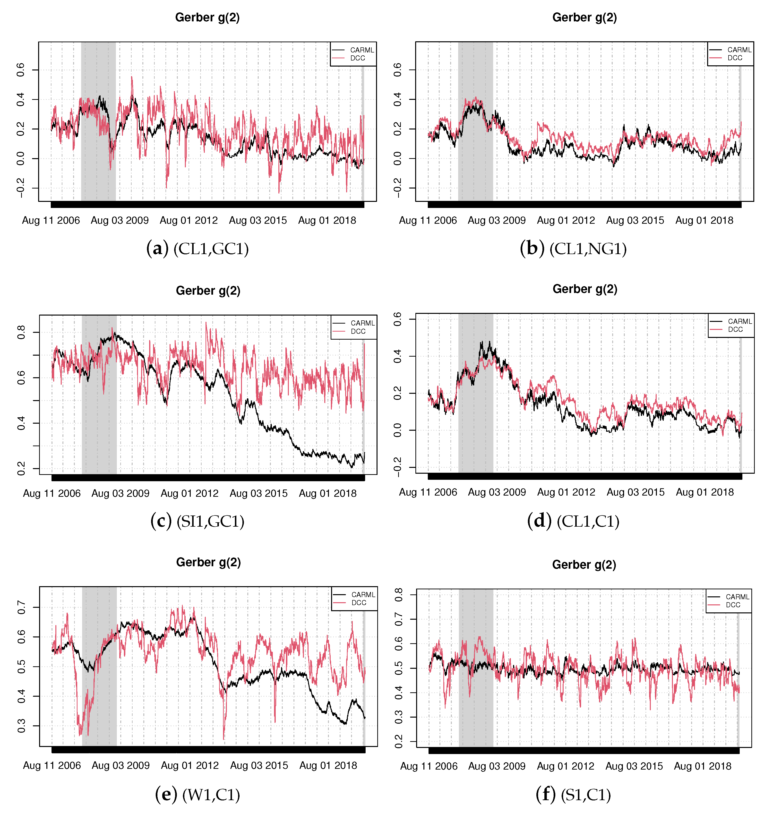
Figure 2.
Time-varying Gerber correlations, Equation (3). Thresholds are and where and are the (unconditional) quantiles of the returns.
Figure 2.
Time-varying Gerber correlations, Equation (3). Thresholds are and where and are the (unconditional) quantiles of the returns.

Table 1.
Commodity futures (Bloomberg Tickers).
| Selected Commodities | |
|---|---|
| Ticker | Description |
| C1 Comdty | Generic 1st Corn No. 2 Yellow futures, US$ |
| S1 Comdty | Generic 1st Soybean No. 2 Yellow futures, US$ |
| W1 Comdty | Generic 1st Wheat futures, US$ |
| CL1 Comdty | WTI crude oil |
| NG1 Comdty | Natural Gas |
| GC1 Comdty | Gold |
| SI1 Comdty | Silver |
| Remaining Agricultural Commodities | |
| Ticker | Description |
| KC1 Comdty | Generic 1st Coffee futures contract |
| SB1 Comdty | Generic 1st Sugar No. 11 (raw) futures |
| RR1 Comdty | Generic 1st Rice futures |
| CC1 Comdty | Generic 1st Cocoa |
| Remaining Energy Commodities | |
| Ticker | Description |
| CO1 Comdty | Brent Oil |
| HO1 Comdty | Heating oil |
| Remaining Metals | |
| Ticker | Description |
| HG1 Comdty | Copper |
Table 2.
Descriptive statistics for the log-returns of commodities futures.
| Selected Commodities | |||||||
|---|---|---|---|---|---|---|---|
| C1 | S1 | W1 | CL1 | NG1 | GC1 | SI1 | |
| Min. | −0.081 | −0.073 | −0.098 | −0.119 | −0.186 | −0.098 | −0.195 |
| 1st Qu | −0.008 | −0.007 | −0.010 | −0.010 | −0.015 | −0.004 | −0.007 |
| Median | 0.000 | 0.000 | 0.000 | 0.000 | −0.001 | 0.001 | 0.001 |
| Mean | 0.000 | 0.000 | 0.000 | 0.000 | 0.000 | 0.000 | 0.000 |
| 3rd Qu | 0.009 | 0.007 | 0.010 | 0.010 | 0.014 | 0.006 | 0.009 |
| Max. | 0.086 | 0.065 | 0.086 | 0.135 | 0.166 | 0.086 | 0.124 |
| Std. Dev. | 0.016 | 0.013 | 0.018 | 0.020 | 0.026 | 0.011 | 0.019 |
| Skewness | −0.043 | −0.252 | 0.034 | 0.030 | 0.141 | −0.475 | −0.916 |
| Kurtosis | 5.411 | 5.818 | 5.033 | 7.013 | 5.862 | 10.335 | 11.132 |
| JB stat. | 1214.252 | 1710.147 | 863.537 | 3360.445 | 1726.199 | 11,407.754 | 14,491.883 |
| JB pval. | 0 | 0 | 0 | 0 | 0 | 0 | 0 |
| Q1 | 652.816 | 667.872 | 577.179 | 765.575 | 796.927 | 777.274 | 846.418 |
| Q5 | 961.155 | 1241.034 | 842.120 | 1436.187 | 1068.713 | 935.768 | 951.451 |
| Q1 pval. | 0 | 0 | 0 | 0 | 0 | 0 | 0 |
| Q5 pval. | 0 | 0 | 0 | 0 | 0 | 0 | 0 |
| LM1 | 5073.130 | 5761.032 | 4919.449 | 6467.057 | 4966.216 | 8230.659 | 7457.130 |
| LM5 | 1567.114 | 1661.710 | 1531.263 | 1845.515 | 1577.667 | 2625.688 | 2431.796 |
| LM1 pval. | 0 | 0 | 0 | 0 | 0 | 0 | 0 |
| LM5 pval. | 0 | 0 | 0 | 0 | 0 | 0 | 0 |
| Remaining Agricultural Commodities | Remaining Energy Commodities | Remaining Metals | |||||
| KC1 | SB1 | RR1 | CC1 | CO1 | HO1 | HG1 | |
| Min. | −0.111 | −0.124 | −0.062 | −0.096 | −0.103 | −0.098 | −0.116 |
| 1st Qu | −0.010 | −0.009 | −0.007 | −0.009 | −0.009 | −0.009 | −0.007 |
| Median | 0.000 | 0.000 | 0.000 | 0.000 | 0.000 | 0.000 | 0.000 |
| Mean | 0.000 | 0.000 | 0.000 | 0.000 | 0.000 | 0.000 | 0.000 |
| 3rd Qu | 0.010 | 0.009 | 0.007 | 0.009 | 0.009 | 0.009 | 0.008 |
| Max. | 0.110 | 0.087 | 0.054 | 0.082 | 0.133 | 0.103 | 0.117 |
| Std. Dev. | 0.017 | 0.018 | 0.012 | 0.016 | 0.019 | 0.017 | 0.016 |
| Skewness | 0.047 | -0.313 | −0.003 | −0.210 | 0.047 | 0.064 | −0.043 |
| Kurtosis | 5.104 | 6.087 | 4.298 | 5.472 | 7.267 | 6.115 | 7.703 |
| JB stat. | 925.756 | 2071.051 | 351.917 | 1312.606 | 3800.539 | 2028.498 | 4615.341 |
| JB pval. | 0 | 0 | 0 | 0 | 0 | 0 | 0 |
| Q1 | 519.798 | 679.805 | 566.418 | 393.100 | 790.971 | 646.284 | 930.245 |
| Q5 | 578.844 | 779.116 | 691.245 | 462.829 | 1514.100 | 1230.272 | 1894.352 |
| Q1 pval. | 0 | 0 | 0 | 0 | 0 | 0 | 0 |
| Q5 pval. | 0 | 0 | 0 | 0 | 0 | 0 | 0 |
| LM1 | 5203.071 | 5511.624 | 3811.809 | 6051.277 | 6428.943 | 5983.694 | 6486.196 |
| LM5 | 1683.965 | 1809.333 | 1238.506 | 1962.049 | 1828.758 | 1717.633 | 1737.276 |
| LM1 pval. | 0 | 0 | 0 | 0 | 0 | 0 | 0 |
| LM5 pval. | 0 | 0 | 0 | 0 | 0 | 0 | 0 |
Note: ‘JB stat.’ and ‘JB pval.’ denote the Jarque–Bera test statistic and p-value, respectively. ‘Q1’ and ‘Q5’ are the Ljung–Box test statistics (with 1 and 5 lags) calculated on squared returns and ‘Q1 pval.’, ‘Q5 pval.’ are their p-values. ‘LM1’ and ‘LM5’ are the test statistics (with 1 and 5 lags) for Engle’s ARCH test and ‘LM1 pval.’ and ‘LM5 pval.’ are their p-values.
Table 3.
Brier skill scores for the selected pairs of commodities.
| and | |||
|---|---|---|---|
| (GC1,CL1) | 3.245 | 1.229 | 1.152 |
| (CL1,NG1) | 3.534 | 1.805 | 0.870 |
| (GC1,SI1) | 0.461 | −0.512 | −0.270 |
| (CL1,C1) | 3.689 | 1.979 | 1.120 |
| (C1,W1) | 2.325 | 0.744 | −0.415 |
| (C1,S1) | 0.220 | 0.294 | −3.201 |
| and | |||
| (GC1,CL1) | 1.553 | 2.827 | 1.149 |
| (CL1,NG1) | 0.489 | 2.885 | −0.034 |
| (GC1,SI1) | 1.818 | 0.064 | −0.125 |
| (CL1,C1) | 3.418 | 4.242 | −0.373 |
| (C1,W1) | 2.833 | 1.425 | −0.079 |
| (C1,S1) | 0.526 | 0.873 | −2.625 |
Note: The thresholds correspond to half the unconditional volatilities or to the 90% quantiles of the returns. The model with the best score is in bold.
Table 4.
Brier skill scores for all the pairs of commodities.
| and | |||
|---|---|---|---|
| NUM | 89 | 90 | 84 |
| FREQ | 0.978 | 0.989 | 0.923 |
| and | |||
| NUM | 88 | 91 | 73 |
| FREQ | 0.967 | 1.000 | 0.802 |
| and | |||
| NUM | 89 | 91 | 51 |
| FREQ | 0.978 | 1.000 | 0.560 |
| and | |||
| NUM | 89 | 91 | 51 |
| FREQ | 0.978 | 1.000 | 0.560 |
Note: The thresholds correspond to half the unconditional volatilities or to the 90% quantiles of the returns.
Table 5.
Brier skill scores for the selected pairs of commodities.
| and | |||
|---|---|---|---|
| (GC1,CL1) | 3.280 | 2.568 | 2.125 |
| (CL1,NG1) | 3.489 | 2.885 | 0.897 |
| (GC1,SI1) | 1.270 | 0.064 | 0.970 |
| (CL1,C1) | 3.418 | 4.242 | 1.373 |
| (C1,W1) | 2.833 | 1.425 | 1.079 |
| (C1,S1) | 1.896 | 2.843 | 0.297 |
| and | |||
| (GC1,CL1) | 1.297 | 2.272 | 0.791 |
| (CL1,NG1) | 0.386 | 2.269 | −0.123 |
| (GC1,SI1) | 1.192 | 0.164 | −0.070 |
| (CL1,C1) | 2.942 | 3.722 | −0.373 |
| (C1,W1) | 2.138 | 2.675 | −0.079 |
| (C1,S1) | 0.397 | 0.973 | 0.059 |
Note: The thresholds correspond to the 85% quantiles or to the 95% quantiles of the returns. The model with the best score is in bold.
Table 6.
Brier skill scores for all pairs of commodities.
| and | |||
|---|---|---|---|
| NUM | 90 | 90 | 87 |
| FREQ | 0.989 | 0.989 | 0.956 |
| and | |||
| NUM | 87 | 91 | 89 |
| FREQ | 0.956 | 1.000 | 0.978 |
| and | |||
| NUM | 86 | 91 | 63 |
| FREQ | 0.945 | 1.000 | 0.692 |
| and | |||
| NUM | 54 | 91 | 91 |
| FREQ | 0.593 | 1.000 | 1.000 |
Note: The thresholds correspond to the 85% quantiles or to the 95% quantiles of the returns.
Publisher’s Note: MDPI stays neutral with regard to jurisdictional claims in published maps and institutional affiliations. |
© 2021 by the authors. Licensee MDPI, Basel, Switzerland. This article is an open access article distributed under the terms and conditions of the Creative Commons Attribution (CC BY) license (https://creativecommons.org/licenses/by/4.0/).
Share and Cite
MDPI and ACS Style
Algieri, B.; Leccadito, A.; Toscano, P. A Time-Varying Gerber Statistic: Application of a Novel Correlation Metric to Commodity Price Co-Movements. Forecasting 2021, 3, 339-354. https://0-doi-org.brum.beds.ac.uk/10.3390/forecast3020022
AMA Style
Algieri B, Leccadito A, Toscano P. A Time-Varying Gerber Statistic: Application of a Novel Correlation Metric to Commodity Price Co-Movements. Forecasting. 2021; 3(2):339-354. https://0-doi-org.brum.beds.ac.uk/10.3390/forecast3020022
Chicago/Turabian StyleAlgieri, Bernardina, Arturo Leccadito, and Pietro Toscano. 2021. "A Time-Varying Gerber Statistic: Application of a Novel Correlation Metric to Commodity Price Co-Movements" Forecasting 3, no. 2: 339-354. https://0-doi-org.brum.beds.ac.uk/10.3390/forecast3020022