Article

Forecasting Internal Migration in Russia Using Google Trends: Evidence from Moscow and Saint Petersburg

by
Dean Fantazzini
1,*,
Julia Pushchelenko
2,
Alexey Mironenkov
1 and
Alexey Kurbatskii
1
1
Moscow School of Economics, Moscow State University, 119234 Moscow, Russia
2
Higher School of Economics, 101000 Moscow, Russia
*
Author to whom correspondence should be addressed.
Submission received: 1 September 2021 / Revised: 22 October 2021 / Accepted: 23 October 2021 / Published: 28 October 2021

Abstract

:
This paper examines the suitability of Google Trends data for the modeling and forecasting of interregional migration in Russia. Monthly migration data, search volume data, and macro variables are used with a set of univariate and multivariate models to study the migration data of the two Russian cities with the largest migration inflows: Moscow and Saint Petersburg. The empirical analysis does not provide evidence that the more people search online, the more likely they are to relocate to other regions. However, the inclusion of Google Trends data in a model improves the forecasting of the migration flows, because the forecasting errors are lower for models with internet search data than for models without them. These results also hold after a set of robustness checks that consider multivariate models able to deal with potential parameter instability and with a large number of regressors.

1. Introduction

Google Trends (GT) is an online service launched in 2008, which provides an index that reflects the relative popularity of a particular keyword (or a topic) by calculating the share of users’ searches for this keyword among the total Google searches. This tool has been used in various fields of research, including IT, communications, medicine, health, business, and economics; see the large [1] for a detailed review.
One of the latest advances in migration research proposes the inclusion of Google Trends data to forecast migration flows. In this regard, Böhme et al. [2] stated that people acquire information about migration opportunities online before deciding to emigrate. Therefore, the online demand for information can serve as a proxy for future changes in the number of migrants; changes in online search intensity for specific keywords related to migration can indicate an increase in the demand for migration and, thus, can help to predict migration flows. We remark that there is an increasing literature that shows that Google-based models significantly outperform most of their competitors in several economic and financial applications; see [3,4,5,6,7,8]. Jun et al. [7] provide a useful review of the research using Google Trends in a wide range of areas, including IT, communications, medicine, health, business, and economics.
In this perspective, we propose to use online search data for forecasting the monthly aggregate migration inflows into Russian regions from all other regions. We justify this choice because the administrative burden of registering in a new region is nontrivial and takes some time (See the official detailed requirements in Russian: https://www.gosuslugi.ru/situation/residential_property/registration_of_citizens, and http://www.consultant.ru/document/cons_doc_LAW_7271/2ab816e63f6cf336e7c992753d7a3c5c9a517997, accessed on 1 October 2021), and searching the web for information is one of the main strategies a potential immigrant can adopt. Moreover, given that the most important requirement to register in a new region is having a place to stay, searching the web is needed to look for a house/flat to buy or rent. Furthermore, the official statistics on monthly migration are published with a lag of (usually) 6 months, and are not available when a regional government starts planning the social and labor policies in that region. Instead, internet search data are available on a weekly and monthly basis, and they can help to identify in advance the number of people that have an intention to move. Therefore, internet data may provide precise migration forecasts long before the release of official statistics, thus giving the regional governments more time and better information to plan their local policies. In this regard, [9,10] recently highlighted that the lack of reliable hard data limits the possibility of policymakers making informed decisions, and they suggested employing auxiliary data from social media such as Google Trends. Our proposal in this paper goes in this direction (In August 2021, using the simple average of the market shares for search engines provided by the analytics services Yandex-Radar and StatCounter, Yandex was the top search engine in Russia with a share of 51%, while Google had a share of 45%. Unfortunately, Yandex provides only the last 24 months of search data, thus making any statistical analysis with monthly data unfeasible. It is for this reason that we used Google search data in place of Yandex data).
We use monthly migration data, search volume data, and macro variables for the 2009–2018 time period to analyze how these variables affect migration inflows for the two Russian cities with the largest migration inflows: Moscow and Saint Petersburg (The focus of this paper is on legal migrants. Of course, we are aware that there are a large number of illegal migrants in these two cities: unfortunately, the estimates of these immigrants vary widely, and are not always available (see e.g., https://ru.wikipedia.org/wiki/%D0%93%D0%B0%D1%81%D1%82%D0%B0%D1%80%D0%B1%D0%B0%D0%B9%D1%82%D0%B5%D1%80%D1%8B_%D0%B2_%D0%A0%D0%BE%D1%81%D1%81%D0%B8%D0%B8 for a summary, accessed on 1 October 2021), so that it is difficult—if not impossible—to build a reliable model using these estimates. However, we are confident that both legal and illegal migration share the same temporal dynamics, as was particularly evident during the COVID-19 pandemic in 2020; see e.g., https://en.wikipedia.org/wiki/Immigration_to_Russia, accessed on 1 October 2021). We consider both short- and long-term forecasts, because in real life the regional government has to plan social and labor policy for at least a year in advance. ARIMA-class models are used to make one-step-ahead forecasts, while multivariate models are used for recursive long-term forecasting up to 24 months ahead.
The empirical analysis does not provide evidence that the more people search online, the more they relocate to other regions. Instead, we find that a one-time shock in internet search queries results in a negative migration inflow after approximately five months. However, the inclusion of Google Trends data in a model does improve the forecasting of the migration inflows, because the forecasting errors are lower for models with internet search data than for models without them. These results also hold after a set of robustness checks that consider multivariate models able to deal with potential parameter instability and with a large number of regressors—potentially larger than the number of observations.
The use of Google search data represents an important leading indicator for migration dynamics, which can complement other instruments, such as data from other social media and telecommunications data, as recently discussed in [11]. The increasing availability to policymakers of a wide array of leading indicators can be useful to improve both the development and the implementation of migration policies (The research in this paper received financial support from a grant from the Russian Science Foundation. The policymakers’ interest in using such instruments was indirectly confirmed by the request made to us by the grant reviewers to focus specifically on the possibility of forecasting migration flows using Google search data).
The rest of this paper is organized as follows: Section 2 briefly reviews the literature devoted to migration research with Google Trends and online data, while the methods proposed for forecasting the migration flows in Moscow and Saint Petersburg are discussed in Section 3. The empirical results are reported in Section 4, while Section 5 briefly concludes the paper. Robustness checks are discussed in the Appendix A, Appendix B and Appendix C.

2. Literature Review

2.1. Migration

The study of migration in Russia is based on different approaches. One of the oldest streams of migration research employed the spatial structure of data to explain migration flows between regions; see [12,13,14,15], to name but a few.
Another strand of literature focuses on time-series models, and mainly employs two types of models: ARIMA-class models and extrapolation of time series through the propagation of historical forecast errors, see [16] and references therein for a review. These models can also be extended using expert-based information through prior distributions and Bayesian methods. In this regard, [16] uses time-series models with and without expert opinions, and considers three types of model: ARIMA-class models, autoregressive distributed lag (ADL) models, and historical propagation of forecast errors. They found that ARMA models of low orders showed better performances with stationary data, whereas ADL models worked better with non-stationary data.
In the past decade, there has been a large set of works that focused on the main factors affecting migration, including economic, institutional, and legal conditions, labor market performance measures, and numerous other factors; see e.g., [17,18,19,20,21,22,23,24,25,26]. We refer to [27] and [28] for an overview of this field of research.
There is also a smaller but increasing literature that uses social big data to measure migration dynamics and future patterns. These data come from social media, internet search services (A specific review of the literature dealing with internet search services is reported in Section 2.2), mobile phones, supermarket transaction data, and other sources. They can contain detailed information about their users, and can cover larger sets of the population than traditional data sources. Moreover, they can provide immigrants’ movements in real time and show the immigration trends even before the official statistics are published; see e.g., [29]. [30] inferred migration patterns using Twitter data, while [31] discovered the origins of immigrants from the language used in tweets. Skype ego networks (Ego-centric social networks -or ego-networks- map the interactions that take place between the social contacts of individual people) data can also be used to explain international migration patterns; see [32] for a detailed discussion. Furthermore, big data can be used to study the movements of individuals in times of crisis, as suggested by [33], who proposed to improve the response to disasters and outbreaks by tracking population movements with mobile phone network data. Sirbu et al. [11] provide a survey of this interesting new literature dealing with human migration and big data.
In the Russian literature, the focus has been on modeling interregional migration using econometric methods, moving from initial cross-sectional data, to panel data dealing with net migration rates, through to panel data models for interregional gross migration flows. Even though different datasets were used, the results of these studies are similar, and they highlight that the overall migration flow is low compared to other countries of similar size (such as the US or Canada); see [34] and references therein. Moreover, the main idea is that the Russian economy is in disequilibrium, and that the migration flows depend on economic fundamentals, such as the differences in the public service provisions, incomes, and unemployment rates between regions. Vakulenko et al. [35] and Korovkin et al. [36] provided additional insights by showing that the main determinants of interregional migration are factors that reflect the situation in the labor and residential markets in the region of arrival. Finally, recent works have employed time-series methods for modeling migration data, such as the study of Pavlovskij [37], who applied ARIMA models for the short-term forecasting of migration inflows and outflows in Russian regions.
We remark that a large proportion of the migrants searching for work in Moscow and Saint Petersburg are from the former Soviet republics. Following the fall of the Soviet Union, Russia became a major destination country for international migrants, with officially almost 12 million foreign-born residents in 2017 [38]. In the 1990s, most immigrants were ethnic Russians fleeing from the new post-Soviet republics, whereas the composition of migration flows changed in the 2000s to non-Russian labor migrants [39,40]. This shift was caused by two changes: more liberal policies to grant work permits to non-ethnic Russian citizens of the Commonwealth of Independent States (CIS), and the better performance of Russia’s economy compared to the other economies in the region; see [41] and references therein for a larger discussion. In this regard, we highlight that requirements for obtaining work permits have changed over time, both in policy and in implementation; see e.g., [42,43]. Moreover, several studies showed that most labor migrants from the CIS countries are illegal, due to government limits on the number of admitted migrants, complex procedures for obtaining legal status, and incentives for employers to hire undocumented migrants rather than follow those procedures; see [43,44]. This lack of legal status has stimulated a business in fake documents and an array of methods to avoid deportation by the authorities; see [45,46].
A large body of literature discusses how migrants from CIS countries learned of opportunities to migrate thanks to their connections with other migrants or family/friends in Russia (usually known as “migrant networks”); see [41] and references therein. Demintseva and Peshkova [47], Demintseva and Kashnitsky [48], and Demintseva [49] showed that social networking sites—such as Odnoklassniki.ru and VKontakte.ru—are among the most important means of communicating by foreign migrants, and they are actively used when looking for accommodation and work. Bedrina et al. [50] recently provided a detailed econometric analysis of Uzbek migration networks in Russia. Timoshkin [51] further analyzed the whole spectrum of digital migration networks, and suggested that the success of these digital platforms is due to the complexity of official interfaces to communicate with state information nodes (e.g., regulations, job descriptions, normative acts), which make them unsuitable for communicating at a proper level. As a consequence, Timoshkin [51] suggests that these “migrant” digital platforms—such as social media and other information webpages—have become an “instrument that compensates for the technological imperfection of the state information hubs”. Abashin [52], Chudinovskikh and Denisenko [53], and Denisenko et al. [54] provide large historical surveys and analyses of labor migration in the post-Soviet territories.

2.2. Google Trends and Its Applications in Migration Research

Ettredge et al. [55] were among the first to discuss web-based search data to predict macroeconomic statistics. Since then, the research scope has expanded to a variety of other applications thanks to the seminal paper by Choi and Varian [3], which proposed the use of Google Trends data in several fields, including automobile sales, travel planning, consumer confidence, and many others. Several central banks have analyzed the suitability of Google Trends for predicting economic fundamentals; see, for example, [56,57].
Google Trends data have been widely used in the fields of fertility, mortality, and migration. With regard to fertility, Billari et al. [58] found that online search queries could reveal the intention to have a child in the coming months and, as such, can be used to increase the forecasting power of traditional demographic models. Mortality research in developing countries has benefited from using mobile phone data that store information about causes of death across the country; see [59] for more details. As for migration, Qin and Zhu [60] studied the effects of an air pollution index on intentions to emigrate using an online search index on “emigration” via Baidu—the largest Chinese search engine; they found that severe air pollution in the short term may significantly increase people’s interest in emigration, but this effect varies across Chinese regions. Böhme et al. [2], as far as we know, were the first to analyze the potential of online search data for predicting migration flows; they built a large set of fixed-effects models for migration flows based on yearly migration data, Google Trends data from the origin countries, and several control variables, as suggested by [17]. This approach proved to be successful in providing real-time forecasts of current migration flows ahead of official statistics, and to improve the forecasting performances of conventional models of migration flow.

3. Materials and Methods

The goal of this paper was to verify whether Google Trends data can be useful for modeling and predicting internal migration in Russia. To this end, we performed an out-of-sample forecasting analysis using a set of time-series models; given that sufficiently long time-series data for migration in Russia have become available, time series analysis can now be used. Following [2,16,37], we used traditional ARIMA models with and without Google Trends to investigate the impact of this new data source for migration forecasting, as well as multivariate models for long-term forecasting. Moreover, as suggested by [61], for each class of models we considered both a “standard” model with variables in levels and a model using logarithms.
Before presenting the results of the empirical analysis, we briefly review the forecasting models that we used to predict the monthly migration data for the two Russian cities with the largest migration inflows: Moscow and Saint Petersburg.

3.1. Forecasting Methods

The out-of-sample forecasting analysis employed three classes of models: univariate time-series models and Google-augmented univariate time-series models for one-step-ahead forecasts, along with multivariate models for long-term forecasts. A brief description of each model is reported below.

3.1.1. Models for Short-Term Forecasts

The first class of models employed in our analysis is the class of autoregressive integrated moving average (ARIMA) models based on migration data only. A non-seasonal ARIMA (p,d,q) model can be represented as follows:
( 1 ϕ 1 L ϕ p L p ) ( Δ d y t μ ) = ( 1 + θ 1 L + + θ 1 L q ) ε t
where Δ d y t = ( 1 L ) d , µ is the mean of Δ d y t , and L is the usual lag operator. ARIMA models represent a standard benchmark in time-series analysis, and we refer to Hamilton [62] for more details. Following Keilman et al. [61], we considered models with variables in levels and in log-levels. In the case of seasonal data, a seasonal ARIMA (SARIMA) can be used:
( 1 Φ 1 L S Φ P L P S ) ( 1 ϕ 1 L ϕ p L p ) ( Δ d y t μ ) = ( 1 + Θ 1 L S + + Θ Q L Q S ) ( 1 + θ 1 L + + θ 1 L q ) ε t
which can be written compactly as ARIMA (p,d,q)(P,D,Q)[S]. Information criteria can be used to find the optimal number of lags for the autoregressive and moving average terms.
If we augment the previous class of models with Google search data, we obtain an autoregressive integrated moving average model with exogenous variables (ARIMA-X):
( 1 ϕ 1 L ϕ p L p ) ( Δ d y t μ ) = β x t 1 + ( 1 + θ 1 L + + θ 1 L q ) ε t
where xt−1 is the lagged Google search index at time t − 1, and β is a coefficient. Seasonal components may be added if needed.

3.1.2. Models for Long-Term Forecasts

We used vector autoregression (VAR) models and vector error correction (VEC) models to consider the potential effects of both macroeconomic and search variables on migration flows, and to build long-term forecasts. A general VAR model of order p denoted as VAR(p) is given by:
Y t = Φ 0 + i = 1 p Φ i Y t i + u t , u t W N ( 0 , Σ )
where Yt is the (n × 1) vector of endogenous variables, Φ0 is an intercept vector, and Φi are the usual coefficient matrices with i = 1, …, p. As the primary focus of this paper is forecasting, the VAR(p) model is estimated in levels, and no differencing is applied to non-stationary data. The lag order p of the VAR is selected using the Akaike and Bayesian information criteria. The estimated VAR model is then analyzed by reporting its impulse response functions (IRFs) and its forecast error variance decomposition (FEVD); see [63] (Chapters 2–5) for more details.
We decided to use a simple VAR(p) in levels following the suggestion by Gospodinov et al. [63], who stated that the “unrestricted VAR in levels appears to be the most robust specification when there is uncertainty about the magnitude of the largest roots and the co-movement between the variables”. This is definitely our case, given the moderate size of our dataset (120 observations); in this regard, we want to remark that Elliott [64] was the first to show that co-integration methods may deliver large size distortions in the case of systems with near unit roots. Similar distortions can take place when using sequential modeling and specification procedures based on pretests for unit roots. Moreover, it is possible to show that the estimates of the impulse responses using VAR in levels remain asymptotically valid under weak conditions, even when the underlying process contains a unit root (or is possibly co-integrated with other variables), and the same holds true for forecast error variance decompositions at any finite horizon; see Inoue and Kilian [65] for more details. Instead, differencing the variables when they are stationary causes these estimates to be inconsistent and inference to be invalid. However, for sake of generality and interest, we also considered a VEC model following the standard sequential specification procedure based on pretests for unit roots and co-integration; see [63] (Chapters 6–8), for more details.
Similar to univariate models for short-term forecasting, we considered VAR and VEC models with and without Google search data to evaluate the impact of this new data source for migration forecasting.

3.2. Data

We used monthly migration, search volume data, and macro variables for the 2009–2018 period to analyze how search internet data and macro variables affect migration inflows into a region, and to forecast migration. In case there were several alternative data sources for the same variables, we followed previous research in the field of migration and accepted standards among data sources.

3.2.1. Migration Data and Macroeconomic Variables

We employed the monthly aggregate inflow into a region from all other regions using the dataset of interregional migration inflows within Russia, as reported by the Federal State Statistics Service (FSSS), all regions included, for the 2009–2018 period. The goal of this statistical service is to estimate the number of people living in each region when the census is not conducted, and the basis for this data collection is a change in the place of permanent registration. The FSSS was the primary source of information on migration for this work, because other sources do not provide the same degree of reliability and they have smaller time samples: the latest population census was held in 2010, while the Russian Longitudinal Monitoring Survey and the Russian Sample Labor Force Survey are sample studies.
It is worth noting that, in Russia, there is currently freedom of movement within the country (except for some closed cities and territories related to state security)—unlike in the Soviet era, when migration to large cities was artificially hampered by a special type of registration known as “propiska”. The so-called “propiska” was canceled on 1 October 1993; in its place, the Law of the Russian Federation No. 5242-1 of 25 June 1993 introduced the so-called “registration”, which is applied following the “Rules for registration and removal of citizens of the Russian Federation from registration at the place of stay and the place of residence within the Russian Federation”, approved by the Decree of the Government of the Russian Federation No. 713 of 17 July 1995. This law has since been applied to the present. Moreover, the right of movement is now enshrined in the Constitution (Article 27), and the current legislation provides only for the notification nature of the present-day registration. Therefore, if a citizen (or a foreigner) moves to a new place of residence for more than 90 days, he/she must notify the migration service within three days. The registration of the migration flows is handled by the Federal Migration Service, which was an independent federal service in 2012–2016, but is currently a division of the Ministry of Internal Affairs (that is, the police). The registration procedure is regulated by the Government Decree No. 713 of 17 July 1995, with subsequent amendments. The registration is carried out by the owner of the residential premises, and can take place via a personal visit to the office of the migration service, by mail, or using the state portal “Gosuslugi.ru”. For further processing and use, the migration data are later transferred from the regional bodies of the Federal Migration Service to the Federal State Statistics Service.
The FSSS officially states that the migrants’ statistical records are compiled upon registration and deregistration at their place of residence, as well as (since 2011) when registering at their place of stay for 9 months or longer. The deregistration is carried out automatically when processing the migration data of the Russian citizens during their movements within the Russian Federation whereas, for foreign migrants, it takes place after the expiration of their period of stay, regardless of their place of former residence. Interestingly, the Federal State Statistics Service notes that the concepts of “arrivals” and “departures” affect migration data, because the same person can change their place of permanent residence more than once during the year; see the official “Methodological Explanations” by the FSSS for more details (https://rosstat.gov.ru/storage/mediabank/%D0%9C%D0%95%D0%A2%D0%9E%D0%94%D0%9E%D0%9B%D0%9E%D0%93%D0%98%D0%A7%D0%95%D0%A1%D0%9A%D0%98%D0%95%20%D0%9F%D0%9E%D0%AF%D0%A1%D0%9D%D0%95%D0%9D%D0%98%D0%AF(1).html, accessed on 1 October 2021). We remark that there are two types of migration registration in Russia (http://www.consultant.ru/document/cons_doc_LAW_2255, accessed on 1 October 2021): the permanent registration (“регистрация пo месту жительства”)—whose data are available on the Federal State Statistics Service website, and are used in this paper—and the temporary registration for a predetermined period (“регистрация пo месту пребывания”), which is requested by labor migrants.
Following the past Russian migration research discussed in the literature review, we used the following set of monthly variables dealing with the economic and social situation in Russia: the estimated Russian GDP (We are aware that the monthly estimates of the Russian GDP are sometimes considered disputable or doubtful statistical indicators. However, despite being potentially biased measures, they provide new (updated) information that is important for policymakers, and they can be useful to improve the efficiency of any model estimates. It is for these reasons that there are several efforts to estimate monthly GDP indicators; see, for example, the Eurocoin indicator for the Euro area GDP growth rate developed by [66], the Aruoba–Diebold–Scotti Business Conditions Index proposed by Aruoba et al. [67] for the US, and the daily indicator of economic growth for the Euro area proposed by Aprigliano et al. [68]), the nominal wage of employees, the residential construction volume (in thousand square meters), the number of employed people in the 15–72 age group (in thousands), and the employers’ need for employees (according to the Russian Federal Service for Labor and Employment). The descriptive statistics of these variables for Moscow and Saint Petersburg are reported in Table 1, together with the FSSS sources from which they were collected.

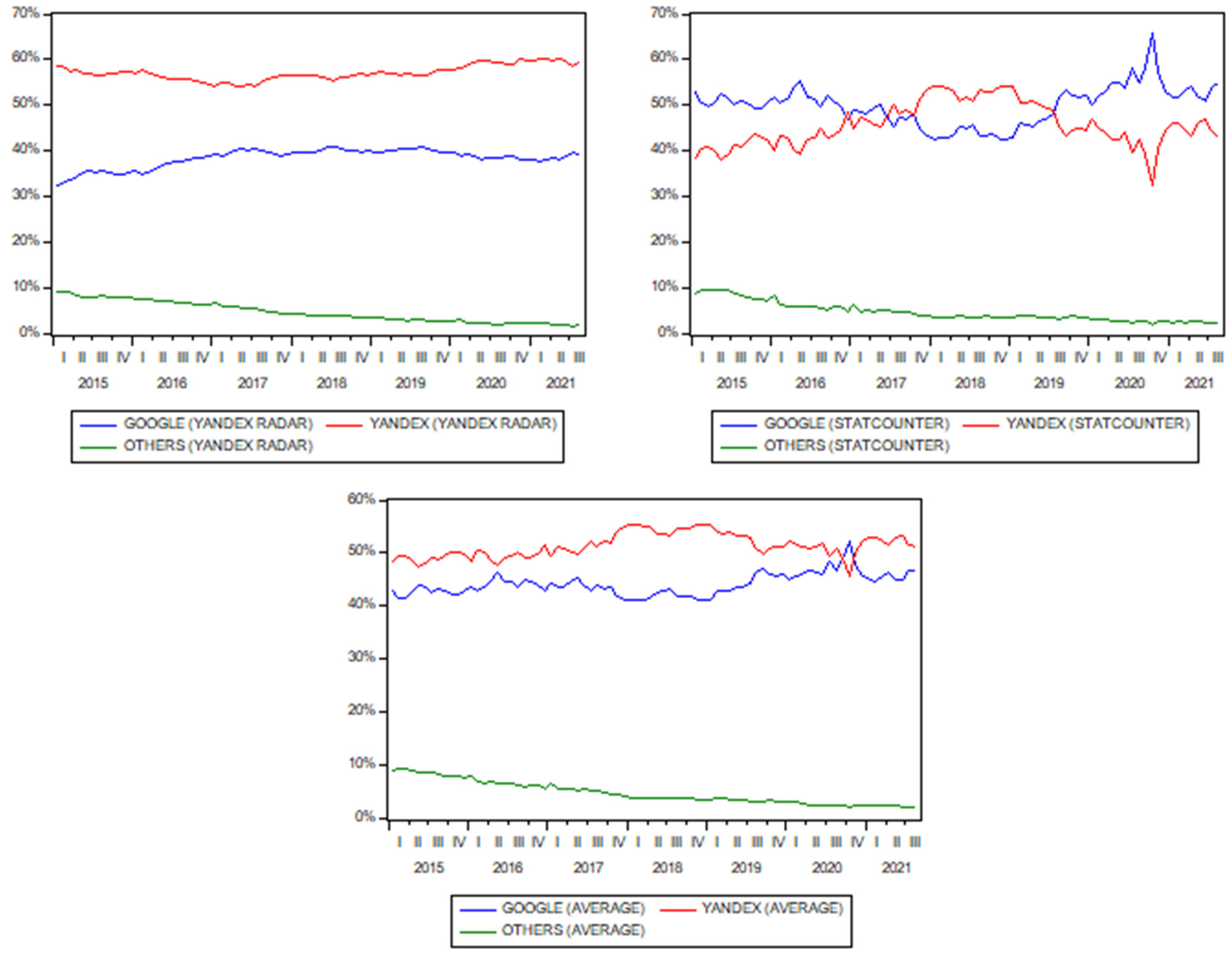
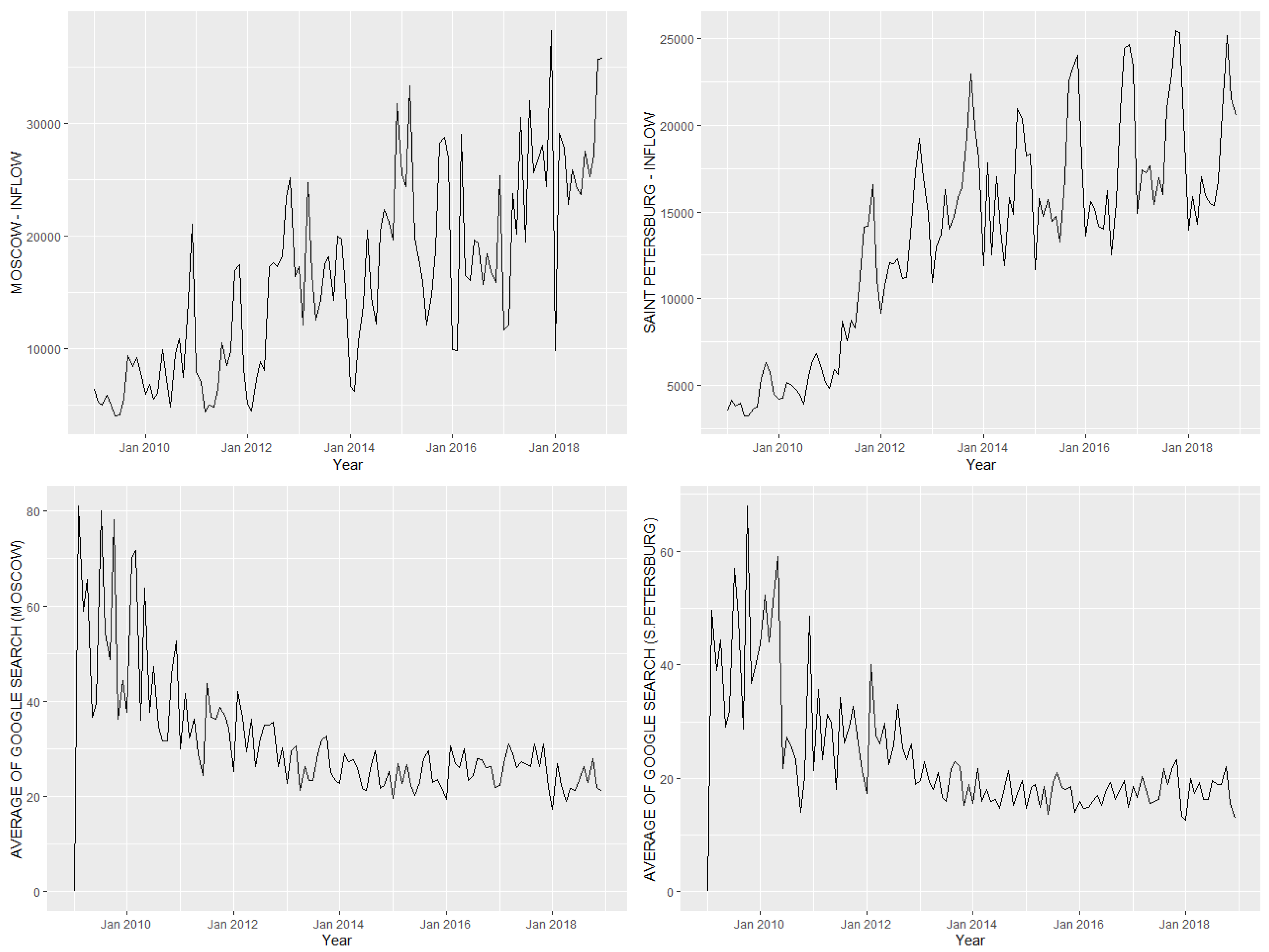
3.2.2. Search Volume Data
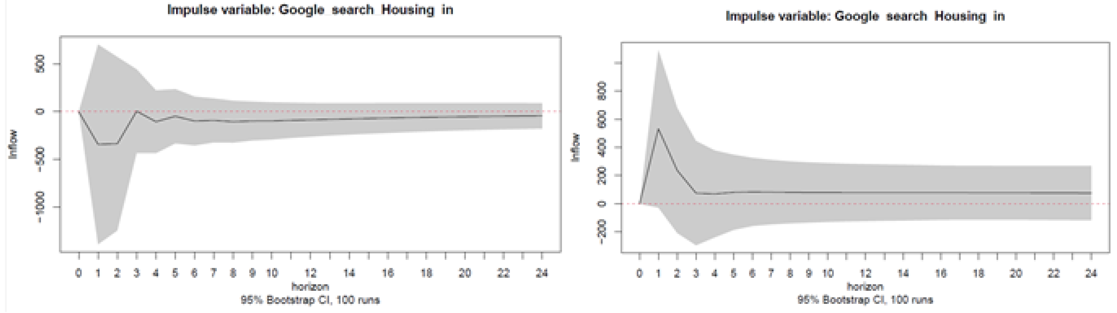
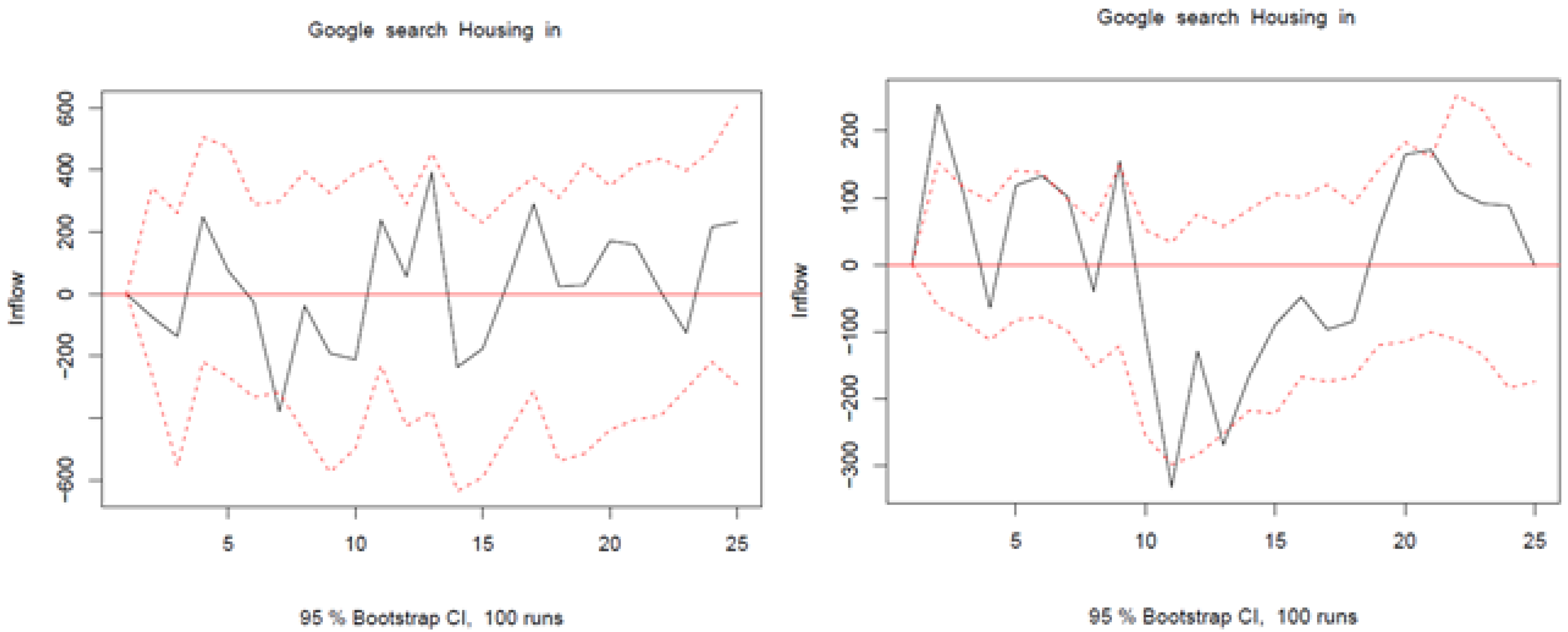
Russia has two search engines that take up most of the market: Yandex, and Google. In this regard, we remark that the computation of market shares for search engines is not straightforward—it can be controversial (https://www.conductor.com/blog/2014/05/shouldnt-trust-comscores-numbers-search-engine-market-share-data, accessed on 1 October 2021), and different analytical services may provide different numbers. In the case of Russia, the two most well-known analytical services are Yandex Radar (https://radar.yandex.ru/search?period=all&group=month, accessed on 1 October 2021) and StatCounter (https://gs.statcounter.com/search-engine-market-share/all/russian-federation, accessed on 1 October 2021). We report in Figure 1 the market shares of the Yandex and Google search engines since the beginning of 2015 for all platforms provided by these two services, together with their average (2015 was the first year when both analytical services were available).
StatCounter shows that Google was the top search engine in Russia for most of the studied period, while the opposite is true for Yandex Radar. Given that investigating which online analytical service is more reliable goes beyond the scope of this work, we focused our attention on their simple average, and we observed that Google had a market share in the 40–45% range, compared with a market share of 50–55% for Yandex. As we anticipated in the Introduction, Yandex provides only a limited amount of free monthly data, so we had to use Google search data for our work. Even though the latter does not appear to be the main search engine in Russia, its high market share guarantees that its data can still provide useful insights for this research.
Google Trends is a website by Google that publishes a standardized index known as the Google Index (GI), which estimates the popularity of a particular search query relative to the total number of searches in the same period in a specific region, and whose scale ranges from 0 to 100.
Although the general reach of Google Trends in Russia is wide, we found that the availability of online searches for our research purposes was quite limited, and search volumes were mostly available only from 2009 onwards. Therefore, we decided to focus only on the regions with the largest migration inflows, given that the online searches for the intentions to migrate were available only for these regions.
The top 10 regions by total immigration flow in 2018 (see Table 2) represented the starting point that we used to look for online search queries.
After comparing the volumes of migration flows in Russian regions with the availability of online search queries, we decided to choose Moscow and Saint Petersburg, which account for 12% of the total migration inflow. Even though the number of migrants in these cities is comparable to the migration inflows into other regions, the number of online searches for the other regions is almost insignificant compared to these two cities.
The choice of keywords for migration research is not predefined and clear-cut, unlike studies dealing with unemployment (for example), where the set of keywords “work” (“рабoта”) and “vacancies” (“вакансии”) is generally enough to obtain a good estimate of the intentions to find a job; see [5] and references therein for more details. It is for this reason that Böhme et al. [2] used a wide range of words that could potentially reflect an intention to move, including indirect interest in economic and legal issues—using, for example, keywords such as “GDP” and “passport”. According to the previously cited Russian studies dealing with migration, the main factors that explain the decision to emigrate are finding a job in the region of interest and finding an apartment. Therefore, we used not only the general query indicating the interest in emigrating (“переезд в «название региoна»”), but also queries on job and housing searches (“рабoта в «название региoна»”, “жилье в «название региoна»”). This choice allows us to focus on capturing the intentions to move from one region to another, whereas other queries may not indicate the direct intention to relocate. Moreover, we avoided the queries including the word “migration” (“миграция”) and its derivatives because they may be associated only with a general interest in migration policy. Furthermore, we specified the name of the region to exactly identify the direction of migration. We chose these three queries because they are the most popular search queries in each respective group of words concerning relocation, finding a job, and finding a place to live. As a result, compared to [2], our choice of keywords may provide an underestimated number of intentions to emigrate, but the willingness to move in our case is much more certain, and contains a specific geographical component.
We used the previous three queries separately for the in-sample analysis to examine the effect of each query on the migration flow. For forecasting purposes, we also considered the average of these three time series to reduce the number of variables involved, and to improve the forecasting efficiency; see e.g., [4,69] for details.

4. Results

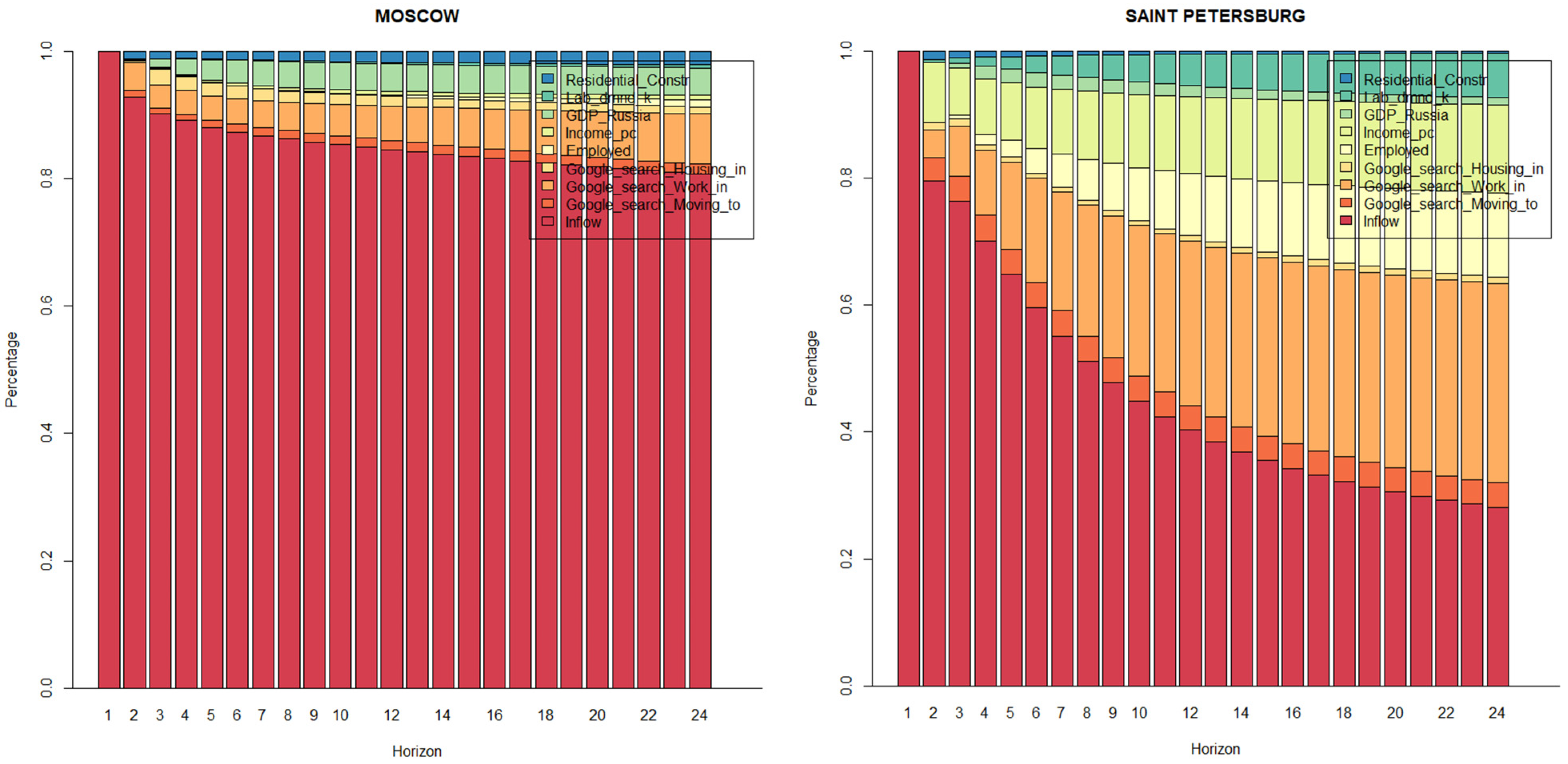
4.1. In-Sample Analysis

The monthly migration inflows in Moscow and Saint Petersburg, and the monthly averages for the three Google searches (“переезд в «название региoна»”,“рабoта в «название региoна»”,“жилье в «название региoна»”), are reported in Figure 2.
A first look at the data seems to show a certain degree of seasonality in the monthly inflows, particularly for Saint Petersburg. Therefore, we formally tested for seasonality using a battery of tests for the data in levels and in log-levels, which are reported in Table 3. More specifically, we used the F-test for seasonality based on the joint significance of seasonal dummies in a non-seasonal ARIMA model (where the latter is selected using the Hyndman-Khandakar algorithm [70]), the Friedman [71] test, the Kruskal–Wallis test [72], the QS test by Maravall [73]—which is a variant of the Ljung–Box test computed on seasonal lags—and the Welch test [74]. We also implemented the Ollech–Webel [75] test, which is a machine learning (ML) classification approach that first performs a recursive feature elimination algorithm using random forests to identify the most informative seasonality tests, and then uses their p-values as predictors within a single conditional inference tree to determine whether a time series has a significant seasonal component or not.
The seasonality tests highlighted a significant seasonal component, so we employed seasonal ARIMA models and VAR/VEC models allowing for seasonality when modeling the monthly inflow data.

4.1.1. Univariate Models

The best seasonal and non-seasonal ARIMA models, with and without Google search data, found using the Hyndman and Khandakar [70] algorithm with the corrected Akaike criterion (AICC) proposed by [76,77], are reported in Table 4 for both Moscow and Saint Petersburg. For the sake of interest, Table 4 also reports the Bayesian information criterion (BIC) for each selected model.
Seasonal models have lower information criteria than non-seasonal models, and this is particularly true for Saint Petersburg, while the differences are much smaller for Moscow inflow data, thus confirming the previous seasonality tests. The Moscow data have a non-seasonal unit root, while the inflow data for Saint Petersburg display both a seasonal and non-seasonal unit root. Interestingly, (S)ARIMA models augmented with Google search data as exogenous regressors almost always show worse information criteria than the baseline models without Google data (The coefficients of the Google search data were never statistically significant across all models considered. These results are not reported for reasons of space, but are available from the authors upon request). No qualitative differences are found when using data in levels and data in log-levels (We remark that the information criteria for the data in levels and in log-levels cannot be directly compared because the datasets used are different).

4.1.2. Multivariate Models

Consistent with previous literature dealing with Russian migration research, we employed multivariate models for a set of variables including the migration inflows, the estimated Russian monthly GDP, the nominal wage of employees (per capita), the residential construction volume (in thousand square meters), the number of employed people in the 15–72 age group, the employers’ need for employees (according to the Russian Federal Service for Labor and Employment), and the Google search data for the queries about moving in a certain region, about finding work, and about finding housing.
The information criteria selected a VAR (1) model for both Moscow and Saint Petersburg. Given the presence of seasonality, we estimated all multivariate models with centered seasonal dummies, which sum to zero over time and, therefore, do not affect the asymptotic distributions of testing procedures; see Johansen [78,79] for more details. For ease of interpretation and the sake of interest, we report the orthogonalized impulse responses (The orthogonalized impulse responses are derived from a Choleski decomposition of the error variance–covariance matrix Σ = PP′, with P being lower triangular; see Lütkepohl [80] for more details) from a shock in Google searches on migration inflows in Moscow and Saint Petersburg in Figure 3 and Figure 4, respectively; the forecast error variance decompositions (The forecast error variance decomposition is based upon the orthogonalized impulse response coefficient matrices, and shows the contribution of the variable j to the h-step forecast error variance of variable k; see Lütkepohl [80] for more details) for the migration inflows are reported in Figure 5, while the full results are available from the authors upon request.
Figure 3 and Figure 4 show that the effects of shocks in internet searches on migration inflows are not significant for queries related to emigration and housing searches, while there are significant negative effects for queries related to job searches. In the latter case, it appears that a one-time shock in internet search queries results in a negative migration inflow after approximately five months. The forecast error variance decompositions in Figure 5 show that the variances in migration inflows are mostly affected by their own variances, but the effects of online job searches and the numbers of employed people become stronger in later periods—particularly for Saint Petersburg.
The negative relationship between online job searches and migration inflows is probably due to immigrants moving to the regions bordering Moscow and Saint Petersburg, because of the high cost of living and traffic congestion in these two metropolises; see e.g., [37,81,82,83,84].
Given the evidence of non-stationarity that emerged from the previous univariate analysis, for the sake of generality and interest, we also considered a VEC model following the standard sequential specification procedure based on pretests for unit roots and co-integration. We tested for co-integration using the Johansen trace test with centered seasonal dummies, and we rejected the null hypothesis of no co-integration for both Moscow and Saint Petersburg. We estimated a VEC (1) model with six co-integration relationships and a constant term in the co-integration equations for both cities. The orthogonalized impulse responses from a shock in Google searches on migration inflows in Moscow and Saint Petersburg are reported in Figure A3 and Figure A4, respectively, in Appendix B, while the forecast error variance decompositions for the migration inflows are reported in Figure A5, and the full results are available from the authors upon request. The IRFs and the FEVDs obtained with the VEC models are qualitatively similar to those estimated with VAR models in levels, confirming a significant negative effect of online job searches on migration inflows (for Saint Petersburg), and a much larger importance of Google searches for Saint Petersburg than for Moscow.

4.2. Out-of-Sample Forecasting Analysis

The last step to evaluate the ability of Google search data to predict internal migration in Russia was to perform an out-of-sample forecasting analysis for both Moscow and Saint Petersburg, in order to forecast the monthly inflows using several competing models, with and without Google data, over different time horizons. The data from January 2009–September 2015 were used as the first training sample for the models’ estimation, while the data from October 2015–December 2018 were left for out-of-sample forecasting using an expanding estimation window.

4.2.1. Short-Term Forecasts: One-Step-Ahead Forecasts

Three classes of models were considered for short-term forecasts, for a total of 20 models:
(1)
ARIMA models with the dependent variable represented by the monthly inflows in levels or log-levels (2 models);
(2)
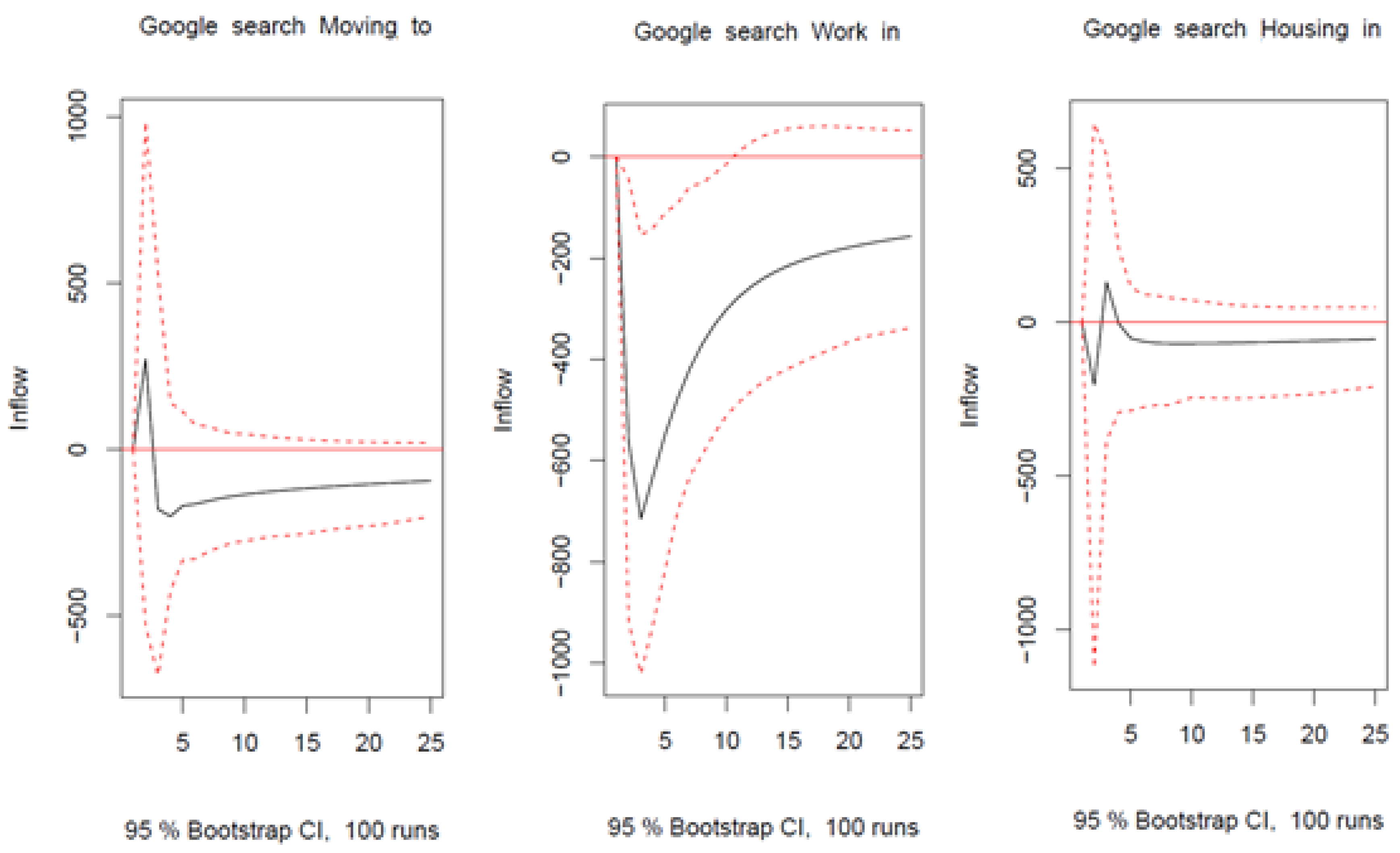
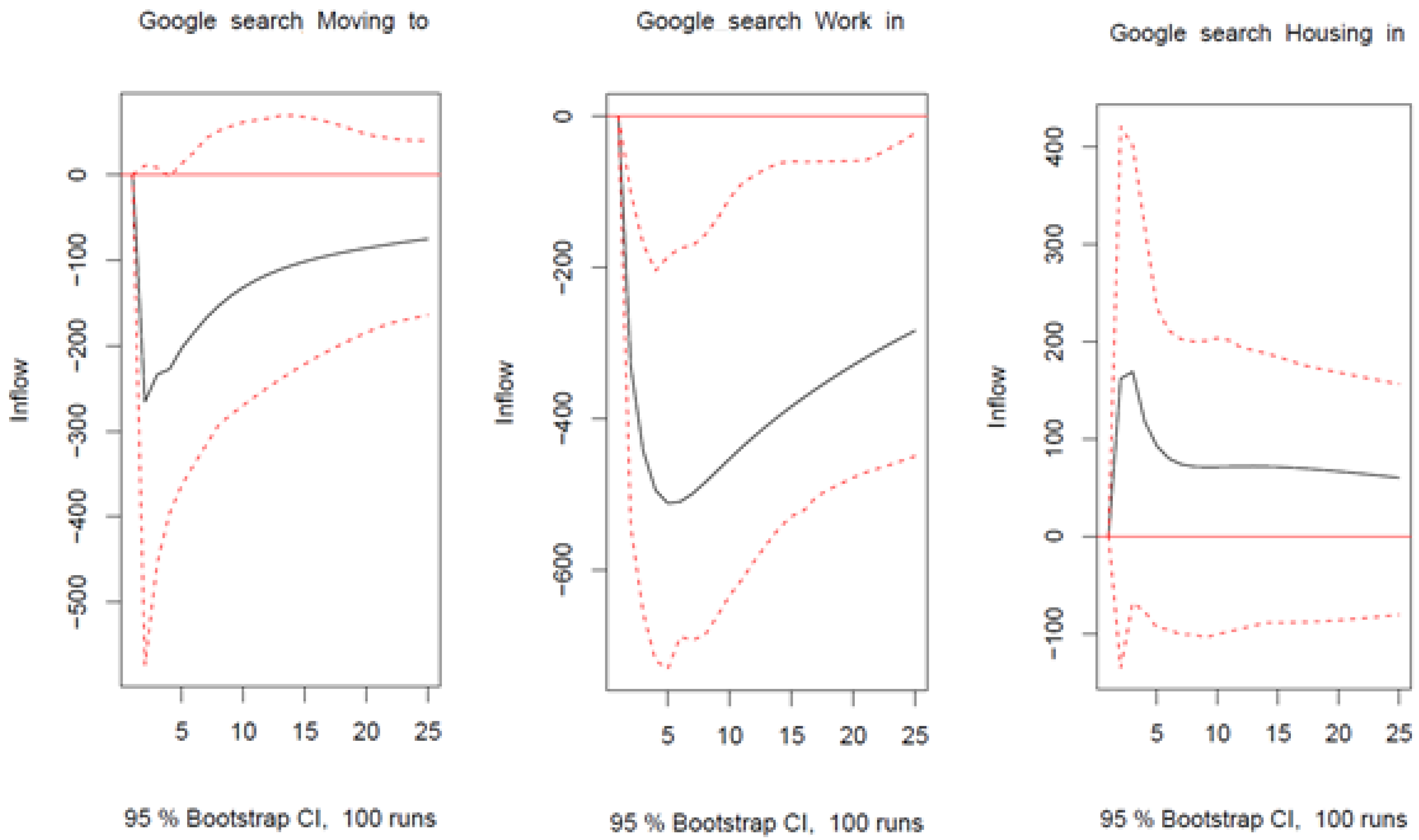
Google-augmented ARIMA-X models with the variables in levels or log-levels (8 models): we considered lagged Google search data for the queries about moving in a certain region and queries about jobs and housing, as well as the average of these three queries;
(3)
Seasonal ARIMA (SARIMA) models with and without Google search data, with the variables in levels or log-levels (10 models).
(4)
Additional models could surely be added, but this selection already gives important indications whether Google search data are useful for forecasting the monthly migration inflows in Moscow and Saint Petersburg. A summary of the models’ performances according to the mean squared error (MSE), the mean absolute error (MAE), and the mean absolute percentage error (MAPE) is reported in Table 5 (The optimal seasonal and non-seasonal ARIMA models, with and without Google search data, were estimated using the Hyndman and Khandakar [70] algorithm at each iteration of the forecasting procedure).
In general, Google-augmented time-series models forecasted the monthly inflows better than models without Google data. However, the simple SARIMA model with data in logs turned out to be the best model for Saint Petersburg (even though Google-based models were close); this result was expected due to the strong local seasonality in monthly inflows—in contrast to Moscow, where the seasonality was barely significant. This phenomenon may also explain why models with the variables in logs forecasted better than models with the variables in levels for Saint Petersburg, whereas the opposite was true for Moscow. Among Google search terms, queries about moving in a certain region or the averages of all three queries provided better forecasts than the other choices.

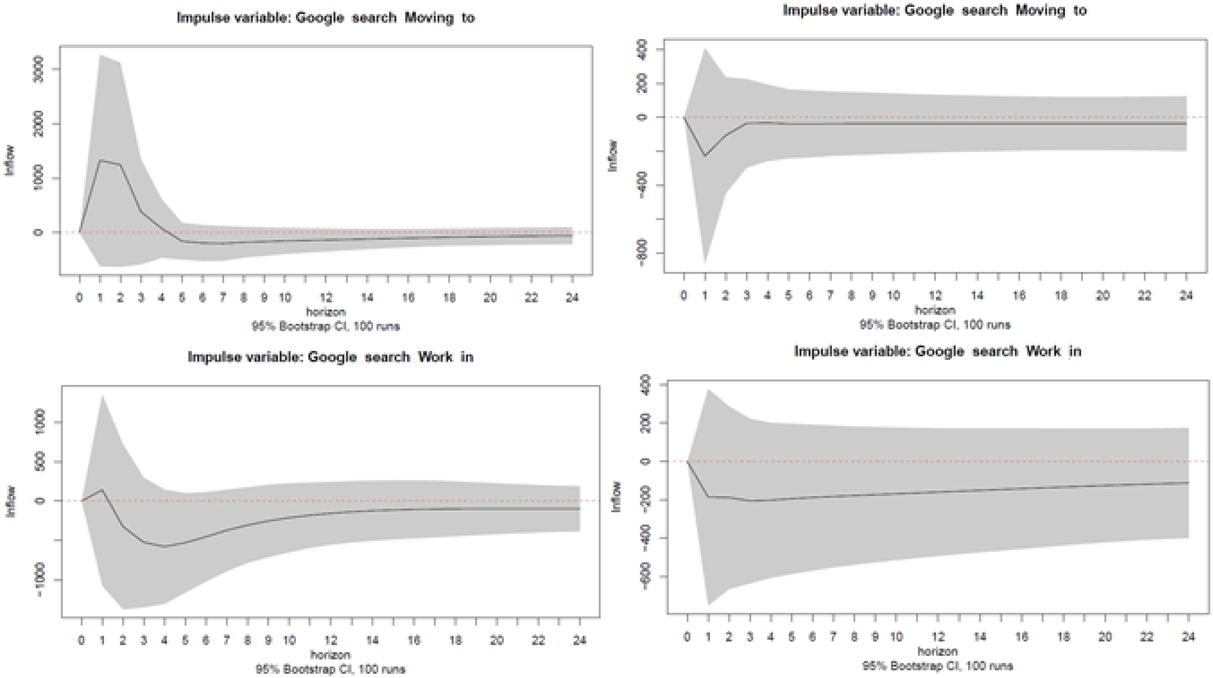
4.2.2. Long-Term Forecasts: 24-Step-Ahead Forecasts

The previous univariate models can also be used for long-term forecasting, but it is well known that their forecasting ability quickly degrades; see Hyndman and Athanasopoulos [85] and references therein for more details. Moreover, if exogenous variables are present, multivariate models have to be used to build long-term forecasts.
More specifically, we used three classes of models to build long-term 24-step-ahead forecasts:
(1)
VAR models with centered seasonal dummies, with and without Google data, with the variables in levels, log-levels, first differences, or log-returns (12 models);
(2)
VEC models with centered seasonal dummies, with and without Google data, with the variables in levels or log-levels (6 models);
(3)
Seasonal ARIMA models, as simple univariate benchmark models, with the variables in levels or log-levels (2 models).
As for the Google search queries, we considered three possible variants: no Google data, the average of the three Google search queries, or all three Google search queries together. A summary of the models’ performances according to the mean squared error (MSE), the mean absolute error (MAE), and the mean absolute percentage error (MAPE) is reported in Table 6.
In general, multivariate models with Google data forecasted better than multivariate models without Google data, and much better than simple SARIMA models (as expected). In the case of Moscow, the VAR model with the variables in log levels and the average of the Google search queries was the best, while VAR models with the variables expressed in log returns (with and without Google data) provided the best forecasts; therefore, this forecasting evidence confirmed the initial in-sample analysis, where the evidence of non-stationarity was much stronger for Saint Petersburg than for Moscow. Interestingly, the VEC models performed poorly—in some cases even worse than SARIMA models; these results were not a surprise, because the large variance in the estimators for co-integrated models in small–medium samples is a well-known issue in the econometric literature; see [86,87,88] for more details. Moreover, Fantazzini and Toktamysova [89] showed that the sampling noise of Google data can exacerbate this inference problem, and using the averages of Google data can solve this issue to some extent (but not completely); this is also what we found with our data, where models with the averages of Google data often performed better than models with the separate Google search queries.
These results are consistent with a large body of the forecasting literature, which shows that Google-based models outperform their competitors; see, for example, [4,5,9,90] and references therein.

5. Discussion and Conclusions

There is an increasing body of literature that shows that Google-based models significantly outperform most of their competitors in several economic and financial applications; see [1] for a review. Böhme et al. [2] analyzed the potential of online search data for predicting migration flows for the first time, and they showed that this approach improved the forecasting performances of conventional models of migration flow; moreover, it provided real-time forecasts ahead of official statistics.
Following this literature, this paper used monthly migration data, Google search volume data, and macroeconomic variables for the 2009–2018 time period to analyze how these variables affected migration inflows for the two Russian cities with the largest migration inflows: Moscow and Saint Petersburg. The choice of keywords for migration research was not predefined and clear-cut, unlike previous studies dealing with unemployment or financial and economic forecasting. We followed previous Russian studies that showed that the main factors explaining the decision to emigrate are finding a job (in the region of interest) and finding an apartment. Therefore, we used not only the general query indicating the interest in emigrating (“переезд в «название региoна»”), but also queries on job and housing searches (“рабoта в «название региoна»”, “жилье в «название региoна»”). We chose these three queries because they are the most popular search queries in each respective group of words concerning relocation, finding a job, and a place to live. As a result, compared to [2], our choice of keywords may provide an underestimated number of intentions to emigrate, but the willingness to move is more certain, and it contains a specific geographical component.
The empirical analysis did not provide evidence that the more people search online, the more they relocate to other regions, but we found that a one-time shock in internet search queries results in a negative migration inflow after approximately five months. We then performed an out-of-sample forecasting analysis to forecast the monthly inflows using several competing models, with and without Google data, over different time horizons ranging from 1 month to 24 months ahead. In terms of short-term forecasting, Google-augmented time-series models usually forecasted the monthly inflows better than models without Google data. However, the simple SARIMA model with data in logs turned out to be the best model for Saint Petersburg, thanks to the strong local seasonality in monthly inflows, whereas this was not the case for Moscow, where the monthly seasonality was barely significant.
In terms of long-term forecasting, multivariate models with Google data forecasted better than multivariate models without Google data, and much better than univariate models. Interestingly, the VEC models performed poorly—in some cases even worse than simple univariate models—thus confirming well-known estimation problems in small–medium samples, which can be further exacerbated by the sampling noise of Google data. These results also held after a set of robustness checks that considered multivariate models able to deal with potential parameter instability and with a large number of regressors—potentially larger than the number of observations.
Our empirical evidence showed that Google Trends does help to forecast migration inflows in the two Russian cities with the largest migration inflows (Moscow and Saint Petersburg). As recently highlighted by Nikolopoulos et al. [9,10], the lack of reliable hard data limits the possibility of policymakers making informed decisions, and this is why they suggested employing auxiliary data from social media, such as Google Trends. Given that migration inflows represent a sensitive social issue in Russia, the option to improve the modeling and forecasting of these flows by using auxiliary data such as Google Trends can be of great help to local policymakers. This improvement is even more important if we consider that a part of these migration inflows is represented by illegal immigrants, who are not included in official statistics, but can be revealed by Google Trends.
The availability to policymakers of a wide array of leading indicators for migration dynamics—ranging from online search data to telecommunications data—can be useful to plan and implement more realistic migration policies that can significantly help the inclusion process of migrants; see [11] for a larger discussion.
The negative relationship between online job searches and migration inflows is probably due to immigrants moving to the regions bordering Moscow and Saint Petersburg, because of the high cost of living and traffic congestion in these two metropolises; see e.g., [37,79,82]. An empirical analysis also including these bordering regions would require spatial econometric models able to deal with situations where the number of variables is larger than the number of timepoints for the data; see e.g., [91,92] and references therein. Given that this issue goes beyond the scope of this paper, and the size of the paper is already quite substantial (The authors want to thank an anonymous reviewer for highlighting the initial excessive length of the paper), we leave this issue as an avenue for further research.
Another possibility of future work will be to check how the empirical evidence found in this work would change when using Yandex search data in place of Google search data. To reach this aim, a direct agreement between Russian policymakers and Yandex would probably be necessary to enable access to long time series of monthly search data, which are currently unavailable. The inclusion of such data would likely considerably improve the forecasting performances of the models proposed in this work, so we leave it as a compelling topic for further work.

Author Contributions

Conceptualization, D.F. and J.P.; methodology, D.F., J.P., A.M. and A.K.; software, D.F., J.P. and A.M.; validation, D.F., A.M., and A.K.; formal analysis, D.F., J.P. and A.M.; investigation, D.F, J.P., A.M. and A.K.; data curation, D.F. and J.P.; writing—original draft preparation, D.F. and J.P.; writing—review and editing, D.F., J.P. and A.K.; visualization, D.F. and J.P.; supervision, D.F. and A.K.; project administration, D.F. and A.K.; funding acquisition, D.F., A.M. and A.K. All authors have read and agreed to the published version of the manuscript.

Funding

Dean Fantazzini, Alexey Mironenkov and Alexey Kurbatskii gratefully acknowledge financial support from the grant of the Russian Science Foundation n. 20-68-47030.

Institutional Review Board Statement

Not applicable.

Informed Consent Statement

Not applicable.

Conflicts of Interest

The authors declare no conflict of interest.

Appendix A

Google Trends is a website (https://trends.google.com, accessed on 1 October 2021) that reports the standardized volume of Google searches for a keyword or a topic. Google Trends calculates the ratio of the number of online searches for a specific keyword (or topic) K in a given geographical region a, on a particular day t (Ka,t), to the total amount of searches for the same day and region (Ta,t): Ra,t = Ka,t/Ta,t. The obtained time series is then divided by the value of the day in which it reaches the maximum level, and multiplied by 100. The Google index (GI) for a specific keyword K on day t, and in the area a, is thus given by GIKa,t = [100 Ra,t/maxt (Ra,t)]. Google Trends only tracks queries with a minimum volume, due to privacy considerations; if the search volume is too low, a value of zero is reported (In the case of zero values, the GIs were linearly rescaled using a small positive constant, following the approach proposed by Fantazzini and Toktamysova [89]). The data are available from an intraday time frequency up to a monthly frequency (which was our case), depending on the selected time range. The longer the selected time sample, the lower the frequency provided by Google Trends (the lowest frequency possible is monthly data). Note that Google Trends allows comparison of the search volumes of up to five search terms, or up to a maximum of 30 search terms grouped in a single entry using quotation marks (to return searches that match an exact expression), and using the + or − signs between the search terms to include or exclude search terms, respectively. The data are available since 2004; see https://support.google.com/trends for more details (accessed on 1 October 2021).
An example of the Google Trends interface to download the monthly data for the keywords “Рабoта в Мoскве” (=”Job in Moscow”) searched in Russia from 1 January 2009 until 31 December 2018 is reported in Figure A1.
Figure A1. Google Trends data for the keywords “Рабoта в Мoскве”, searched in Russia. Sample: 01/01/2009–31/12/2018.
Forecasting 03 00048 g0a1
The monthly GIs can be downloaded as a csv file by clicking on the arrow on the right, as highlighted in Figure A1. Given that the manual download of the GIs for several keywords can become too burdensome, it can be executed using an R script and the gtrendsR package, as reported below (see also in Figure A2):
library(gtrendsR)
dat=gtrends(“Рабoта в Мoскве”, geo = “RU”, time = “2009-01-01 2018-12-31”)
plot(dat)
Figure A2. Google Trends data for the keywords “Рабoта в Мoскве”, searched in Russia. Sample: 1 January 2009–31 December 2018. Data downloaded using the gtrendsR package.
Forecasting 03 00048 g0a2
We remark that Google Trends data are computed using a sampling method, so the results may be slightly different if the data are downloaded on different days. A possible way to decrease the sample variability is to compute the GIs as the simple average of different data downloads performed over different days. We also tried this approach as a robustness check, but we decided to use the original raw data coming from the single downloads because we found that using the raw data does not alter the final results, similarly to the findings of Fantazzini and Toktamysova [89] and D’Amuri and Marcucci [5].
Google Trends has both advantages and limitations when forecasting migration. In general, Google Trends has several advantages in terms of economy, coverage, and immediacy: it is free of charge, and can cover larger sets of population than some of the traditional data sources, which may suffer from sample size limits. Moreover, it can allow researchers to monitor immigrants’ intentions almost in real time. In this regard, the main advantage of online search queries is the possibility of anticipating immigrants’ movement, as highlighted by Böhme et al. [2], who validated this proposition by comparing the Gallup World Poll data about emigration (This was a survey conducted over more than 160 countries, with the aim of finding whether the local individuals were planning to move to another country and, if so, whether the plan would take place within 12 months; see http://gallup.com, accessed on 1 October 2021, for more details) with the results obtained with Google Trends, and found that Google Trends data can indeed nowcast the “genuine migration intention”.
However, Google Trends data also have their limitations: for example, it is well known that online users may not represent the whole population, and these data may require significant cleaning; see Jun et al. [1], Nikolopoulos et al. [10], and references therein. The impossibility of tracking specific categories of users may determine migration policies that perpetuate discrimination or neglect the needs of some groups. For these reasons, the latest research efforts try to combine online big data with more traditional data sources; see Salini et al. [93] and Iacus and Porro [94] for more details.
Despite these limitations, an increasing body of literature shows that Google Trends and other online big data can still improve the understandings of migration patterns; see Hawelka et al. [29], Zagheni et al. [30], Moise et al. [31], Iacus and Porro [94], and Sîrbu et al. [11] for more details.

Appendix B

Figure A3. VECM (1) with centered seasonal dummies: orthogonalized impulse responses from a shock in Google searches on migration inflow in Moscow over 24 months.
Forecasting 03 00048 g0a3
Figure A4. VECM (1) with centered seasonal dummies: orthogonalized impulse responses from a scheme 24 months.
Forecasting 03 00048 g0a4
Figure A5. Forecast error variance decomposition of the VECM (1) with centered seasonal dummies: Moscow (left panel); Saint Petersburg (right panel).
Forecasting 03 00048 g0a5

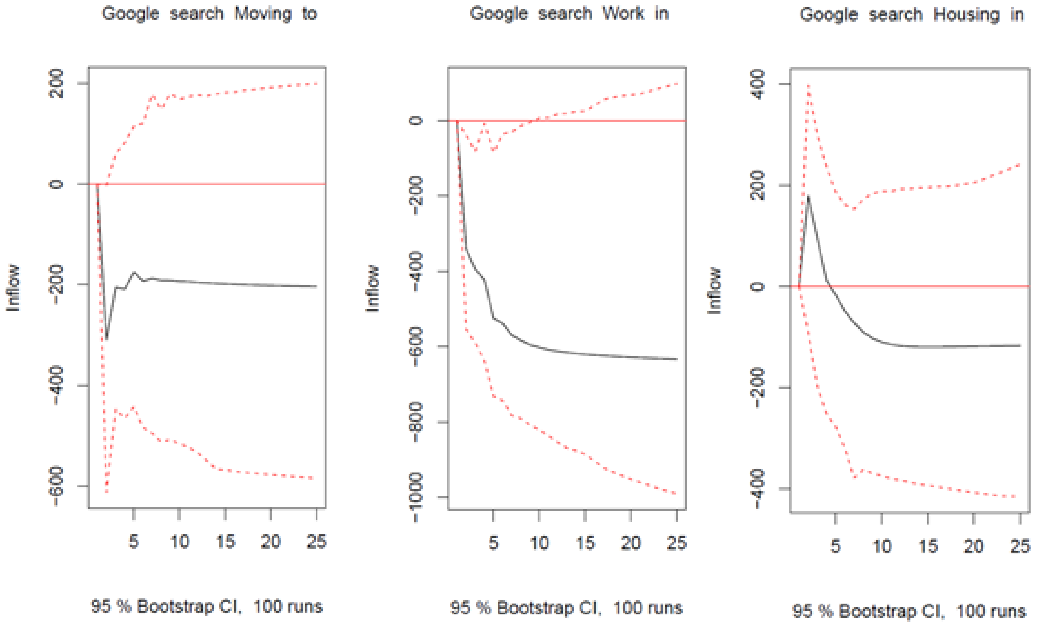
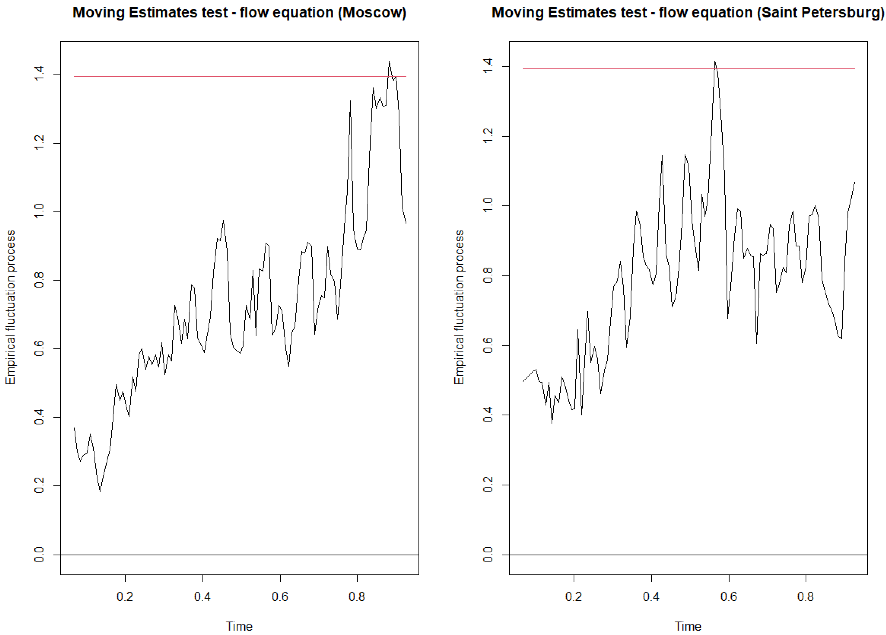
Appendix C. Robustness Checks

We wanted to check how our previous results changed with models able to deal with potential parameter instability and with a large number of regressors—potentially larger than the number of observations. To achieve this goal, we employed the time-varying VAR model proposed by Casas and Fernandez-Casal [95] and Casas et al. [96], and a set of multivariate shrinkage estimation methods.

Appendix C.1. Parameter Instability

We tested for the structural stability of our VAR (1) models using the generalized fluctuation tests discussed in [97,98,99]. For the sake of interest and space, we report below only the fluctuation test based on the moving OLS estimates for the VAR equation of the monthly migration flow in Moscow and Saint Petersburg, while the full results are available from the authors upon request (This (large) class of fluctuation tests for testing, monitoring, and dating structural changes in linear regression models is implemented in the R package strucchange).
Figure A6 and the battery of tests that we computed to test for structural stability highlighted that the evidence for parameter instability is mild or non-significant. Nevertheless, we decided to implement the time-varying coefficient vector autoregressive model (TVVAR) proposed by Casas and Fernandez-Casal [96] and Casas et al. [100] to take any potential parameter instability into account:
Y t = Φ 0 , t + i = 1 p Φ i , t Y t i + u t , u t W N ( 0 , Σ t )
where the elements of Φi,t are unknown functions of either the rescaled time value τ = t / T with τ ∈ (0, 1), or of a random variable at time t. The variance–covariance matrix t can also be time-varying. If the matrices Φi,t are a function of τ, then the TVVAR model is locally stationary in the sense of Dahlhaus [101], which means that the functions in the matrices are constant or change smoothly over time. In this case, the TVVAR model (2) has a well-defined Wold representation given by:
Y ¯ t = j = 0 Ψ j , t u t j
with | Y ¯ t Y t | → 0 almost surely, Ψ 0 , t = I n , Ψ s , t = j = 1 s Ψ s j , t Φ j , t for horizons s = 1, 2,…, and where Ψ s , t represent the time-varying coefficient matrices of the impulse response function (TVIRF); see [95] for more details. The orthogonal TVIRF can be computed using Ψ j , t P t instead of Ψ j , t , where P t is the lower triangular matrix obtained by employing the Cholesky decomposition of Σ t at time t, given by Σ t = P t P t .
The TVVAR model (2) can be estimated using a multivariate nonparametric Nadaraya–Watson estimator that minimizes a smoothed weighted sum of squared residuals; see [96] for a detailed analysis of the asymptotic properties of this kernel estimator (The TVVAR model is implemented in the R package tvReg).
The orthogonal impulse responses from a shock in Google online searches on migration inflow in Moscow (left column) and Saint Petersburg (right column) are reported in Figure A7, where the values reported are the means of the time-varying IRF over each time period.
Figure A6. Fluctuation test based on the moving OLS estimates for the VAR equation of the monthly migration flow in Moscow and Saint Petersburg, with the boundary for the 5% confidence level (red line). The standardized sample cover the period 2009–2020.
Forecasting 03 00048 g0a6
Figure A7. Orthogonal impulse responses from a shock in Google online searches on migration inflow in Moscow (left column) and Saint Petersburg (right column) using a TVVAR (1) model. The values reported are the means of the time-varying IRF over each period.
Forecasting 03 00048 g0a7aForecasting 03 00048 g0a7b
Similar to the baseline case, a one-time shock in online Google searches related to emigration and job queries has a negative effect on migration inflows but, in contrast to the baseline case, these effects are no more significant.
The lack of significance of the IRFs can probably be explained by the larger variances in the TVVAR model estimates compared to traditional VAR models with constant parameters, and by the weak evidence of model instability, which makes the TVVAR model more inefficient.

Appendix C.2. Additional Lags

The simple VAR (1) model used in the baseline case can be an efficient way to deal with several variables, but it is hardly realistic, considering that the decision and the entire process to emigrate may take several months, at the very least (The first author of this paper immigrated to Moscow in August 2007; if the initial planning phase is considered, together with the time needed to satisfy all the administrative and migration requirements necessary for the physical transfer, the entire process took up to 1 year). Unfortunately, given the limited size of our dataset, VAR models with more than six lags were numerically unstable or simply impossible to estimate. Therefore, we resorted to multivariate shrinkage estimation methods that can be applied to high-dimensional VAR models with dimensionality potentially larger than the number of observations.
More specifically, we considered the multivariate ridge regression by Hoerl and Kennard [100]. If we rewrite the VAR model described in Equation (1) in a more compact form, as follows:
Y = XB + U
where Y is a (Tp) × n matrix collecting the temporal observations of all endogenous variables, X is a (Tp) × (np+1) matrix collecting the lags of the endogenous variables and the constants, B is a (np + 1) × n matrix of coefficients, and U is a (Tp) × n matrix of error terms, then the multivariate ridge regression estimator of B can be obtained by minimizing the following penalized sum of squared errors:
B ^ R i d g e ( λ ) = arg min B 1 T p Y X B F 2 + λ B F 2
where A F = i j a i j 2 is the Frobenius norm of a matrix A, and λ ≥ 0 is known as the regularization parameter or the shrinkage parameter. The ridge regression estimator B ^ R i d g e ( λ ) has a closed form solution given by:
B ^ R i d g e ( λ ) = ( X X + ( T p ) λ I ) 1 X Y , λ 0
The shrinkage parameter λ can be automatically determined by minimizing the generalized cross-validation (GCV) score by Golub, Heath, and Wahba [102]:
G C V ( λ ) = 1 T p I H ( λ ) Y F 2 / [ 1 T p T r a c e ( I H ( λ ) ) ] 2
where H ( λ ) = X ( X X + ( T p ) λ I ) 1 X .
Given our previous discussion, we considered a VAR (12) model estimated with the ridge regression estimator. The orthogonal impulse responses from a shock in Google online searches on migration inflow in Moscow (left column) and Saint Petersburg (right column) are reported in Figure A8.
Figure A8. Orthogonal impulse responses from a shock in Google online searches on migration inflow in Moscow (left column) and Saint Petersburg (right column), using a VAR (12) model estimated with the ridge regression estimator.
Forecasting 03 00048 g0a8aForecasting 03 00048 g0a8b
The estimated IRFs are similar to the baseline case, except for one-time shocks in online searches related to emigration, which have a positive effect on migration inflows in Moscow, thus confirming similar evidence reported in [2]. However, none of these effects are any more statistically significant.
We remark that we also attempted alternative multivariate shrinkage estimation methods for VAR models, such as the nonparametric shrinkage estimation method proposed by Opgen-Rhein and Strimmer [103], the full Bayesian shrinkage methods proposed by Sun and Ni [104] and Ni and Sun [105], and the semi-parametric Bayesian shrinkage method proposed by Lee et al. [106]; the results with these methods were qualitatively similar, but their computational performance was much worse in several cases; as such, we do not report them here for the sake of space and interest (These additional results are available from the authors upon request.), (All of the multivariate shrinkage estimation methods discussed in the text are implemented in the R package VARshrink).

References

  1. Jun, S.-P.; Yoo, H.S.; Choi, S. Ten years of research change using Google Trends: From the perspective of big data utilizations and applications. Technol. Forecast. Soc. Chang. 2018, 130, 69–87. [Google Scholar] [CrossRef]
  2. Böhme, M.H.; Gröger, A.; Stöhr, T. Searching for a better life: Predicting international migration with online search keywords. J. Dev. Econ. 2019, 142, 102347. [Google Scholar] [CrossRef]
  3. Choi, H.; Varian, H. Predicting the Present with Google Trends. Econ. Rec. 2012, 88, 2–9. [Google Scholar] [CrossRef]
  4. Fantazzini, D.; Fomichev, N. Forecasting the real price of oil using online search data. Int. J. Comput. Econ. Econom. 2014, 4, 4–31. [Google Scholar] [CrossRef]
  5. D’Amuri, F.; Marcucci, J. The predictive power of Google searches in forecasting US unemployment. Int. J. Forecast. 2017, 33, 801–816. [Google Scholar] [CrossRef]
  6. Bulut, L. Google Trends and the forecasting performance of exchange rate models. Journal of Forecasting. 2018, 37, 303–315. [Google Scholar] [CrossRef]
  7. Yu, L.; Zhao, Y.; Tang, L.; Yang, Z. Online big data-driven oil consumption forecasting with Google trends. Int. J. Forecast. 2019, 35, 213–223. [Google Scholar] [CrossRef]
  8. Borup, D.; Schütte, E.C.M. In Search of a Job: Forecasting Employment Growth Using Google Trends. J. Bus. Econ. Stat. 2020, 1–15. [Google Scholar] [CrossRef]
  9. Nikolopoulos, K.; Tsinopoulos, C.; Vasilakis, C. Operational research in the time of COVID-19: The ‘science for better’or worse in the absence of hard data. J. Oper. Res. Soc. 2021, 290, 99–115. [Google Scholar] [CrossRef] [PubMed]
  10. Nikolopoulos, K.; Punia, S.; Schäfers, A.; Tsinopoulos, C.; Vasilakis, C. Forecasting and planning during a pandemic: COVID-19 growth rates, supply chain disruptions, and governmental decisions. Eur. J. Oper. Res. 2020, 290, 99–115. [Google Scholar] [CrossRef]
  11. Sîrbu, A.; Andrienko, G.; Andrienko, N.; Boldrini, C.; Conti, M.; Giannotti, F.; Sharma, R. Human migration: The big data perspective. Int. J. Data Sci. Anal. 2021, 11, 341–360. [Google Scholar] [CrossRef]
  12. Ravenstein, E.G. The laws of migration. J. Stat. Soc. Lond. 1885, 48, 167–235. [Google Scholar] [CrossRef]
  13. Wilson, A. Entropy in Urban and Regional Modelling (Routledge Revivals); Routledge: Oxford, UK, 2013. [Google Scholar] [CrossRef]
  14. Willekens, F. Entropy, multiproportional adjustment and the analysis of contingency tables. Syst. Urbani 1980, 2, 171–201. [Google Scholar]
  15. Alonso, W. Systemic and Log-Linear Models: From Here to There then to Now and This to That; Discussion Paper 86-10; Center for Population Studies, Harvard University: Cambridge, MA, USA, 1986. [Google Scholar]
  16. Bijak, J.; Disney, G.; Findlay, A.M.; Forster, J.J.; Smith, P.W.; Wiśniowski, A. Assessing time series models for forecasting international migration: Lessons from the United Kingdom. J. Forecast. 2019, 38, 470–487. [Google Scholar] [CrossRef] [Green Version]
  17. Mayda, A.M. International migration: A panel data analysis of the determinants of bilateral flows. J. Popul. Econ. 2009, 23, 1249–1274. [Google Scholar] [CrossRef]
  18. Constant, A.F.; Zimmermann, K.F. Circular and Repeat Migration: Counts of Exits and Years away from the Host Country. Popul. Res. Policy Rev. 2010, 30, 495–515. [Google Scholar] [CrossRef]
  19. Bijak, J. Forecasting International Migration in Europe: A Bayesian View. JSTOR 2011. [Google Scholar] [CrossRef] [Green Version]
  20. Ortega, F.; Peri, G. The effect of income and immigration policies on international migration. Migr. Stud. 2013, 1, 47–74. [Google Scholar] [CrossRef] [Green Version]
  21. Chort, I. Mexican migrants to the US: What do unrealized migration intentions tell us about gender inequalities? World Dev. 2014, 59, 535–552. [Google Scholar] [CrossRef]
  22. Docquier, F.; Peri, G.; Ruyssen, I. The Cross-country Determinants of Potential and Actual Migration. Int. Migr. Rev. 2014, 48, 37–99. [Google Scholar] [CrossRef] [Green Version]
  23. Dustmann, C.; Okatenko, A. Out-migration, wealth constraints, and the quality of local amenities. J. Dev. Econ. 2014, 110, 52–63. [Google Scholar] [CrossRef] [Green Version]
  24. Burkhauser, R.V.; Hahn, M.H.; Hall, M.; Watson, N. Australia Farewell: Predictors of Emigration in the 2000s. Popul. Res. Policy Rev. 2016, 35, 197–215. [Google Scholar] [CrossRef] [Green Version]
  25. Ette, A.; Heß, B.; Sauer, L. Tackling Germany’s Demographic Skills Shortage: Permanent Settlement Intentions of the Recent Wave of Labour Migrants from Non-European Countries. J. Int. Migr. Integr. 2015, 17, 429–448. [Google Scholar] [CrossRef]
  26. Kuhlenkasper, T.; Steinhardt, M.F. Who leaves and when? Selective outmigration of immigrants from Germany. Econ. Syst. 2017, 41, 610–621. [Google Scholar] [CrossRef] [Green Version]
  27. Docquier, F.; Rapoport, H. Globalization, brain drain, and development. J. Econ. Lit. 2012, 50, 681–730. [Google Scholar] [CrossRef] [Green Version]
  28. Fuchs, J.; Söhnlein, D.; Vanella, P. Migration Forecasting—Significance and Approaches. Encyclopedia 2021, 1, 54. [Google Scholar] [CrossRef]
  29. Hawelka, B.; Sitko, I.; Beinat, E.; Sobolevsky, S.; Kazakopoulos, P.; Ratti, C. Geo-located Twitter as proxy for global mobility patterns. Cartogr. Geogr. Inf. Sci. 2014, 41, 260–271. [Google Scholar]
  30. Zagheni, E.; Garimella, V.R.K.; Weber, I.; State, B. Inferring international and internal migration patterns from Twitter data. In Proceedings of the 23rd International Conference on World Wide Web, Seoul, Korea, 7–11 April 2014; pp. 439–444. [Google Scholar] [CrossRef]
  31. Moise, I.; Gaere, E.; Merz, R.; Koch, S.; Pournaras, E. Tracking language mobility in the Twitter landscape. In Proceedings of the 2016 IEEE 16th International Conference on Data Mining Workshops (ICDMW), Barcelona, Spain, 12–15 December 2016; pp. 663–670. [Google Scholar]
  32. Kikas, R.; Dumas, M.; Saabas, A. Explaining international migration in the skype network: The role of social network features. In Proceedings of the 1st ACM Workshop on Social Media World Sensors, Guselyurt, Nothern Cyprus, 1 September 2015; pp. 17–22. [Google Scholar]
  33. Bengtsson, L.; Lu, X.; Thorson, A.; Garfield, R.; Von Schreeb, J. Improved Response to Disasters and Outbreaks by Tracking Population Movements with Mobile Phone Network Data: A Post-Earthquake Geospatial Study in Haiti. PLoS Med. 2011, 8, e1001083. [Google Scholar] [CrossRef]
  34. Andrienko, Y.; Guriev, S. Determinants of interregional mobility in Russia. Econ. Transit. 2004, 12, 1–27. [Google Scholar] [CrossRef]
  35. Vakulenko, E.; Mkrtchyan, N.; Furmanov, K. Modeling registered migration flows between regions of the Russian Federation. Appl. Econom. 2011, 21, 35–55. [Google Scholar]
  36. Korovkin, A.; Dolgova, I.; Edinak, E. Analysis of the relationship between internal migration and socio-economic differentiation of regions (on the example of the central Federal District). In Scientific Works; Institute for Economic Forecasting, Russian Academy of Sciences: Moscow, Russia, 2013; pp. 71–94. [Google Scholar]
  37. Pavlovskij, E. Arima Models in the Short-Term Forecasting of Internal Migration in Russia. Voprosy Statistiki 2017, 1, 53–63. [Google Scholar]
  38. United Nations. International Migration Report 2017; United Nations Population Division: New York, NY, USA, 2017. [Google Scholar]
  39. Heleniak, T. Migration of the Russian Diaspora after the Breakup of the Soviet Union. J. Int. Aff. 2009, 57, 99–117. [Google Scholar]
  40. Chudinovskikh, O.; Denisenko, M. Russia: A Migration System with Soviet Roots; Migration Policy Institute: Washington, DC, USA, 2017; Available online: https://www.migrationpolicy.org/print/15920 (accessed on 1 October 2021).
  41. Gerber, T.P.; Zavisca, J. Experiences in Russia of Kyrgyz and Ukrainian labor migrants: Ethnic hierarchies, geopolitical remittances, and the relevance of migration theory. Post-Soviet Aff. 2019, 36, 61–82. [Google Scholar] [CrossRef]
  42. Ryazantsev, S. Labour Migration from Central Asia to Russia in the Context of the Economic Crisis. Russia in Global Affairs, 31 August 2016. Available online: http://eng.globalaffairs.ru/valday/Labour-Migration-from-Central-Asia-to-Russia-in-the-Context-of-the-Economic-Crisis-18334 (accessed on 1 October 2021).
  43. Schenk, C. Why Control Immigration? Strategic Uses of Migration Management in Russia; University of Toronto Press: Toronto, ON, Canada, 2018. [Google Scholar]
  44. Human Rights Watch. Are You Happy to Cheat Us? Exploitation of Migrant Construction Workers in Russia. 2009. Available online: https://www.hrw.org/report/2009/02/10/are-you-happy-cheat-us/exploitation-migrant-construction-workers-russia (accessed on 1 October 2021).
  45. Reeves, M. Clean fake: Authenticating documents and persons in migrant Moscow. Am. Ethnol. 2013, 40, 508–524. [Google Scholar] [CrossRef]
  46. Reeves, M. Living from the Nerves: Deportability, Indeterminacy, and the ‘feel of Law’ in Migrant Moscow. Soc. Anal. 2015, 59, 119–136. [Google Scholar] [CrossRef]
  47. Demintseva, E.; Peshkova, V. Migranty iz Srednei Azii v Moskve. Demoscope Wkly. 2014, 597–598. Available online: http://www.demoscope.ru/weekly/2014/0597/tema01.php (accessed on 1 October 2021).
  48. Demintseva, E.; Kashnitsky, D. Contextualizing Migrants’ Strategies of Seeking Medical Care in Russia. Int. Migr. 2016, 54, 29–42. [Google Scholar] [CrossRef]
  49. Demintseva, E. Labour migrants in post-Soviet Moscow: Patterns of settlement. J. Ethn. Migr. Stud. 2017, 43, 2556–2572. [Google Scholar] [CrossRef]
  50. Bedrina, E.; Tukhtarova, Y.; Neklyudova, N. Migration from Uzbekistan to Russia: Push-Pull Factor Analysis. In Proceedings of the International Science and Technology Conference “FarEastСon”, Vladivostok, Russia, 2–4 October 2018; Springer: Cham, Switzerland, 2018; pp. 283–296. [Google Scholar]
  51. Timoshkin, D. Construction of Horizontal Networks on “Migrant” Russian-Language Digital Platforms. J. Sib. Fed. Univ. Humanit. Soc. Sci. 2020, 13, 688–699. [Google Scholar] [CrossRef]
  52. Abashin, S. Migration from Central Asia to Russia in the New Model of World Order. Russ. Polit. Law 2014, 52, 8–23. [Google Scholar] [CrossRef]
  53. Chudinovskikh, O.; Mikhail, D. Labour Migration on the Post-Soviet Territory. In Migration from the Newly Independent States; Societies and Political Orders in Transition; Springer: Berlin/Heidelberg, Germany, 2020; pp. 55–80. [Google Scholar]
  54. Denisenko, M.; Mkrtchyan, N.; Chudinovskikh, O. Permanent Migration in the Post-Soviet Countries. In Migration from the Newly Independent States; Societies and Political Orders in Transition; Springer: Berlin/Heidelberg, Germany, 2020; pp. 23–53. [Google Scholar]
  55. Ettredge, M.; Gerdes, J.; Karuga, G. Using web-based search data to predict macroeconomic statistics. Commun. ACM 2005, 48, 87–92. [Google Scholar] [CrossRef]
  56. Artola, C.; Martínez-Galán, E. Tracking the future on the web: Construction of leading indicators using internet searches. SSRN 2012. [Google Scholar] [CrossRef]
  57. McLaren, N.; Shanbhogue, R. Using internet search data as economic indicators. Bank Engl. Q. Bull. 2011, 2011, Q2. [Google Scholar] [CrossRef] [Green Version]
  58. Billari, F.; D’Amuri, F.; Marcucci, J. Forecasting births using Google. In Proceedings of the CARMA 2016: 1st International Conference on Advanced Research Methods in Analytics, Valencia, Spain, 6–7 July 2016. [Google Scholar]
  59. Tamgno, J.K.; Faye, R.M.; Lishou, C. Verbal autopsies, mobile data collection for monitoring and warning causes of deaths. In Proceedings of the 2013—15th International Conference on Advanced Communications Technology (ICACT), Pyeongchang, Korea, 27–30 January 2013; pp. 495–501. [Google Scholar]
  60. Qin, Y.; Zhu, H. Run away? Air pollution and emigration interests in China. J. Popul. Econ. 2017, 31, 235–266. [Google Scholar] [CrossRef]
  61. Keilman, N.; Pham, D.Q.; Hetland, A. Norway’s Uncertain Demographic Future; Statistics Norway Social and Economic Studies No. 105; Statistics Norway: Oslo, Norway, 2001. [Google Scholar]
  62. Hamilton, J.D. Time Series Analysis; Princeton University Press: Princeton, NJ, USA, 1 September 2020. [Google Scholar]
  63. Gospodinov, N.; Herrera, A.M.; Pesavento, E. Unit roots, cointegration, and pretesting in VAR models. Adv. Econom. 2013, 32, 81–115. [Google Scholar]
  64. Elliott, G. On the Robustness of Cointegration Methods When Regressors Almost Have Unit Roots. Econometrica 1998, 66, 149. [Google Scholar] [CrossRef]
  65. Inoue, A.; Kilian, L. The uniform validity of impulse response inference in autoregressions. J. Econ. 2019, 215, 450–472. [Google Scholar] [CrossRef] [Green Version]
  66. Altissimo, F.; Cristadoro, R.; Forni, M.; Lippi, M.; Veronese, G. New Eurocoin: Tracking Economic Growth in Real Time. Rev. Econ. Stat. 2010, 92, 1024–1034. [Google Scholar] [CrossRef]
  67. Aruoba, S.B.; Diebold, F.X.; Scotti, C. Real-Time Measurement of Business Conditions. J. Bus. Econ. Stat. 2009, 27, 417–427. [Google Scholar] [CrossRef] [Green Version]
  68. Aprigliano, V.; Foroni, C.; Marcellino, M.; Mazzi, G.; Venditti, F. A daily indicator of economic growth for the euro area. Int. J. Comput. Econ. Econom. 2017, 7, 43–63. [Google Scholar] [CrossRef]
  69. Algan, Y.; Murtin, F.; Beasley, E.; Higa, K.; Senik, C. Well-being through the lens of the internet. PLoS ONE 2019, 14, e0209562. [Google Scholar] [CrossRef] [Green Version]
  70. Hyndman, R.; Khandakar, Y. Automatic Time Series Forecasting: The forecast Package for R. J. Stat. Softw. 2008, 27, 1–22. [Google Scholar] [CrossRef] [Green Version]
  71. Friedman, M. The Use of Ranks to Avoid the Assumption of Normality Implicit in the Analysis of Variance. J. Am. Stat. Assoc. 1937, 32, 675–701. [Google Scholar] [CrossRef]
  72. Kruskal, W.H.; Wallis, W.A. Use of Ranks in One-Criterion Variance Analysis. J. Am. Stat. Assoc. 1952, 47, 583. [Google Scholar] [CrossRef]
  73. Maravall, A. Seasonality Tests and Automatic Model Identification in TRAMO-SEATS; Bank of Spain: Madrid, Spain, 2011. [Google Scholar]
  74. Welch, B.L. On the Comparison of Several Mean Values: An Alternative Approach. Biometrika 1951, 38, 330–336. [Google Scholar] [CrossRef]
  75. Ollech, D.; Webel, K. A Random Forest-Based Approach to Identifying the Most Informative Seasonality Tests; Bundesbank Discussion Paper No. 55/2020; Bundesbank: Frankfurt am Main, Germany, 2020. [Google Scholar]
  76. Sugiura, N. Further analysts of the data by akaike’s information criterion and the finite corrections: Further analysts of the data by akaike’s. Commun. Stat.-Theory Methods 1978, 7, 13–26. [Google Scholar] [CrossRef]
  77. Hurvich, C.M.; Tsai, C.L. Regression and time series model selection in small samples. Biometrika 1989, 76, 297–307. [Google Scholar] [CrossRef]
  78. Johansen, S. Likelihood-Based Inference in Cointegrated Vector Autoregressive Models; Oxford University Press on Demand: Oxford, UK, 1995. [Google Scholar] [CrossRef]
  79. Johansen, S. Cointegration: A survey. In Palgrave Handbook of Econometrics: Volume 1, Econometric Theory; Mills, T.C., Patterson, K., Eds.; Palgrave MacMillan: Basingstoke, UK, 2006; pp. 540–577. [Google Scholar]
  80. Lütkepohl, H. New Introduction to Multiple Time Series Analysis; Springer: Berlin/Heidelberg, Germany, 2005. [Google Scholar] [CrossRef]
  81. Efimova, E.; Mikhaltsov, S. Road Traffic as a Factor of Regional Development: Case of Saint Petersburg Region, Russian Federation. Procedia Eng. 2017, 187, 135–142. [Google Scholar] [CrossRef]
  82. Varaksin, S.; Varaksina, N.Y. Application of fuzzy linear regression for modeling the migration process in Russia. In Economic and Social Development: Book of Proceedings; Varazdin Development and Entrepreneurship Agency (VADEA): Varazdin, Croatia, 2017; pp. 332–340. [Google Scholar]
  83. Demidova, A.V.; Druzhinina, O.V.; Masina, O.N.; Petrov, A.A. Computer research of the controlled models with migration flows. In Proceedings of the 10th International Conference in Information and Telecommunication Technologies and Mathematical Modeling of High-Tech Systems (ITTMM-2020), Moscow, Russia, 13–17 April 2020; Volume 2639, pp. 117–129. [Google Scholar]
  84. Vakulenko, E.; Mkrtchyan, N. Factors of Interregional Migration in Russia Disaggregated by Age. Appl. Spat. Anal. Policy 2019, 13, 609–630. [Google Scholar] [CrossRef]
  85. Hyndman, R.J.; Athanasopoulos, G. Forecasting: Principles and Practice; OTexts: Melbourne, Australia, 2018. [Google Scholar]
  86. Stock, J.H.; Watson, M.W. A Simple Estimator of Cointegrating Vectors in Higher Order Integrated Systems. Econometrica 1993, 61, 783. [Google Scholar] [CrossRef]
  87. Maddala, G.S.; Kim, I.M. Unit Roots, Cointegration, and Structural Change; Cambridge University Press: Cambridge, UK, 1998. [Google Scholar]
  88. Hayashi, F. Econometrics; Princeton University Press: Princeton, NJ, USA, 2000. [Google Scholar]
  89. Fantazzini, D.; Toktamysova, Z. Forecasting German car sales using Google data and multivariate models. Int. J. Prod. Econ. 2015, 170, 97–135. [Google Scholar] [CrossRef] [Green Version]
  90. Aaronson, D.; Brave, S.A.; Butters, R.A.; Fogarty, M.; Sacks, D.W.; Seo, B. Forecasting unem-ployment insurance claims in realtime with Google Trends. Int. J. Forecast. 2021, in press. [Google Scholar] [CrossRef]
  91. Ahrens, A.; Bhattacharjee, A. Two-Step Lasso Estimation of the Spatial Weights Matrix. Econometrics 2015, 3, 128–155. [Google Scholar] [CrossRef] [Green Version]
  92. Lam, C.; Souza, P.C. Estimation and Selection of Spatial Weight Matrix in a Spatial Lag Model. J. Bus. Econ. Stat. 2019, 38, 693–710. [Google Scholar] [CrossRef]
  93. Iacus, S.M.; Porro, G.; Salini, S.; Siletti, E. Controlling for Selection Bias in Social Media Indicators through Official Statistics: A Proposal. J. Off. Stat. 2020, 36, 315–338. [Google Scholar] [CrossRef]
  94. Iacus, S.; Porro, G. Subjective Well-Being and Social Media; CRC Press: Boca Raton, FL, USA, 2021. [Google Scholar] [CrossRef]
  95. Casas, I.; Fernandez-Casal, R. tvreg: Time-Varying Coefficients Linear Regression for Single and Multiple Equations [Computer Software Manual]. (R Package Version 0.5.4) 2018. Available online: https://CRAN.R-project.org/package=tvReg (accessed on 1 October 2021).
  96. Casas, I.; Ferreira, E.; Orbe, S. Time-Varying Coefficient Estimation in SURE Models. Application to Portfolio Management. J. Financial Econ. 2019, 19, 707–745. [Google Scholar] [CrossRef] [Green Version]
  97. Kuan, C.-M.; Hornik, K. The generalized fluctuation test: A unifying view. Econ. Rev. 1995, 14, 135–161. [Google Scholar] [CrossRef]
  98. Zeileis, A.; Leisch, F.; Kleiber, C.; Hornik, K. Monitoring structural change in dynamic econometric models. J. Appl. Econ. 2005, 20, 99–121. [Google Scholar] [CrossRef] [Green Version]
  99. Zeileis, A. Implementing a class of structural change tests: An econometric computing approach. Comput. Stat. Data Anal. 2006, 50, 2987–3008. [Google Scholar] [CrossRef] [Green Version]
  100. Hoerl, A.E.; Kennard, R.W. Ridge Regression: Biased Estimation for Nonorthogonal Problems. Technometrics 1970, 12, 55–67. [Google Scholar] [CrossRef]
  101. Dahlhaus, R. Fitting time series models to nonstationary processes. Ann. Stat. 1997, 25, 1–37. [Google Scholar] [CrossRef]
  102. Golub, G.H.; Heath, M.; Wahba, G. Generalized Cross-Validation as a Method for Choosing a Good Ridge Parameter. Technometrics 1979, 21, 215. [Google Scholar] [CrossRef]
  103. Opgen-Rhein, R.; Strimmer, K. Learning causal networks from systems biology time course data: An effective model selection procedure for the vector autoregressive process. BMC Bioinform. 2007, 8, S3. [Google Scholar] [CrossRef] [PubMed] [Green Version]
  104. Sun, D.; Ni, S. Bayesian analysis of vector-autoregressive models with noninformative priors. J. Stat. Plan. Inference 2004, 121, 291–309. [Google Scholar] [CrossRef]
  105. Ni, S.; Sun, D. Bayesian Estimates for Vector Autoregressive Models. J. Bus. Econ. Stat. 2005, 23, 105–117. [Google Scholar] [CrossRef]
  106. Lee, N.; Choi, H.; Kim, S.-H. Bayes shrinkage estimation for high-dimensional VAR models with scale mixture of normal distributions for noise. Comput. Stat. Data Anal. 2016, 101, 250–276. [Google Scholar] [CrossRef]
Figure 1. Market shares of Yandex and Google provided by Yandex Radar, StatCounter, and their average.
Forecasting 03 00048 g001
Figure 2. Monthly migration inflows in Moscow and Saint Petersburg, and monthly averages for the three Google searches (“переезд в «название региoна»”, “рабoта в «название региoна»”,“жилье в «название региoна»”).
Forecasting 03 00048 g002
Figure 3. VAR (1) with centered seasonal dummies: orthogonalized impulse responses from a shock in Google searches on migration inflow in Moscow over 24 months.
Forecasting 03 00048 g003
Figure 4. VAR (1) with centered seasonal dummies: orthogonalized impulse responses from a shock in Google searches on migration inflow in Saint Petersburg over 24 months.
Forecasting 03 00048 g004
Figure 5. Forecast error variance decomposition of the VAR (1) with centered seasonal dummies: Moscow (left panel); Saint Petersburg (right panel).
Forecasting 03 00048 g005
Table 1. Descriptive statistics of the migration data and the macroeconomic variables.
Moscow
VariableMeanMinQ1MedianQ3Maxst.DevSource (Accessed on 1 October 2021)
Migration Inflow16,2524024845516,24822,96238,2178534https://rosstat.gov.ru/folder/12781
Number of employed661258006064685370477224502https://rosstat.gov.ru/labour_force
Nominal wage (per capita)60,66629,79742,71959,83369,791361,93832,509https://rosstat.gov.ru/labour_costs
GDP (Russia)44,167848323,68541,54062,35710362723,783https://rosstat.gov.ru/compendium/document/50801
Employers’ need156,34797,163134,390153,704169,585272,82433,380https://rosstat.gov.ru/labour_force
Residential construction v.2421951712941104236https://rosstat.gov.ru/folder/13706
Saint Petersburg
variablemeanminQ1medianQ3maxst.devSource (Accessed on 1 October 2021)
Migration Inflow13,6553225873514,60717,29125,4586061https://rosstat.gov.ru/folder/12781
Number of employed280025372630283929673027161https://rosstat.gov.ru/labour_force
Nominal wage (per capita)39,92321,99829,62338,87348,42672,34211,698https://rosstat.gov.ru/labour_costs
GDP (Russia)44,167848323,68541,54062,357103,62723,783https://rosstat.gov.ru/compendium/document/50801
Employers’ need59,40435,02345,54857,36366,519113,88016,912https://rosstat.gov.ru/labour_force
Residential construction v.24821971602502200285https://rosstat.gov.ru/folder/13706
Table 2. Top 10 Russian regions and cities for migrant inflows in 2018 (Federal State Statistics Service).
2018 Total Inflow (in Thousands)Share of Total Inflow
Total migration within Russia 4345.881100%
Moscow Oblast 343.3737.9%
Moscow 314.8687.2%
Saint Petersburg 213.834.9%
Krasnodar Krai 178.3264.1%
Tyumen Oblast 153.5963.5%
Republic of Bashkortostan 135.8673.1%
Krasnoyarsk Krai113.8082.6%
Sverdlovsk Oblast 113.2222.6%
Leningrad Oblast 110.2542.5%
Rostov Oblast 100.1122.3%
Other regions and cities 2568.62559.1%
Table 3. Seasonality tests for the monthly migration inflows in Moscow and Saint Petersburg.
Seasonality Testp-Values-Moscowp-Values-Saint Petersburg
LevelsLog-LevelsLevelsLog-Levels
F-test on seasonal dummies0.000.000.000.00
Friedman test0.000.000.000.00
Kruskal–Wallis test0.070.070.000.00
QS test0.000.000.000.00
Welch test0.080.040.050.25
Ollech–Webel ML testSeasonalSeasonalSeasonalSeasonal
Table 4. Best seasonal and non-seasonal ARIMA models, with and without Google search data, for the Moscow and Saint Petersburg inflows data, selected using the AICC and the Khandakar and Hyndman [70] algorithm.
InformationMoscow
CriteriaData in LevelsData in Log-Levels
Best seasonal SARIMABest non-seasonal ARIMABest seasonal SARIMABest non-seasonal ARIMA
ARIMA (0,1,1) (1,0,3) [12] ARIMA (1,1,1) ARIMA (1,1,1) (2,0,0) [12] ARIMA (0,1,2)
AICC239023998392
BIC2406240897103
Best seasonal ARIMA-XBest non-seasonal ARIMA-XBest seasonal ARIMA-XBest non-seasonal ARIMA-X
ARIMA (0,1,1) (1,0,2) [12] ARIMA (1,1,1)ARIMA (1,1,1) (0,0,2) [12]ARIMA (0,1,2)
AICC239024018995
BIC24062412105108
InformationSaint Petersburg
criteriaData in LevelsData in Log-Levels
Best seasonal SARIMABest non-seasonal ARIMABest seasonal SARIMABest non-seasonal ARIMA
ARIMA (2,1,0) (0,1,1) [12]ARIMA(0,1,0) ARIMA(0,1,2)(0,1,1) [12] ARIMA(0,1,0)
AICC19102222−156−60
BIC19202225−146−57
Best seasonal ARIMA-XBest non-seasonal ARIMA-XBest seasonal ARIMA-XBest non-seasonal ARIMA-X
ARIMA (2,0,0) (0,1,1) [12]ARIMA (0,1,0)ARIMA (0,1,2) (0,1,1) [12]ARIMA (1,1,1)
AICC19292223−154−65
BIC19442228−141−51
Table 5. Models’ performances according to the mean squared error (MSE), the mean absolute error (MAE), and the mean absolute percentage error (MAPE). The smallest values are reported in bold font.
MoscowSaint Petersburg
MSEMAEMAPE (%)MSEMAEMAPE (%)
ARIMA6.51 × 1095.79 × 10529.829.93 × 1082.59 × 10514.89
SARIMA6.05 × 1095.50 × 10528.274.01 × 1081.69 × 1059.24
ARIMAX (Google: Average)6.44 × 1095.65 × 10529.228.94 × 1082.40 × 10513.65
SARIMAX (Google: Average)5.75 × 1095.14 × 10526.584.51 × 1081.76 × 1059.82
ARIMAX1 (Google: Moving)6.49 × 1095.63 × 10529.119.82 × 1082.59 × 10514.95
SARIMAX1 (Google: Moving)5.37 × 1095.13 × 10526.173.93 × 1081.67 × 1059.14
ARIMAX2 (Google: Work)6.47 × 1095.69 × 10529.349.92 × 1082.65 × 10515.17
SARIMAX2 (Google: Work)5.76 × 1095.31 × 10527.044.06 × 1081.71 × 1059.61
ARIMAX3 (Google: Housing)6.51 × 1095.66 × 10529.541.04 × 1092.69 × 10515.58
SARIMAX3 (Google: Housing)5.97 × 1095.33 × 10527.403.93 × 1081.67 × 1059.12
ARIMA.LOG7.63 × 1096.16 × 10532.421.01 × 1092.45 × 10513.93
SARIMA.LOG6.57 × 1095.74 × 10529.013.52 × 1081.56 × 1058.46
ARIMAX.LOG (Google: Average)7.64 × 1096.17 × 10532.489.72 × 1082.45 × 10514.20
SARIMAX.LOG (Google: Average)6.88 × 1095.84 × 10529.243.84 × 1081.63 × 1058.74
ARIMAX.LOG1 (Google: Moving)8.63 × 1096.46 × 10534.341.06 × 1092.46 × 10514.11
SARIMAX.LOG1 (Google: Moving)6.26 × 1095.83 × 10528.123.96 × 1081.70 × 1059.22
ARIMAX.LOG2 (Google: Work)7.53 × 1096.13 × 10532.409.54 × 1082.46 × 10514.51
SARIMAX.LOG2 (Google: Work)6.85 × 1095.85 × 10529.374.10 × 1081.67 × 1059.04
ARIMAX.LOG3 (Google: Housing)7.55 × 1096.14 × 10532.489.87 × 1082.44 × 10513.91
SARIMAX.LOG3 (Google: Housing)6.91 × 1095.87 × 10529.404.66 × 1081.87 × 10510.08
Table 6. Models’ performances according to the mean squared error (MSE), the mean absolute error (MAE), and the mean absolute percentage error (MAPE). The smallest values are reported in bold font.
MoscowSaint Petersburg
MSEMAEMAPE (%)MSEMAEMAPE (%)
SARIMA7.54 × 1077.21 × 10324.831.02 × 1072.70 × 10314.23
SARIMA.log9.68 × 1077.84 × 10327.072.63 × 1073.89 × 10320.45
VAR (NO Google)4.27 × 1075.70 × 10322.461.72 × 1073.27 × 10318.78
VAR.log (NO Google)3.30 × 1074.52 × 10318.112.20 × 1073.34 × 10319.22
VAR.diff (NO Google)7.44 × 1077.08 × 10326.321.09 × 1072.77 × 10314.81
VAR.dlog (NO Google)9.89 × 1078.23 × 10328.733.89 × 1061.64 × 1038.62
VAR (All 3 Google queries)5.23 × 1076.27 × 10323.818.24 × 1062.41 × 10313.55
VAR.log (All 3 Google queries)4.90 × 1075.38 × 10319.726.59 × 1062.12 × 10311.54
VAR.diff (All 3 Google queries)7.52 × 1076.91 × 10325.141.02 × 1072.67 × 10314.31
VAR.dlog (All 3 Google queries)9.89 × 1078.23 × 10328.733.89 × 1061.64 × 1038.62
VAR (Google average)4.52 × 1075.91 × 10323.171.69 × 1073.26 × 10318.79
VAR.log (Google average)3.33 × 1074.51 × 10318.092.22 × 1073.38 × 10319.49
VAR.diff (Google average)7.24 × 1076.95 × 10326.011.09 × 1072.77 × 10314.82
VAR.dlog (Google average)9.89 × 1078.23 × 10328.733.89 × 1061.64 × 1038.62
VECM (NO Google)6.94 × 1077.00 × 10327.121.07 × 1072.74 × 10314.33
VECM.log (NO Google)7.46 × 1076.73 × 10325.827.00 × 1077.78 × 10340.25
VECM (all 3 Google queries)5.95 × 1076.25 × 10324.211.12 × 1072.80 × 10314.65
VECM.log (all 3 Google queries)5.69 × 1075.99 × 10321.918.01 × 1078.25 × 10342.62
VECM (Google average)5.52 × 1075.94 × 10323.791.41 × 1073.22 × 10316.59
VECM.log (Google average)5.63 × 1075.90 × 10323.286.93 × 1077.73 × 10340.02
Publisher’s Note: MDPI stays neutral with regard to jurisdictional claims in published maps and institutional affiliations.

