
Event-Based Evaluation of Electricity Price Ensemble Forecasts

House of Energy Markets and Finance, University of Duisburg-Essen, 45141 Essen, Germany
*
Author to whom correspondence should be addressed.
Forecasting 2022, 4(1), 51-71; https://0-doi-org.brum.beds.ac.uk/10.3390/forecast4010004
Submission received: 1 November 2021
/
Revised: 15 December 2021
/
Accepted: 20 December 2021
/
Published: 29 December 2021
(This article belongs to the Special Issue Forecasting Prices in Power Markets)
Abstract
:The present paper considers the problem of choosing among a collection of competing electricity price forecasting models to address a stochastic decision-making problem. We propose an event-based evaluation framework applicable to any optimization problem, where uncertainty is captured through ensembles. The task of forecast evaluation is simplified from assessing a multivariate distribution over prices to assessing a univariate distribution over a binary outcome directly linked to the underlying decision-making problem. The applicability of our framework is demonstrated for two exemplary profit-maximization problems of a risk-neutral energy trader, (i) the optimal operation of a pumped-hydro storage plant and (ii) the optimal trading of subsidized renewable energy in Germany. We compare and contrast the approach with the full probabilistic and profit–loss-based evaluation frameworks. It is concluded that the event-based evaluation framework more reliably identifies economically equivalent forecasting models, and in addition, the results suggest that an event-based evaluation specifically tailored to the rare event is crucial for decision-making problems linked to rare events.
JEL Classification:
C13; C22; C52; Q41; Q471. Introduction
Electricity Price Forecasting (EPF) has become an indispensable part of energy companies’ asset scheduling and short-term trading. With the increasing infeed of intermittent Renewable Energy Sources (RES) and the associated elevation of uncertainty, the decision-making problems are increasingly considered in stochastic form. Consequently, a growing body of literature investigates probabilistic EPF (e.g., [1,2]), where the forecasts are considered probabilistic if they constitute probability distributions over future quantities or associated characteristics such as intervals or specific quantiles (e.g., [1,3]). In the context of EPF, it is necessary to distinguish between a forecast of the univariate distribution of the price of an individual hour and a forecast of the multivariate distribution of the prices of several hours. Univariate distribution forecasts are often communicated as a set of quantile predictions (e.g., [2,4]), whereas multivariate distribution forecasts are represented as ensemble forecasts, that is, collections of paths of future electricity prices (e.g., [5,6,7]). Despite the growing attention in recent years, Ref. [5] finds that the number of studies presenting probabilistic electricity price forecasts is still fairly limited, which is especially true for multivariate forecasts. In addition, there remains a need for further research on the evaluation of multivariate probabilistic predictions and the present paper contributes an event-based evaluation approach for ensemble forecasts that extends the contemporary set of approaches.
In other areas of the energy-related literature, the value of probabilistic forecasts and ensemble techniques has already been recognized and remains an area of active research. Ref. [8] provides an extensive overview of recent forecasting research around power systems and highlights the importance of the literature’s transition from deterministic to probabilistic forecasting methods. It finds little progress in the development of practical error measures for probabilistic forecasts in energy and underlines the necessity of examining the economic value of forecasts. In addition, the literature on the optimal control of renewable-based energy systems is equally increasingly turning to probabilistic predictions and scenarios to promote the integration of renewables. A review of probabilistic solar power forecasts and their application to system operation is given in [9], while [10] provides the same for wind power. Both studies find a significant potential to adopt probabilistic methods to improve power system operation. Yet, like [11], they highlight the need to carefully weigh the advantages and disadvantages of each method against criteria such as system costs and security of supply.
The forecasting literature has established the general evaluation paradigm of maximizing sharpness subject to calibration (e.g., [3,12]). Calibration measures the correspondence between the forecast and the realization, whereas sharpness captures the concentration of the distribution forecast. Calibration and sharpness can be evaluated individually, but it is more common to assess them simultaneously using so-called proper scoring rules. A scoring rule is considered proper if issuing the true underlying distribution as forecast distribution minimizes the score in expectation. Said scores have the advantage that they provide a single number, thus facilitating cross-model comparisons by analyzing differences in scores and allowing the establishment of statistically significant pairwise differences using the Diebold Mariano (DM) test.
In EPF, the Pinball Score (PS) has emerged as the most popular score (e.g., [1,13]). It can be used to evaluate the forecast for a specific quantile. To provide an aggregate score, it is commonly averaged across the quantiles of the predicted distribution (e.g., [2,4]). An alternative score is the Continuous Ranked Probability Score (CRPS), which has been considered in [14], for example. Yet, the PS and the CRPS only allow for the evaluation of univariate distribution forecasts. A number of studies have reported averages across hours as aggregate scores for multivariate distribution forecasts, although this approach fails to sufficiently account for the dependence structure between the electricity prices of individual hours. The Energy Score (ES) constitutes a proper multivariate scoring rule, which has proven popular in other areas of energy forecasting (e.g., [15,16]). Ref. [5] recommends its use in EPF but the ES has not really been applied yet with [6,7] constituting exceptions. A reason may be found in the ambiguity concerning its ability to discriminate between competing models. Using a simulation study, ref. [17] finds that the ES cannot successfully discriminate between predictive densities with different dependence structures. Yet, Ref. [18] does not confirm these findings. It replicates and extends the simulation study of [17] and finds the ES to constitute the only measure that clearly separates the true model from the alternatives. Consequently, it recommends using the ES in combination with the DM test and to report additional scores such as the CRPS.
Some authors have noted that the above evaluation framework may not sufficiently reflect the associated economic consequences of preferring a particular forecasting model over another (e.g., [19,20,21,22]). Ref. [19] studies the effect of deficient price forecasts on the profitability of a generator’s unit commitment and defines the so-called profit loss as a measure of forgone profit due to using an inaccurate forecast rather than the realized price. It concludes that the Mean Absolute Percentage Error (MAPE) does not sufficiently reflect the profit loss of a specific forecasting model. In addition, the forecast user may be interested in a particular characteristic of the distribution depending on the considered decision-making problem. The prevailing framework is also silent on a forecasting model’s ability to reproduce that particular characteristic of the distribution (e.g., [23]). Thus, rather than the forecast alone, the decision-making problem to which it constitutes an input should form the basis of forecast evaluation.
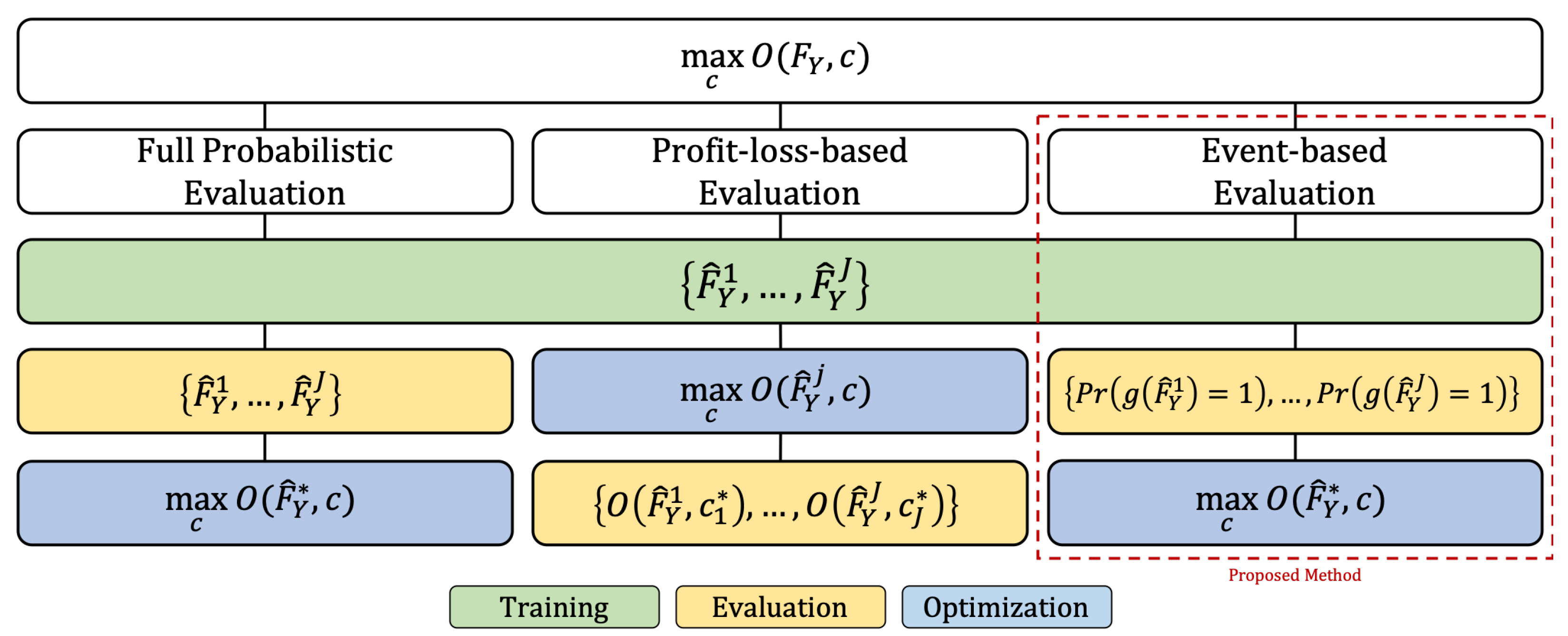
The present study considers the problem of choosing among a collection of competing forecasting models to address a stochastic decision-making problem such as:
where Y, with multivariate distribution function , represents the source of uncertainty, and c denotes the variables to be optimized. Figure 1 summarizes the considered forecast evaluation approaches. Given a collection of forecasts , the forecast user can fully evaluate each individual model using and use the best model’s forecast to solve (full probabilistic evaluation). Alternatively, the optimization problem can be solved for each forecast , and the resulting collection of objectives is used to evaluate the forecasting models (profit–loss-based evaluation). The first approach has two deficiencies. First, the reliable evaluation of a multivariate distribution forecast constitutes a challenging problem in its own right. Second, the approach may involve the implicit assessment of a model’s ability to capture a characteristic of the distribution irrelevant to the optimization problem at hand. Yet, apart from being computationally expensive, the second approach does not involve the direct evaluation of the distribution forecasts. Consequently, the present paper considers a third approach (event-based evaluation). An event that captures the relevant characteristic of the distribution is defined, where the event constitutes a mapping from the support of the multivariate distribution to a binary outcome. The probability of the event’s occurrence is derived, and the evaluation of the collection of probability forecasts allows for the identification of to solve . Two exemplary profit-maximization problems motivated by the daily operation of a risk-neutral energy trading company are considered, a pumped-hydro storage plant problem and a renewable energy trading problem. We apply a probabilistic forecasting scheme using ensemble forecasts and evaluate them by the aforementioned approaches.
Event-based evaluation of multivariate forecasts is not completely new to the forecasting literature. It has been originally proposed in the field of meteorology and applied to wind power generation forecasts (e.g., [23]). To facilitate comparison between the full probabilistic and event-based approaches for electricity price ensemble forecasts, we also consider whether the proposed event-based evaluation more reliably identifies the forecasting model that is to be preferred from an economic perspective. To this end, we use the ensemble forecasts to solve the stochastic decision-making problems and study the generator’s profit loss introduced by [19]. Note that profit–loss-based evaluation constitutes an approach in its own right (e.g., [24]) but is computationally expensive, as it requires the solution of the underlying stochastic optimization problem, and only serves as a means of comparison between the full probabilistic and event-based approach here.
The contributions of the present paper to the literature are the following.
- We introduce an event-based evaluation framework for electricity price ensemble forecasts.
- By deriving the considered events directly from the stochastic decision-making problems, we bridge the gap between the strands of the literature concerned with full probabilistic forecast evaluation and the economic consequences of forecast utilization.
- Our event-based evaluation framework is applicable to any stochastic optimization problem, where uncertainty is captured through ensembles, and thus combines the advantages of standard probabilistic evaluation and prescriptive analytics.
- We provide empirical evidence that the event-based evaluation framework more reliably identifies the economically equivalent electricity price forecasting models.
It is not the purpose of the paper to present new algorithms for electricity price ensemble forecast generation. We base the exposition of the proposed evaluation framework on state-of-the-art econometric models, but other approaches such as generative adversarial networks or MCMC methods are equally conceivable. Irrespective of the chosen approach, the features of electricity prices such as autoregressive effects, calendar effects, time-varying volatility, etc., should be captured by the underlying EPF model (see [25] (Section 3.4.2)).
The remainder of the paper is organized as follows: In Section 2, we present the stochastic decision-making problems and derive the associated events that capture the underlying characteristic of interest to the forecast user. Section 3 introduces the econometric models, whereas the proposed event-based evaluation framework is presented in Section 4. The results are presented and discussed in Section 5. Section 6 concludes, and a nomenclature is provided thereafter.
2. Decision-Making Problems and Event Probability Forecasts
To address a particular stochastic decision-making problem, a forecast user may have to choose among a collection of competing electricity price forecasting models. Depending on the payoff structure of the decision-making problem, the forecast user is implicitly interested in a specific characteristic of the underlying price distribution and would like to choose the forecasting model that best replicates this particular feature of the data generating process. We propose an event-based evaluation framework to assess a forecasting model’s ability to capture the characteristic of interest, where an event constitutes a mapping from the support of the multivariate price distribution to a binary outcome. The event definitions are based on the underlying decision-making problems and thus directly capture the characteristic of interest. It should be noted that the probability of the event’s occurrence can be calculated from the multivariate price distribution. Thus, a forecasting model’s ability to predict the probability of the occurrence of the event is directly linked to its ability to replicate the feature the forecast user is implicitly interested in. In the present study, all forecasts are communicated in the form of electricity price ensemble forecasts. Given an ensemble forecast, each day-ahead price path is mapped to an indicator variable, which takes a value of one if prices along the path are such that the specific event occurs. The day-ahead probability forecast for the binary event implied by the ensemble is given by the relative frequency of the event’s occurrence across the collection of simulated paths. Note that we denote by the price in hour h on day t, whereas denotes the entire price path on day t, i.e., .
2.1. Pumped-Hydro Storage Plant Event
The optimal operation of a pumped-hydro storage plant for time spread arbitrage constitutes the first decision-making problem. An RES-based energy system is associated with increased importance of storage and flexibility options. Pumped-hydro storage plants constitute such a flexibility option and have thus received considerable attention in the literature (e.g., [26,27]). Ref. [26] maintains that the traditional modus operandi in thermal dominated electricity markets has been to pump at night and to turbine around noon. However, the economic rationale for pumped-hydro storage plants has been undermined by the success of Photovoltaic (PV) generation in particular, as this has largely suppressed peak electricity prices around noon. It is thus of importance for operators of pumped-hydro storage plants to assess whether the asset’s operation will be profitable in the day-ahead market. The optimization problem considered in this study is based on [26] but constitutes the discrete scenario-based version of it. The following equations describe the problem.
It is assumed that the reservoir is filled with at , and the expected profits from operation of the pumped-hydro storage plant (2) are optimized subject to the set of constraints. represents the electricity price in hour h of day t associated with electricity price scenario path m, which has a probability of occurring. Equation (3) ensures that the change in the fill level of the reservoir is equal to the sum of turbining and pumping , accounting for the efficiency factor . Constraints (4)–(6) ensure that the control variables remain within the possible ranges. Since we are considering the profitability of the time spread arbitrage, the fill level of the reservoir cannot fall below the fill level at the beginning of the optimization period (8). The preceding thus constitutes a simplified yet adequate representation of a pumped-hydro storage optimization problem. Advanced formulations of the problem, more representative of the underlying technical installation of the plant, can be found in [27,28], for example. Following [26], we consider a pumped-hydro storage with pumping and turbining capacity of 200 MW ( and ), a maximum storage level of 1000 MWh () and a starting storage level of 500 MWh (). is assumed to be 0.7.
For any given day-ahead price path , the necessary condition for a profitable operation of the pumped-hydro storage plant is given by , where and represent the minimum and maximum prices on day , respectively (e.g., [26]). The event associated with the considered pumped-hydro storage optimization problem is therefore that the efficiency condition is met, and the probability of occurrence implied by an ensemble forecast is defined as:
where and denote the minimum and maximum price along ensemble path m for day , respectively. The event is referred to as “pump event” in the remainder of the paper.
2.2. Six Hours of Negative Electricity Prices Event
The optimal trading of an energy trading company under the German Renewable Energy Sources Act constitutes the second decision-making problem. Increasing intermittent RES capacity in combination with the conventional generation of limited flexibility has raised the likelihood of negative electricity prices. These negative prices reduce the market reference value of RES generation and subsequently increase the pay-out under the German renewable subsidy scheme. Yet, the German Renewable Energy Sources Act (§51 EEG 2017) stipulates that subsidy payments to RES are retrospectively withheld in case of six or more consecutive hours with negative electricity prices, as negative prices indicate that there is excess production and there is no economic or environmental benefit perceived in subsidizing excess production. Operators and energy traders are therefore incentivized to cut infeed in these hours and do have an incentive to correctly forecast the occurrence of six or more consecutive negative electricity prices. The considered energy trader owns a wind power plant that falls under the German subsidy scheme and must decide whether to sell the electricity on the day-ahead or the intraday market. Additionally, the plant can also be shut down. The following equations describe the energy trader’s optimization problem.
The energy trader maximizes their expected profits (10) deciding on the share of production to sell on the day-ahead market () and to sell on the intraday market (). represents the day-ahead electricity price in hour h of day t associated with electricity price scenario path m, and denotes the associated price on the intraday market. The probability of scenario path m occurring is . If the considered hour does not belong to a block of six or more consecutive hours of negative prices () the trader also receives a subsidy (EUR/MWh). Yet, if the considered hour is part of a block of six or more consecutive hours of negative prices, no subsidy is paid. Constraints (11)–(13) ensure that the individual shares of production lie between zero and one and do not sum to more than one. It should be noted that we intentionally abstract away from wind power forecasting errors and assume that denotes both the wind power production forecast and the respective realized production. We consider a wind power plant with a capacity of 5 MW that is paid equal to the difference between the plant’s guaranteed remuneration and the monthly German reference market value as published by the German Transmission System Operators (TSOs). Thus, is constant over all hours h and days t of a given month. The hourly production of the wind power plant is obtained by scaling down historical German wind onshore production to an installed capacity of 5 MW.
The event associated with the optimal trading problem is the occurrence of six or more consecutive hours of negative prices. Let denote a function that maps a given price path to , depending on whether such a block of negative prices is realized. The probability of occurrence implied by an ensemble forecast is defined as:
where represents ensemble price path m for day . The event is referred to as the “6h-negative event” in the remainder of the paper.
3. Electricity Price Ensemble Forecasts
The electricity price ensemble forecasts are based on two well-documented models from the literature. In the naive model, the electricity price of a particular hour h on day t is equal to the price of the same hour the week before, if t constitutes a Monday, Saturday or Sunday, or it is equal to the price of the same hour the day before for all other days (e.g., [29,30]). Recall that constitutes one element of the entire price path .
The second model belongs to the class of so-called expert models and is directly taken from [31]. It characterizes the electricity price of a particular hour h on day t as a function of autoregressive terms, non-linear terms, the price of the last hour of the preceding day and dummy variables that capture calendar information. Note that we deliberately do not capture all of the features presented in [25], using this model.
We estimate the parameters of the expert model using the Ordinary Least Squares (OLS) estimator (mean regression) and the Quantile Regression (QR) estimator with (median regression). Additionally, a Support Vector Regression (SVR) with the same explanatory variables is considered. The hyperparameters of the SVR are selected using the analytic approach of [32]. Thus, the presented results of the SVR could be further improved by careful tuning of the hyperparameters, which is beyond the scope of the present work. It should be noted that the parameters of the forecasting models are recalibrated at every timestep over the out-of-sample period.
The hourly day-ahead price forecasts are calculated from each individual model and random disturbances are added to generate an ensemble of simulated hourly day-ahead price paths. The present study considers two approaches to generate said disturbances. They are either drawn from a multivariate Student’s t-distribution, which has been fitted to the sample of residuals, or derived using residual-based bootstrapping. It should be noted that we fit both a multivariate Student’s t-distribution as well as a multivariate normal distribution, as the limiting case of the former, to the residuals. We subsequently consider whichever achieves the higher likelihood and refer to it as multivariate Student’s t-distribution. The non-parametric bootstrapping algorithm is also multivariate in the sense that it returns a vector of 24 residuals of a particular day to preserve the intraday correlation structure. The various combinations of econometric models, estimation techniques and simulation approaches provide eight different specifications, the details of which are summarized in Table 1. Note that corresponding ensemble forecasts of intraday electricity prices are required to address the optimal trading problem of the energy trading company. They are generated from the day-ahead forecast ensembles by adding random disturbances bootstrapped from a sample of historical deviations between day-ahead and corresponding intraday prices. The probability predictions implied by each ensemble forecast are subsequently derived as outlined above.
4. Forecast Evaluation
The predicted electricity prices are communicated in the form of ensemble forecasts, that is, a collection of M possible day-ahead electricity price paths. They are first evaluated using both the CRPS and the ES in combination with the DM test. Since the evaluation is based on the price forecasts directly, the approach is referred to as the full probabilistic approach. The probability of an event’s occurrence implied by an individual electricity price ensemble forecast constitutes the basis of the proposed event-based evaluation framework. Thus, the task of forecast evaluation is simplified from assessing a multivariate distribution over continuous outcomes to assessing a univariate distribution over a binary outcome. Furthermore, to facilitate comparison between the full probabilistic and event-based approach, we use the ensemble forecasts to solve the stochastic decision-making problems and study the generator’s profit loss.
Despite the simplification offered by our approach relative to the full probabilistic approach, both belong to the class of statistical evaluation approaches in the sense of relying on proper scoring rules, albeit for different underlying distributions. A limitation of our framework is thus the theoretical non-optimality of the evaluation, as it does not make use of the full informational content of the distribution forecasts. It does, however, allow us to directly link the forecasts to the decision-making problems, to which they constitute an input, and therefore extends the contemporary set of evaluation approaches.
4.1. Full Probabilistic Evaluation
For a univariate distribution forecast , the CRPS is defined as:
where denotes the price realization. denotes a random variable with distribution and is an i.i.d. copy of .
Similarly, for a multivariate distribution forecast the ES is defined as:
where denotes the price path realization. denotes a multivariate random variable with distribution and is an i.i.d. copy of . represents the norm. Note that, in the context of the present paper, the expected values are estimated by the respective sample means and that the values for , , and are taken from the ensemble forecasts (see [18] for further details).
To establish conclusions on statistically significant deviations in forecasting accuracy between any two models, as indicated by differences in their CRPS and ES, the DM test is applied (e.g., [31,33]). Given the score values of models A and B, namely, and , the loss differential series is defined as , where denotes the norm. The DM test allows considering whether the expected value of the loss differential series is zero, which is indicative of the forecasts from both models being equally accurate. We test the one-sided null hypothesis and report the p-values for all pairwise comparisons between the forecasting models. If the null hypothesis of the test for models A and B is rejected, it is concluded that the forecasts of model B are significantly more accurate.
4.2. Event-Based Evaluation
A series of implied day-ahead probability forecasts is derived for each ensemble forecast. In addition, the corresponding event indicator series is observed. To evaluate forecasting accuracy, one may compare the predicted probabilities with the realizations of the event. The average of the squared deviations over the out-of-sample period lends the Quadratic Probability Score (QPS). Further insights on the deficiencies of the considered forecasting models can be obtained using the decompositions of the score. The QPS-based approach is, however, not well suited for the evaluation of probability predictions for rare events. To reliably evaluate probability predictions of rare events, techniques developed for the evaluation of binary classifiers are also considered.
The QPS is defined as the expected value of the squared deviation between probability forecast (see (9) and (14)) and realization . The expected value is again estimated by the sample mean.
The QPS constitutes a proper, negatively oriented score that takes values between zero and one, where zero denotes perfect forecast accuracy. Since it evaluates accuracy over the entire range of probabilities, the QPS is a global measure of forecast accuracy. Again, the DM test is used to establish statistically significant deviations between the QPS values of any two models.
An understanding of the deficiencies of the considered forecasting models can be obtained through a decomposition of the QPS. The Murphy Decomposition (MD) gives the QPS as sum of three terms:
It should be noted that the formulation above is due to [34]. The MD requires the evaluation of conditional means of the event indicator series given the forecasts. To this end, one can assign them to J predefined bins of probability, but the effect of binning needs to be accounted for in the derivation of the MD (e.g., [34]). The Uncertainty (UNC) term represents the uncertainty a forecaster faces when issuing the forecast. It is given by the variance of the event indicator series , which is unobserved at the time of forecast issuance. The notion of Calibration (CAL), captured by the second term, represents the correspondence between conditional mean observation and conditioning forecast; that is, the correspondence between the mean of the event indicator series and forecasts within a particular bin. Any deviation from perfect calibration (CAL = 0) increases the QPS above uncertainty and is referred to as the level of miscalibration. On the contrary, Generalized Resolution (GRESO), the third term, reduces the QPS. Its first component represents the relation between the conditional mean observation and the unconditional mean observation, that is, how well a particular forecasting model distinguishes a particular probability case from relative frequency and attaches different probabilities to different realizations. Following [34], we combine this component with two within-bin terms that adjust the MD for the effect of binning. The present study considers two approaches to binning, both of which lend a series of partitions of the unit interval with the number of subintervals ranging from 1 to 10. The first approach simply divides the unit interval into the specified number of subintervals of equal size. The second approach utilizes a slightly altered version of the constrained k-means algorithm of [35]. It clusters the probability predictions of all models for a particular event, but the constraint set is such that at least five observations of each model fall within each cluster. The bin boundaries are derived from the respective midpoints between the cluster centroids. We find that, when using the binning-robust form of the MD, the differences between the decompositions under the two binning approaches are negligible. Some gains in accuracy are uncovered for constrained k-means binning when the non-robust decomposition is used, but our results are unaffected.
The equal weighting scheme employed in the calculation of the QPS implies that it does not distinguish between the frequent and nonfrequent realization of an event. Yet, when forecasting probabilities of a rare event, an event that occurs on less than five per cent of forecasting occasions (e.g., [36]), then regularly predicting its non-occurrence correctly will lead to a low QPS, despite a potential failure to predict its occurrence, which may be of primary interest. Consequently, the QPS-based approach is not ideal for the evaluation of rare event probability forecasts, as the influence of the frequent realization on the evaluation measure should be minimized. To this end, one can consider the techniques for the evaluation of binary classifiers.
A discrete classifier for a binary outcome is a model that directly predicts an event’s occurrence or non-occurrence rather than probabilities of occurrence. The accuracy of said classifier over the out-of-sample test set can be summarized in a so-called contingency table, which illustrates the correspondence between forecasts and realizations (cf. Table 2).
To analyze the performance of the discrete classifier, define the True Positive Rate (TPR) and False Positive Rate (FPR), which denotes the proportion of observations where the event was predicted and did occur (TPR = ) and the proportion of observations where it was predicted but did not occur (FPR = ), respectively. One can subsequently plot the FPR against the TPR in a two-dimensional space, referred to as Receiver Operating Characteristic (ROC) space. A discrete classifier is represented by a single point in the ROC space with the point of optimality given by . By focusing solely on the cases, where the event was forecast to realize, it constitutes a better approach for the evaluation of a rare event’s probability predictions, especially when its occurrence is of primary concern to the forecast user.
The approach, however, requires the forecasts from a probabilistic classifier to be transformed to discrete forecasts, taking values of zero or one. Said transformation can be achieved by specifying a probability threshold, where the event is predicted when a probability lies above it. By varying the threshold, one can trace out the ROC curve of a probabilistic classifier. ROC curves themselves constitute a tool of classifier evaluation and exhibit the nice property of being invariant to class distribution. Yet, although it is possible to compare prediction models on the basis of their corresponding ROC curves, it is more common to calculate the Area under Receiver Operating Characteristic Curve (AUROC) as a scalar measure of aggregate performance. Since the AUROC always constitutes a subarea of the unit square, it lies strictly between 0 and 1.
One established shortcoming is that ROC curves may cross, implying that one curve and hence one model may exhibit a larger AUROC, although the alternative model may exhibit a better performance, as indicated by a higher ROC curve, over the majority of the range of classification thresholds. Ref. [37] derives another fundamental deficiency of the AUROC as measure of forecasting performance. It shows that a comparison of AUROC values amounts to comparing the forecasting models using metrics that themselves depend on the models, essentially meaning that the comparison uses a different metric per model. To address said problem of evaluation, Ref. [37] proposes the so-called H-Measure, which the present study reports alongside the AUROC to evaluate forecasting accuracy for rare events.
4.3. Profit–Loss-Based Evaluation
To compare the priced-based and event-based approach for electricity price forecast ensembles, we consider whether the event-based evaluation more reliably identifies the forecasting model that is to be preferred from an economic perspective. The ensemble forecasts are used to solve the stochastic decision-making problems, and the electricity trader’s profit loss as introduced by [19] is studied.
The profit loss associated with forecasting model A is the difference between profit under perfect foresight, that is, knowing the actual realized price path of day t and the profit achieved from basing all decisions on the forecast ensemble of forecasting model A. It is defined as:
where the realized profit is a function of both the realized price path and the individual paths of the ensemble forecast . The DM test can also be considered by defining the loss differential series based on profit loss, i.e., .
5. Empirical Results and Discussion
To illustrate the applicability of the proposed event-based evaluation framework for electricity price ensemble forecasts, we conduct an out-of-sample forecasting study on German day-ahead electricity prices. The considered sample ranges from 1 January 2016 to 31 December 2019 with the last 730 days being used as an out-of-sample test set.
For each day of the out-of-sample test set and each model specification in Table 1, an electricity price ensemble forecast consisting of 1000 paths of 24 electricity prices is generated using a rolling window of 731 days. The ensemble forecast constitutes the predicted multivariate day-ahead price distribution, which is first evaluated using the full probabilistic approach. Each ensemble forecast is subsequently used to calculate the profit loss by solving the stochastic decision-making problems and to derive the implied probability of the associated events’ occurrence. These constitute the basis for the aforementioned profit–loss-based and event-based forecast evaluation. The forecasting study is performed on a MacBook Pro with 2 cores, a 2.7 GHz processor as well as 16 GB RAM, and the execution times for the individual tasks are reported in Table 3. Whereas the generation of ensemble forecasts exhibits the longest execution time, the reported results underscore the much higher computational cost of profit–loss-based evaluation relative to both full probabilistic and event-based evaluation.
The results of the full probabilistic evaluation of the ensemble forecasts are shown in Table 4, where we report the average of both the CRPS and the ES over the out-of-sample period. Note that each of the reported Table 4, Table 5, Table 6, Table 7 and Table 8 is directly linked to one of the forecast evaluation approaches summarized in Figure 1. In Table 4, one can observe that the expert-based specifications (Ex-B, QREx-B, SVREx-B, Ex-t, QREx-t and SVREx-t) outperform the naive specifications (N-B and N-t), whereas the SVR-based models outperform the mean- and median-regression models. In addition, the bootstrapped-based specifications exhibit marginally lower scores than the t-based specifications among the expert models. SVREx-B constitutes the best overall model and has a slightly lower CRPS and ES values than SVREx-t.
In Figure 2, we summarize the results of all considered DM tests. In each of the six panels, a square displays the p-value of a pairwise test of equal predictive performance against the alternative hypothesis that the model in the row predicts significantly less accurately than the model in the corresponding column. White squares indicate that no significant difference in forecasting performance can be uncovered, whereas green squares indicate significant deviations in forecasting performance at the 10, 5 and 1 per cent levels of significance, with lighter green implying a more significant difference.
The results of the CRPS-based and ES-based DM tests are shown in the first row of Figure 2 and confirm the preceding discussion based on Table 4. All expert models exhibit significantly lower scores than the naive models, as do the SVR-based models in comparison to the mean- and median-regression models. Yet, the overall best model (SVREx-B) does not significantly outperform the second-best model (SVREx-t). Interestingly, the conclusions for the pairwise DM tests based on either the CRPS or ES are identical, lending support to the literature’s approach to average univariate scores of marginal distributions to assess multivariate distribution forecasts.
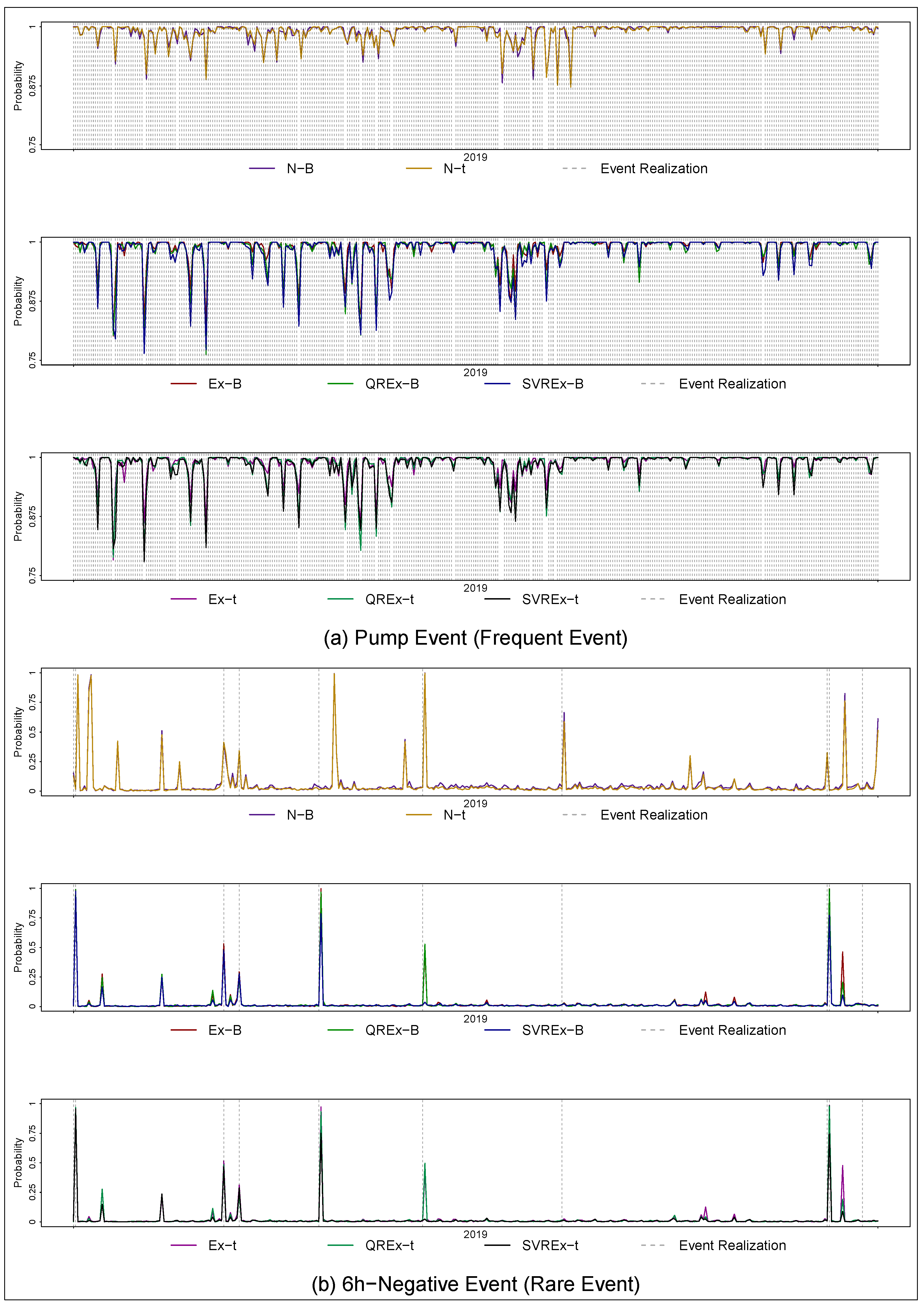
The present study proposes an event-based evaluation framework for electricity price ensemble forecasts, the basis of which are the implied probabilities of occurrence of a binary event associated with the stochastic decision-making problems. The time series of the implied day-ahead probabilities across events and models for 2019 are displayed in Figure 3. The colored lines trace out the implied probabilities, whereas the dashed grey vertical lines indicate the realization of the respective event. Clearly, the considered pump event constitutes a rather common event in 2019. On the contrary, the 6h-negative event rarely realized. In fact, with 15 occurrences over the out-of-sample period, it falls within the rare event definition of [36]. Figure 3 indicates that the predicted probabilities vary both across time and models. For example, the specifications based on the naive electricity price model structurally assign higher probabilities to the occurrence of the pump event over the year. Similarly, the expert-based specifications assign much lower probabilities to six consecutive hours of negative prices than the naive-based specifications. In addition, it seems that the models predict the realization of the rare event rather well, which is, however, misleading. Closer inspection reveals that the realization of the rare event is predicted for the day after its occurrence, the reason being that the prices, which are such that the event occurs, subsequently form the basis for the day-ahead prediction and thus assign a high probability to the event’s occurrence.
The QPS values are reported in Table 5, and the corresponding results of the QPS-based DM test are shown in the second row of Figure 2. It should be noted that the expert-based specifications exhibit significantly lower QPS values than the naive specifications for both events. For the pump event, the QR-based specifications achieve lower QPS values than the remaining expert-based specifications. QREx-t constitutes the overall best model and has a slightly lower QPS than QREx-B and SVREx-B. Yet, the results of the DM test show that QREx-t does not statistically significantly outperform them, whereas it does for all other considered specifications. Similarly, QREx-B fails to significantly outperform both SVR-based models. We find the overall level of the QPS to be lower for the 6h-negative event than for the pump event, which illustrates the influence of the frequent realization of the rare event on the evaluation measure. Since the models generally assign low probabilities to the day-ahead occurrence of the event, their respective scores are low. SVREx-B constitutes the overall best model, but no significant difference in predictive performance can be uncovered for the SVR-based models in comparison to the QR-based models.
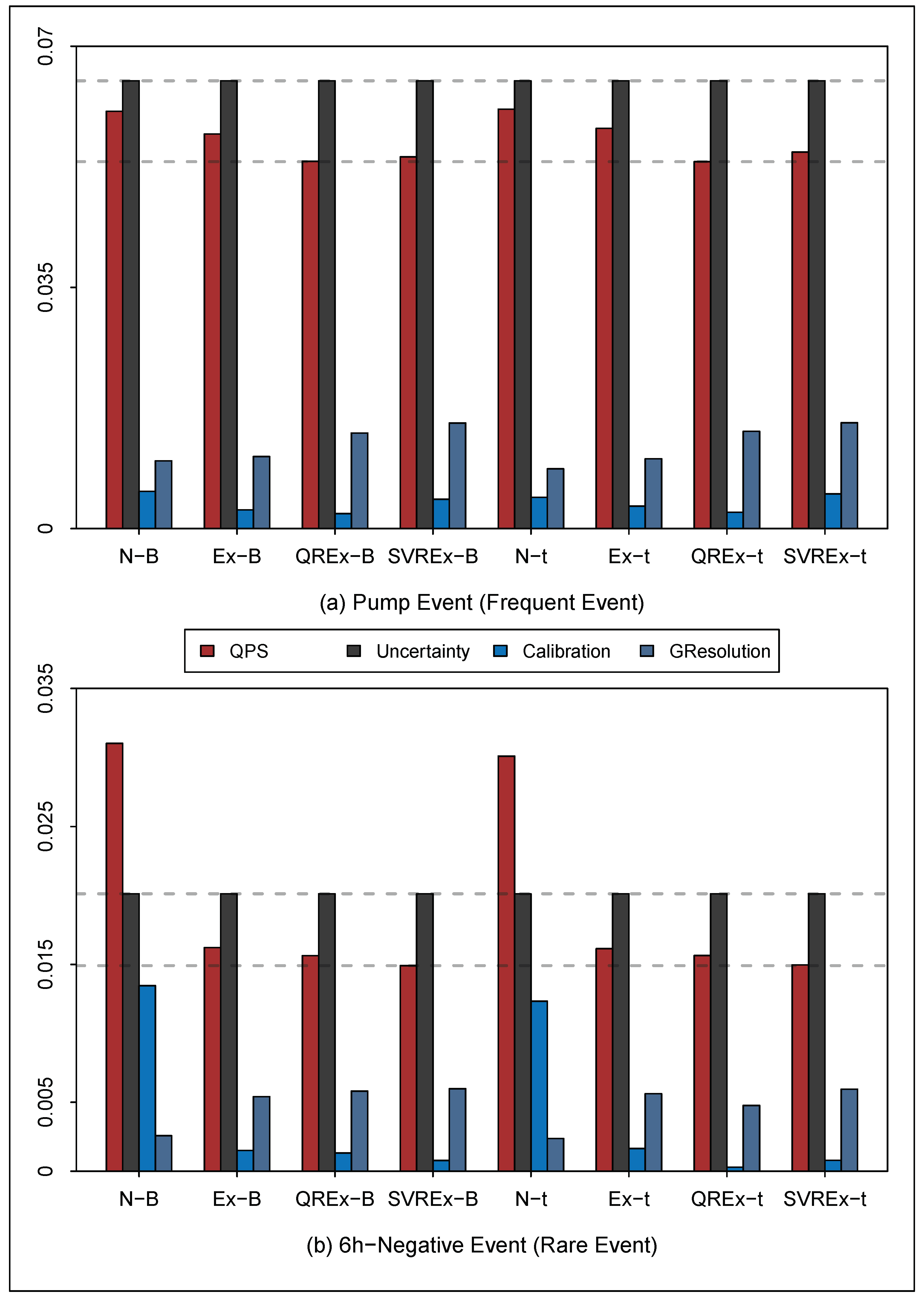
The MD provides further insights into the deficiencies of the considered forecasting models. Figure 4 shows the QPS and its respective components from the MD for both events. It should be noted that the uncertainty component, being derived from the event indicator series over the out-of-sample period, is the same across all models for a given event. For the pump event, all considered specifications succeed in reducing uncertainty. In addition, the SVR-based and QR-based models achieve higher generalized resolution than all other models, implying that they are more able to distinguish between the respective cases of the event. As the QR-based models exhibit the lowest level of miscalibration, they achieve the lowest QPS values overall. Interestingly, the SVR-based models achieve higher levels of generalized resolution but only at the cost of higher miscalibration. For the 6h-negative event, we find that the naive specifications increase the QPS above uncertainty, due to substantial miscalibration. Conversely, the expert-based specifications succeed in reducing the uncertainty. Within that class, the SVR-based models together with QREx-t are the least miscalibrated with slightly higher generalized resolutions, implying that, overall, the issued forecasts correspond well with the realization of the event and that the models are most effective in using the provided information to distinguish cases of occurrence and non-occurrence of the event.
In contrast to the QPS, both the AUROC and the H-Measure are positively oriented measures of forecasting accuracy, focusing on the event’s occurrence. The respective values per model are provided in Table 6 and Table 7. It should be noted that all AUROC values are larger than 0.5, implying that all models perform better than random class guessing. For both events, the naive specifications exhibit the lowest AUROC and H-Measure among all considered models, underscoring the results derived from the QPS comparisons. For the pump event, the SVR-based models exhibit the highest AUROC, whereas SVREx-t and QREx-t exhibit the highest H-Measure. The results are thus somewhat different to the results based on the QPS, where both QR-based models perform best. Yet, the pairwise DM tests show that the QR-based models fail to significantly outperfom at least one of the SVR-based models, and thus the SVREx-t model simply predicts the event’s occurrence more reliably. For the 6h-negative event, Ex-B achieves both the highest AUROC and H-Measure values with SVREx-B and QREx-B constituting the respective second-best models. In addition, each specification with bootstrap-based simulation outperforms its t-distribution-based simulation counterpart. This constitutes a surprising result, given that Ex-B exhibits the highest QPS among the expert-based specifications. It suggests that an evaluation procedure that fails to account for the frequent realization provides misleading conclusions when forecasting probabilities for rare events. In particular, the finding suggests that Ex-B exhibits a higher QPS value overall, as it structurally assigns higher probabilities to the occurrence of the rare event (see lower panel of Figure 3) but that it also exhibits a higher hit rate when the event actually occurs.
To compare the full probabilistic and event-based evaluation approach and to assess whether one is to be preferred by the forecast user, the forecast models are also evaluated based on profit loss. The profit loss values are reported in Table 8, and the corresponding results of the profit–loss-based DM tests are shown in the third row of Figure 2. For the pump event, the profit loss is higher for the naive models, whereas it is minimized by using the forecasts from SVREx-B and QREx-B. Yet, considering the DM test results, one finds that SVREx-B does not significantly outperform QREx-B and SVREx-t, which exhibits the highest AUROC and H-Measure. Similarly, for the 6h-negative event, the results for profit loss are comparable to the results based on the H-Measure. QREx-B and Ex-B achieve the lowest profit loss and the pairwise DM tests uncover that both significantly outperform at least one SVR-based models. Overall, considerably fewer significant outperformances can be established based on profit loss, and the significant differences in quality between the SVR-based models and the remaining expert-based models are striking. The correct prediction of an occurrence of six consecutive hours of negative electricity prices has a positive impact on the profitability of the energy trader, even if the considered model overpredicts the occurrence of the event. Consequently, QREx-B and Ex-B, being the models that predict the event’s occurrence most reliably, also constitute the models with the lowest profit loss.
For the considered sample of German electricity prices, neither the event-based approach nor the profit–loss-based approach establishes the statistically significant differences in forecasting performance for the SVR-based models suggested by the full probabilistic approach. The QR-based models are not clearly outperformed under the event-based and the profit–loss-based approach for the pump event. The same result is established for the 6h-negative event based on the QPS, whereas the evaluation techniques for binary classifiers and the profit–loss-based approach establish Ex-B as the best-performing model. Thus, the event-based approach does not suggest statistically significant differences in forecasting performance that are not in line with the economics of the stochastic decision-making problems to which the forecasts constitute an input. The same holds for the profit–loss-based approach, but that approach comes at a considerably higher computational costs. As the event-based approach more reliably identifies the economically equivalent models for the studied decision-making problems, it extends the prevailing full probabilistic approach. Yet, the conclusions are specifically established for an energy trader operating in the German market. We leave the confirmation of the presented results for additional decision-making problems under different price regimes to future work. In addition, the results suggest that for decision-making problems linked to rare events, an event-based evaluation with techniques that focus on the occurrence of the event is beneficial to an event-based evaluation with techniques strongly influenced by the frequent realization of the event.
6. Conclusions
The present paper considers the problem of choosing among a collection of competing electricity price forecasting models to address two stochastic decision-making problems motivated by the daily operation of a risk-neutral energy trading company. All forecasts are communicated in the form of ensemble forecasts, that is, a collection of possible day-ahead electricity price paths, which are generated from two established electricity price models in combination with a bootstrap-based and a t-distribution-based simulation approach.
The ensemble forecasts are first evaluated using the predicted prices directly. Subsequently, an event-based evaluation framework is introduced. To this end, an event per decision-making problem is defined, and the day-ahead probability forecast for the binary event implied by the ensemble is calculated and evaluated. The task of forecast evaluation is thus simplified from assessing a multivariate distribution over prices to assessing a univariate distribution over a binary outcome directly linked to the underlying stochastic decision-making problem.
While we demonstrate the applicability of the proposed event-based evaluation framework with electricity prices, it is also applicable to any stochastic optimization problem, where uncertainty is captured through ensembles (see Figure 1). It is basing the considered events directly on the stochastic decision-making problems to which the predicted distribution constitutes an input that represents the novelty of our approach. It thus combines the advantages of standard probabilistic evaluation as well as prescriptive analytics and bridges the gap between the strands of the forecasting literature concerned with full probabilistic forecast evaluation and the economic consequences of forecast utilization.
We test our event-based approach with an out-of-sample forecasting study on German day-ahead electricity prices. It is found not to uncover the statistically significant differences in forecasting performance suggested by the full probabilistic approach and therefore extends it. In addition, the results suggest that an event-based evaluation specifically tailored to the rare event is crucial for decision-making problems linked to rare events.
Author Contributions
Conceptualization, A.V. and F.Z.; methodology, A.V. and F.Z.; investigation, A.V. and F.Z.; software, A.V.; writing—original draft preparation, A.V.; writing—review and editing, F.Z. All authors have read and agreed to the published version of the manuscript.
Funding
This research received no external funding.
Institutional Review Board Statement
Not applicable.
Informed Consent Statement
Not applicable.
Data Availability Statement
The electricity price data used were purchased from EPEX Spot (https://webshop.eex-group.com/epex-spot-public-market-data accessed on 1 November 2021). The wind generation data are openly available from the German TSO Information Platform (https://www.netztransparenz.de/Erneuerbare-Energien-Gesetz/Marktpraemie/Online-Hochrechnung-Wind-Onshore accessed on 1 November 2021).
Conflicts of Interest
The authors declare no conflict of interest.
Nomenclature
| Expression | Explanation |
| Maximization Operator | |
| Objective Function | |
| c | Decision Variable |
| Y | Multivariate Random Vector |
| Cumulative Distribution Function of Vector Y | |
| Model i Forecast of | |
| Optimal Forecast of | |
| Event defined as Mapping from to | |
| Probability | |
| ∑ | Sum Operator |
| Power Price in Hour h on Day t | |
| Power Price Path on Day t | |
| Minimum Power Price on Day t | |
| Maximum Power Price on Day t | |
| m | Index of Power Price Simulation Path |
| Probability of Power Price Path m | |
| Power Price in Hour h on Day t along Path m | |
| Minimum Power Price on Day t along Path m | |
| Maximum Power Price on Day t along Path m | |
| Length of Time Interval | |
| Turbining Capacity in Hour h on Day t | |
| Generation Capacity in Hour h on Day t | |
| Efficiency Factor | |
| Maximum Turbining Capacity | |
| Maximum Generation Capacity | |
| Maximum Storage Capacity | |
| Production in Hour h on Day t | |
| Share sold on Day-Ahead Market in Hour h on Day t | |
| Share sold on Intraday Market in Hour h on Day t | |
| 6h-Negative Event Indicator for Hour h on Day t along Path m | |
| Subsidy in | |
| Dummy for Day of Week i for Day t | |
| CRPS | Continuous Ranked Probability Score |
| Expectation Operator | |
| Random Variable | |
| ES | Energy Score |
| Norm | |
| Score for Model A | |
| Score Differential for Model A and B | |
| Null Hypothesis | |
| f | Probability Forecast |
| x | Event Realization Indicator |
| QPS | Quadratic Probability Score |
| j | Index of Probability Bin |
| Mean of Event Realization Indicators | |
| Number of Probability Forecasts in Bin j | |
| Mean of Event Realization Indicators in Bin j | |
| Probability Forecast in Bin j for Day t | |
| Mean of Probability Forecasts in Bin j | |
| TPR | True Positive Rate |
| FPR | False Positive Rate |
| Profit Loss under Model A | |
| Profit under Perfect Foresight | |
| Profit under Model A Forecasts |
References
- Nowotarski, J.; Weron, R. Recent advances in electricity price forecasting: A review of probabilistic forecasting. Renew. Sustain. Energy Rev. 2018, 81, 1548–1568. [Google Scholar] [CrossRef]
- Uniejewski, B.; Marcjasz, G.; Weron, R. On the importance of the long-term seasonal component in day-ahead electricity price forecasting: Part II—Probabilistic forecasting. Energy Econ. 2019, 79, 171–182. [Google Scholar] [CrossRef] [Green Version]
- Gneiting, T.; Katzfuss, M. Probabilistic Forecasting. Annu. Rev. Stat. Its Appl. 2014, 1, 125–151. [Google Scholar] [CrossRef]
- Marcjasz, G.; Uniejewski, B.; Weron, R. Probabilistic electricity price forecasting with NARX networks: Combine point or probabilistic forecasts? Int. J. Forecast. 2020, 36, 466–479. [Google Scholar] [CrossRef]
- Weron, R.; Ziel, F. Electricity Price Forecasting. In Routledge Handbook of Energy Economics; Soytaş, U., Sari, R., Eds.; Routledge: London, UK, 2019; Chapter 35; pp. 506–521. [Google Scholar]
- Muniain, P.; Ziel, F. Probabilistic forecasting in day-ahead electricity markets: Simulating peak and off-peak prices. Int. J. Forecast. 2020, 36, 1193–1210. [Google Scholar] [CrossRef] [Green Version]
- Narajewski, M.; Ziel, F. Ensemble forecasting for intraday electricity prices: Simulating trajectories. Appl. Energy 2020, 279, 115801. [Google Scholar] [CrossRef]
- Hong, T.; Pinson, P.; Wang, Y.; Weron, R.; Yang, D.; Zareipour, H. Energy Forecasting: A Review and Outlook. IEEE Open Access J. Power Energy 2020, 7, 376–388. [Google Scholar] [CrossRef]
- Li, B.; Zhang, J. A review on the integration of probabilistic solar forecasting in power systems. Solar Energy 2020, 210, 68–86. [Google Scholar] [CrossRef]
- Li, J.; Zhou, J.; Chen, B. Review of wind power scenario generation methods for optimal operation of renewable energy systems. Appl. Energy 2020, 280, 115992. [Google Scholar] [CrossRef]
- Rachunok, B.; Staid, A.; Watson, J.P.; Woodruff, D.L. Assessment of wind power scenario creation methods for stochastic power systems operations. Appl. Energy 2020, 268, 114986. [Google Scholar] [CrossRef]
- Gneiting, T.; Balabdaoui, F.; Raftery, A.E. Probabilistic Forecasts, Calibration and Sharpness. J. R. Stat. Soc. Ser. B (Stat. Methodol.) 2007, 69, 243–268. [Google Scholar] [CrossRef] [Green Version]
- Hong, T.; Pinson, P.; Fan, S.; Zareipour, H.; Troccoli, A.; Hyndman, R.J. Probabilistic energy forecasting: Global Energy Forecasting Competition 2014 and beyond. Int. J. Forecast. 2016, 32, 896–913. [Google Scholar] [CrossRef] [Green Version]
- Jónsson, T.; Pinson, P.; Madsen, H.; Nielsen, H. Predictive Densities for Day-Ahead Electricity Prices Using Time-Adaptive Quantile Regression. Energies 2014, 7, 5523–5547. [Google Scholar] [CrossRef]
- Gneiting, T.; Stanberry, L.I.; Grimit, E.P.; Held, L.; Johnson, N.A. Assessing probabilistic forecasts of multivariate quantities, with an application to ensemble predictions of surface winds. TEST 2008, 17, 211. [Google Scholar] [CrossRef] [PubMed]
- Zhang, Y.; Wang, J.; Wang, X. Review on probabilistic forecasting of wind power generation. Renew. Sustain. Energy Rev. 2014, 32, 255–270. [Google Scholar] [CrossRef]
- Pinson, P.; Tastu, J. Discrimination Ability of the Energy Score; Technical University of Denmark: Lyngby, Denmark, 2013. [Google Scholar]
- Ziel, F.; Berk, K. Multivariate Forecasting Evaluation: On Sensitive and Strictly Proper Scoring Rules. arXiv 2019, arXiv:1910.07325. [Google Scholar]
- Delarue, E.; van den Bosch, P.; D’haeseleer, W. Effect of the accuracy of price forecasting on profit in a Price Based Unit Commitment. Electr. Power Syst. Res. 2010, 80, 1306–1313. [Google Scholar] [CrossRef]
- Zareipour, H.; Canizares, C.A.; Bhattacharya, K. Economic Impact of Electricity Market Price Forecasting Errors: A Demand-Side Analysis. IEEE Trans. Power Syst. 2010, 25, 254–262. [Google Scholar] [CrossRef]
- Mohammadi-Ivatloo, B.; Zareipour, H.; Ehsan, M.; Amjady, N. Economic impact of price forecasting inaccuracies on self-scheduling of generation companies. Electr. Power Syst. Res. 2011, 81, 617–624. [Google Scholar] [CrossRef]
- Doostmohammadi, A.; Amjady, N.; Zareipour, H. Day-Ahead Financial Loss/Gain Modeling and Prediction for a Generation Company. IEEE Trans. Power Syst. 2017, 32, 3360–3372. [Google Scholar] [CrossRef]
- Pinson, P.; Girard, R. Evaluating the quality of scenarios of short-term wind power generation. Appl. Energy 2012, 96, 12–20. [Google Scholar] [CrossRef] [Green Version]
- Ugurlu, U.; Tas, O.; Kaya, A.; Oksuz, I. The financial effect of the electricity price forecasts’ inaccuracy on a hydro-based generation company. Energies 2018, 11, 2093. [Google Scholar] [CrossRef] [Green Version]
- Petropoulos, F.; Apiletti, D.; Assimakopoulos, V.; Babai, M.Z.; Barrow, D.K.; Taieb, S.B.; Bergmeir, C.; Bessa, R.J.; Bijak, J.; Boylan, J.E.; et al. Forecasting: Theory and practice. arXiv 2021, arXiv:2012.03854. [Google Scholar]
- Steffen, B.; Weber, C. Optimal operation of pumped-hydro storage plants with continuous time-varying power prices. Eur. J. Oper. Res. 2016, 252, 308–321. [Google Scholar] [CrossRef]
- Braun, S.; Hoffmann, R. Intraday Optimization of Pumped Hydro Power Plants in the German Electricity Market. Energy Procedia 2016, 87, 45–52. [Google Scholar] [CrossRef] [Green Version]
- Finnah, B.; Gönsch, J.; Ziel, F. Integrated day-ahead and intraday self-schedule bidding for energy storage systems using approximate dynamic programming. Eur. J. Oper. Res. 2021. [Google Scholar] [CrossRef]
- Conejo, A.J.; Plazas, M.A.; Espinola, R.; Molina, A.B. Day-Ahead Electricity Price Forecasting Using the Wavelet Transform and ARIMA Models. IEEE Trans. Power Syst. 2005, 20, 1035–1042. [Google Scholar] [CrossRef]
- Conejo, A.J.; Contreras, J.; Espínola, R.; Plazas, M.A. Forecasting electricity prices for a day-ahead pool-based electric energy market. Int. J. Forecast. 2005, 21, 435–462. [Google Scholar] [CrossRef]
- Ziel, F.; Weron, R. Day-ahead electricity price forecasting with high-dimensional structures: Univariate vs. multivariate modeling frameworks. Energy Econ. 2018, 70, 396–420. [Google Scholar] [CrossRef] [Green Version]
- Cherkassky, V.; Ma, Y. Selection of Meta-parameters for Support Vector Regression. In Artificial Neural Networks—ICANN 2002; Goos, G., Hartmanis, J., van Leeuwen, J., Dorronsoro, J.R., Eds.; Lecture Notes in Computer Science; Springer: Berlin/Heidelberg, Germany, 2002; Volume 2415, pp. 687–693. [Google Scholar] [CrossRef]
- Diebold, F.X.; Mariano, R.S. Comparing Predictive Accuracy. J. Bus. Econ. Stat. 2002, 20, 134–144. [Google Scholar] [CrossRef]
- Stephenson, D.B.; Coelho, C.A.S.; Jolliffe, I.T. Two Extra Components in the Brier Score Decomposition. Weather Forecast. 2008, 23, 752–757. [Google Scholar] [CrossRef] [Green Version]
- Bradley, P.S.; Bennett, K.P.; Demiriz, A. Constrained K-Means Clustering: Microsoft Research, Redmond 20.0. Available online: http://machinelearning102.pbworks.com/f/ConstrainedKMeanstr-2000-65.pdf (accessed on 1 November 2021).
- Murphy, A.H. Probabilities, Odds and Forecasts of Rare Events. Weather Forecast. 1991, 6, 302–307. [Google Scholar] [CrossRef] [Green Version]
- Hand, D.J. Measuring classifier performance: A coherent alternative to the area under the ROC curve. Mach. Learn. 2009, 77, 103–123. [Google Scholar] [CrossRef] [Green Version]
Figure 1.
Considered Forecast Evaluation Approaches.

Figure 2.
p-Values of pairwise DM Tests: (a) CRPS-based DM Tests for Electricity Price Forecasts; (b) ES-based DM Tests for Electricity Price Forecasts; (c) QPS-based DM Tests for Pump Event; (d) QPS-based DM Tests for 6h-Negative Event; (e) Profit–Loss-based DM Tests for Pump Event; (f) Profit–Loss-based DM Tests for 6h-Negative Event.

Figure 3.
Probability Forecast and Realization Time Series for Events: (a) Probability Forecast Time Series per Model for Pump Event; (b) Probability Forecast Time Series per Model for 6h-Negative Event.
Figure 3.
Probability Forecast and Realization Time Series for Events: (a) Probability Forecast Time Series per Model for Pump Event; (b) Probability Forecast Time Series per Model for 6h-Negative Event.

Figure 4.
Murphy Decomposition for Events: (a) Murphy Decomposition Components per Model for Pump Event; (b) Murphy Decomposition Components per Model for 6h-Negative Event.
Figure 4.
Murphy Decomposition for Events: (a) Murphy Decomposition Components per Model for Pump Event; (b) Murphy Decomposition Components per Model for 6h-Negative Event.


Table 1.
Specification Overview.
| N-B | Ex-B | QREx-B | SVREx-B |
|---|---|---|---|
| Naive | Expert | Expert | Expert |
| - | OLS | QR ( = 0.5) | SVR |
| Bootstrap | Bootstrap | Bootstrap | Bootstrap |
| N-t | Ex-t | QREx-t | SVREx-t |
| Naive | Expert | Expert | Expert |
| - | OLS | QR ( = 0.5) | SVR |
| Student’s t | Student’s t | Student’s t | Student’s t |
Table 2.
Contingency Table.
| True Positives (TP) | False Positives (FP) | |
| False Negatives (FN) | True Negatives (TN) | |
| PO | NE |
Table 3.
Execution Time.
| Task | Execution Time [min] |
|---|---|
| Price Forecast and Simulation | 53.34 |
| Full Probabilistic Evaluation | 0.85 |
| Event-based Evaluation | 2.64 |
| Profit–Loss-based Evaluation | 20.11 |
Table 4.
Full Probabilistic Evaluation: Continuous Ranked Probability and Energy Score.
| Score | N-B | Ex-B | QREx-B | SVREx-B |
|---|---|---|---|---|
| CRPS | 176.56 | 118.28 | 116.47 | 115.25 |
| ES | 42.32 | 28.88 | 28.44 | 28.07 |
| Score | N-t | Ex-t | QREx-t | SVREx-t |
| CRPS | 176.76 | 118.55 | 116.73 | 115.31 |
| ES | 42.32 | 28.93 | 28.50 | 28.09 |
Table 5.
Event-based Evaluation: Quadratic Probability Score.
| Event | N-B | Ex-B | QREx-B | SVREx-B |
|---|---|---|---|---|
| Pump (Frequent) | 0.0606 | 0.0573 | 0.0533 | 0.0539 |
| 6h-Negative (Rare) | 0.0310 | 0.0162 | 0.0156 | 0.0149 |
| Event | N-t | Ex-t | QREx-t | SVREx-t |
| Pump (Frequent) | 0.0609 | 0.0581 | 0.0532 | 0.0547 |
| 6h-Negative (Rare) | 0.0301 | 0.0161 | 0.0156 | 0.0150 |
Table 6.
Event-based Evaluation: AUROC.
| Event | N-B | Ex-B | QREx-B | SVREx-B |
|---|---|---|---|---|
| Pump (Frequent) | 0.8212 | 0.8873 | 0.8851 | 0.9006 |
| 6h-Negative (Rare) | 0.7665 | 0.9076 | 0.8906 | 0.8934 |
| Event | N-t | Ex-t | QREx-t | SVREx-t |
| Pump (Frequent) | 0.8509 | 0.8788 | 0.8983 | 0.9079 |
| 6h-Negative (Rare) | 0.7533 | 0.8490 | 0.8329 | 0.8737 |
Table 7.
Event-based Evaluation: H-Measure.
| Event | N-B | Ex-B | QREx-B | SVREx-B |
|---|---|---|---|---|
| Pump (Frequent) | 0.2687 | 0.3143 | 0.3163 | 0.3379 |
| 6h-Negative (Rare) | 0.3633 | 0.6068 | 0.5822 | 0.5626 |
| Event | N-t | Ex-t | QREx-t | SVREx-t |
| Pump (Frequent) | 0.2705 | 0.3131 | 0.3622 | 0.3703 |
| 6h-Negative (Rare) | 0.3542 | 0.5045 | 0.5682 | 0.5302 |
Table 8.
Profit–loss-based Evaluation: Profit Loss.
| Event | N-B | Ex-B | QREx-B | SVREx-B |
|---|---|---|---|---|
| Pump (Frequent) | 6452 | 4081 | 3879 | 3829 |
| 6h-Negative (Rare) | 89.88 | 88.69 | 88.47 | 89.75 |
| Event | N-t | Ex-t | QREx-t | SVREx-t |
| Pump (Frequent) | 6467 | 4123 | 3944 | 3884 |
| 6h-Negative (Rare) | 89.89 | 89.19 | 88.75 | 90.22 |
Publisher’s Note: MDPI stays neutral with regard to jurisdictional claims in published maps and institutional affiliations. |
© 2021 by the authors. Licensee MDPI, Basel, Switzerland. This article is an open access article distributed under the terms and conditions of the Creative Commons Attribution (CC BY) license (https://creativecommons.org/licenses/by/4.0/).
Share and Cite
MDPI and ACS Style
Vogler, A.; Ziel, F. Event-Based Evaluation of Electricity Price Ensemble Forecasts. Forecasting 2022, 4, 51-71. https://0-doi-org.brum.beds.ac.uk/10.3390/forecast4010004
AMA Style
Vogler A, Ziel F. Event-Based Evaluation of Electricity Price Ensemble Forecasts. Forecasting. 2022; 4(1):51-71. https://0-doi-org.brum.beds.ac.uk/10.3390/forecast4010004
Chicago/Turabian StyleVogler, Arne, and Florian Ziel. 2022. "Event-Based Evaluation of Electricity Price Ensemble Forecasts" Forecasting 4, no. 1: 51-71. https://0-doi-org.brum.beds.ac.uk/10.3390/forecast4010004