
Analysing Historical and Modelling Future Soil Temperature at Kuujjuaq, Quebec (Canada): Implications on Aviation Infrastructure


Abstract
:1. Introduction
- (1)
- To assess temporal trends of the historical soil temperature record of Kuujjuaq, Quebec and their relationship to concurrent air temperature;
- (2)
- Deploy a novel approach by using statistical downscaling to develop a robust relationship between soil temperatures and a range of atmospheric variables;
- (3)
- Using the relationships developed to project soil temperatures at Kuujjuaq from 1997 to 2086.
2. Materials and Methods
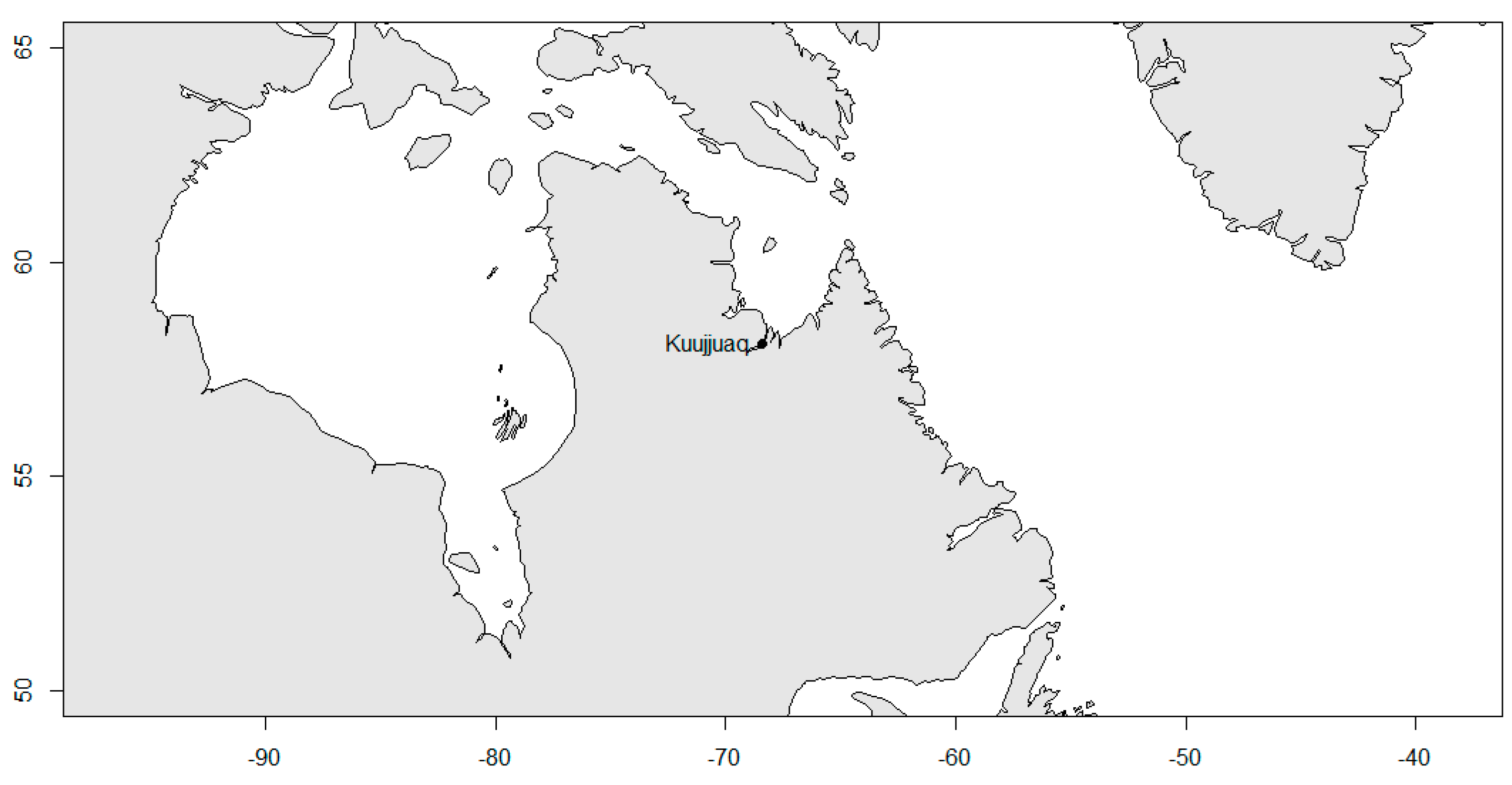
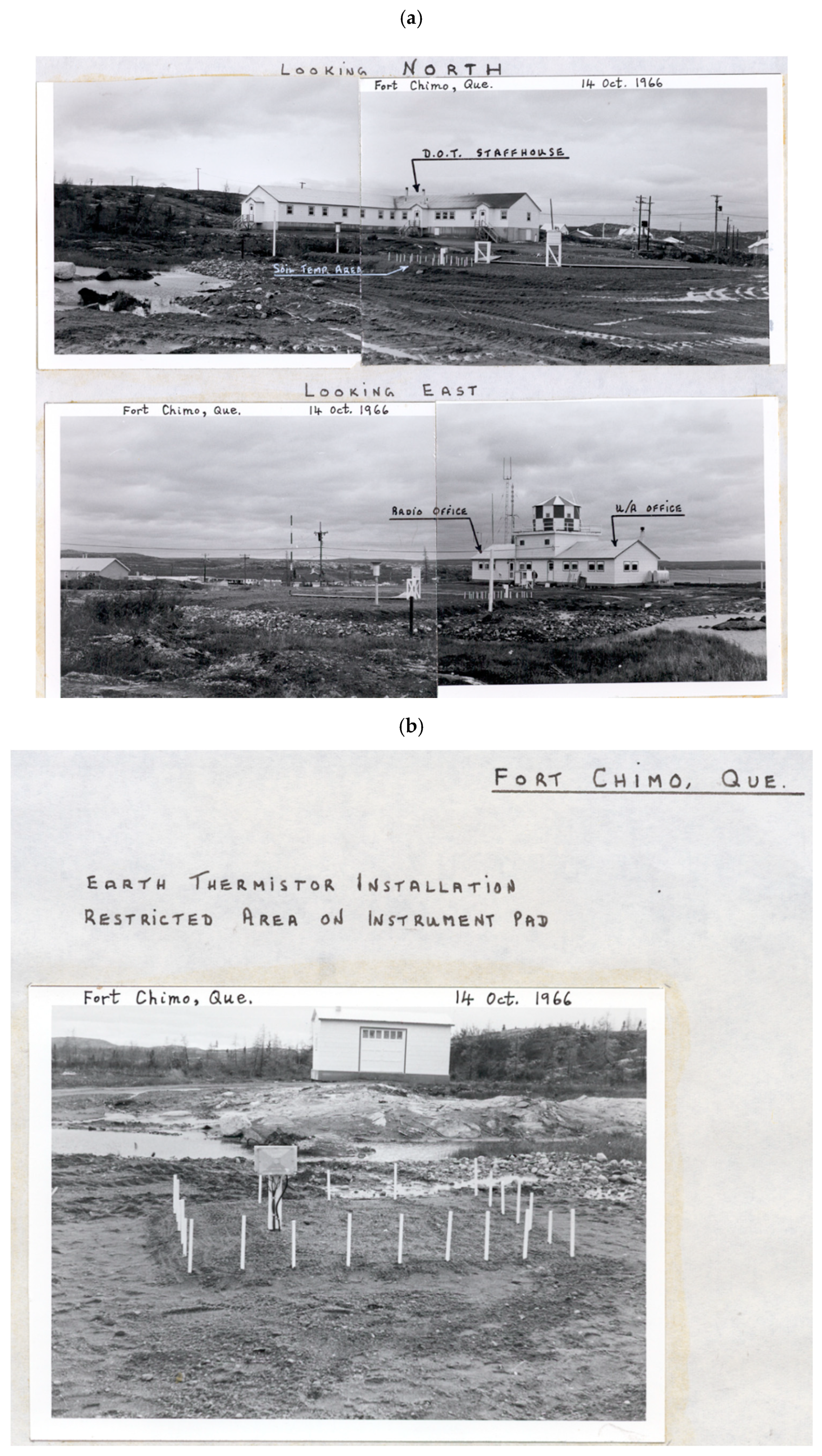
2.1. Site Characteristics
2.2. Data Collection
2.3. Historical Data Analysis
2.4. Statistical Downscaling
2.5. Climate Projections
Assumptions
3. Results
3.1. Historical Analysis
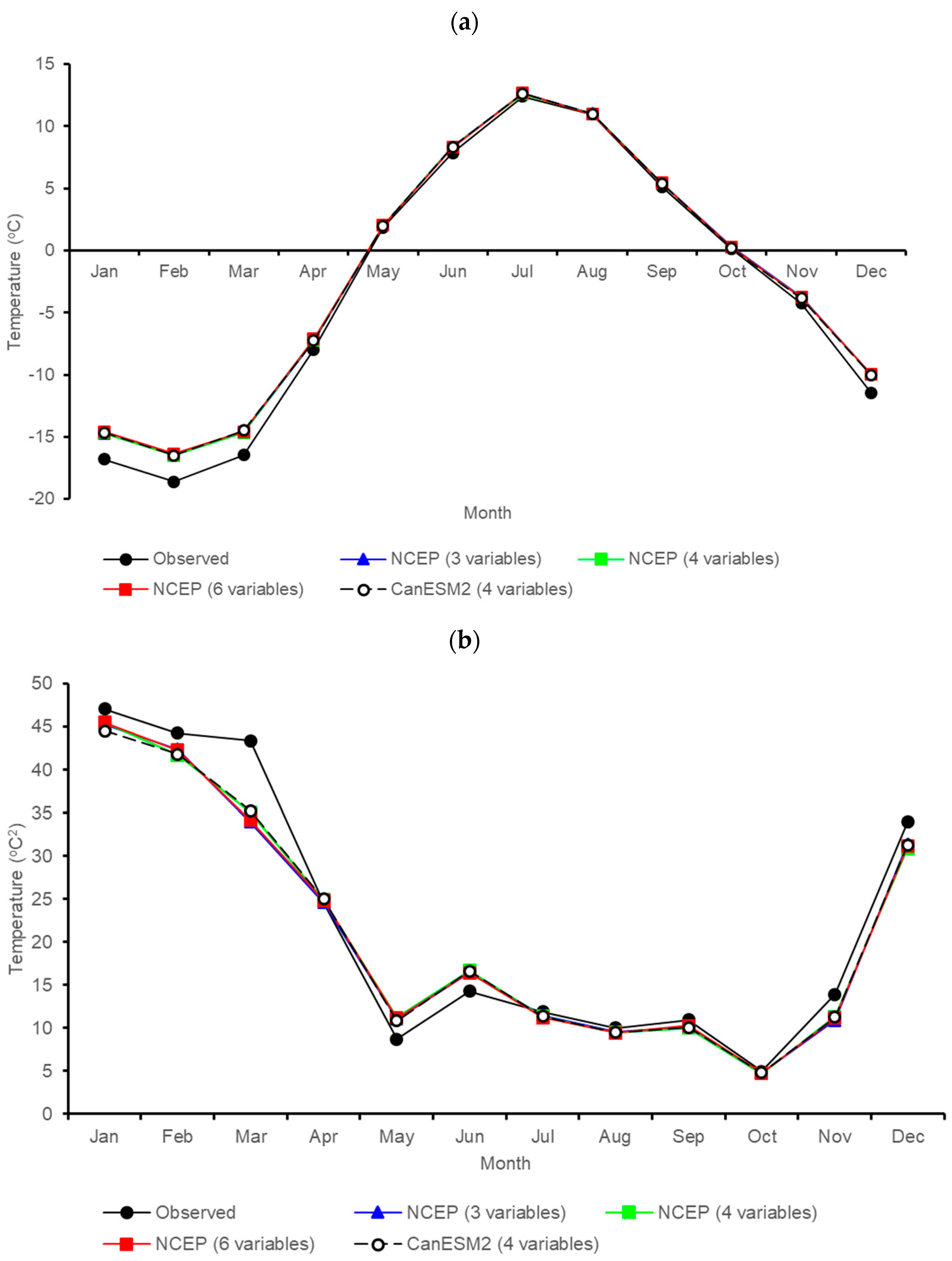
3.2. Statistical Downscaling
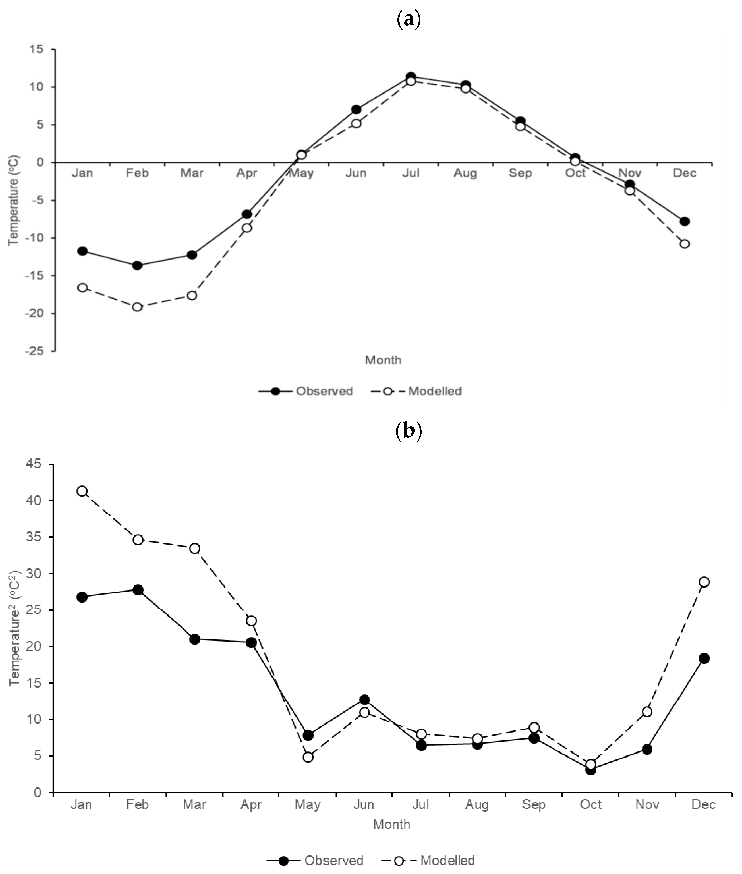
3.3. Projections
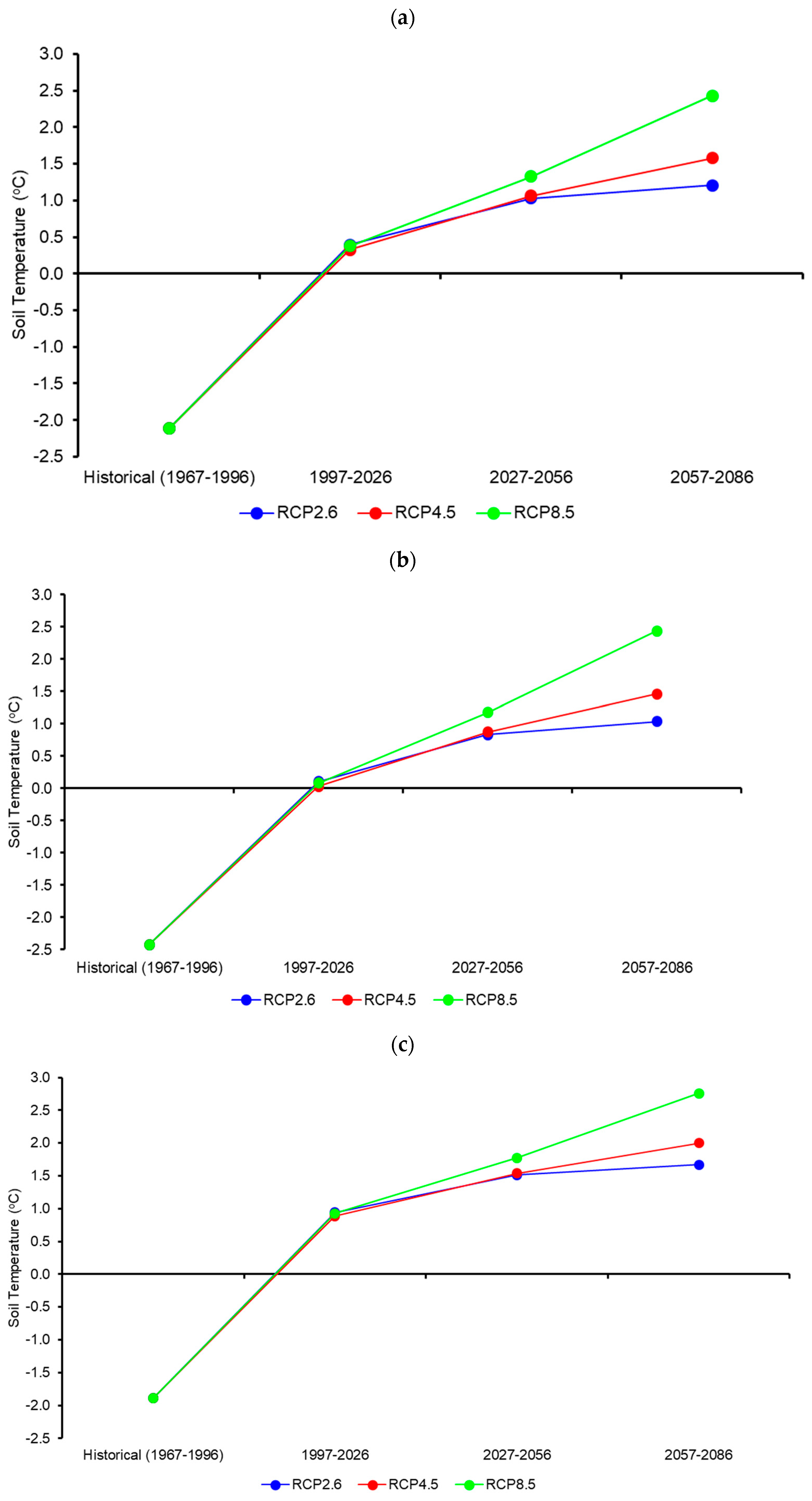
3.3.1. Annual
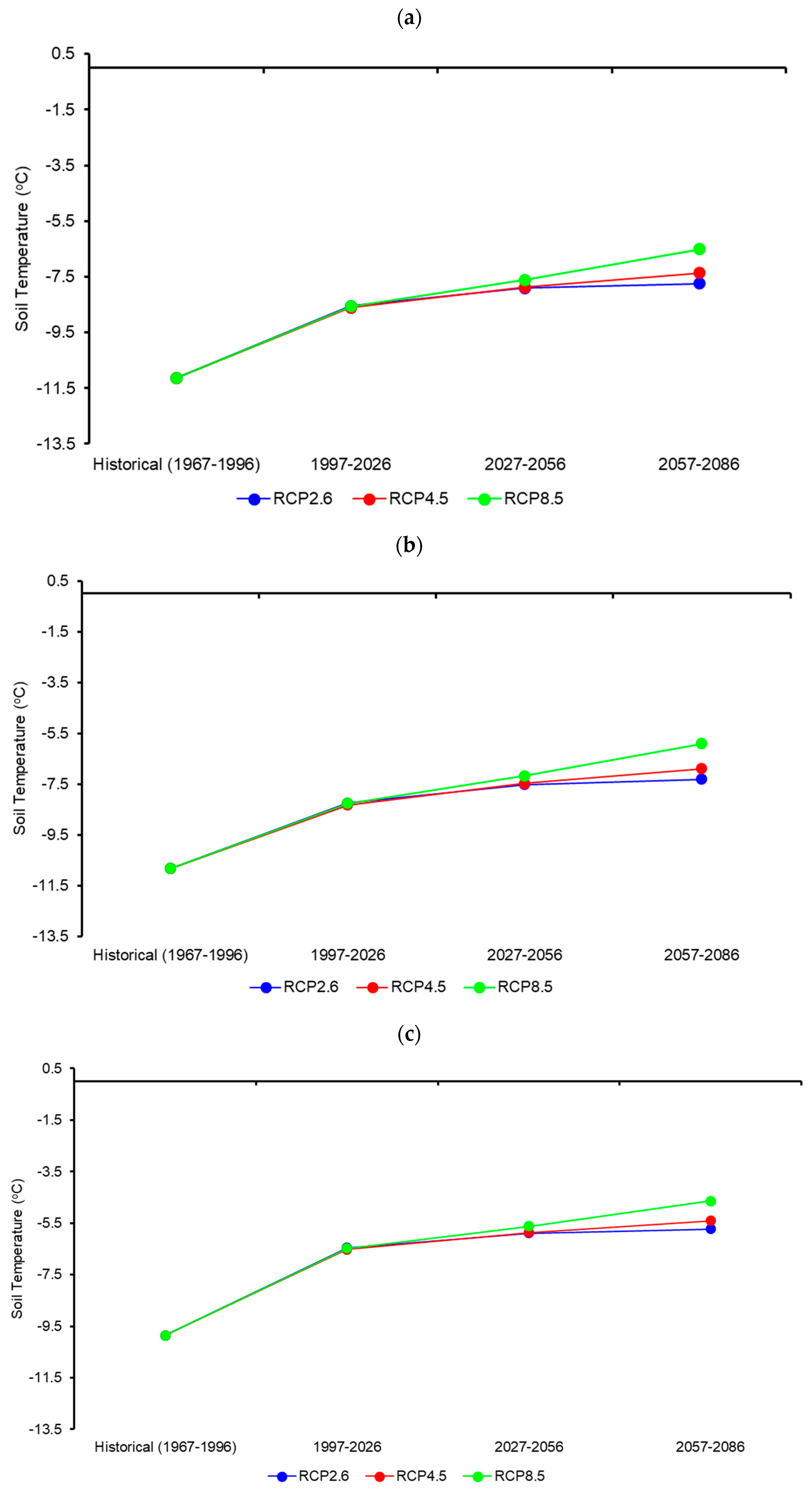
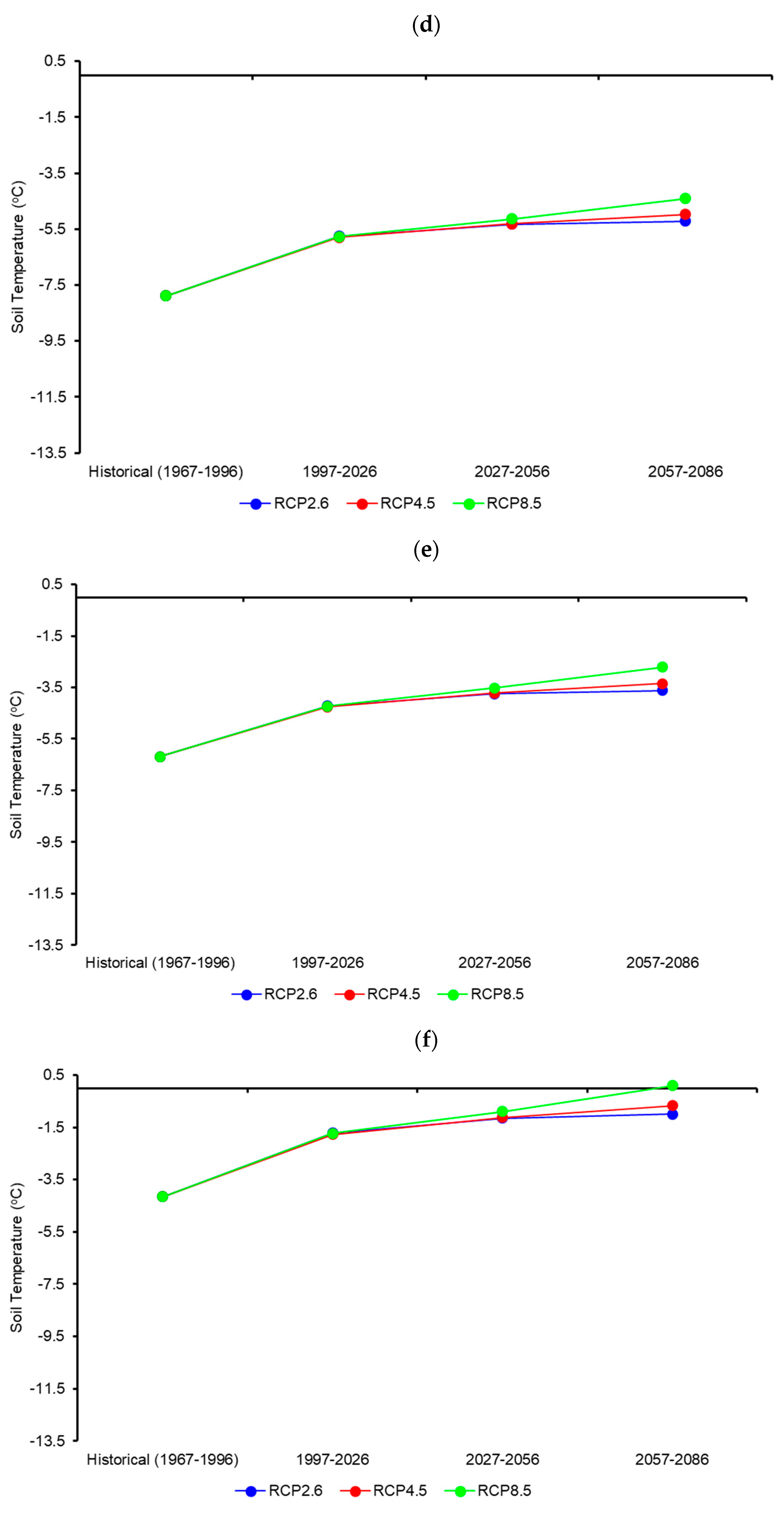
3.3.2. Winter
4. Discussion
4.1. Historical Trends and Model Fitting
4.2. Projections
4.3. Uncertainties
4.3.1. Observation Uncertainties
4.3.2. Modelling and Projections Uncertainties
4.4. Implications
4.4.1. Implications to the Environment
4.4.2. Implications to Airports
4.5. Long-Term Monitoring Network
5. Conclusions
Author Contributions
Funding
Institutional Review Board Statement
Informed Consent Statement
Data Availability Statement
Acknowledgments
Conflicts of Interest
References
- Graversen, R.G.; Mauritsen, T.; Tjernström, M.; Källén, E.; Svensson, G. Vertical structure of recent Arctic warming. Nature 2008, 451, 53–56. [Google Scholar] [CrossRef]
- Qian, B.; Gregorich, E.G.; Gameda, S.; Hopkins, D.W.; Wang, X.L. Observed soil temperature trends associated with climate change in Canada. J. Geophys. Res. Atmos. 2011, 116, D02106. [Google Scholar] [CrossRef]
- Stewart, E.; Tivy, A.; Howell, S.; Dawson, J.; Draper, D. Cruise Tourism and Sea Ice in Canada’s Hudson Bay Region. Arctic 2010, 63, 57–66. [Google Scholar] [CrossRef] [Green Version]
- Department of Energy, Mines and Resources Canada. The National Atlas of Canada, 5th ed.; Department of Energy, Mines and Resources Canada: Ottawa, ON, Canada, 1985. [Google Scholar] [CrossRef]
- Boucher, M.; Guimond, A. Assessing the Vulnerability of Ministère des Transports du Québec Infrastructure in Nunavik in a Context of Thawing Permafrost and the Development of an Adaptation Strategy. Cold Regions Engineering, Quebec City, QC, Canada, 19–22 August 2012; Doré, G., Morse, B., Eds.; American Society of Civil Engineers: Reston, VA, USA, 2012. [Google Scholar] [CrossRef]
- Oelke, C.; Zhang, T. A model study of circum-Arctic soil temperatures. Permafr. Periglac. Process. 2004, 15, 103–121. [Google Scholar] [CrossRef]
- Anderson, V.; Leung, A.C.W.; Mehdipoor, H.; Jänicke, B.; Milošević, D.; Oliveira, A.; Manavvi, S.; Kabano, P.; Dzyuban, Y.; Aguilar, R.; et al. Technological opportunities for sensing of the health effects of weather and climate change: A state-of-the-art-review. Int. J. Biometeorol. 2021, 65, 779–803. [Google Scholar] [CrossRef] [PubMed]
- Kelsey, K.C.; Pedersen, S.H.; Leffler, A.J.; Sexton, J.O.; Feng, M.; Welker, J.M. Winter snow and spring temperature have differential effects on vegetation phenology and productivity across Arctic plant communities. Glob. Chang. Biol. 2020, 27, 1572–1586. [Google Scholar] [CrossRef]
- Leung, A.; Gough, W. Air mass distribution and the heterogeneity of the climate change signal in the Hudson Bay/Foxe Basin region, Canada. Theor. Appl. Clim. 2016, 125, 583–592. [Google Scholar] [CrossRef]
- Beltrami, H.; Gosselin, C.; Mareschal, J.C. Ground surface temperatures in Canada: Spatial and temporal variability. Geophys. Res. Lett. 2003, 30, 1499. [Google Scholar] [CrossRef] [Green Version]
- Beltrami, H.; Bourlon, E.; Kellman, L.; González-Rouco, J.F. Spatial patterns of ground heat gain in the Northern Hemisphere. Geophys. Res. Lett. 2006, 33, L06717. [Google Scholar] [CrossRef] [Green Version]
- Tam, A.; Gough, W.A.; Xie, C. An Assessment of Potential Permafrost along a North-South Transect in Canada under Projected Climate Warming Scenarios from 2011 to 2100. Int. J. Clim. Chang. Impacts Responses 2015, 6, 1–18. [Google Scholar] [CrossRef]
- Xie, C.W.; Gough, W.A. Comments on thaw-freeze algorithms for multilayered soil, using the Stefan equation. Sci. Cold Arid Reg. 2017, 9, 525–533. [Google Scholar] [CrossRef]
- Jiang, Y.; Zhuang, Q.; Sitch, S.; O’Donnell, J.; Kicklighter, D.; Sokolov, A.; Melillo, J. Importance of soil thermal regime in terrestrial ecosystem carbon dynamics in the circumpolar north. Glob. Planet. Chang. 2016, 142, 28–40. [Google Scholar] [CrossRef] [Green Version]
- Harris, C.; Arenson, L.; Christiansen, H.H.; Etzelmüller, B.; Frauenfelder, R.; Gruber, S.; Haeberli, W.; Hauck, C.; Hölzle, M.; Humlum, O.; et al. Permafrost and climate in Europe: Monitoring and modelling thermal, geomorphological and geotechnical responses. Earth-Sci. Rev. 2009, 92, 117–171. [Google Scholar] [CrossRef] [Green Version]
- Gough, W.A.; Leung, A. Nature and fate of Hudson Bay permafrost. Reg. Environ. Chang. 2002, 2, 177–184. [Google Scholar] [CrossRef]
- Beltrami, H.; Kellman, L. An examination of short- and long-term air–ground temperature coupling. Glob. Planet. Chang. 2003, 38, 291–303. [Google Scholar] [CrossRef]
- Houle, D.; Bouffard, A.; Duchesne, L.; Logan, T.; Harvey, R. Projections of Future Soil Temperature and Water Content for Three Southern Quebec Forested Sites. J. Clim. 2012, 25, 7690–7701. [Google Scholar] [CrossRef]
- Fort Chimo Station Inspection Report; Environment Canada: Ottawa, ON, Canada, 1966.
- Fort Chimo Station Inspection Report; Environment Canada: Ottawa, ON, Canada, 1972.
- Kroeger, A. Changing Course: The Federal Government’s Program Review of 1994-95. In Hard Choices or No Choices: Assessing Program Review; Armit, A., Bourgault, J., Eds.; The Institute of Public Administration of Canada and Canadian Plains Research Center: Toronto, ON, Canada, 1996; pp. 21–28. [Google Scholar]
- Devine, K.; Environment and Climate Change Canada, Toronto, ON, Canada. Personal communication, 22 September 2017.
- Environment Canada. Canadian Climate Normals. Volume 9: Soil Temperature, Lake Evaporation, Days with Blowing Snow, Hail, Fog, Smoke/Haze, Frost; 1951–1980; Environment Canada: Downsview, ON, Canada, 1984. [Google Scholar]
- Mann, H.B. Nonparametric tests against trend. J. Econom. Soc. 1945, 13, 245–259. [Google Scholar] [CrossRef]
- Kendall, M.G. Rank Correlation Methods; Griffin: London, UK, 1975. [Google Scholar]
- Theil, H. A Rank-Invariant Method of Linear and Polynomial Regression Analysis. In Henri Theil’s Contributions to Economics and Econometrics; Springer: Dordrecht, The Netherlands, 1950. [Google Scholar] [CrossRef]
- Sen, P.K. Estimates of the regression coefficient based on Kendall’s Tau. J. Am. Stat. Assoc. 1968, 63, 1379–1389. [Google Scholar] [CrossRef]
- Hamed, K.H.; Rao, A.R. A modified Mann-Kendall trend test for autocorrelated data. J. Hydrol. 1998, 204, 182–196. [Google Scholar] [CrossRef]
- Pearson, K. Notes on regression and inheritance in the case of two parents. Proc. R. Soc. Lond. 1895, 58, 240–242. [Google Scholar]
- Wilby, R.; Dawson, C.; Barrow, E. SDSM—a decision support tool for the assessment of regional climate change impacts. Environ. Model. Softw. 2002, 17, 145–157. [Google Scholar] [CrossRef]
- Kalnay, E.; Kanamitsu, M.; Kistler, R.; Collins, W.; Deaven, D.; Gandin, L.; Iredell, M.; Saha, S.; White, G.; Woollen, J.; et al. The NCEP/NCAR 40-year reanalysis project. Bull. Am. Meteorol. Soc. 1996, 77, 437–471. [Google Scholar] [CrossRef] [Green Version]
- Stow, C.A.; Roessler, C.; Borsuk, M.E.; Bowen, J.D.; Reckhow, K.H. Comparison of Estuarine Water Quality Models for Total Maximum Daily Load Development in Neuse River Estuary. J. Water Resour. Plan. Manag. 2003, 129, 307–314. [Google Scholar] [CrossRef] [Green Version]
- Chylek, P.; Li, J.; Dubey, M.K.; Wang, M.; Lesins, G. Observed and model simulated 20th century Arctic temperature variability: Canadian Earth System Model CanESM2. Atmos. Chem. Phys. Discuss. 2011, 11, 22893–22907. [Google Scholar] [CrossRef]
- Verseghy, D.L. The Canadian land surface scheme (CLASS): Its history and future. Atmosphere-Ocean 2000, 38, 1–13. [Google Scholar] [CrossRef]
- Environment and Climate Change Canada. Canadian Centre for Climate Modelling and Analysis: CanESM2/CGCM4 model output. Available online: https://climate-modelling.canada.ca/climatemodeldata/cgcm4/CanESM2/rcp45/day/atmos/index.shtml (accessed on 27 September 2021).
- Braun, M.; Thiombiano, A.N.; Vieira, M.J.F.; Stadnyk, T.A. Representing climate evolution in ensembles of GCM simulations for the Hudson Bay System. Elem Sci Anth 2021, 9, 00011. [Google Scholar] [CrossRef]
- Swart, N.C.; Cole, J.N.S.; Kharin, V.V.; Lazare, M.; Scinocca, J.F.; Gillett, N.P.; Anstey, J.; Arora, V.; Christian, J.R.; Hanna, S.; et al. The Canadian Earth System Model version 5 (CanESM5.0.3). Geosci. Model Dev. 2019, 12, 4823–4873. [Google Scholar] [CrossRef] [Green Version]
- Climate Lab at the University of Toronto Localizer. University of Toronto Scarborough. Available online: http://climatechange.utsc.utoronto.ca (accessed on 15 April 2018).
- Meinshausen, M.; Smith, S.J.; Calvin, K.; Daniel, J.S.; Kainuma, M.L.T.; Lamarque, J.F.; Matsumoto, K.; Montzka, S.A.; Raper, S.C.B.; Riahi, K.; et al. The RCP greenhouse gas concentrations and their extensions from 1765 to 2300. Clim. Change 2011, 109, 213–241. [Google Scholar] [CrossRef] [Green Version]
- Environment Canada. Canadian Climate Normals 1961–1990. Available online: https://climate.weather.gc.ca/climate_normals/index_e.html#1961 (accessed on 16 September 2021).
- Environment Canada. Canadian Climate Normals 1971–2000. Available online: https://climate.weather.gc.ca/climate_normals/index_e.html#1971 (accessed on 16 September 2021).
- Environment Canada. Canadian Climate Normals 1981–2010. Available online: https://climate.weather.gc.ca/climate_normals/index_e.html#1981 (accessed on 16 September 2021).
- Jean, M. Évolution de la température du sol à Kuujjuaq, Quebec 1967–1989. Le Clim. 1991, 9, 39–48. [Google Scholar]
- Bourdeau-Goulet, S.; Hassanzadeh, E. Comparisons Between CMIP5 and CMIP6 Models: Simulations of Climate Indices Influencing Food Security, Infrastructure Resilience, and Human Health in Canada. Earth’s Futur. 2021, 9, e2021EF001995. [Google Scholar] [CrossRef]
- Skinner, W.R.; Flannigan, M.; Stocks, B.J.; Martell, D.L.; Wotton, B.M.; Todd, J.B.; Mason, J.A.; Logan, K.A.; Bosch, E.M. A 500 hPa synoptic wildland fire climatology for large Canadian forest fires, 1959–1996. Theor. Appl. Clim. 2002, 71, 157–169. [Google Scholar] [CrossRef]
- Phillips, C.L.; Torn, M.S.; Koven, C.D. Response of Soil Temperature to Climate Change in the CMIP5 Earth System Models. In Proceedings of the American Geophysical Union Fall Meeting 2014, San Francisco, CA, USA, 15–19 December 2014. Abstract Number B23K-0144. [Google Scholar]
- Zhang, Y.; Chen, W.; Smith, S.L.; Riseborough, D.W.; Cihlar, J. Soil temperature in Canada during the twentieth century: Complex responses to atmospheric climate change. J. Geophys. Res. Atmos. 2005, 110, D03112. [Google Scholar] [CrossRef]
- Nelson, F.E. (Un)frozen in Time. Science 2003, 299, 1673–1675. [Google Scholar] [CrossRef] [PubMed]
- Mühll, D.V.; Stucki, T.; Haeberli, W. In Borehole temperatures in alpine permafrost: A ten year series. In Proceedings of the Permafrost, Seventh International Conference, Yellowknife, NT, Canada, 23–27 June 1998; Lewkowicz, A., Allard, M., Eds.; Université Laval, Centre d’études nordiques, Collection Nordicana: Quebec City, QC, Canada; pp. 1089–1095. [Google Scholar]
- Zajch, A.; Gough, W.A. Seasonal sensitivity to atmospheric and ground surface temperature changes of an open earth-air heat exchanger in Canadian climates. Geothermics 2020, 89, 101914. [Google Scholar] [CrossRef]
- Gómez, I.; Caselles, V.; Estrela, M.J.; Niclòs, R. Impact of Initial Soil Temperature Derived from Remote Sensing and Numerical Weather Prediction Datasets on the Simulation of Extreme Heat Events. Remote. Sens. 2016, 8, 589. [Google Scholar] [CrossRef] [Green Version]
- Zhang, Y.; Sherstiukov, A.B.; Qian, B.; Kokelj, S.V.; Lantz, T.C. Impacts of snow on soil temperature observed across the circumpolar north. Environ. Res. Lett. 2018, 13, 044012. [Google Scholar] [CrossRef] [Green Version]
- Fort Chimo Station Inspection Report; Environment Canada: Ottawa, ON, Canada, 1978.
- Majorowicz, M.; Minea, V. In Geological, Economical and Environmental Assessment of Combined Geothermal Power and Heat Generation in Québec, Canada. In Proceedings of the World Geothermal Congress 2015, Melbourne, VIC, Australia, 19–25 April 2015. [Google Scholar]
- Miralles, D.G.; Berg, M.J.V.D.; Teuling, A.; De Jeu, R.A.M. Soil moisture-temperature coupling: A multiscale observational analysis. Geophys. Res. Lett. 2012, 39, L21707. [Google Scholar] [CrossRef] [Green Version]
- Yin, G.-A.; Niu, F.-J.; Lin, Z.-J.; Luo, J.; Liu, M.-H. Data-driven spatiotemporal projections of shallow permafrost based on CMIP6 across the Qinghai–Tibet Plateau at 1 km2 scale. Adv. Clim. Chang. Res. 2021, 12, 814–827. [Google Scholar] [CrossRef]
- Slater, A.; Lawrence, D. Diagnosing Present and Future Permafrost from Climate Models. J. Clim. 2013, 26, 5608–5623. [Google Scholar] [CrossRef] [Green Version]
- Slater, A.G.; Schlosser, C.A.; Desborough, C.E.; Pitman, A.; Henderson-Sellers, A.; Robock, A.; Vinnikov, K.Y.; Entin, J.; Mitchell, K.; Chen, F.; et al. The Representation of Snow in Land Surface Schemes: Results from PILPS 2(d). J. Hydrometeorol. 2001, 2, 7–25. [Google Scholar] [CrossRef] [Green Version]
- Koven, C.D.; Riley, W.J.; Stern, A. Analysis of Permafrost Thermal Dynamics and Response to Climate Change in the CMIP5 Earth System Models. J. Clim. 2013, 26, 1877–1900. [Google Scholar] [CrossRef] [Green Version]
- Burke, E.J.; Zhang, Y.; Krinner, G. Evaluating permafrost physics in the Coupled Model Intercomparison Project 6 (CMIP6) models and their sensitivity to climate change. Cryosphere 2020, 14, 3155–3174. [Google Scholar] [CrossRef]
- Yokohata, T.; Saito, K.; Takata, K.; Nitta, T.; Satoh, Y.; Hajima, T.; Sueyoshi, T.; Iwahana, G. Model improvement and future projection of permafrost processes in a global land surface model. Prog. Earth Planet. Sci. 2020, 7, 69. [Google Scholar] [CrossRef]
- Melton, J.R.; Arora, V.K.; Wisernig-Cojoc, E.; Seiler, C.; Fortier, M.; Chan, E.; Teckentrup, L. CLASSIC v1.0: The open-source community successor to the Canadian Land Surface Scheme (CLASS) and the Canadian Terrestrial Ecosystem Model (CTEM)—Part 1: Model framework and site-level performance. Geosci. Model Dev. 2020, 13, 2825–2850. [Google Scholar] [CrossRef]
- Wang, B.; Allard, M. Recent climatic trend and thermal response of permafrost in Salluit, Northern Quebec, Canada. Permafr. Periglac. Process. 1995, 6, 221–233. [Google Scholar] [CrossRef]
- Allard, M.; Wang, B.; Pilon, J.A. Recent Cooling along the Southern Shore of Hudson Strait, Quebec, Canada, Documented from Permafrost Temperature Measurements. Arct. Alp. Res. 1995, 27, 157–166. [Google Scholar] [CrossRef]
- Doré, G.; Ficheur, A.; Guimond, A.; Boucher, M. Performance and Cost-Effectiveness of Thermal Stabilization Techniques Used at the Tasiujaq Airstrip. In Cold Regions Engineering, 19–22 August 2012, Quebec City, QC, Canada; Doré, G., Morse, B., Eds.; American Society of Civil Engineers: Reston, VA, USA, 2012. [Google Scholar] [CrossRef]
- Fortier, R.; Leblanc, A.-M.; Yu, W. Impacts of permafrost degradation on a road embankment at Umiujaq in Nunavik (Quebec), Canada. Can. Geotech. J. 2011, 48, 720–740. [Google Scholar] [CrossRef]
- Burke, E.J.; Chadburn, S.; Huntingford, C.; Jones, C.D. CO2 loss by permafrost thawing implies additional emissions reductions to limit warming to 1.5 or 2 °C. Environ. Res. Lett. 2018, 13, 024024. [Google Scholar] [CrossRef]
- Todd-Brown, K.E.O.; Randerson, J.T.; Hopkins, F.; Arora, V.; Hajima, T.; Jones, C.; Shevliakova, E.; Tjiputra, J.; Volodin, E.; Wu, T.; et al. Changes in soil organic carbon storage predicted by Earth system models during the 21st century. Biogeosciences 2014, 11, 2341–2356. [Google Scholar] [CrossRef] [Green Version]
- Drijfhout, S.; Bathiany, S.; Beaulieu, C.; Brovkin, V.; Claussen, M.; Huntingford, C.; Scheffer, M.; Sgubin, G.; Swingedouw, D. Catalogue of abrupt shifts in Intergovernmental Panel on Climate Change climate models. Proc. Natl. Acad. Sci. USA 2015, 112, E5777–E5786. [Google Scholar] [CrossRef] [Green Version]
- Yang, Z.; Fang, W.; Lu, X.; Sheng, G.-P.; Graham, D.; Liang, L.; Wullschleger, S.D.; Gu, B. Warming increases methylmercury production in an Arctic soil. Environ. Pollut. 2016, 214, 504–509. [Google Scholar] [CrossRef] [PubMed]
- Oldenborger, G.A.; LeBlanc, A.-M. Geophysical characterization of permafrost terrain at Iqaluit International Airport, Nunavut. J. Appl. Geophys. 2015, 123, 36–49. [Google Scholar] [CrossRef]
- Leung, A.C.W.; Gough, W.A.; Shi, Y. Identifying Frostquakes in Central Canada and Neighbouring Regions in the United States with Social Media. In Citizen Empowered Mapping; Leitner, M., Jokar Arsanjani, J., Eds.; Springer Nature: Cham, Switzerland, 2017; pp. 201–222. [Google Scholar]
- Ghias, M.S.; Therrien, R.; Molson, J.; Lemieux, J.-M. Controls on permafrost thaw in a coupled groundwater-flow and heat-transport system: Iqaluit Airport, Nunavut, Canada. Hydrogeol. J. 2016, 25, 657–673. [Google Scholar] [CrossRef]
- Kloepfer, C. An airport public–private partnership in the Canadian Arctic. J. Airport Manage. 2017, 11, 136–146. [Google Scholar]
- Nelson, F.E.; Anisimov, O.A.; Shiklomanov, N.I. Climate Change and Hazard Zonation in the Circum-Arctic Permafrost Regions. Nat. Hazards 2002, 26, 203–225. [Google Scholar] [CrossRef]
- Leung, A.C.W.; Gough, W.A.; Butler, K.A.; Mohsin, T.; Hewer, M.J. Characterizing observed surface wind speed in the Hudson Bay and Labrador regions of Canada from an aviation perspective. Int. J. Biometeorol. 2020, 1–15. [Google Scholar] [CrossRef] [PubMed]
- Kim, A.M.; Li, H. Incorporating the impacts of climate change in transportation infrastructure decision models. Transp. Res. Part A Policy Pract. 2020, 134, 271–287. [Google Scholar] [CrossRef]
- Johnston, G.H. Design and Performance of the Inuvik, N.W.T., Airstrip. In Proceedings of the Fourth Canadian Permafrost Conference, Calgary, AB, Canada, 2–6 March 1981; National Research Council of Canada: Ottawa, Canada, 1982; pp. 577–585. Available online: https://nrc-publications.canada.ca/eng/view/object/?id=ef120dbb-f6b6-4eb9-a28c-cb994e5a29db (accessed on 4 January 2022).
- Judge, A.; Tucker, C.; Pilon, J.; Moorman, B. Remote Sensing of Permafrost by Ground-Penetrating Radar at Two Airports in Arctic Canada. Arctic 1991, 44 (Supp. 1), 40–48. [Google Scholar] [CrossRef]
- Allen, M.J.; Vanos, J.; Hondula, D.M.; Vecellio, D.J.; Knight, D.; Mehdipoor, H.; Lucas, R.; Fuhrmann, C.; Lokys, H.; Lees, A.; et al. Supporting sustainability initiatives through biometeorology education and training. Int. J. Biometeorol. 2017, 61, 93–106. [Google Scholar] [CrossRef]
- Bender, G.; Sperry, R. Airport buildings: A key opportunity for sustainability in aviation. J. Airport Manage. 2020, 14, 234–245. [Google Scholar]
- Leung, A.C.W.; Gough, W.A.; Butler, K.A. Changes in Fog, Ice Fog, and Low Visibility in the Hudson Bay Region: Impacts on Aviation. Atmosphere 2020, 11, 186. [Google Scholar] [CrossRef] [Green Version]
- Meyer, S.J.; Hubbard, K.G. Nonfederal Automated Weather Stations and Networks in the United States in the United States and Canada: A Preliminary Survey. Bull. Am. Meteorol. Soc. 1992, 73, 449–457. [Google Scholar] [CrossRef] [Green Version]


| Soil Depth | Mean (°C) | Trend (°C/Decade) | ||
|---|---|---|---|---|
| Annual | Winter | Annual | Winter | |
| 5 cm | −2.1 | −11.1 | +1.2 * | +1.9 * |
| 10 cm | −2.4 | −10.8 | +1.1 * | +1.7 ^ |
| 20 cm | −1.9 | −9.9 | +1.3 ** | +1.4 ^ |
| 50 cm | −1.4 | −7.9 | +1.0 * | +1.2 |
| 100 cm | −1.6 | −6.2 | +0.9 ^ | +0.8 |
| 150 cm | −1.9 | −4.2 | +1.1 ** | +1.0 |
| Soil Depth | r Coefficient (Daily) | r Coefficient (Monthly Average) | ||
|---|---|---|---|---|
| Annual | Winter | Annual | Winter | |
| 5 cm | 0.845 | 0.453 | 0.955 | 0.746 |
| 10 cm | 0.847 | 0.452 | 0.951 | 0.733 |
| 20 cm | 0.848 | 0.450 | 0.946 | 0.722 |
| 50 cm | 0.819 | 0.391 | 0.906 | 0.597 |
| 100 cm | 0.721 | 0.268 | 0.797 | 0.407 |
| 150 cm | 0.455 | 0.087 | 0.514 | 0.147 |
| Soil Depth | r Correlation | |||||||
|---|---|---|---|---|---|---|---|---|
| Surface Specific Humidity | Mean 2 m Air Temperature | 500 hPa Geopotential Height | Specific Humidity at 850 hPa | |||||
| NCEP | CanESM2 | NCEP | CanESM2 | NCEP | CanESM2 | NCEP | CanESM2 | |
| 5 cm | 0.825 | 0.828 | 0.825 | 0.821 | 0.696 | 0.756 | 0.700 | 0.699 |
| 10 cm | 0.826 | 0.832 | 0.828 | 0.830 | 0.693 | 0.752 | 0.700 | 0.697 |
| 20 cm | 0.812 | 0.824 | 0.806 | 0.825 | 0.673 | 0.732 | 0.689 | 0.687 |
| 50 cm | 0.817 | 0.833 | 0.811 | 0.831 | 0.658 | 0.711 | 0.694 | 0.682 |
| 100 cm | 0.728 | 0.758 | 0.722 | 0.763 | 0.557 | 0.601 | 0.618 | 0.599 |
| 150 cm | 0.466 | 0.504 | 0.462 | 0.525 | 0.314 | 0.337 | 0.390 | 0.365 |
| Modelled Depth | MEF Value (−1 to +1) | RMSE | MAE |
|---|---|---|---|
| 5 cm | 0.83 | 4.590301 | 3.471129 |
| 10 cm | 0.83 | 4.185074 | 3.088709 |
| 20 cm | 0.84 | 3.778079 | 2.731346 |
| 50 cm | 0.85 | 3.160122 | 2.140639 |
| 100 cm | 0.81 | 2.825081 | 1.797228 |
| 150 cm | 0.66 | 2.702048 | 1.673864 |
Publisher’s Note: MDPI stays neutral with regard to jurisdictional claims in published maps and institutional affiliations. |
© 2022 by the authors. Licensee MDPI, Basel, Switzerland. This article is an open access article distributed under the terms and conditions of the Creative Commons Attribution (CC BY) license (https://creativecommons.org/licenses/by/4.0/).
Share and Cite
Leung, A.C.W.; Gough, W.A.; Mohsin, T. Analysing Historical and Modelling Future Soil Temperature at Kuujjuaq, Quebec (Canada): Implications on Aviation Infrastructure. Forecasting 2022, 4, 95-125. https://0-doi-org.brum.beds.ac.uk/10.3390/forecast4010006
Leung ACW, Gough WA, Mohsin T. Analysing Historical and Modelling Future Soil Temperature at Kuujjuaq, Quebec (Canada): Implications on Aviation Infrastructure. Forecasting. 2022; 4(1):95-125. https://0-doi-org.brum.beds.ac.uk/10.3390/forecast4010006
Chicago/Turabian StyleLeung, Andrew C. W., William A. Gough, and Tanzina Mohsin. 2022. "Analysing Historical and Modelling Future Soil Temperature at Kuujjuaq, Quebec (Canada): Implications on Aviation Infrastructure" Forecasting 4, no. 1: 95-125. https://0-doi-org.brum.beds.ac.uk/10.3390/forecast4010006