Trend Lines and Japanese Candlesticks Applied to the Forecasting of Wind Speed Data Series

Abstract

One of the most critical issues for wind energy exploitation is the high variability of the resource, resulting in very difficult forecasting of the power that wind farms can grant. A vast literature has therefore been devoted to wind speed and wind power quantitative forecasting, using different techniques. The widely used statistical and learning models that are based on a continuation in the future of the series’ past behaviour offer a performance that may be much less satisfactory when the values suddenly change their trend. The application to wind speed data of two techniques usually employed for the technical analysis of financial series–namely support and resistances identification and candlestick charts–is investigated here, with the main aim to detect inversion points in the series. They are applied to wind speed data series for two locations in Spain and Italy. The proposed indicators confirm their usefulness in identifying peculiar behaviours in the system and conditions where the trend may be expected to change. This additional information offered to the forecasting algorithms may also be included in innovative approaches, e.g., based on machine learning.

1. Introduction

Wind energy is one of the fastest-growing renewable energies. This is not surprising, given its very large potential [1], with the additional advantage that it is distributed all over the world even with obvious differences between regions. Moreover, its exploitation can rely on technologically mature solutions. Nonetheless, open issues remain, both technical and environmental or socio-political. Among the first, one of the most critical aspects is the high variability of wind speed, which makes the prediction of energy output very difficult. As a consequence, a very large number of studies have been devoted to models, techniques and algorithms to forecast wind speed and consequently power output from single turbines or wind farms. Actually, power prediction is further complicated by the fact that in real cases its relation with wind speed is in general more complex than in theory (power related to the cube of wind speed by means of air density, rotor swept area and coefficient of performance); the power curve of the aerogenerator may vary with turbine ageing or weather conditions (e.g., in presence of icing) and the mutual disturbances between wind turbines in a wind farm may depend on the wind direction in addition to the speed itself [2,3]. Despite their importance, these aspects are out of the scope of this paper, which will be focused on wind speed alone.

Forecasting tools range from physical models (nowadays also including Computational Fluid Dynamics up to the mesoscale) to statistical approaches and artificial intelligence techniques. An introduction to the most used methods can be found in the book edited by Kariniotakis [4] and in the paper by Chang [5], while reviews about the topic can be found in the works of Koračin et al. [1], Foley et al. [6], Barbosa de Alencar et al. [7], Lawan et al. [8] and Lei et al. [9]. Further references about the different types of predictive models can be found in the papers by Jursa and Rohrig [10], Wang et al. [11] and Soman and Zareipour [12]. The latter work in particular includes interesting summarizing tables on different time scales and corresponding applications. More peculiar techniques, e.g., linked to deterministic chaos or “borrowed” from other fields including finance, are also described in the literature [13,14]. In the last years, a major focus has been on the application of learning algorithms and hybrid models [15,16,17,18,19]. Further references devoted to the last class of techniques can be found in [19]. Wavelets and decomposition models were also tested [20,21].

Despite the different strategies, all the techniques that are based on a continuation in the future of the past trends fail or at least have major difficulties when the values suddenly change their direction. Prediction of these points of inversion would be consequently very useful to correct the model forecasts or at least to “issue an alert” about their reliability. In addition, such information might also be included in innovative forecasting approaches, e.g., based on machine learning techniques.

With this aim, two tools usually employed for the analysis of financial series were tested in this work: support and resistance lines and candlestick charts.

They were applied to wind speed data series acquired by two meteorological stations, located at Capo Mele (in the province of Savona, Liguria, Italy) and Los Montes del Cierzo (near Tudela, Navarra, Spain).

The innovative contribution of the work is to assess if these techniques, originally developed to study other topics, may offer useful insight also in the analysis of wind series, namely in identifying “points”—i.e., time instants—at which changes in the data behaviour are likely to occur. At present, the work is limited to the analysis of the potentialities of the two techniques to identify continuation and inversion points in the series. The combination of the techniques with forecasting algorithms, either conventional or based on artificial intelligence, will be among the “future work” for the development of this approach.

2. Technical Analysis

“Technical analysis” is a group of techniques typically aimed at forecasting the values of financial data series by means of tools that focus purely on the past behaviour of the data (mainly prices and volumes) [22]. It does not try to assess the intrinsic value of the stocks by means of information about the issuing company or the micro- and macroeconomic scenario, as it is on the contrary done in the so-called “fundamental analysis”. The underlying assumption is that past data can provide significant information to predict future behaviour, both short- and middle- or long-term. As technical analysis works with pure numbers, with no attribution of specific meaning, the rationale underlying this work is that its techniques may be applied also to time series in other fields. The aim is to verify if such techniques–even if not able to provide a quantitative forecast–can offer useful information on series reversals. Among the many tools available for technical analysis, support and resistance lines and candlestick charts—which can be particularly suited for reversal and continuation detection—were selected for this work. Implementation of the two techniques in automated tools was not performed; trend lines and candlesticks were manually identified in the investigated series.

3. Support and Resistance Lines

The “support and resistance lines” technique is based on the concept of trend, that is the general direction in which the data series is headed [23,24]. For financial series, it is usually the price direction; for wind series, it is the direction in which the wind speed series is headed. For both cases, trends are in general difficult to identify because the time series are always far more complex than straight lines, with a series of highs and lows over time that are characterized by many different superposed frequencies. For wind speed, this behaviour is exactly what makes wind energy difficult to exploit.

Differently from linear regression in statistics, a trend line in technical analysis is traced by connecting lower lows or higher highs. An uptrend is present when such a line has a positive slope, while a downtrend is characterized by a negative slope. A sideways or horizontal trend presents peaks and troughs of the series with scarcely significant upward/downward movements. The data series arriving to cross the trend line may cut it or “bounce” on it. In the latter case, if the series arrives from above and rebounds towards higher values, the trend line is called a “support”; in the opposite case (approach from below and return to lower values), it is called a “resistance”. After a rebound, the time series may again invert its path and “test” the trend line again: the number of times in which a support or resistance level is able to resist crossing gives its strength.

In finance, supports are present when the demand is strong enough to avoid a further price decrease, while resistances appear when selling prevents prices from further rising; for wind speed, the support and resistance levels are summarizing indicators of the minimum or maximum values that the wind speed may reach in a certain region (e.g., due to its orography and the surrounding environment: sea, lakes, cities, trees, woods and forest, tree lines and rock formations that constitute obstacles able to appreciably decrease the wind speed and to create turbulence) and in a certain period (e.g., during a season or a day or an hour).

When a trend line is broken (i.e., crossed by the data series), new levels of support and resistance are generally established and the previous ones may reverse their role: a trend line that was a support may become a resistance, and vice versa.

Supports and resistances are typically used in finance to identify when a trend is about to reverse, so that proper trading decisions may be taken. For wind energy, breaking a trend line gives a signal that the data general direction is likely to change, so the predictions of forecasting models purely based on continuation may not be reliable.

4. Japanese Candlesticks Charts

The “candlesticks” technique appears to have been originally invented in Japan (either in the second half of the 18th century or in the 19th century according to different sources) for rice trade; then, in the 20th century, it gained widespread use for financial analysis [25,26]. In the latter use, a candlestick is a drawing that displays the highest, lowest, opening and closing values of the price (named high, low, open, close) within a selected time span. Its shape is that of a box plot, i.e., of a box with two whiskers: the box is called the “real body” and covers the span between open and close. It is typically coloured depending on if the closing price has been higher (“hollow” candlestick) or lower (“filled” candlestick) than the opening price, e.g., in their black and white versions (which will be used in this study) it is filled with white in the first case and with black in the second. The segments above and below the real body are usually called “shadows”: they extend to the extreme–minimum and maximum–prices of the session.

Translating the concept for the wind data series, the first, last, minimum, and maximum wind speed values within the observation window will be used to draw the candlestick body and the shadows.

Apart from their visual appeal, candlestick charts are often used because they are relatively easy to interpret. In white candlesticks, the close is higher than the open one, which indicates buying pressure in the trading analysis, increasing wind speed in the present analysis; black candlesticks, in which the open is higher than the close, indicate selling pressure in the trading analysis and decreasing wind speed in this analysis.

The length of the real body is another important indicator: a short body means little variations in the value due to consolidation in finance and a fairly constant speed for wind energy, whilst a long body evidences an intense buying or selling activity in finance, a significant variation over the observation period for wind speed. In finance, long hollow candlesticks are often “bullish” (the bull is the symbol of market rise) and long filled ones “bearish” (the bear is the symbol of market decline), but long candlesticks may also be a signal of an incoming turning point due to the encounter of support or resistance. For wind analysis, beyond the obvious meaning that in the observation period, the wind speed values covered a wide range, the second message is the one of major interest to forecast the turning points.

Concerning the shadows, short ones indicate that most of the trading or the wind speed oscillation was confined near the open and close; long ones on the contrary show that prices or wind speed extended well past the open and close, evidencing a higher fluctuation that may be an indicator of an “uncertain” behaviour and may imply a close change in trend.

In addition to the evaluation of single candlesticks, the identification of particular sequences of candlesticks–named “patterns”—are considered of primary importance in candlestick analysis. Many different patterns can be identified, and their detailed description is out of the scope of this work. The focus here will be only on some patterns that are more strongly related to changes in the data trends; they will be directly introduced in the Results section. In Appendix A, a reference table (

Table A1. Examples of some of the most used candlestick patterns for inversion, indecision and continuation, with their descriptions.

Candlestick Pattern	Description	Examples of Occurrence in the Los Montes del Cierzo Wind Speed Series
“Bullish” Patterns (Trend Inversion, with Values of the Data Series that Start to Rise, Is Expected)
	After a decreasing trend, a black candlestick is followed and “engulfed” by a longer white one that completely overlaps it.	Summer week, 2 m and 10 m, approaching August 3rd Summer week, 2 m and 10 m, between August 3rd and August 4th
	After a decreasing trend, a candlestick with a small real body, no upper shadow and a long lower shadow appears. The candlestick colour is of minor importance.	Winter week, 2 m, approaching January 5th Spring week, 2 m, between April 7th and April 8th
	After a decreasing trend, a candlestick with a small real body, no lower shadow and a long upper shadow appears. The candlestick colour is of minor importance.	Spring week, 2 m and 10 m, immediately after April 1st Spring week, 2 m and 10 m, between April 3rd and April 4th
	After a decreasing trend, a candlestick with a very small or no real body (in this case named doji) appears. The candlestick colour is of minor importance.	Summer Week, 10 m, immediately after Aug 1st Autumn Week, 2 m, approaching November 11th
	After a decreasing trend, a black candlestick, followed by a white one, appear, in which the second period opening is lower than the previous period closure; however, the values then rise significantly.	Summer week, 2 m, between August 4th and August 5th Summer week, 10 m, between August 7th and August 8th
	After a decreasing trend, a black candlestick, followed by a white one—having real bodies of similar height and both with short or no lower shadows—appear.	Summer week, 10 m, between August 3rd and August 4th Winter week, 2 m, between January 1st and January 2nd
“Bearish” Patterns (Trend Inversion, with Values of the Data Series that Start to Decrease, Is Expected)
	After a rising trend, a white candlestick, followed by a black one, appear, in which the second period opening is higher than the previous period closure; however, the values then decrease significantly.	Winter week, 10 m, between January 7th and January 8th Spring week, 10 m, approaching April 2nd
	After a rising trend, a white candlestick is followed and “engulfed” by a longer black one that completely overlaps it.	Summer week, 2 m and 10 m, approaching August 3rd Summer week, 2 m and 10 m, between August 3rd and August 4th
	After a rising trend, a candlestick with a very small or no real body (in this case named doji) appears. The candlestick color is of minor importance.	Summer week, 2 m, between August 1st and August 2nd Spring week, 10 m, between April 6th and April 7th
	After a rising trend, a candlestick with a small real body, no upper shadow and a long lower shadow appears. The candlestick colour is of minor importance.	Summer week, 10 m, between August 1st and August 2nd Autumn week, 10 m, approaching November 2nd
	After a rising trend, a candlestick with a small real body, no lower shadow and a long upper shadow appears. The candlestick colour is of minor importance.	Summer week, 2 m and 10 m, approaching August 4th Autumn week, 2 m and 10 m, between November 1st and November 2nd
	After a rising trend, a white candlestick, followed by a black one—having real bodies of similar height and both with short or no lower shadows—appear.	Autumn week, 2 m, between November 3rd and November 4th Winter week, 10 m, between January 4th and January 5th
“Indecision” Patterns (The Behaviour of the Series Depends on the Conditions)
Description		Examples of Occurrence in the Analysed Wind Data Series
After a trend, a long candlestick, followed by a small one, appear. The colours of the candles are usually different, but this is not mandatory. Depending on the general situation and on the relative positions of the candles, a change in trend towards an inversion or a “lateral” (nearly horizontal) evolution may occur.		Summer week, 10 m, approaching August 5th Winter week, 2 m, between January 5th and January 6th
Description		Examples of Occurrence in the Analysed Wind Data Series
A candlestick with very small or no real body (doji) and long shadows appears, but the trend is not reversed. The longer are the shadows, the most significant is the “indecision” of the data series.		Summer week, 2 m, approaching August 3rd Summer week, 2 m and 10 m, between August 3rd and August 4th
“Continuation” Patterns (The Series Will Not Change Trend)
	A five-candlesticks pattern in which three relatively short-bodied white candlesticks are bounded by two long black candlesticks. “Bullish” forces are not enough to change the decreasing trend.	Autumn week, 2 m, approaching November 2nd Spring week, 10 m, approaching April 6th
	A five-candlesticks pattern in which three relatively short-bodied black candlesticks are bounded by two long white candlesticks. “Bearish” forces are not enough to change the increasing trend.	Spring week, 2 m, after April 4th Spring week, 2 m, April 5th
	A sequence of three black candlesticks, with relatively long bodies. The decreasing trend is stronger if the opening of a period is lower than the closure of the previous one.	Winter week, 2 m, between January 2nd and January 3rd Spring week, 2 m and 10 m, approaching April 2nd
	A sequence of three white candlesticks, with relatively long bodies. The rising trend is stronger if the opening of a period is higher than the closure of the previous one.	Autumn week, 2 m and 10 m, between November 1st and November 2nd Winter week, 2 m and 10 m, between January 5th and January 6th

) is presented, including a selection of the most used candlesticks patterns, grouped according to their meaning for the financial market and corresponding meaning in the analysis of wind speed series. The dash–dot arrows represent the data trends (rising or decreasing) before and after the drawn candlesticks, completing each candlestick pattern. Further details can be found on specialized books and Web sites [25,26,27,28,29].

5. Results and Analysis

In the following, results of the application of the support and resistance lines and candlesticks charts to wind speed data series acquired at two locations will be described. Los Montes del Cierzo, near Tudela (Navarra, Spain, 314 m a.s.l.), and Capo Mele (in province of Savona, Liguria, Italy, 221 m a.s.l.) were selected. Los Montes del Cierzo data were acquired both at 2 m and 10 m above the ground and have a time resolution of 10 min; Capo Mele data have a time resolution of 1 h. Data from 2016 and 2017 were taken into consideration.

5.1. Support and Resistance Lines and Trending Channels

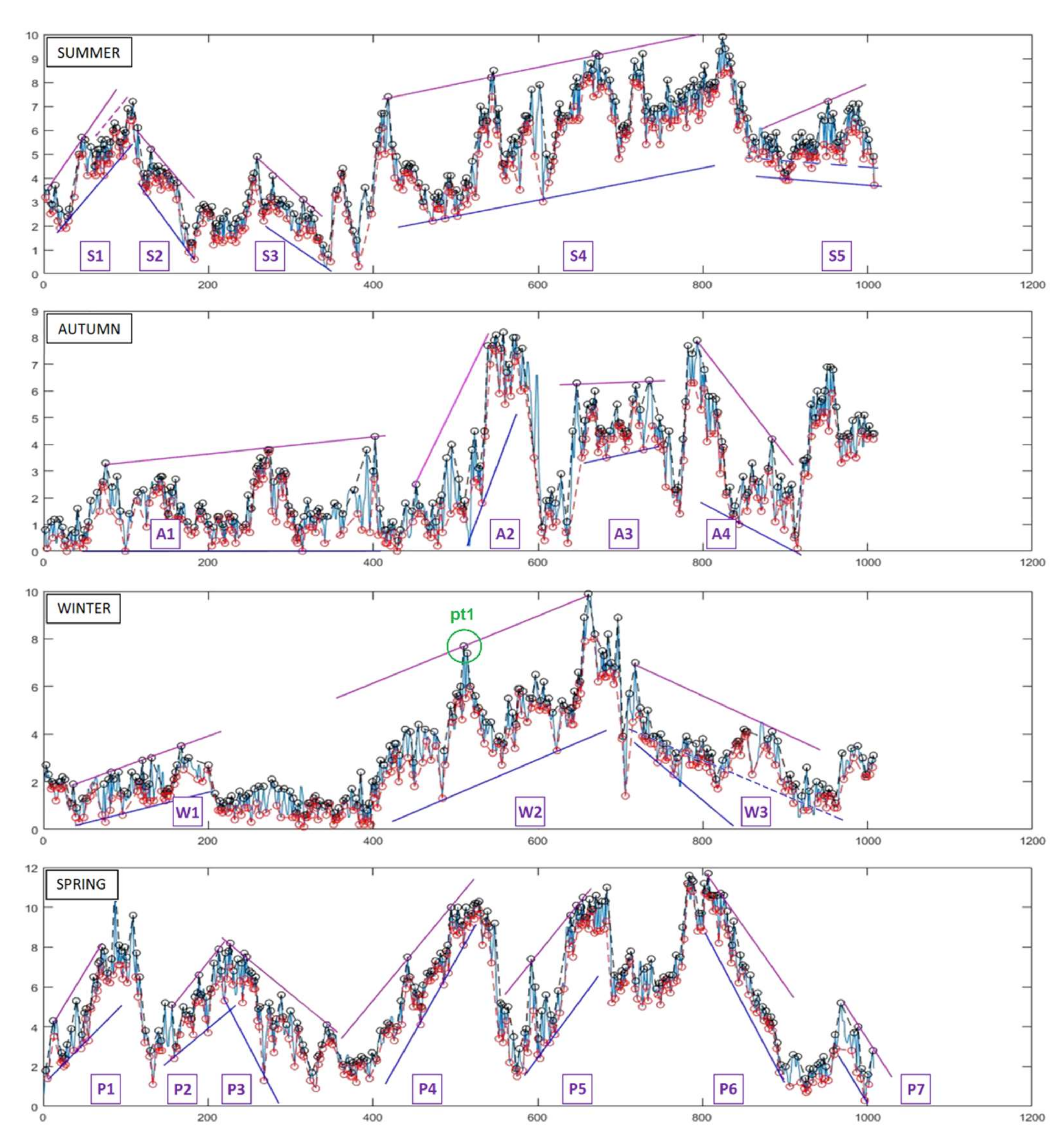
Figure 1 shows support and resistance lines identified in wind speed data series at the Los Montes del Cierzo location, 10 m above the ground, for four weeks selected from the whole year as representatives of the four seasons. The time resolution is 10 min, so each series includes 1008 values. Black and red circles are used to enhance the visualization of the local maxima and minima.

Starting from summer, in the first week of August 2016 five pairs of support/resistance lines can be identified. In the first one (S1), wind speed increases and the support and resistance lines diverge (the initial gap between them is smaller than the final one). The indication is therefore of a progressive increase with enlarging oscillations between minima and maxima. In finance, it would be a “bullish” trend with an increase in volatility. At a certain point, the values stop reaching the top resistance line and a second one (dashed in the chart) appears. The series “tests” this new line, but it is not able to cut it. The chart is therefore giving an alert for an incoming turning point that is soon confirmed: the wind speed starts decreasing.

The second pair of lines (S2) follows this decrease, which has a reducing gap between the beginning and the end. When the values bounce twice on the lower (support) line, the wind speed starts rising again. Completely analogous is the behaviour within the third pair (S3).

The fourth pair (S4) is probably the most interesting one for this week: its length proves that it is a strong trend, within which the wind speed increases with confined oscillations between the support and resistance lines (that are almost parallel). This trend ends with the maximum value of the week, after which a decrease is present, which in its time ends when the values start bouncing onto another support line (dashed in the chart). Immediately after, the last trend lines for this week (S5) appears; the latter are peculiar because their gap almost doubles between the beginning and the end, but the average wind speed is almost unchanged. Therefore, a pure increase in “wind volatility” happened.

Moving to the autumn chart (first week of November of 2016), four-line pairs can be evidenced. A1 shows a support line on zero wind speed (calm periods, not present during the summer week), while the resistance line evidences a wind speed rise (of about 25% from 3.2 to 4 m/s). A weak tendency to an increase in the wind speed is therefore shown, even if with large oscillations (down to very low values). Pair A2 on the contrary evidences a sharp increase in wind speed, whose conclusion can be expected when the values start bouncing around the top values for the week and then go down and cut with no “hesitation” the support line. Pair A3 evidences a constant average speed as in S5, but this time with stable volatility. After these hours of relatively high speed, pair A4 is a clear indicator of a decline, which brings wind speed to zero again. During the final hours of the week, an additional couple of pairs could also be identified: a very sharp rise followed by a period resembling a reversed S5 (thus, a stabilizing wind).

In the winter week (from January 2017), two pairs (W1 and W2) can be identified with a significant slope, indicating a wind speed increment. Both have almost parallel support and resistance lines. When the values race towards the resistance line but are not able to cut it, a likewise fast fall should be considered likely to happen. An additional interesting fact is that the slope of the resistance lines is extremely similar between the two pairs, up to the point that a single resistance line could also be identified. In this case, the decrease after point pt1 (circled in the figure) could also have been expected.

After some oscillations, a new pair (W3) is then formed, in which two support lines can be identified. The upper one (dashed in the chart) is a weak support with a slope that is almost exactly the opposite of the support slope in W2—behaviour similar to the S1/S2 couple in summer.

Finally, seven trend line pairs can be identified during the first week of April 2017, representative of spring. P1 and P2 are analogous to S1 and W1. P3 is diverging if the lowest minimum is considered, otherwise its lines are practically parallel; similarly, P4 is slightly converging. P5 and P7 are very good examples of strong boundaries, with multiple rebounds. On the contrary, P6 shows strong support, while the resistance is reached only at the beginning, indicating a steady decrease. The average value of wind speed during the spring week is very near to that of summer, but with larger variability.

From the described examples, it can be concluded that the financial “rules” about testing/bouncing/cutting of the support/resistance lines work well for wind speed data series as well.

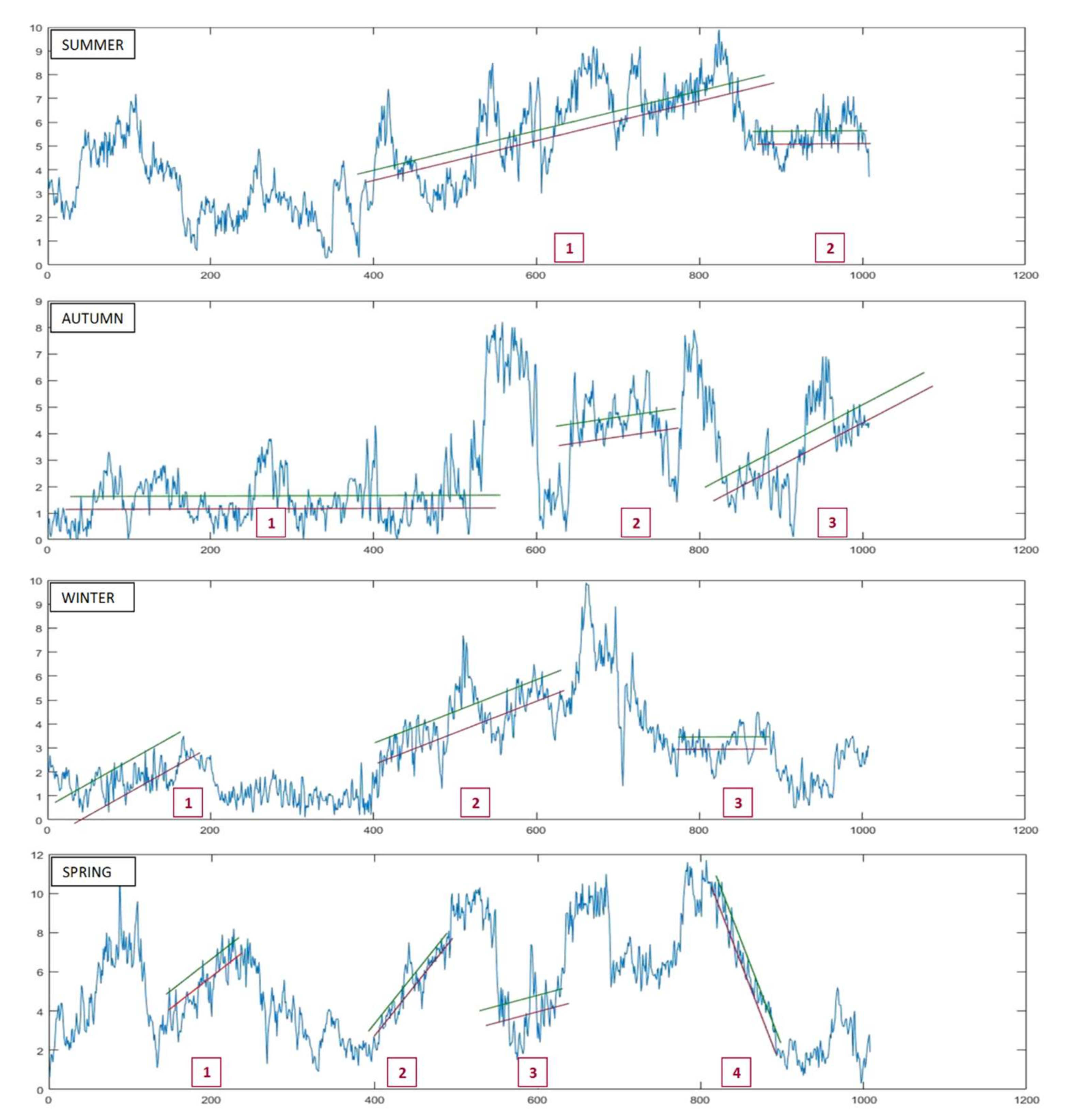
To complete this part of the analysis, some of the most significant trending channels during the four selected weeks are evidenced in Figure 2 (resistance lines in green, support lines in dark red).

As supports and resistances, trending channels may be either horizontal or rising/decreasing. The longer the channel, the more stable is the trend. For example, the first, an up-trending channel during the summer week in Figure 2, shows a difference between the resistance and support line of around 0.4 m/s and lasts more than four hundred values—almost three days. Similarly long is the first trending channel in the autumn week: a horizontal one again with a gap of 0.4 m/s (from 1.2 to 1.6 m/s), long enough to cover almost four days of the week. In this channel, the support line is broken 17 times, creating each time a new minor resistance level, and the resistance line is broken 25 times, creating an equal number of minor support levels. Finally, an additional peculiar characteristic of the analysed wind speed data series is that in many cases, support and resistance lines have slopes that are very similar in magnitude (and opposite in sign) to speed increases and decreases. These are reasonable if considering that the changes in the wind speed are related to physical variations that may occur with the same rapidity in both directions. These characteristics may give useful advice for at least qualitative forecasting of wind speed evolution.

5.2. Candlesticks

Examples of application of the Japanese candlesticks data from both Los Montes del Cierzo and Capo Mele were analysed.

5.2.1. Los Montes del Cierzo—Data Every 10 min

For the Los Montes del Cierzo data series, candlesticks were created using data with 10-min resolution acquired both at 10 m and 2 m above the ground. Each hour (i.e., six values) was converted into a candlestick: the first value as the opening one, the sixth value as the closing one and the minimum/maximum to set the extremes of the candlestick shadows. Thus, for each representative week, 168 candlesticks were drawn.

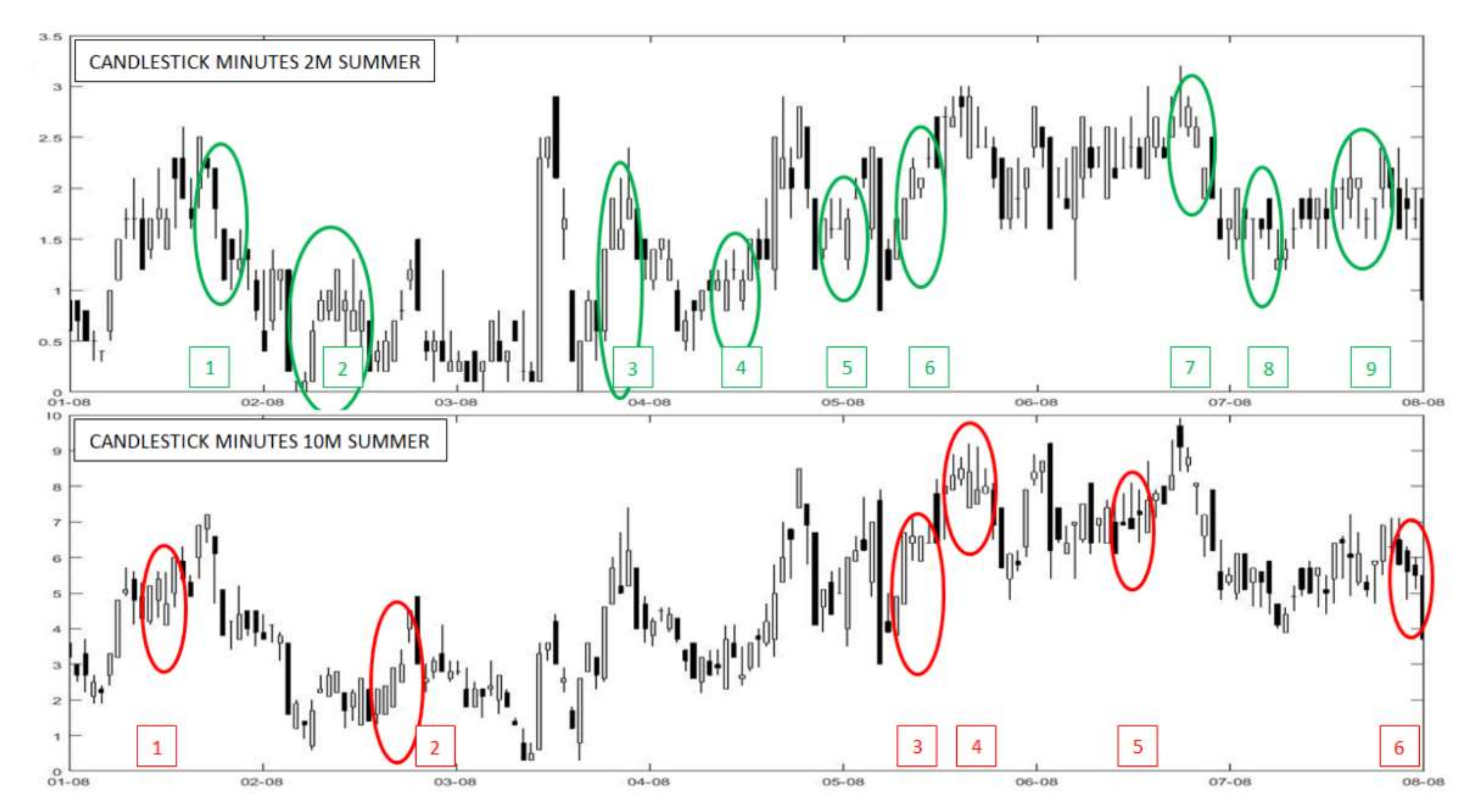
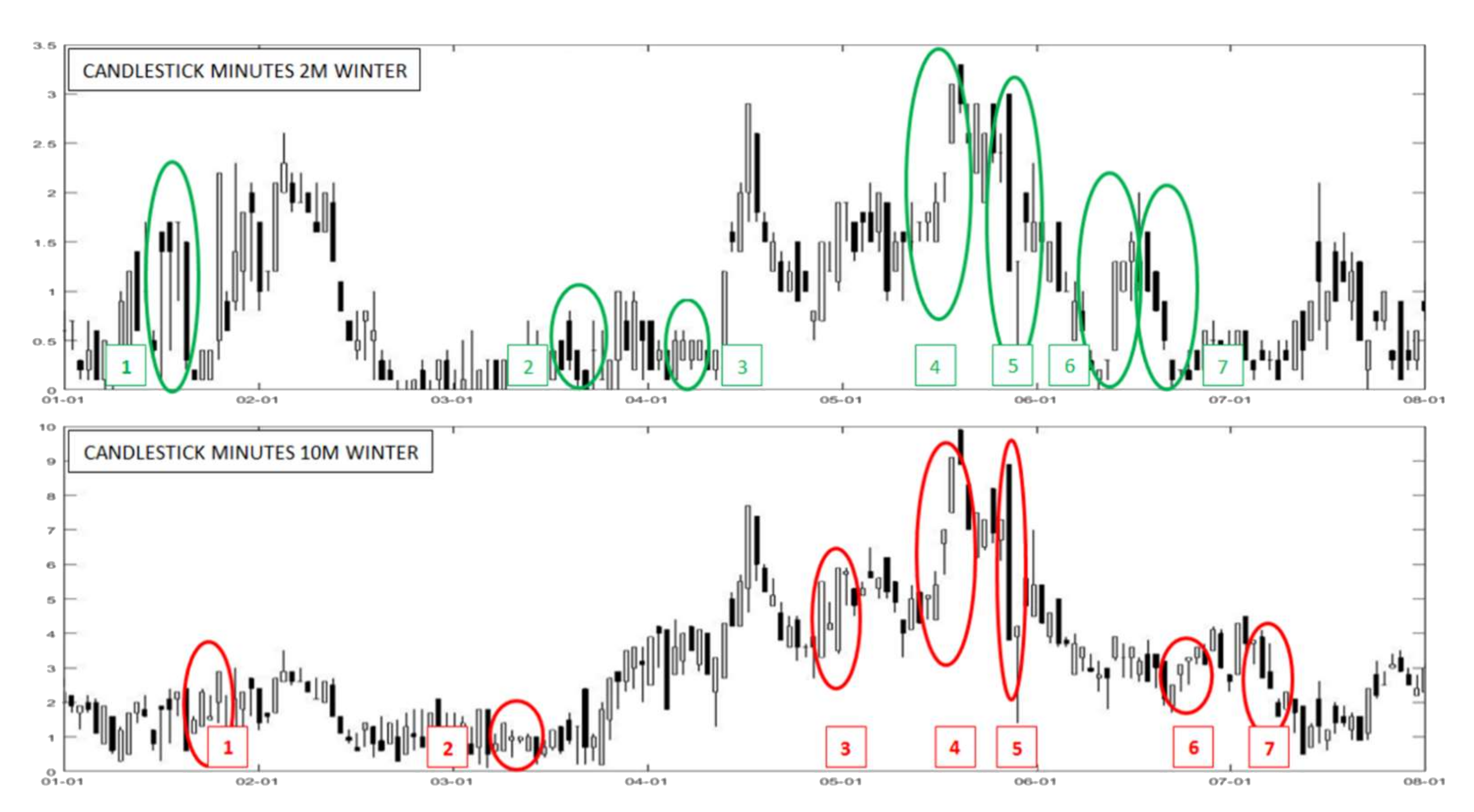
As it was done for the support and resistance lines, peculiar candlesticks trends and patterns (evidenced with coloured ellipses and numbers in the charts) were identified for four weeks, representative of the different seasons. Figure 3 shows the results for the first week of August 2016, for data acquired at both 2 m and 10 m above the ground. Even if it is still a quite low height, the values at 10 m are more representative of the situation that a real wind turbine would encounter; therefore, they will be commented on first and more in-depth. Data at 2 m were added for comparison and to evaluate the modifications in the trends due to the atmospheric boundary layer.

In sets 1–4, white candlesticks are present, meaning that the wind speed closing value was higher than the first values. For single groups and as a whole, this means an increase in wind speed. In one, two (the latter being a perfect example of a “bearish breakaway” pattern) and three, it can also be observed that the bodies of the candlesticks are long and with very short shadows, particularly at the beginning of the group. This gives a clear indication that a trend inversion has just happened, and a “bullish” phase (rise) is starting. On the contrary, in set four, short bodies and long upper shadows can be observed, meaning that the wind speed has reached a plateau and a decrease is likely to happen.

Other candlestick patterns can also be detected, e.g., a “shooting star” followed by a “falling three” centred on August 4th.

In set five, short black bodies with long shadows are initially present, followed by a long white candlestick: wind speed comes from a period of uncertainty (alternated long white and black candlesticks) but—even without difficulties, as evidenced by the long shadows—another rising period begins. On the contrary, in set six, the series of black candlesticks clearly shows the decreasing phase, which could have been expected in advance given the appearance of a long white candlestick followed by a very short one with long shadows.

Moving to the chart related to August 2016 at 2 m above the ground, the wind speed values are obviously much lower, but the qualitative behaviour in terms of rise/decrease is much like the 10-metre case (even if some candlesticks are different in shape or colour). Nine candlestick figures can be identified. Sets one and eight include a. black candlestick only, so wind speed decreases, and both do not have upper shadows. This means that the opening wind speed is the highest one in the time span and thus the wind speed steadily decreased along the hour. Sets 3, 7 and 9 are made by all-white candlesticks; thus the wind speed always increases. Set three shows a possible support level at the beginning and later an incoming turning point: the first two candlesticks have the maximum as their closing value, followed by two candlesticks with long upper shadows, representing that high values were reached in the time period. Then, a long black candlestick closes the rising phase.

Sets from 4 to 7 and 9 all include candlesticks without a body, meaning that the initial and final values were equal. This figure in Japanese is called a “doji”, and its relevance depends on the preceding trends or candlesticks: after a long white candlestick (as in Set 5 and partially in Set 7) a “doji” signals that the increment of the wind speed is going to stop, and the uptrend could be near to the end.

Focusing on trend inversion alone, further “classic” candlesticks and patterns can also be evidenced in the chart: e.g., a “hammer” candlestick is present in the August 1st data and a “bearish engulfing” pattern is present during August 3rd (evident both at 2 m and 10 m).

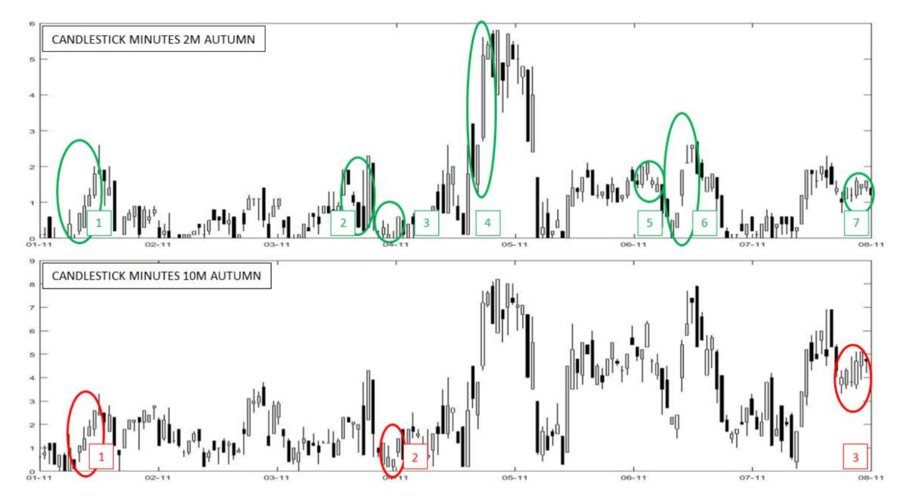
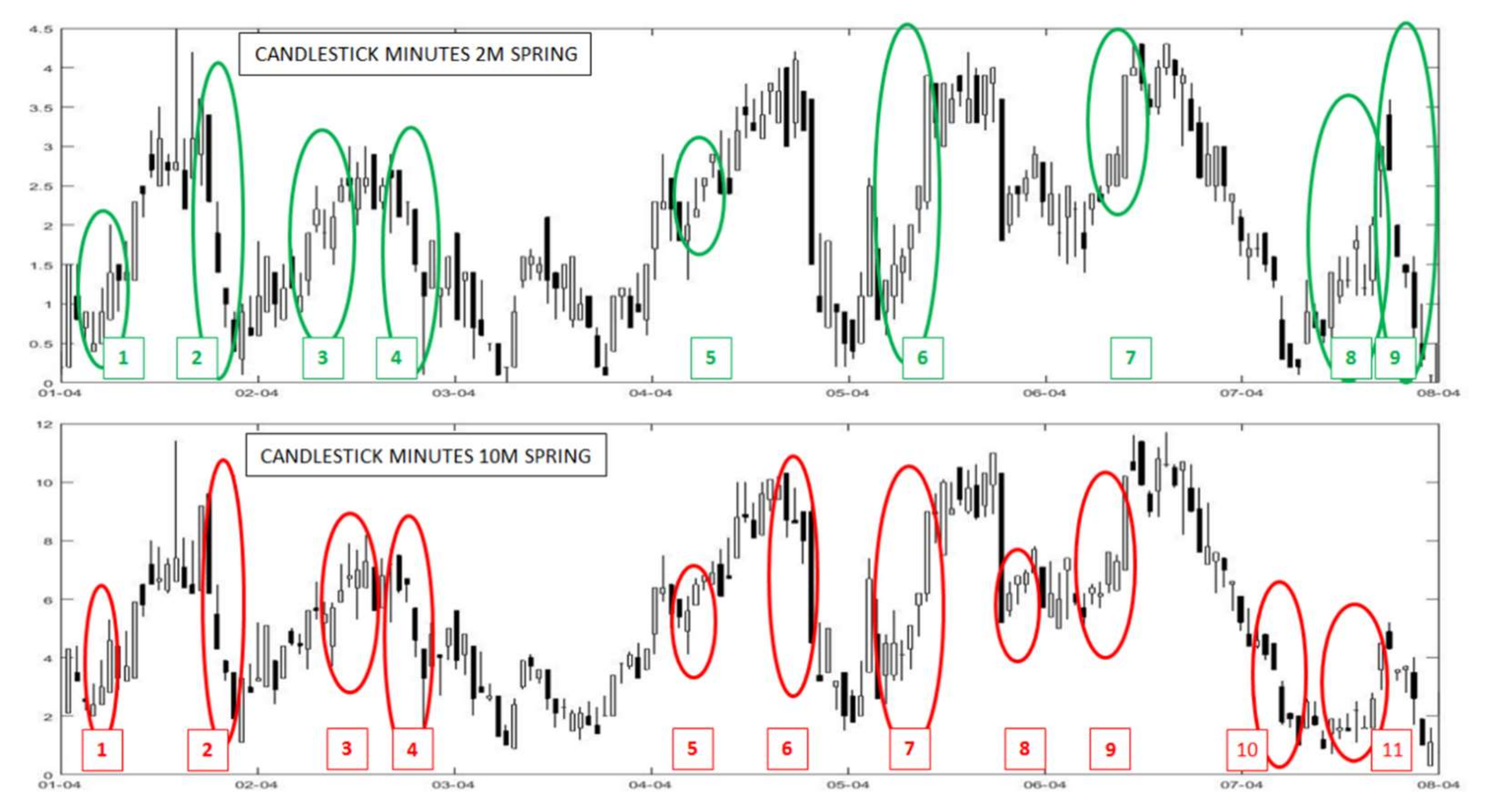
Moving to the other seasons, Figure 4, Figure 5 and Figure 6 show the results for the first week of November 2016 (autumn), January 2017 (winter) and April 2017 (spring), again for data acquired at 10 m and 2 m from the ground. Some significant candlesticks patterns, similar to those already described for summer, are evidenced and numbered in the charts, e.g., set one and set six in the autumn week, 2 m from the ground values, are examples of “three white soldiers”, which is a “bullish” pattern, whilst set two is another “falling three” example. Other sets can be identified in these cases too: e.g., in the autumn week, 10 m from the ground values, a “hanging man” (“bearish” figure) is present immediately before November 2nd.

5.2.2. Capo Mele–Data Every Hour

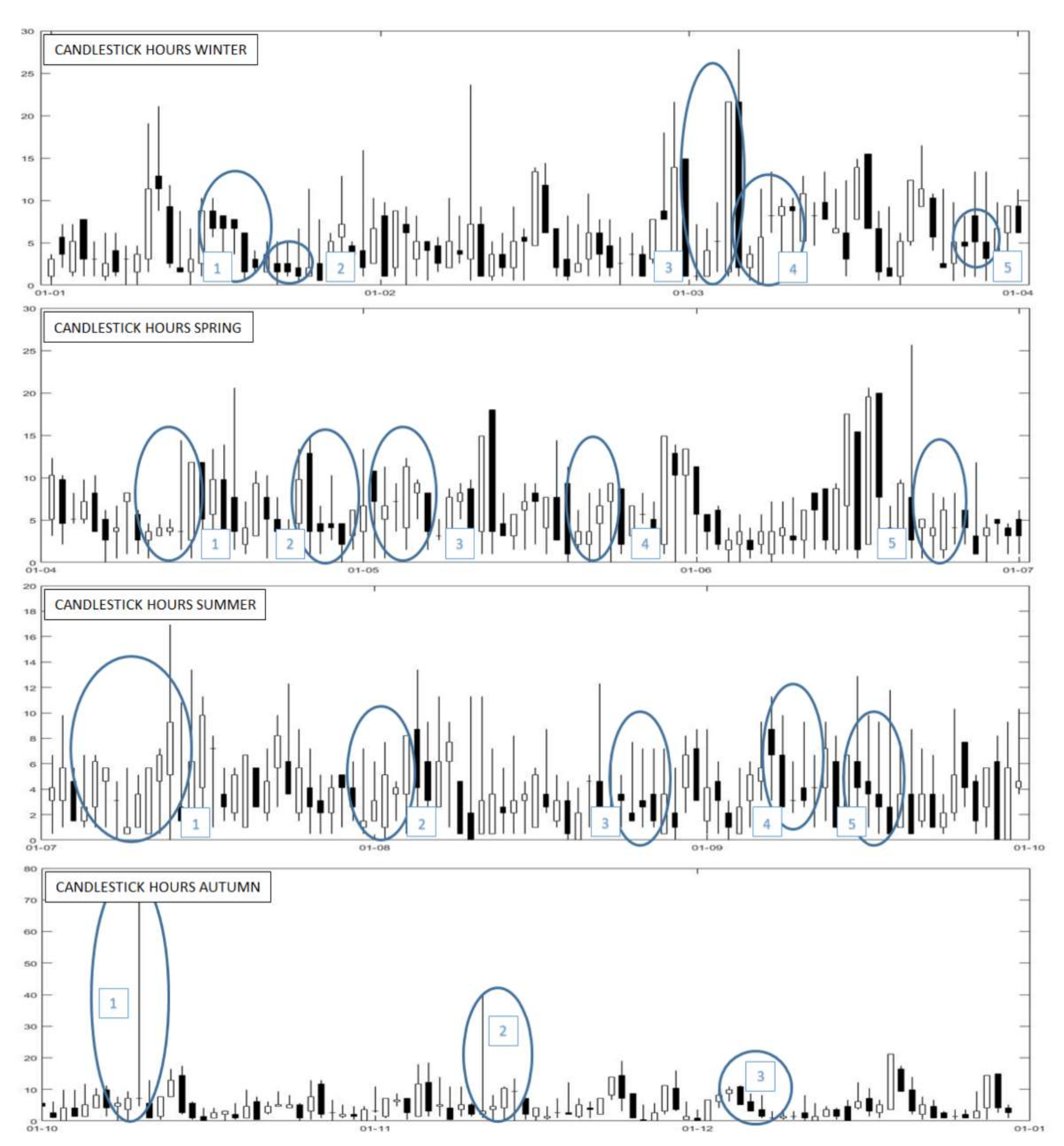
For the Capo Mele location, data are available only with a 60-min time resolution; thus, candlesticks were created on a daily basis and the full year was covered. Conventionally, it was decided to include January, February and March in the “winter” season; April, May and June in “spring”; July, August and September in “summer”; and finally, October, November and December in “autumn”. Representing one day, each candlestick is created from 24 hourly values of wind speed, with the values at the beginning and end of the day as opening and closure values and completed with the minimum and maximum values of the day. As it can be observed from Figure 7, which shows the results, many candlestick patterns can be identified using daily candlesticks too. Some significant sets are evidenced and numbered in the figure; additional ones—e.g., an “evening star” immediately before set one in the winter chart—can also be spotted. Nonetheless, the analysis on an hourly basis is much more useful for the wind energy market because it can offer an indication about inversion points hour-by-hour; thus, as usual, a high time resolution of the data series is beneficial.

Additional occurrences of candlesticks patterns related to inversion, indecision or continuation are reported in Appendix A, Table A1.

5.3. Combination of the Two Techniques

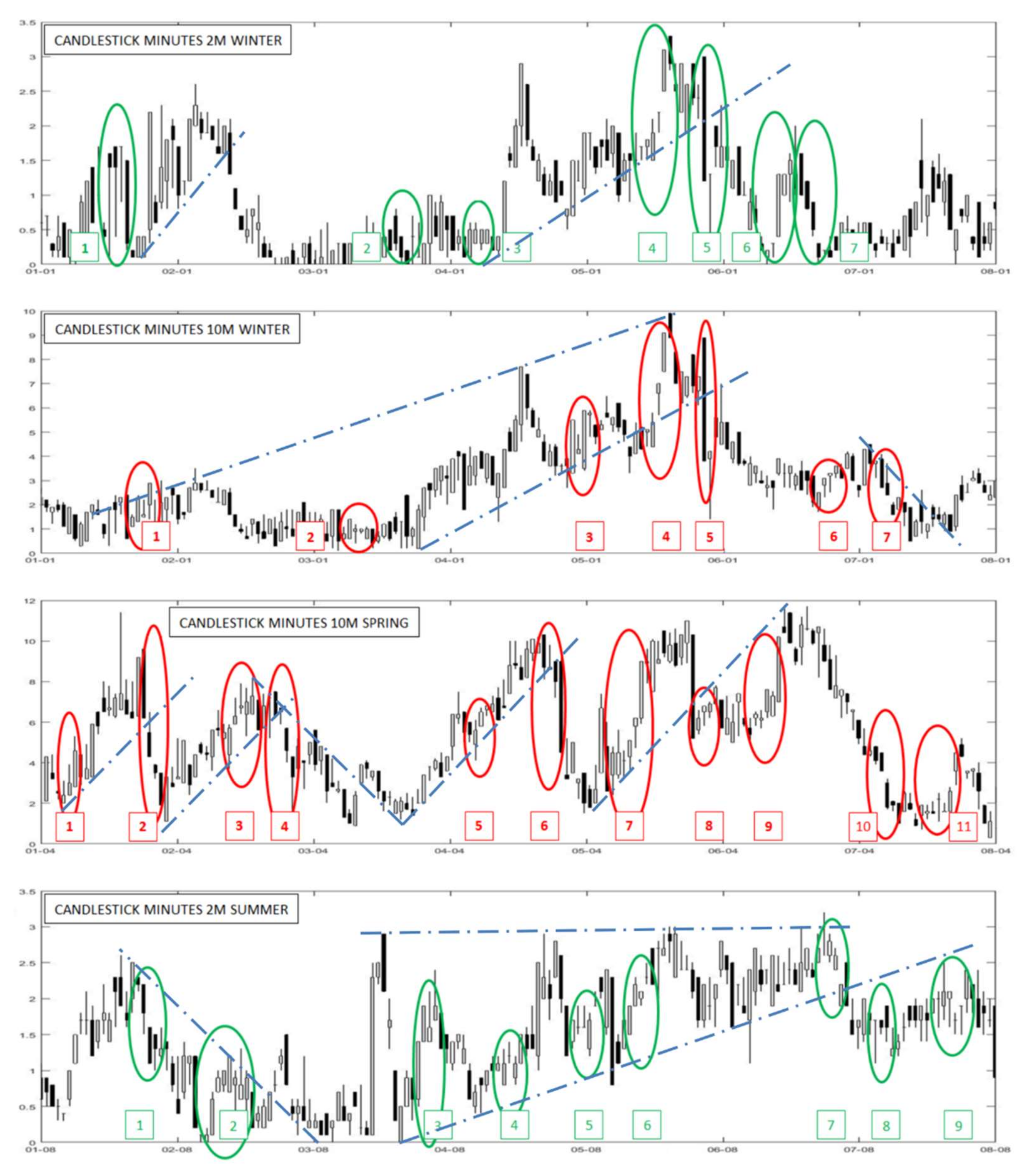
It is also evident from the charts in Figure 3, Figure 4, Figure 5 and Figure 6 that support and resistance lines could also be traced on the candlestick charts in an effective way, i.e., the two techniques can be usefully combined. Figure 8 shows some examples of support and resistance lines traced as dash–dot lines on the same candlestick charts. Again, in many cases, the slope of the rising/decreasing lines is very similar in magnitude (changing in sign), as already commented.

6. Conclusions

The trend lines/trending channels and the candlesticks techniques from the financial “technical analysis” were applied to the analysis of wind speed data series. The aim was to verify if such models can be useful to identify the series patterns and particularly the inversion points. In fact, the latter is critical for all the models that are based on time continuation from past data, and in wind speed, forecasting is among the most used ones. Wind speed data from two locations, one in Spain and one in Italy, were used. The study confirmed that both significant trend lines and classic candlestick patterns can be successfully identified in wind data series. Such indicators are sufficiently detailed in time and can help the forecasting models if data at 10–15-minute resolution are available, so that the analysis, particularly in the candlestick case, can be performed on an hourly basis. On the contrary, if data are available only with an hourly time resolution, relevant features can still be identified; however, the usefulness for the wind energy market is obviously much reduced. Concerning future developments, additional tools of financial technical analysis could be tested (e.g., Heikin–Ashi candlesticks or Renko, Point-and-Figure and Kagi charts; in all cases, considering wind speed data with a high time resolution) to further explore the potentiality of such an approach in enhancing the performances of forecasting models. Moreover, automatic detection of trend lines/trending channels and candlesticks patterns could be implemented and coupled with the other available data in machine learning approaches for forecasting.

References

- Koračin, D.; Belu, R.; Canadillas, B.; Horvath, K.; Vellore, R.; Smith, C.; Jiang, J.; McCord, T. A review of challenges in assessment and forecasting of wind energy resources. Croat Meteorol. J. 2012, 47, 13–33. [Google Scholar]
- Ambach, D.; Vetter, P. Wind speed and power forecasting a review and incorporating asymmetric loss. In Proceedings of the Second International Symposium on Stochastic Models in Reliability Engineering, Life Science and Operations Management, Beer Sheva, Israel, 8–11 February 2016; Volume 1, pp. 115–123. [Google Scholar] [CrossRef]
- Wu, Y.-K.; Hong, J.-S. A literature review of wind forecasting technology in the world. In Proceedings of the IEEE PowerTech Conference, Lausanne, Switzerland, 1–5 July 2007; pp. 504–509, ISBN 9781467399418/16. [Google Scholar]
- Kariniotakis, G. (Ed.) Renewable Energy Forecasting—From Models to Applications, 1st edWoodhead Publishing: London, UK, 2017; ISBN 9780081005057/9780081005040. [Google Scholar]
- Chang, W.-Y. A literature review of wind forecasting methods. J. Power Energ. Eng. 2014, 2, 161–168. [Google Scholar] [CrossRef]
- Foley, A.M.; Leahy, P.G.; Marvuglia, A.; McKeogh, E.J. Current methods and advances in forecasting of wind power generation. Renew Energ. 2012, 37, 1–8. [Google Scholar] [CrossRef] [Green Version]
- Barbosa de Alencar, D.; de Mattos Affonso, C.; Célio Limão de Oliveira, R.; Moya Rodríguez, J.L.; Cabral Leite, J.; Reston Filho, J.C. Different models for forecasting wind power generation: Case Study. Energies 2017, 10, 1976. [Google Scholar] [CrossRef] [Green Version]
- Lawan, S.M.; Abidin, W.A.W.Z.; Chai, W.Y.; Baharun, A.; Masri, T. Different models of wind speed prediction: A comprehensive review. Int. J. Sci. Eng. Res. 2014, 5, 1760–1768. [Google Scholar]
- Lei, M.; Shiyan, L.; Chuanwen, J.; Hongling, L.; Yan, Z. A review on the forecasting of wind speed and generated power. Renew Sust. Energ. Rev. 2009, 13, 915–920. [Google Scholar] [CrossRef]
- Jursa, R.; Rohrig, K. Short-term wind power forecasting using evolutionary algorithms for the automated specification of artificial intelligence models. Int. J. Forecast. 2008, 24, 694–709. [Google Scholar] [CrossRef]
- Wang, X.; Guo, P.; Huang, X. A Review of wind power forecasting models. Energy Proced. 2011, 12, 770–778. [Google Scholar] [CrossRef] [Green Version]
- Soman, S.S.; Zareipour, H.; Malik, O.; Mandal, P. A review of wind power and wind speed forecasting methods with different time horizons. In Proceedings of the North American Power Symposium, Arlington, TX, USA, 26–28 September 2010; pp. 1–8. [Google Scholar] [CrossRef]
- Frediani, M.E.B.; Hopson, T.M.; Hacker, J.P.; Anagnostou, E.N.; Delle Monache, L.; Vandenberghe, F. Object-Based Analog Forecasts for Surface Wind Speed. Mon. Weather Rev. 2017, 145, 5083–5102. [Google Scholar] [CrossRef]
- Caporin, M.; Preś, J. Modelling and forecasting wind speed intensity for weather risk management. Comput. Stat. Data Anal. 2012, 56, 3459–3476. [Google Scholar] [CrossRef] [Green Version]
- Fischer, A.; Montuelle, L.; Mougeot, M.; Picard, D. Statistical learning for wind power: A modeling and stability study towards forecasting. Wind Energy 2017, 20, 2037–2047. [Google Scholar] [CrossRef] [Green Version]
- Habib, A.; Abbassi, R.; Aristizábal, A.J.; Abbassi, A. Forecasting model for wind power integrating least squares support vector machine, singular spectrum analysis, deep belief network, and locality-sensitive hashing. Wind Energy 2020, 23, 235–257. [Google Scholar] [CrossRef]
- Madhiarasan, M.; Louzazni, M. Different forecasting horizons based performance analysis of electricity load forecasting using multilayer perceptron neural network. Forecasting 2021, 3, 49. [Google Scholar] [CrossRef]
- Kannari, L.; Kiljander, J.; Piira, K.; Piippo, J.; Koponen, P. Building heat demand forecasting by training a common machine learning model with physics-based simulator. Forecasting 2021, 3, 19. [Google Scholar] [CrossRef]
- Ogliari, E.; Guilizzoni, M.; Giglio, A.; Pretto, S. Wind power 24-h ahead forecast by an artificial neural network and an hybrid model: Comparison of the predictive performance. Renew. Energ. 2021, 178, 1466–1474. [Google Scholar] [CrossRef]
- Cheng, L.; Zang, H.; Ding, T.; Sun, R.; Wang, M.; Wei, Z.; Sun, G. Ensemble Recurrent Neural Network Based Probabilistic Wind Speed Forecasting Approach. Energies 2018, 11, 1958. [Google Scholar] [CrossRef] [Green Version]
- Zhou, J.; Sun, N.; Jia, B.; Peng, T. A Novel Decomposition-Optimization Model for Short-Term Wind Speed Forecasting. Energies 2018, 11, 1752. [Google Scholar] [CrossRef] [Green Version]
- Stock Charts. Available online: https://www.chart-formations.com/stock-charts/default.aspx (accessed on 9 November 2021).
- Murphy, J.J. Technical Analysis of the Financial Markets: A Comprehensive Guide to Trading Methods and Applications; New York Institute of Finance; Prentice Hall Press: New York, NY, USA, 1999; ISBN 978-0735200661. [Google Scholar]
- Osler, C. Support for Resistance: Technical Analysis and Intraday Exchange Rates. FRBNY Econ. Policy Rev. 2000, 6, 53–68. [Google Scholar]
- Nison, S. Japanese Candlestick Charting Techniques: A Contemporary Guide to the Ancient Investment Techniques of the Far East, 2nd ed.; Prentice Hall Press: Upper Saddle River, NJ, USA, 2001; ISBN 978-0735201811. [Google Scholar]
- Morris, G.L. Candlestick Charting Explained: Timeless Techniques for Trading Stocks and Futures, 3rd ed.; McGraw-Hill: New York, NY, USA, 2006; ISBN 978-0071461542. [Google Scholar]
- StockCharts: Introduction to Candlesticks. Available online: https://school.stockcharts.com/doku.php?id=chart_analysis:introduction_to_candlesticks (accessed on 9 November 2021).
- Kuepper, J. On Investopedia—Advanced Candlestick Patterns. Available online: https://www.investopedia.com/articles/trading/06/advcandlesticks.asp (accessed on 9 November 2021).
- Mitchell, C. On Investopedia—Understanding Basic Candlestick Charts. Available online: https://www.investopedia.com/trading/candlestick-charting-what-is-it (accessed on 9 November 2021).
Figure 1.
Wind speed data series for Los Montes del Cierzo (10 min resolution, for the first weeks of August 2016, November 2016, January 2017 and April 2017, height 10 m above the ground) with some significant examples of support and resistance lines.
Figure 2.
Wind speed data series for Los Montes del Cierzo (10 min resolution, for the first weeks of August 2016, November 2016, January 2017 and April 2017, height of 10 metres above the ground) with some significant examples of trending channels.
Figure 3.
Candlestick chart for Los Montes del Cierzo, hourly resolution, first week of August 2016, at 2 m (top) and 10 m (bottom) above the ground.
Figure 4.
Candlestick chart for Los Montes del Cierzo, hourly resolution, first week of November 2016, at 2 m (top) and 10 m (bottom) above the ground.
Figure 5.
Candlestick chart for Los Montes del Cierzo, hourly resolution, first week of January 2017, at 2 m (top) and 10 m (bottom) above the ground.
Figure 6.
Candlestick chart for Los Montes del Cierzo, hourly resolution, first week of April 2017, at 2 m (top) and 10 m (bottom) above the ground.
Figure 7.
Candlestick chart for Capo Mele data, with daily resolution over a whole year.
Figure 8.
Some examples of identification of trend lines on candlestick charts for Los Montes del Cierzo, hourly resolution.
Publisher’s Note: MDPI stays neutral with regard to jurisdictional claims in published maps and institutional affiliations. |
© 2022 by the authors. Licensee MDPI, Basel, Switzerland. This article is an open access article distributed under the terms and conditions of the Creative Commons Attribution (CC BY) license (https://creativecommons.org/licenses/by/4.0/).
Share and Cite
MDPI and ACS Style
Guilizzoni, M.; Maldonado Eizaguirre, P. Trend Lines and Japanese Candlesticks Applied to the Forecasting of Wind Speed Data Series. Forecasting 2022, 4, 165-181. https://0-doi-org.brum.beds.ac.uk/10.3390/forecast4010009
AMA Style
Guilizzoni M, Maldonado Eizaguirre P. Trend Lines and Japanese Candlesticks Applied to the Forecasting of Wind Speed Data Series. Forecasting. 2022; 4(1):165-181. https://0-doi-org.brum.beds.ac.uk/10.3390/forecast4010009
Chicago/Turabian StyleGuilizzoni, Manfredo, and Paloma Maldonado Eizaguirre. 2022. "Trend Lines and Japanese Candlesticks Applied to the Forecasting of Wind Speed Data Series" Forecasting 4, no. 1: 165-181. https://0-doi-org.brum.beds.ac.uk/10.3390/forecast4010009