
Advances in Time Series Forecasting Development for Power Systems’ Operation with MLOps


1
Institute for Automation of Complex Power Systems, E.ON Energy Research Center, RWTH Aachen University, 52064 Aachen, Germany
2
Center for Digital Energy Aachen, Fraunhofer FIT, 52074 Aachen, Germany
*
Author to whom correspondence should be addressed.
†
Current address: Department of Electrical Engineering, RWTH Aachen University, Mathieustr. 10, 52074 Aachen, Germany.
Forecasting 2022, 4(2), 501-524; https://0-doi-org.brum.beds.ac.uk/10.3390/forecast4020028
Submission received: 18 April 2022
/
Revised: 10 May 2022
/
Accepted: 16 May 2022
/
Published: 26 May 2022
(This article belongs to the Collection Energy Forecasting)
Abstract
:Forecast developers predominantly assess residuals and error statistics when tuning the targeted model’s quality. With that, eventual cost or rewards of the underlying business application are typically not considered in the model development phase. The analysis of the power system wholesale market allows us to translate a time series forecast method’s quality to its respective business value. For instance, near real-time capacity procurement takes place in the wholesale market, which is subject to complex interrelations of system operators’ grid activities and balancing parties’ scheduling behavior. Such forecasting tasks can hardly be solved with model-driven approaches because of the large solution space and non-convexity of the optimization problem. Thus, we generate load forecasts by means of a data-driven based forecasting tool ProLoaF, which we benchmark with state-of-the-art baseline models and the auto-machine learning models auto.arima and Facebook Prophet.
1. Introduction
Active power system management (ASM) rapidly gains importance as energy generation moves closer to the end-consumer in distribution systems, while at the same time consumer loads become more flexible. In this context, new strategies and tools for cost-efficient and thus secure management of the emerging energy flexibility are needed, not only over large distances, in transmission systems, but also in local distribution systems, on the last mile to the energy consumers.
The transmission system operator (TSO) and the distribution system operator (DSO) are the two responsible parties that need to monitor and balance supply and demand and the reliable system operation in their respective zones. A secure overall power supply, however, necessitates the close coordination between them. According to the European TSO–DSO report for ASM [1], short-term forecasting is one of the key components for such coordinated operation. This is because, in comparison to conventional power system operations, today’s and future systems are influenced by intermittent generation. Consequently, they have to deal with uncertain energy schedules in short-term planning.
A perfect up-front scheduling and matching between generation and load becomes impossible. Eventually, any deviation between the predicted system state and the actual generation and load causes costly counter-balancing measures. In this context, this paper deals with the potential reduction of the necessary measures by means of more accurate short-term forecasting under uncertainty. Imperfect forecasts of renewable energy source (RES) feed-in can furthermore lead to more frequent overloading in the transmission system [2]. Such overloading, i.e., the transport of energy above the permissible safety limits of power system devices, are summarized under the term ‘congestion’. In addition to the physical congestion, market and structural congestion also exist, as described in [1]. In simple terms, almost all short-term congestion management decisions are due to forecasting errors, as network operators usually have enough flexibility to mitigate risks at an early stage by means of technical and market-based solutions, such as redispatch.
The study, presented in [2], particularly focuses on the German transmission grid to provide a qualitative evaluation of the forecast errors’ impact on the congestion management process. As a factor of uncertainty, the model includes the wind energy output. Beyond that, it may be useful to not define the uncertainty factors in advance. The reason for this is that, in addition to the significant uncertainty of wind generation, minor fluctuations in the demand itself, as well as other generation sources, will have an impact on the future net load. In this work, we therefore propose not to separately model the uncertainty impact of load fluctuations and generation fluctuations, as they cannot be clearly distinguished.
The suggested forecasting model is designed to learn from historic profiles and reflect the net load changes over time. Here, the changes are associated with spatio-temporal dependencies. We carefully select calendrical, meteorological, and also geographic information from the past and feed this into the presented data-driven model. The configuration of the forecast model parameters, tuning, and evaluation of the model is available as an open-source forecast worker. The probabilistic load forecasting with ProLoaF is an integrated tool of the service-based open-source grid automation platform for network operation of the future (SOGNO) [3].
The noted explanatory variables have high potential to increase the accuracy of the net load forecast, in particular if a high correlation between exogenous factors on the energy consumption is evident. However, as [4] discusses, an inclusion of explanatory variables not only increases the complexity of the forecast models, but also might lead to larger forecasting errors, depending on the quality of the additional variables. The work in [4] further elaborates on how to evaluate RES generation forecasts in particular decision-making contexts. The most important evaluation metrics for multi-variate forecasting are outlined and set into relation of an operation example. These metrics cannot only be used for the ex-post evaluation of the forecast but, likewise, they can be applied as a scoring method during training.
In addition to this scoring metric during training, the metric for selecting the best trained model needs to be chosen carefully in machine learning (ML)-based forecasting practice. One of the most relevant modern introductory works to time series forecasting, i.e., ref. [5], puts forward that a robust and reliable forecast model can only be achieved when the metrics for scoring and selection are distinct. Thus, we consider a selection of established error metrics that we adopt in the present work based on [4,5]. We moreover analyze the metrics’ time dependency and the value of the time-dependent accuracy in the forecasts business context.
In addition, ref. [6] deals with forecasting uncertainty in power system business practices. According to their work, modern deterministic approaches are slowly being replaced by uncertainty forecasting in large parts of the power industry under high-RES conditions. The paper concludes that probabilistic forecasting can achieve a paradigm shift in the way forecasts are used and evaluated. Thus, the value of forecasts can no longer be reduced to simple statistical measures.
A recent review on energy forecasting [7] supports this statement. The majority of (probabilistic) load forecasting papers until 2020 focuses on the improvement of the applied forecast method, whereas findings on the value of the forecast quality in an application context are seldom addressed. Depending on the business application, established forecast quality metrics may not be understood by decision makers, because data analysis might not be their core business. Thus, differences in opinion exist between forecast builders and their users when it comes to labeling a forecast as either good or bad [8].
In the wind energy forecasting domain, in 2011, ref. [9] thoroughly examined the goodness of forecasts from different electricity market agent’s perspectives. The authors define cost objectives of wind farm operators and grid operators and implement these as training criterion for variants of a forecasting model. By comparing the resulting models, they prove that bundling the objective to the training can cause a significant forecast bias, as forecast errors can influence the underlying market, which in turn can open new opportunities to maximize profit for one or another market participant. Thus, although we are interested in the relation of accuracy and value of accuracy, we do not use the value term in the training of the forecast model development in order to mitigate any biases.
As described in [10], system operators in Germany, at least until the end of 2019, still calculated congestion forecasts based on deterministic generation and load forecasts. Here, the short-term unit commitment often needs to be done earlier than 24 h before a possible congestion, as many units are still inflexible and have a minimum ramp-up period. So far, this decision that needs to be made under uncertainty is based on worst-case assumptions with the deterministic load flow. However, although the worst-case analysis is safest from grid operation perspective, it can be too conservative and costly. The next steps, according to [10], are thus to incorporate generation uncertainties into load flow forecasts and grid security processes with scenario studies. Scenario-based uncertainty estimations, however, necessitate expertise on the forecast developer side to identify all significant uncertainty factors and how they change over time. With more and more measurements of explanatory variables over the past years combined with the assumption that the history is representative pf the future, ML models might be capable of learning the impact of varying generation and load on the future net load. In the present work, to develop a model that can learn this known–unknown aspect, we include probabilistic evaluation metrics as training criterion, as an extension to deterministic ones. This allows the forecast user to leverage the knowledge of these uncertain inputs and enables a risk-aware decision in the target business application that reduces costly grid operator interventions, such as balancing and redispatch. This can be done on a uni-variate or multi-variate selection of inputs.
In general, multi-variate probabilistic forecasting gains attention for power system applications as described in [11]. For this, ref. [11] develops forecasting profiles with time variant patterns based on multiple explanatory variables. It is shown that quantile regression forests (QRF) are applicable to dynamically refine the forecasting accuracy as new data are available to update already trained models. It is further shown that multivariate inputs with the dry-bulb temperature as exogenous features outperforms uni-variate ones in the case of short-term electrical load forecasting.
Furthermore, recent studies [12] indicate that deep-learning ML architectures, such as recurrent neural network (RNN) can outperform forecast methods, such as random forest, support vector regression, autoregressive integrated moving average (ARIMA), and vanilla-artificial neural network (ANN) models on electrical load data. Most recently, forecasting competitions such as the M forecasting series with M4 and M5 [13,14,15] have shown that GAMS, XGBoost, STL-decomposed exponential smoothing, prophet, N-BEATS, and LightGBM are at the top of the leader board for current time series forecasting tasks. As described in [15], it is observed that more frequently large multi-model ensembles are built to benefit from the strengths of certain models. As one downside, ensemble methods are costly to operationalize and maintain, as each member of the ensemble increases development and computational efforts, which raises concerns on their practicality in the business context. The authors in [15] further elaborate that the trend of combining forecast models is expected to continue as large computational resources become more accessible and tools for automatic model selection and tuning, the so called autoML, continue to improve. Thus, in this paper, we focus on auto-tuning in ML-based forecasting techniques that could be necessary to rapidly adapt in business environments with complex forecasting tasks. This trend would allow for the separation of the forecast model development that should be considered as “off-the-shelf” to be utilized in production. Although the RNN that is developed in [12] generates predictive intervals, a scenario-based stochastic optimization step is added to determine the economic value of the forecast accuracy. A particular strength of the generation of prediction intervals with the selection of scoring metrics is that the generation of the forecast distribution can flexibly be selected to be either parametric or non-parametric.
In [16], we evaluate the impact of the scoring methods on the resulting prediction intervals and show that for electrical loads at the sub-transmission level, both scoring methods, with Gaussian distribution parameters and quantiles, can be used interchangeably. In particular, ref. [16] introduces an encoder-decoder architecture, i.e., a sub-category of RNN, in which the most salient patterns of the input sequence are passed through a context vector to create a prediction sequence (sequence to sequence learning neural networks (Seq2Seq)). This concept, first published in the pioneering work in [17], originates from the natural language processing domain and is shown to be applicable for time series forecasts [16].
The Seq2Seq model and further ML model candidates that are the most promising ones to solve supervised-learning problems were recently benchmarked for energy load forecasting purposes in [18]. The work concludes that the encoder-decoder model outperforms simple RNN, vanilla-ANN-, xgboost- [19], QRF- [4], persistence-, and ARIMA [20] models.
ProLoaF has been designed to set practices to develop, deploy, and maintain the Seq2Seq model as a robust PyTorch-based RNN model for a rapid uptake of recent ML- based forecasting techniques for energy time series. Bringing the tool into operational context is key to proof portability, maintainability, scalability, and trust in ML-models and is a prerequisite to bring the most recent advances from research into practice, into the control rooms of today’s power system operators.
In summary, in our study we shed light on the system operators need to forecast day-ahead to near-real-time under uncertainty. We study probabilistic predictions of the system load of the German TSO, 50 Hertz transmission (50 HzT). The chosen system is particularly challenging for load forecasters due to a non-negligible impact of renewable energy uncertainties. We then compare the resulting forecasts of ProLoaF with the system operator’s own published forecasts and the open source automated machine-learning forecasts from auto.arima and Prophet [21] using the actual day-ahead prices.
The forecast evaluation based on established forecast error statistics on one side, and the economic valuation of the applied forecast on the other side, is conducted on out-of-sample predictions for the period July to December 2021.
The main contributions of the paper are as follows:
- i.
- We implement a probabilistic short-term forecasting model based on previous work, which we extend by new scoring and tuning methods,
- ii.
- We compare established forecasting models from research and the TSO’s published forecast from production by means of the sum of time-varying cost for all forecast deviations,
- iii
- We integrate the resulting forecast time series into a day-ahead operations framework and thoroughly discuss the quality of grid state forecasts in the chosen operational environment, and
- iv.
- Finally, we formulate a list of considerations to contrast the model’s scalability, maintainability, and trust, which were in focus during the open-source development of ProLoaF.
2. Methodology
In electric power systems with heavy RES penetration, short term load forecasting (STLF) is applied to the generation and load side, to ultimately determine the net load. The net load is given as the total load in one balancing zone, that is, one transmission system control area, and there is no further knowledge on the underlying grid.
2.1. Statistical Forecast Evaluation Metrics
During ex-post evaluation, STLF quality can be expressed with error measures describing the point forecast deviation (accuracy). To quantify the accuracy, in this paper, we use the MSE, RMSE, and MASE. The PLF, however, also necessitates a thorough analysis of the error distribution (certainty) [22]. For instance, with the QS, PICP, and MIS, we can quantify whether a predicted confidence band is sharp and reliable [23]. In the following, we provide the interpretation and characterization of each metric in the time series forecasting context:
- -
- MSE: Quantifies the squared distance of the expected value from the target variable , averaged over the prediction horizon from to . This indicator reflects both the bias and variance of the predicted time-series with respect to the observed one. As such, forecasters seek to minimize it. The MSE is strictly positive and takes the squared scale of the observed data.
- -
- RMSE: The positive square root of the MSE describes, in essence, the same information but is more sensitive to outliers, as larger errors have a disproportionately large effect on it. Forecasters seek to minimize it. The RMSE is strictly positive and takes the scale of the observed data.
- -
- MASE: Averages positive and negative forecast errors equally, irrespective of the scale of the observed data. Forecasters seek to minimize it, as values smaller than one indicate that the given method outperforms an in-sample naïve persistence forecast.
- -
- QS: Reflects a balanced calibration of quantile estimates , penalizing deviations proportionally to their amplitude. Forecasters seek to minimize it. Here, q describes the probability that the observation lies within the quantile and F is the cumulative distribution function (CDF) of the observed data [24].
- -
- PICP: Quantifies the unconditional prevalence of observed data that lie within the considered PI. The PI, in turn, indicates a lower and upper limit within which we expect the target variable to be. The is a commonly used significance level. As a high PICP implies a higher reliability, forecasters seek to maximize it. The metric is given in percent.
- -
- MIS: Evaluates the quality of produced prediction intervals on a predefined significance level. The average interval score [23] grows marginally with the sharpness [23]. By adding penalties on any positive or negative observation outside of the PI, the MIS gives a balanced calibration measure over the prediction horizon from to . Thus, it reflects how tightly the predicted distribution covers the actual observation.
For a detailed definition of the metrics applied, we refer to [16].
2.2. Forecast Implementation
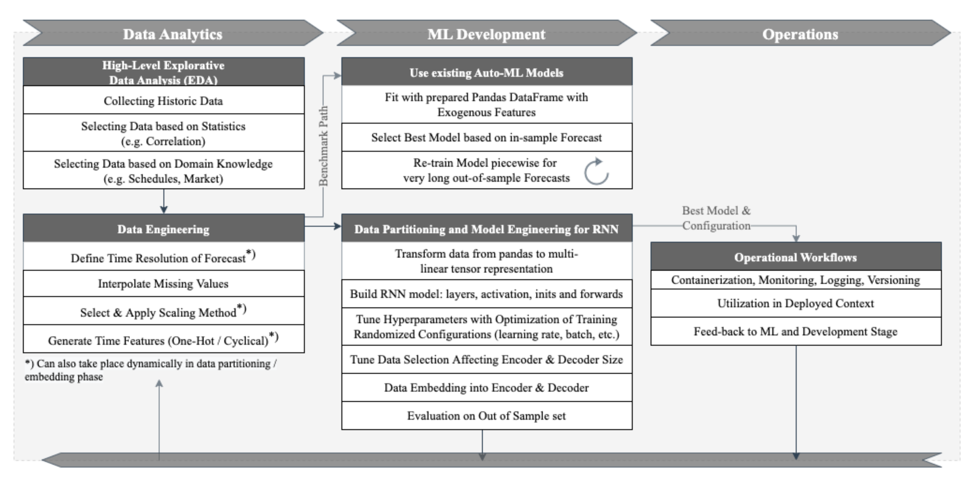
First, we developed a naïve persistence approach with and without seasonal decomposition, as described in [5,25]. Because the RNN outperformed the naïve models with a 50% smaller RMSE than the baseline model, as shown in [16], more advanced regression based methods were selected to benchmark the RNN in this study. Figure 1 shows the selected machine learning workflow, starting with EDA towards development and operation of the forecast model.
2.2.1. Data Pre-Processing
In the EDA, we consider explanatory variables such as the historic local generation, both fossil-based and renewables, historic temperatures, and the historic generation forecasts. As the data are collected from different data sources, adjustments are made to ensure that the timestamps are corrected depending on the timezones. Average and trend elements are used to interpolate larger periods of missing values, such as multiple days. For missing values of few timesteps, the piecewise cubic Hermite interpolating polynomial (PCHIP) method is applied. The frequency of the underlying time series data can flexibly be interpolated or extrapolated to, e.g., daily, hourly, or quarter-hourly values. Because some forecasting methods, such as NN, can be sensitive to unscaled data, ProLoaF provides a single configuration step to apply the most common scaling methods—robust scaling, standard scaling, and minimum-maximum scaling—provided by scikit-learn in Python. We add features describing the hour of the day and day of the week as cyclical time series by encoding the date-time information to sine and cosine elements. These dummy variables are the minimal input required to embed the time-awareness for the recent past and forecast horizon steps. In a next step, we create the dataset with sliding windows of pre-defined window sizes with configurable step sizes. To keep the dataset creation as dynamic as possible, the window size is designed as a configurable optimization parameter. Using PyTorch, we apply all data preparation tasks except the data collection during run-time on the tensor data. The selected preparation steps can also be applied to the underlying pandas DataFrame, which is used as an input for the autoML methods auto.arima and prophet. The data engineering methods, including feature generation, are not further discussed in depth in this paper, as time series feature generation is a topic on its own that already builds largely on helpers, such as [26], to extract features from the inputs.
2.2.2. Auto-ML Model: auto.arima
We select an ARIMA model with seasonal order and exogenous variables [5] and use the Python module to fit ARIMA models with statsmodel [20]. For parameterization, we generate the search space and auto-detect the best performing order configuration of the regression coefficients with the auto.arima algorithm [27]. The model performance is measured with AIC, which is an estimator of the prediction error of statistical models for in-sample tests.
The PI is generated ex-post with the standard deviation of the residuals , where is the prediction target, and is the predicted variable at time step t in sample n of in total N in-sample predictions.
In a next step, we obtain the maximum and minimum value in the prediction interval
where denotes the quantile of the distribution with probability p. Here, the assumption is made that the distribution of errors is standard normal, and thus the confidence band is generated symmetrically around the mean prediction .
Given large sample sets, the Python package statsmodels will quickly cause a high computational burden in terms of storage capacity limitations when the whole sample set is being used to fit a seasonal auto.arima model with exogenous features. In [28], it is shown that the prediction accuracy does not significantly improve with larger sample sizes, independent of the prediction horizon. For this, the RMSE was compared with ARIMA models with incrementally growing sample sizes, starting from 50 to 2200 samples. In training, we limit the sample size to fixed steps. This equals three months with four weeks each in hourly steps. Additionally, we implement a re-fitting procedure for the auto.arima model to predict out-of-sample test data. This means a re-calibration of the model coefficients based on the already trained model. More precisely, we iteratively extend the in-sample data, as the sliding-window propagates through the new incoming data. This procedure replicates an online learning mechanism that would be realized in a deployment context.
2.2.3. Auto-ML Model: Facebook Prophet
With Prophet, there exists yet another forecasting project dedicated to time series predictions. It is available for Python and R developers. Prophet has the target to be a forecasting option that shall be applicable in businesses without the necessity to train the staff in time series methods. In addition, a large variety of forecasting problems shall be solvable, such that a wide range of businesses can be served. In [21], the actual problem of scale in time series forecasting is identified to be the sheer variety of forecasting problems and the trust in the large number of produced forecasts. In contrast, according to [21], computational and infrastructural issues have turned out to be less relevant barriers in this context. Prophet was meant to be a merge of statistical and judgmental forecasts. It is built on a decomposed time series model with three main components, i.e., trend, seasonality, and holidays. Any pattern that is not captured by these three main components falls under the term of idiosyncratic changes that are subject to this specific time series problem. As this particular effect is not captured by the model, it is measurable as one component in the forecasting errors. The Prophet forecasts in this paper are generated with default settings, i.e., a linear growth term, no change points, auto-detection of time series seasonality on yearly, weekly, and daily basis, no holiday embedding, and an additive seasonality.
with
and
in which
Here, g(t) is the trend function, which models non-periodic changes in the value of the time series, and s(t) represents periodic changes (e.g., weekly and yearly seasonality) and is modeled with a standard Fourier series with smoothed seasonal effects, which is described in further detail in [21]. The term denotes the carrying capacity, k is the growth rate, and m describes the offset. The term P is the periodicity that can be set by the forecaster or alternatively will be automatically detected from the data, using typical periods like years, weeks, and days. The coefficients and , which are fitted to the seasonality vector , are modeled per default with .
To fetch upper and lower prediction bounds, , Prophet assumes that the average frequency and magnitude of trend changes in the future will be a re-occurrence of historic observations. The PI is, thus, a projection of the observed errors. This step is similar to our approach for the generation of PIs for the auto.arima model. In the case of Prophet, the number of simulated samples from the posterior predictive distribution that is used to estimate uncertainty intervals is set to 1000 per default.
The method is particularly applicable to data with strong seasonal effects and several seasons of historical data, which is the case for the electrical load profiles, presented in Section 3. Re-calibration is not needed for the Prophet model, as long as trend and seasonal components do not significantly change over the time.
2.2.4. Encoder-Decoder RNN
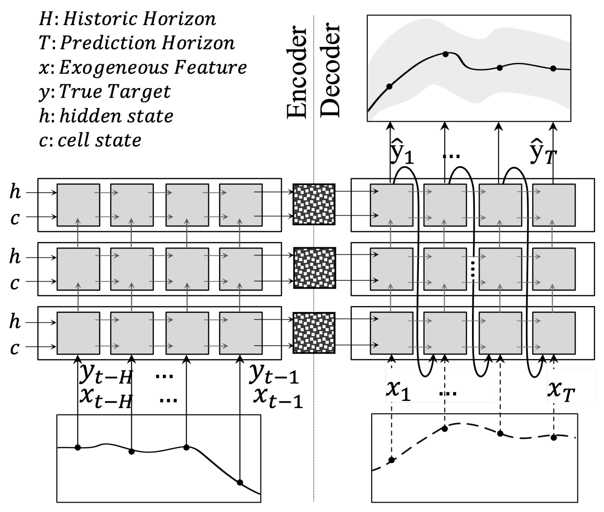
The recurrent neural network model in [16] is designed to process an input sequence of lagged values to produce a new sequence of predictive distributions of the target variable. Its strength lies in processing both explanatory and explained variables in a sequence-dependent (here: time-dependent) context. Using recurrent units (of which commonly known types are LSTM and GRU), long-term effects of historic events can generate an influence on the predicted sequence. This method relies on the fact that observations of the past can lead to a change in the explained variable further ahead in time. Optimally, any salient historic feature should be passed through hidden states to be compressed into a context vector (see Figure 2). In this stage, each generated output from the previous time step is fed into the next time step. Together with the earlier produced context vector from the encoder, the decoder generates as many outputs as variables present in the selected loss function.
We select QS as the loss function because it is non-parametric. The advantage of such distribution is that no assumption about the shape of the residuals is needed.
The forecast model produces and in such a way that the QS on pre-defined quantiles is minimized. By applying the Huber norm to the pinball loss, we obtain a smoothed, approximated quantile score during training. A quantile indicates the probability P for which the target random variable y occurs within it. Given the CDF F of y, the quantile is defined as
The approximated quantile score quantifies whether lies within the estimate of , given the true values , according to
with
where
and
The Huber term is required, to guarantee differentiability, when the prediction errors are close to or equal to zero, as described in [18]. The threshold is set to a number close to zero.
Until recently, grid search and random search were the most common hyperparameter optimization algorithms applied in machine learning. The RNN in [16] is parametrized with a combination of random search and manual selection. For better scaling behavior, we extend the existing method with the integrated tuning algorithm Optuna [29]. The automated hyperparameter search allows testing a large set of parameter combinations in a time-efficient manner, collected in one study. The TPE memorizes achieved objectives within one study and suggests new parameters with higher improvement probability in the next trial.
To regularize the training steps, early stopping is implemented between the optimization steps, such that over-fitting will not occur. For this, a decrease in training loss with simultaneous increase of the validation loss is monitored. Any such case is stopped after a pre-defined number of epochs (the so-called patience).
3. Numerical Results
3.1. Operational Planning Context
The day ahead market closes at 12:00 midday prior to the real-time system operation [30]. Subsequently, multiple phases of preventive redispatch can be necessary in each trading zone, as physical constraints might necessitate a reduction in the flow in certain parts of the grid. A matching counter-balance on the other side of the congestion will then be determined in this process. As described in [30], redispatch is currently done cost-based, i.e., compensation of cost that participating units incurred to change their operating states for the sake of system security.
Figure 3 shows the sequence of processes that take place to settle any imbalances between supply and demand while resolving potential congestion in the respective systems.
In the future, any kind of unit, including RES, that is larger than 100 kW, will participate in these redispatch measures on a market-based mechanism. This means that buy and sell decisions have to be made based on bids in these very short-term markets to balance or even counter-balance any mismatch in the operational planning that is quantifiable by forecast errors. We summarize the whole set of decisions under the terminology remedial actions. To evaluate the impact of accurate load forecasting for these remedial actions, we analyze the remaining forecast errors from day-ahead, two hours prior to the gate closure time of the market. This setting is congruent with the publishing time of the system operator’s day-ahead forecast that is determined in the Commission Regulation (EU) No 543/2013 Article 6.1.A and 6.2.B. The published profiles are openly accessible on the ENTSO-E Transparency Platform every day at 10:00 a.m., in the case of a German control zone.
3.2. Case Study and Data
In this study we use the ENTSO-E Transparency Platform to collect the actual total load (see Article 6.1.A), the day-ahead total load forecast (6.1.B), the aggregated generation per type (Article 16.1.B and C), and the day-ahead generation forecasts for wind and solar (Article 14.1.D). The collected data can be distinguished into actual measurements, given in Table 1, and day-ahead predictions, given in Table 2. In addition, we use the published day-ahead prices for the bidding zone DE-LU, which is the price for the 50 HzT area for every market time unit according to Article 12.1.D.
The electricity in the 50 HzT transmission system comes from interconnection hubs, distribution grids, fossil fueled conventional power plants, wind turbines, PV, and a minor share of other power plants. Currently, the output of approximately 36% of wind power capacity installed in Germany is fed into 50 HzT grid, which is why we select that system for our case study, as an example of a highly uncertain net load prediction task. From the pure numeric perspective, as shown in Figure 4 and documented in [32], 60% of the end consumption capacity, i.e., roughly 100 TWh, is available from 60 TWh renewable sources.
The actual total load per bidding zone per market time unit is equal to the sum of power generated by plants on both TSO and DSO networks, from which the export and import of exchanges on interconnections between neighboring bidding zones is subtracted.
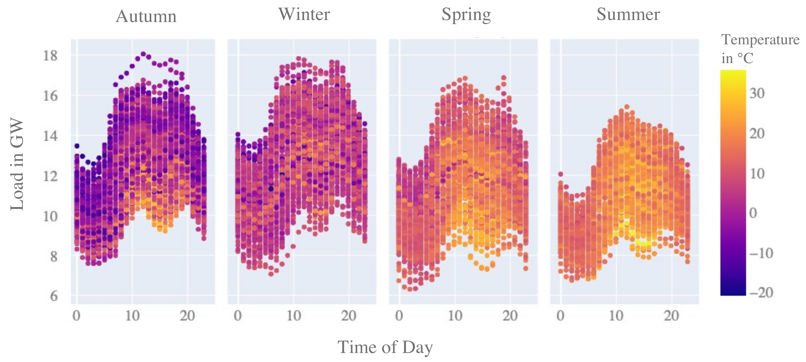
To have a proxy exogenous variable of the ambient temperature changes, we choose the temperature measurement point in Erfurt, i.e., the capital city in the state of Thuringia, which is central Germany. This measurement is located in the southern-west corner of the control zone under study. The correlation between the zonal load and this temperature measurement point is . On average, according to the climate report in [33], the climate in Germany typically is and will be 9 C in spring (March to May), 17.7 C in summer (June to August), 9.9 C in autumn (September to November) and 1.9 C in winter (December to February) in the years 2021–2050. At the chosen measurement point, the average temperature measurements (given the open data published by DWD from October 2018 to December 2021) are 8.15 C in spring, 18.52 C in summer, 10.01 C in autumn, and 2.54 C during winter. In Figure 5, we visualize the seasonal differences in the load patterns averaged per hour of day. During summer, with higher temperatures, the residual load decreases, and vice versa. Reasons for the higher residual load during winter can be electric lighting and heating on the load side, but it is most importantly due to the lower in-feed of PV sourced energy on the generation side.
3.3. Correlation Effect
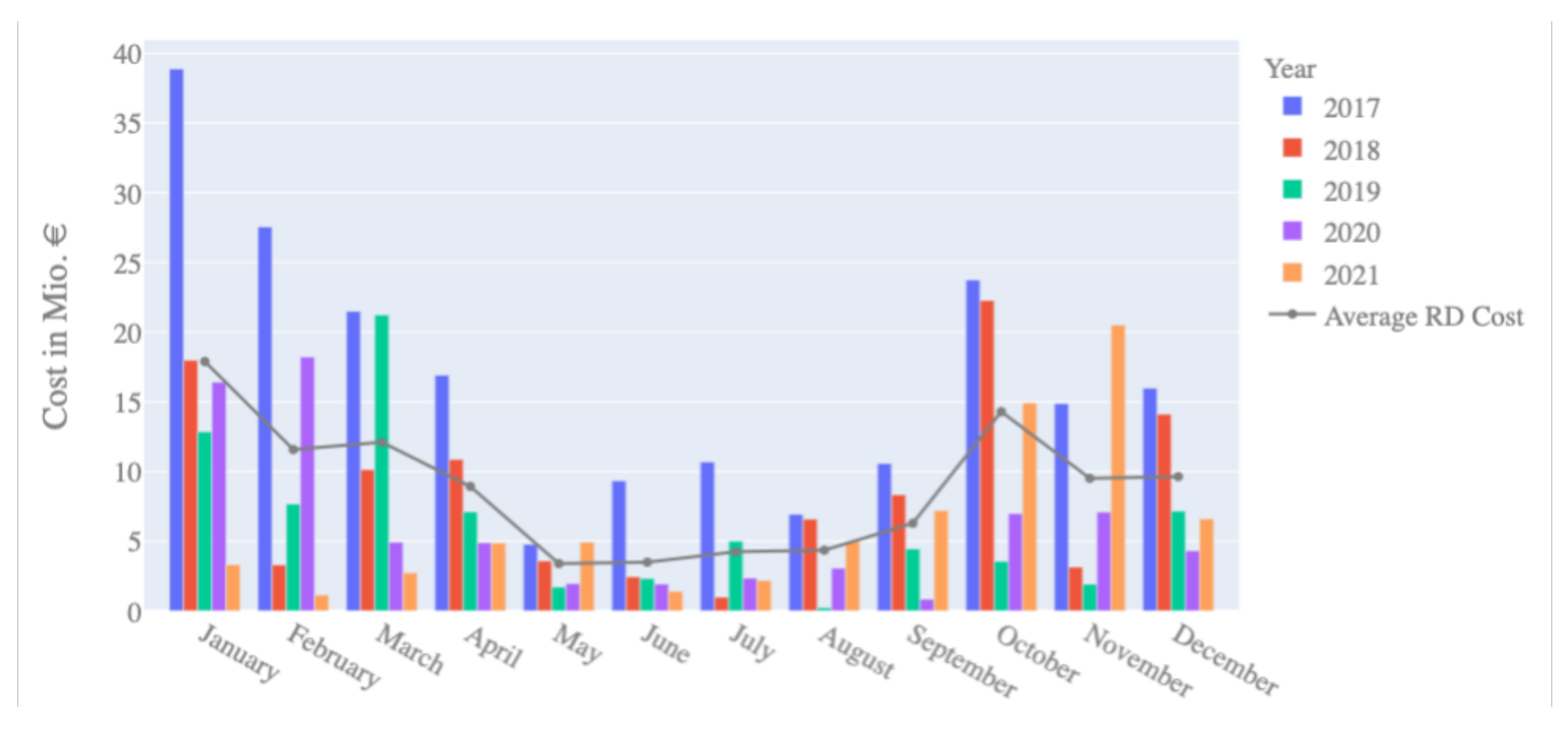
In accordance with Art. 2 (26) of EU Regulation 543/2013, the costs for redispatch measures in Germany include the costs of multilateral remedial actions, interruptible loads, feed-in management of RES, and activation of reserve power. So far, there is no legal basis concerning the compensation for the settlement of re-dispatched units. The 50 HzT system publishes the cost values per year, which is the sum of all compensated costs, via the Transparency Platform. Figure 6 shows the cost development over the years per month. Despite yearly fluctuations, it is evident that during the summer months, on average, fewer redispatch costs are incurred. As congestion occurs when the physical limits are reached, it can be expected that the higher net load in autumn and winter periods results in more frequent critical operation states. This observation underlines the importance that forecasting models, trained with a large set of seasonal data, need to perform as accurately as possible for critical winter days in high net load situations to mitigate high redispatch costs. Lower costs can be achieved with more economic remedial actions as early as possible.
One target of this study is to compare the suggested deep learning algorithm for day-ahead forecasting with the forecast performance of the system operator’s forecast model. With our analysis, we notice that the day-ahead predictions, as published by the system operator on the Transparency Platform, show a significant upward offset of, on average, 1 GW, compared to the published net load values. One reason for this can be that the currently applied prediction model is intentionally set to be conservative, as introduced in Section 1. An additional reason is that the data point for the actual net load (6.1.A) includes net energy imports and exports, whereas the data point of the day-ahead forecast (6.1.B) may not include these. As Figure 4 shows, the 50 HzT system is usually exporting more energy than it imports. The exported energy is subtracted from the net load and thus results in a lower actual net load for this system.
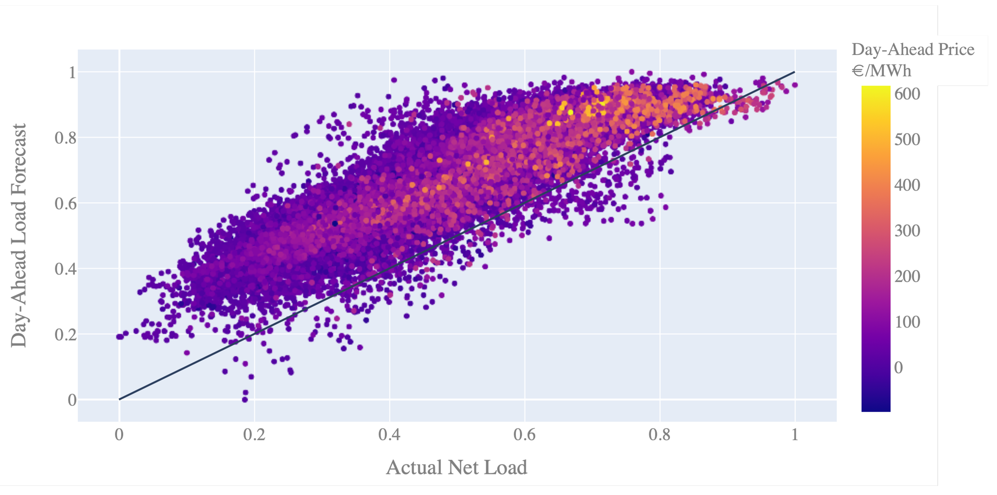
The scatter plot of the day-ahead forecast values against the actual load shows this effect in Figure 7. Furthermore, we see that “high net load” situations are those times that cause high day-ahead prices. Thus, economically efficient decisions could be made with forecast models that are more accurate or less conservative in these cases. This is what we can also see in the scatter plot in Figure 7, as the day-ahead forecast residuals decrease and appear closer to the line, indicating more accurate predictions. A reason for this is most probably that in high net load situations, no further export from the balancing zone to neighboring zones will occur. At the same time, this shows that the deployed forecasting model that is used to publish the open day-ahead forecasts probably has scaled residuals in the range of 0.2, which we can see based on the chosen grid resolution in the plot. However, as it is not clear from the open data platform what further aspects play into a potential correction of the forecast reference, we do no modify or correct the day-ahead forecast data given by the system operator.
3.4. Data Pre-Processing
The grid data, i.e., hourly load and generation profiles for the whole control zone, are split at a 70:15:15 ratio for training, validation, and testing, respectively. The explanatory features are summarized as follows:
- -
- Actual load,
- -
- Actual and forecasted PV and wind energy production,
- -
- Actual local energy generation (conventional Fossil and Other RES),
- -
- Actual temperature,
- -
- Dummy variable for day of the week,
- -
- Dummy variable for hour of day and month of the year (cyclic coding as sine and cosine).
All models are trained with scaled data. For scaling, we use the Minimum-Maximum Scaler function by the pre-processing module scikit-learn v1.0.2 for Python, which can be formulated as follows:
We apply the scaling on all input features and the target variable. A particular advantage of this scaler is that the original distribution of the data is not distorted by the scaling process. However, due to its sensitivity to outliers, other more robust scaling options could be considered depending on the data.
3.5. Model Parameterization
For the auto.arima model, we compare models with and without seasonal parameters and exogenous features. The auto.arima algorithm iterates through tests with incremental changes of the internal auto-regressive and differential coefficients. The resulting model configuration that is the best found solution for each of the ARIMA specifications is given in Table 3. The best model, with the lowest AIC, is the SARIMAX model with exogenous features and a daily seasonality.
Prophet is trained with the whole set of training data, and no further parametrization is done, compared to the default setting as described in Section 2.2.3.
For the ProLoaF RNN, we conduct an automated hyper parameter search optimization with the pre-defined search space that is given in Table 4. As a regularization step, a drop-out rate of 0.2 is applied between layers. Both gated recurrent unit (GRU) and long-short-term memory unit (LSTM) cells were tested. The LSTM based model performed insignificantly better than the GRU based one. Having a lower score on the second digit only after the second decimal point, it is chosen as the best model in this study. The training is interrupted after max. 100 epochs. As an optimizer, we choose per default ADAM, which is further described in [34]. We further apply leaky rectified linear units as an activation function with a slope set to 0.1.
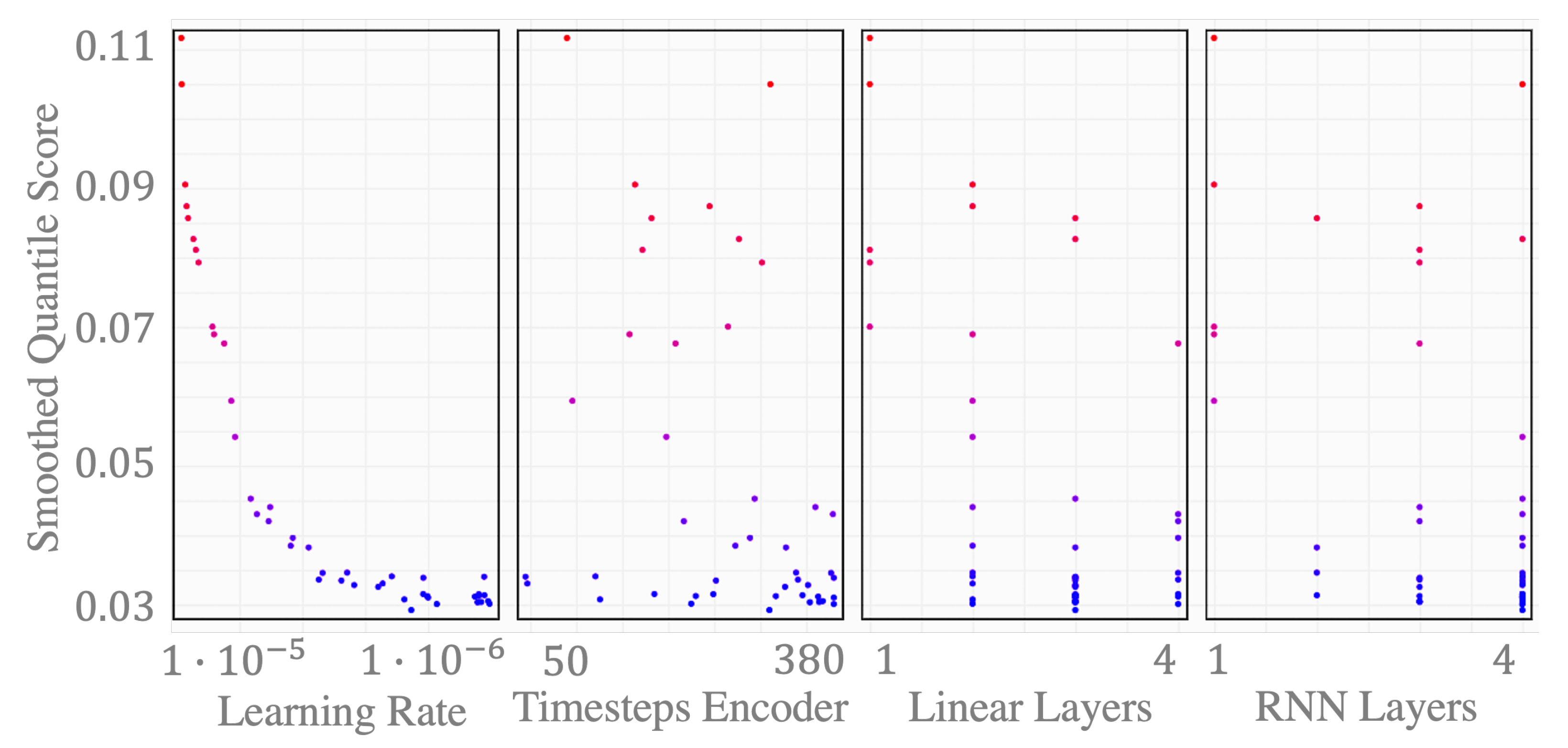
In the scatter plot in Figure 8, we see one marker per hyper parameter trial. The dark blue colors indicate a low score, i.e., the smoothed quantile score , for a PI, as described in Section 2.2.4. We can see that good scores on the validation set can be achieved fairly independently from the history horizon that we chose as the input sequence. With an automatic configuration setting, taking the best parametrization from the hyper parameter optimization study, the history horizon, and thus, length of input sequence to the encoder, is set to 310 steps. The output sequence is always set equal to the forecast horizon, i.e., h, for the day-ahead case. Thirty-eight hours is the time span between the publication of the day-ahead forecasts by the system operators at 10:00 a.m. and the last hour of the following day. With that, inputs that represent future information, such as forecasted wind and PV generation, or dummy variables for future timesteps, are divided into sequences with a length of 38 each.
3.6. Computational Resources
One epoch, given the batch size of 64, takes 2.5 to 5.5 s during training. The training duration is negligible, as it is performed once and does not require re-training, as long as the used training dataset is still representative of the system under study. The machine used for training the models runs with 256 GiB RAM and two Intel Xeon Gold 6128 CPU @ 3.40 GHz. ProLoaF is using the optimized tensor library for deep learning, PyTorch. This framework allows an accelerated tensor computation with GPU. The specification of the CUDA supported GPU that is used in our study is given in Table 5.
3.7. Statistical Evaluation
For the statistical evaluation of the presented forecast models, we apply rolling origin forecasts, i.e., a term introduced by [36], on the test set. The test set is set to 15% of the originally collected data that have not been used during training, validation, and model selection and are thus dedicated to out-of-sample forecasting only.
As we have the actual measurements from the test period, which is from 6 July 2021 to 31 December 2021, we run a day-ahead forecast simulation with a prediction horizon of 38 hourly steps, for each single hour in the test set. One such forecast simulation is referred to as one sample. As we cannot evaluate the accuracy of predicted values, for which the actual measurements lie beyond the test set horizon, we subtract the forecast horizon from the resulting 4277 samples, resulting in 4239 samples. In a next step, we average the metrics, such as RMSE, over the prediction horizon from t = 1 to t = 38 and average these in a next step over all samples. Thus, we obtain the performance metrics presented in Table 6.
We see that Prophet achieves a slightly higher accuracy with a higher forecast skill score of 0.1829 (when using the error metric RMSE) in reference to the auto.arima model. With the tighter prediction interval, which becomes apparent with a smaller sharpness, the certainty of the Prophet forecast is higher than that of the auto.arima model. As a consequence, 12.81% of the actual values do not lie within the simulated prediction intervals. With an overall smaller MIS, we select Prophet as model candidate for the economic benchmark.
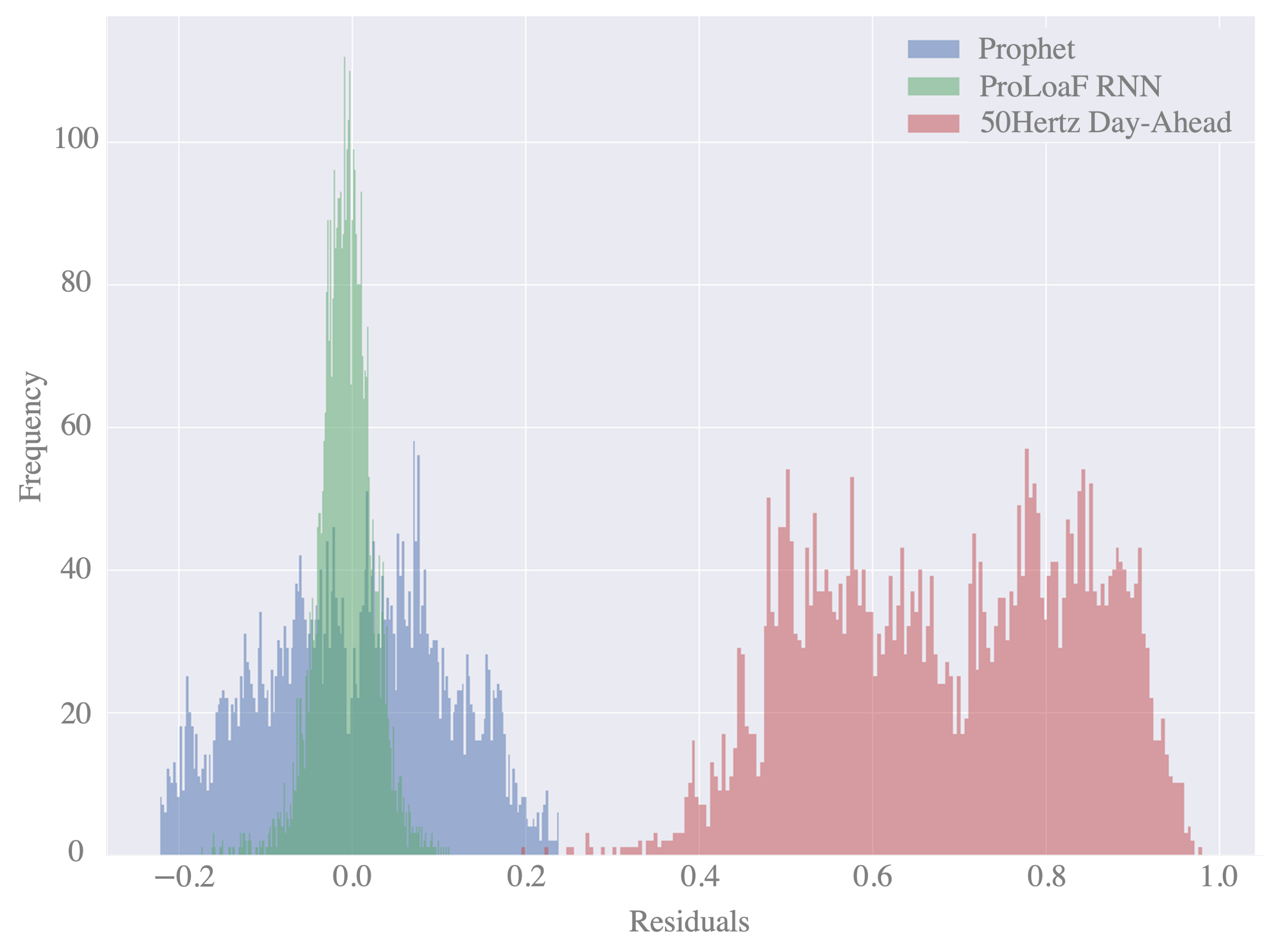
Figure 9 shows the histogram of residuals for the two forecast models. We see a high variance of the residuals in the case of the Prophet forecast but also in the day-ahead forecast values.
Moving on to an economic assessment, as described in Section 3.1, the short-term operational planning context is quite complex and involved multiple physical and non-physical trades of energy or capacity products with or without actual delivery of the product. At the same time, some of the remedial actions are done at zero cost, as they are grid-based measures. A quantification of the forecast value in this context would require a scenario-based market study and simulation, which goes beyond the aim of this work. To be able to still quantify the value of accurate forecasting over the time, we approximate the potential by obtaining the total cost C over all forecast samples, with
for balancing the difference between day-ahead forecast and actual net load, using the day-ahead price for the hour t. Here, m denotes those out-of-sample forecasts that are produced, with a time origin at 10:00 a.m. prior to the delivery day. Thus, the resulting simulation includes 178 full forecast days.
For the difference , we write the absolute difference
Thus, denotes the difference between day-ahead forecast and actual load per timestep and per sample. The day-ahead price in the test period had a mean value of 141.74 €/MWh with a minimum value of −63.03 €/MWh and a maximum value of 442.90 €/MWh.
Table 7 shows the approximate consequence for the case that all forecast errors could be perfectly matched one day prior to the delivery through an hourly energy product, via the day-ahead market. This underlines the importance to have forecasting models that are overall performing more accurately, as the amount of remedial actions needed, given large forecast errors, is increasing significantly. For this, the RMSE is already a qualified indicator.
We further elaborate the effect on one selected snapshot of a holiday week that is typically difficult to forecast with data-driven models, due to a lack of historic data to learn the holiday characteristics. Figure 10 shows the per unit (p.u.) net load in the 2021 winter Christmas holiday week. Here, we highlight two independent sections of the profile in the evening of Monday the 20 of December and in the evening of Christmas Eve on December 24. It is evident that the auto-ML model Prophet is a better candidate to forecast the second segment, whereas ProloaF proves to be better in the first one. In this case, the day-ahead price for the first segment was higher than on Christmas Eve. Because the data point, described in Article 6.1.A, is the basis for the studied data driven models, the predictions inherently learn the impact of the import/export agreements. This explains the offset between the 50 HzT prediction and the two ML models.
4. Discussion
Our analysis shows that the encoder-decoder forecasting model outperforms auto-ML methods on average. As it is trained to produce a symmetric 95% prediction interval, it also produces a zero-mean error on the out-of-sample data. The model was trained with a pre-selection of a parameter search space. The parameters were found using the auto-tuning function implemented with Optuna. Whereas the Auto-ML model Prophet trains much faster (within few seconds), the RNN training requires on average 4 s per epoch. Assuming 50 epochs until one parameter trial is tuned, and 100 trials per training study, the training would take roughly 5 to 6 h on a CUDA supported machine. The study could be designed smaller with fewer trials and fewer epochs with a more advanced pre-selection of the hyperparameters, but the fitting time will remain longer than fitting statistical models such as ARIMA, Prophet, or XGBoost. How many trials are needed to tune the forecast depends on the starting point and the number and value range of potential hyperparameters. The duration of the training time should not be a major concern in today’s operational power system business, as computing resources can be increased flexibly and cost-efficiently, e.g., through cloud computing. Thus, it is rather a question whether a more accurate forecasting model will provide sufficient economic benefit to at least offset the cost of (re)training on dedicated hardware when needed.
Because the prediction time of all models lie within few seconds, they are not benchmarked in detail. Given the critical context of day-ahead operational decisions to counteract unforeseen operation states, a higher accuracy on the whole time series is needed. When forecast models perform equally well, a detailed comparison based on the operational context would need to be considered during deployment and in operation. Although one model may perform the best in general, another model may outperform it in special situations such as holidays.
In the final context, a trade-off study must be conducted for which there is a minimum requirement the forecast model must fulfill, including situations that are critical in a next step from an economic perspective. One solution may be to generate ensemble methods, customized to the specific business needs, which combine the strengths of multiple forecast model candidates.
With this development, more complex models emerge that are less transparent or understandable for the decision makers. However, as described in [37], when forecast models lack interpretability towards particular time series, the trust and confidence of stakeholders can suffer when making decisions. Therefore, we implement an interpretation module in ProLoaF to support the utilization and potential further tuning of the forecast model, with inputs from the operational stage of the MLOps workflow (see Figure 1). Here, MLOps refers to the combination of processes from data preparation, model development and validation to continuous integration and deployment.
4.1. Making a Black-Box Sequence-to-Sequence Model Intepretable
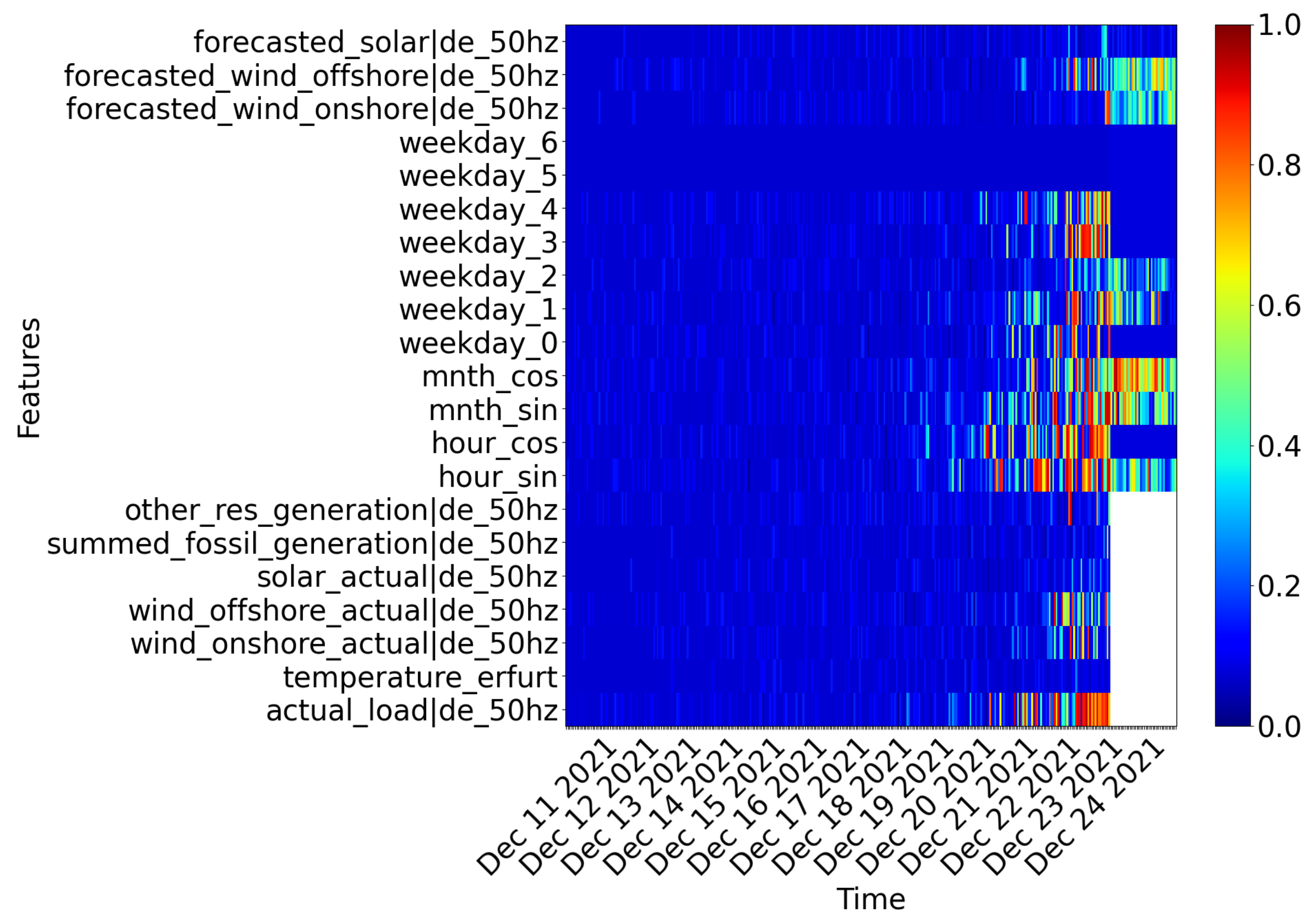
If we want to explore which features the ProLoaF RNN relies on to predict the profile in our case study on Christmas Eve, we can consult saliency maps, as shown in Figure 11.
In essence, a saliency map is a mask matrix with values in the range from 0 to 1. This mask is applied to the data, which we, in the case of the encoder-decoder RNN in Proloaf, split into specific intervals. The time interval comprises the history horizon and the forecasting horizon, which define the encoder and decoder ’length’, respectively. The saliency map corresponds to representation of the encoder-decoder setting in a plane.
The color coding allows one to reflect on the impact of the input features on the prediction target. More specifically, each feature’s importance can change from one time step to another. Whether a feature’s exact value is critical is identified by perturbing each feature value per timestep. A highly perturbated data input has the mask value , indicated in blue. The original input data, with zero perturbation, have the mask value . Following the smallest supporting region principle, we are searching for the smallest element in the input plane that alone is responsible for a high forecast accuracy. To find it, the mask has to be restricted with a constraint in the mask optimization problem formulation. In doing so, only a small region will be achieved that is not perturbed, while keeping the forecast score as high as possible. In that sense, non-perturbed values (shown in red) or slightly perturbed values (yellow to green) indicate that the exact original input data of these features at those timesteps alone would allow a similar prediction compared to the original prediction. The relevant timesteps studied are those of the recent past, corresponding to the input data of encoder features that are shown on the left part of the salience map, up until the forecast window, i.e., 24 December. Here, the decoder features are shown on the right side of the saliency map. All timesteps of input features (both in the encoder and decoder) that have a high mask value, i.e., close to one, are those values that are needed to provide an accurate forecast for the forecast sample under study. As a consequence, we can interpret the red-colored regions of the map as important features.
In [38], the optimization algorithm to generate these maps is proposed as one solution to obtain transparency in deep learning models in a model-agnostic manner. In accordance with the implementation presented in [38], we use Gaussian noise as reference values that disturb our original selected features (here: temperature, wind-offshore, etc.). In a next step, we find the regularization parameter that is set to in this study. All spots in the saliency map that are dark blue can either be largely disturbed or are not beneficial to accurately predict the profile on the example day. Light blue and yellow spots indicate times in which certain features, such as the wind offshore forecasts, are useful but not critical in the sense of their accuracy. The saliency map in Figure 11, for instance, shows on the top right corner for all wind forecast values that are embedded for the prediction horizon in the decoder are disturbed with Gaussian noise, but yet are useful to not further decrease the prediction accuracy. This tells us that the RNN model used needs this information, but the actual precision of the wind generation forecast is less critical. For the dummy cyclical variables of the hour of the day, some weekdays ( = ‘Mondays’) and the recent past information of the actual new load, which we embed in the encoder, the saliency maps reveals a high relevance. As feedback to the forecasting development, one could forward the fact that the weekday features could potentially be re-designed, as 24 December is a Friday, but the future information in the decoder on seems to remain unused. In addition, the input sequence length to the decoder seems to be too long, or at least, the model does not seem to utilize the information that is beyond the last 4–5 days. Furthermore, neither solar forecast nor actual measurement are critical for the selected prediction. As a final remark, the temperature feature is not used in this period, although from a domain knowledge perspective, described in Section 3.2, we assumed that this feature will benefit the model performance.
Thus, we take these insights to design an ablation study in which we remove the blue areas for the encoder size, the temperature feature, the solar features, and the fossil generation feature.
4.2. Ablation Study
In the ablation study, we compare the earlier presented ProLoaF RNN with new trained versions with slightly modified configurations. Each ablation is an isolated study. We do not aggregate the modification, so that, the “-no PV”-configuration still includes a history horizon of 310 h.
The study results in Table 8 show that the forecast model is robust with regard to slightly different configurations. Only one modification could be considered as a better candidate for deployment, i.e., the configuration with no temperature feature, in the model development stage. Alternatively, the temperature measurement could be re-addressed in the EDA stage.
4.3. Designing MLOps
In recent years, the need for forecasting in power system operations has increased. With that need, tools have been deployed to solve the forecasting problem, but also to make these new data streams available in the control room. The focus in ProLoaF was the development of a robust, reliable, data-driven probabilistic forecast model. As ProLoaF is an integrated worker in SOGNO, the project aims to be an exploitable contribution to MLOps for forecasting in the power system control room. In addition to ProLoaF, Linux Foundation Energy also hosts an open source project forecasting project, OpenSTEF [39], which has a stronger focus on the deployment, sanity checks, and re-calibration of forecasting models in the control room. The projects are compatible, in the sense that ProLoaF is applicable as regressor object in OpenSTEF and is openly available for utilization and contribution by the forecasting and power system community.
5. Conclusions
The forecast evaluation based on established forecast error statistics on one side, and the economic valuation of the applied forecast on the other side, was conducted on out-of-sample predictions for the period from July to December 2021. The discussion shows that besides mere forecast evaluation on the average performance of the time series prediction, a thorough analysis of the error variation over time is particularly interesting. The trade-off during model tuning and development depends very much on the decision making context.
An encoder-decoder RNN model was designed to predict the net load under uncertainty and was found to outperform the multivariate auto.arima method and the uni-variate Prophet method, which were promising auto-ML candidates for the described case study.
It was further determined that ML models in critical operational contexts necessitate tools that accompany the model to increase transparency. With a better understanding of the prediction logic, not only the trust on the operator’s end can be increased but also more precise insights can be fed back to the preparatory development stages of the ML pipeline. With the presented generic framework of ProLoaF, the deep learning forecasting core can be extended with further encoder-decoder type of neural network architectures. Recent advances on statistical models, such as ETSarima or FFORMA, which are currently leading the time series competitions (M4 and M5 [14,40]), could be studied and benchmarked with new advances from the deep learning community. Here, specifically, temporal fusion transformer models [41] are potential candidates to extend the presented study in the future.
Author Contributions
Conceptualization, methodology, software, validation, formal analysis, investigation, resources, data curation, writing—original draft preparation, visualization, editing, project administration, G.G.-T.; writing—review and supervision, G.G.-T. and A.M.; funding acquisition, A.M. All authors have read and agreed to the published version of the manuscript.
Funding
This research was funded by European Union’s Horizon 2020 research and innovation programme under Grant Agreement No. 824414 https://coordinet-project.eu/ (accessed on 4 April 2022).
Institutional Review Board Statement
Not applicable.
Informed Consent Statement
Not applicable.
Data Availability Statement
Power system data sources openly available at https://transparency.entsoe.eu (accessed on 25 May 2022). Meteorological data sources openly available at https://www.dwd.de/ (accessed on 25 May 2022). Algorithm openly available at https://github.com/sogno-platform/proloaf (accessed on 25 May 2022).
Acknowledgments
The authors gratefully acknowledge E.ON Energidistribution for providing the initial forecasting problem formulation and requirements for the demonstration in the H2020 CoordiNet project. The authors also acknowledge the collaboration with Alliander N.V. within Linux Foundation Energy to implement ProLoaF as deep learning module in the open machine learning energy forecasting pipeline OpenSTEF. This study has made use of recent historical meteorological data provided by DWD (Deutscher Wetterdienst, https://www.dwd.de/) (accessed on 25 May 2022).
Conflicts of Interest
The authors declare no conflict of interest.
Abbreviations
The following abbreviations are used in this manuscript:
| ADAM | Adaptive Moment Estimation |
| AIC | Akaike’s Information Criterion |
| ANN | Artificial Neural Network |
| ARIMA | Autoregressive Integrated Moving Average |
| ASM | Active Power System Management |
| CDF | Cumulative Distribution Function |
| CPU | Central Processing Unit |
| CUDA | Compute Unified Device Architecture |
| DSO | Distribution System Operator |
| DWD | Deutscher Wetterdienst |
| EDA | Explorative Data Analysis |
| GAMs | General Additive Methods |
| GPU | Graphics Processing Unit |
| GRU | Gated Recurrent Unit |
| LSTM | Long-Short-Term Memory Units |
| MASE | Mean Absolute Scaled Error |
| MIS | Mean Interval Score |
| ML | Machine Learning |
| MLOps | Machine Learning Operations |
| MSE | Mean Squared Error |
| PI | Prediction Interval |
| PICP | Prediction Interval Coverage Probability |
| PLF | Probabilistic Load Forecasting |
| PV | Photovoltaics |
| QRF | Quantile Regression Forests |
| QS | Quantile Score |
| RES | Renewable Energy Source |
| RMSE | Root Mean Squared Error |
| RNN | Recurrent Neural Network |
| Seq2Seq | Sequence to Sequence Learning Neural Networks |
| SOGNO | Service-based Open-source Grid Automation Platform for Network Operation of the Future |
| STLF | Short Term Load Forecasting |
| TPE | Tree-Structured Parzen Estimator |
| TSO | Transmission System Operator |
| XGBoost | Extreme Gradient Boosting |
References
- CEDEC; E.DSO; ENTSO-E; EURELECTRIC; GEODE (Eds.) TSO–DSO Report: An Integrated Approach to Active System Management; CEDEC; E.DSO; ENTSO-E; EURELECTRIC; GEODE: Brussels, Belgium, April 2019. [Google Scholar]
- Kloubert, M.L.; Schwippe, J.; Muller, S.C.; Rehtanz, C. Analyzing the impact of forecasting errors on redispatch and control reserve activation in congested transmission networks. In Proceedings of the 2015 IEEE Eindhoven PowerTech, Eindhoven, The Netherlands, 29 June–2 July 2015; pp. 1–6. [Google Scholar]
- Gürses-Tran, G. ProLoaF: V0.2.2. 2021. Available online: https://zenodo.org/record/6408478#.Yo8y4VRBxPY (accessed on 25 May 2022).
- Messner, J.W.; Pinson, P.; Browell, J.; Bjerregård, M.B.; Schicker, I. Evaluation of wind power forecasts—An up-to-date view. Wind. Energy 2020, 23, 1461–1481. [Google Scholar] [CrossRef] [Green Version]
- Hyndman, R.J.; Athanasopoulos, G. (Eds.) Forecasting: Principles and Practice; Otexts: Lexington, Kentucky, May 2018. [Google Scholar]
- Dobschinski, J.; Bessa, R.; Du, P.; Geisler, K.; Haupt, S.E.; Lange, M.; Möhrlen, C.; Nakafuji, D.; de la Torre Rodriguez, M. Uncertainty Forecasting in a Nutshell: Prediction Models Designed to Prevent Significant Errors. IEEE Power Energy Mag. 2017, 15, 40–49. [Google Scholar] [CrossRef] [Green Version]
- Hong, T.; Pinson, P.; Wang, Y.; Weron, R.; Yang, D.; Zareipour, H. Energy Forecasting: A Review and Outlook. IEEE Open Access J. Power Energy 2020, 7, 376–388. [Google Scholar] [CrossRef]
- Murphy, A.H. What Is a Good Forecast? An Essay on the Nature of Goodness in Weather Forecasting. Weather. Forecast. 1993, 8, 281–293. [Google Scholar] [CrossRef] [Green Version]
- Bessa, R.J.; Miranda, V.; Botterud, A.; Wang, J. ‘Good’ or ‘bad’ wind power forecasts: A relative concept. Wind. Energy 2011, 14, 625–636. [Google Scholar] [CrossRef]
- Haupt, S.E.; Casado, M.G.; Davidson, M.; Dobschinski, J.; Du, P.; Lange, M.; Miller, T.; Mohrlen, C.; Motley, A.; Pestana, R.; et al. The Use of Probabilistic Forecasts: Applying Them in Theory and Practice. IEEE Power Energy Mag. 2019, 17, 46–57. [Google Scholar] [CrossRef]
- Bracale, A.; Caramia, P.; Falco, P.D.; Hong, T. Multivariate Quantile Regression for Short-Term Probabilistic Load Forecasting. IEEE Trans. Power Syst. 2020, 35, 628–638. [Google Scholar] [CrossRef]
- Toubeau, J.F.; Bottieau, J.; Vallee, F.; de Greve, Z. Deep Learning-Based Multivariate Probabilistic Forecasting for Short-Term Scheduling in Power Markets. IEEE Trans. Power Syst. 2019, 34, 1203–1215. [Google Scholar] [CrossRef]
- Makridakis, S.; Spiliotis, E.; Assimakopoulos, V. The M4 Competition: 100,000 time series and 61 forecasting methods. Int. J. Forecast. 2020, 36, 54–74. [Google Scholar] [CrossRef]
- Makridakis, S.; Spiliotis, E.; Assimakopoulos, V. M5 accuracy competition: Results, findings, and conclusions. Int. J. Forecast. 2022, 36, 224–227. [Google Scholar] [CrossRef]
- Farrokhabadi, M.; Browell, J.; Wang, Y.; Makonin, S.; Su, W.; Zareipour, H. Day-Ahead Electricity Demand Forecasting Competition: Post-COVID Paradigm. IEEE Open Access J. Power Energy 2022, 1. [Google Scholar] [CrossRef]
- Gürses-Tran, G.; Flamme, H.; Monti, A. Probabilistic Load Forecasting for Day-Ahead Congestion Mitigation. In Proceedings of the 16th International Conference on Probabilistic Methods Applied to Power Systems, PMAPS 2020, Liege, Belgium, 18–21 August 2020; pp. 1–6. [Google Scholar]
- Sutskever, I.; Vinyals, O.; Le, V.Q. Sequence to Sequence Learning with Neural Networks. Adv. Neural Inf. Process. Syst. 2014, 27, 5–8. [Google Scholar]
- Bottieau, J.; Hubert, L.; De Greve, Z.; Vallee, F.; Toubeau, J.F. Very-Short-Term Probabilistic Forecasting for a Risk-Aware Participation in the Single Price Imbalance Settlement. IEEE Trans. Power Syst. 2020, 35, 1218–1230. [Google Scholar] [CrossRef]
- Friedman, J.H. Greedy function approximation: A gradient boosting machine. Ann. Stat. 2001, 29, 1189–1232. [Google Scholar] [CrossRef]
- Seabold, S.; Perktold, J. statsmodels: Econometric and statistical modeling with python. In Proceedings of the 9th Python in Science Conference, Austin, TX, USA, 28 June–3 July 2010. [Google Scholar]
- Taylor, S.J.; Letham, B. Forecasting at Scale. Am. Stat. 2018, 72, 37–45. [Google Scholar] [CrossRef]
- Gneiting, T.; Balabdaoui, F.; Raftery, A.E. Probabilistic forecasts, calibration and sharpness. J. R. Stat. Soc. Ser. 2007, 69, 243–268. [Google Scholar] [CrossRef] [Green Version]
- Gneiting, T.; Raftery, A.E. Strictly Proper Scoring Rules, Prediction, and Estimation. J. Am. Stat. Assoc. 2007, 102, 359–378. [Google Scholar] [CrossRef]
- Hyndman, R.J.; Koehler, A.B. Another look at measures of forecast accuracy. Int. J. Forecast. 2006, 22, 679–688. [Google Scholar] [CrossRef] [Green Version]
- Petropoulos, F.; Apiletti, D.; Assimakopoulos, V.; Babai, M.Z.; Barrow, D.K.; Taieb, S.B.; Bergmeir, C.; Bessa, R.J.; Bijak, J.; Boylan, J.E.; et al. Forecasting: Theory and practice. arXiv 2020, arXiv:2012.03854. [Google Scholar] [CrossRef]
- Barandas, M.; Folgado, D.; Fernandes, L.; Santos, S.; Abreu, M.; Bota, P.; Liu, H.; Schultz, T.; Gamboa, H. TSFEL: Time Series Feature Extraction Library. SoftwareX 2020, 11, 100456. [Google Scholar] [CrossRef]
- Taylor, G.S. pmdarima: ARIMA Estimators for Python. 2017. Available online: http://www.alkaline-ml.com/pmdarima (accessed on 25 May 2022).
- Rimi, N.F.; Bast, H.; Wittwer, C. Comparative Study of Forecasting Algorithms for Energy Data. 2019. Available online: https://ad-publications.informatik.uni-freiburg.de/theses/Master_Nishat_Fariha_Rimi_2019.pdf (accessed on 25 May 2022).
- Akiba, T.; Sano, S.; Yanase, T.; Ohta, T.; Koyama, M. Optuna: A Next-generation Hyperparameter Optimization Framework. In Proceedings of the 25rd ACM SIGKDD International Conference on Knowledge Discovery and Data Mining, Anchorage, AK, USA, 4–8 August 2019. [Google Scholar]
- Ashour Novirdoust, A.; Bichler, M.; Bojung, C.; Buhl, H.; Fridgen, G.; Gretschko, V.; Hanny, L.; Knörr, J.; Maldonado, F.; Neuhoff, K.; et al. Electricity Sport Market Design 2030–2050. In Report, Fraunhofer-Publica; The Institute of Energy Economics at the University of Cologne (EWI): Cologne, Germany, 2021. [Google Scholar] [CrossRef]
- Val Leeuwen, T.; Meinerzhagen, A.K.; Raths, S.; Roether, A. Integration kurativer Maßnahmen in das Engpassmanagement im deutschen Übertragungsnetz. In Symposium Energieinnovation; Amprion: Graz, Austria, 2020. [Google Scholar]
- 50Hertz Transmission GmbH. Daten und Fakten 2019; 50Hertz Transmission GmbH: Berlin, Germany, 2020; Available online: https://www.50hertz.com (accessed on 25 May 2022).
- Böttcher, F.; Deutschländer, T.; Friedrich, A.; Friedrich, K.; Fröhlich, K.; Früh, B.; Ganske, A.; Heinrich, H.; Kreienkamp, F.; Malitz, G.; et al. National Climate Report. In Report, Deutscher Wetterdienst; Deutscher Wetterdienst: Offenbach am Main, Germany, 2017. [Google Scholar]
- Kingma, D.P.; Ba, J. Adam: A Method for Stochastic Optimization. In Proceedings of the 3rd International Conference on Learning Representations, ICLR 2015, San Diego, CA, USA, 7–9 May 2015. [Google Scholar]
- NVIDIA. NVIDIA Data Center Inference Products: Performance Specs. 2022. Available online: https://www.nvidia.com/en-us/deep-learning-ai/solutions/inference-platform/hpc/ (accessed on 25 May 2022).
- Tashman, L.J. Out-of-sample tests of forecasting accuracy: An analysis and review. Int. J. Forecast. 2000, 16, 437–450. [Google Scholar] [CrossRef]
- Rajapaksha, D.; Bergmeir, C.; Hyndman, R.J. LoMEF: A Framework to Produce Local Explanations for Global Model Time Series Forecasts. arXiv 2021, arXiv:2111.07001. [Google Scholar]
- Gürses-Tran, G.; Körner, T.A.; Monti, A. Introducing Explainability in Sequence-to-Sequence Learning for Short-term Load Forecasting. Electr. Power Syst. Res. 2022, in press. [Google Scholar]
- Alliander N.V. OpenSTEF–Automated Machine Learning Pipelines. In Builds the Open Short Term Forecasting Package; Alliander N.V.: Arnhem, The Netherlands, 2022. [Google Scholar]
- Makridakis, S.; Hyndman, R.J.; Petropoulos, F. Forecasting in social settings: The state of the art. Int. J. Forecast. 2020, 36, 15–28. [Google Scholar] [CrossRef]
- Lim, B.; Arık, S.O.; Loeff, N.; Pfister, T. Temporal Fusion Transformers for interpretable multi-horizon time series forecasting. Int. J. Forecast. 2021, 37, 1748–1764. [Google Scholar] [CrossRef]
Figure 1.
MLOps workflow.

Figure 2.
Exemplary unfolded encoder-decoder architecture of sequence-to-sequence RNN. We pass inputs on both the encoder and decoder sides. The number of the layer stack is subject to parameterization. The gray boxes represent RNN cells.
Figure 2.
Exemplary unfolded encoder-decoder architecture of sequence-to-sequence RNN. We pass inputs on both the encoder and decoder sides. The number of the layer stack is subject to parameterization. The gray boxes represent RNN cells.

Figure 3.
Timeline of the consecutive operational planning processes of the German transmission system operators. Graphical representation adapted from [31].
Figure 3.
Timeline of the consecutive operational planning processes of the German transmission system operators. Graphical representation adapted from [31].

Figure 4.
Figures of generation, load, and import-exports in 50 HzT Zone (Year 2019). Data source: Entsoe Transparency Platform [32].
Figure 4.
Figures of generation, load, and import-exports in 50 HzT Zone (Year 2019). Data source: Entsoe Transparency Platform [32].

Figure 5.
Average net load profiles per season from October 2018 to December 2021. See: Entsoe Transparency Platform [32].
Figure 5.
Average net load profiles per season from October 2018 to December 2021. See: Entsoe Transparency Platform [32].

Figure 6.
Cost for redispatch measures in the 50 HzT grid since 2017, varying over the time of the year.
Figure 6.
Cost for redispatch measures in the 50 HzT grid since 2017, varying over the time of the year.

Figure 7.
Cost for redispatch measures in the 50 HzT since 2017, varying over the time of the year.

Figure 8.
Scatter plot of optimal hyperparameter search.

Figure 9.
Histogram of residuals.

Figure 10.
Comparison of forecast profiles with actual load in winter week 2021 with Christmas holidays as of 24 December.
Figure 10.
Comparison of forecast profiles with actual load in winter week 2021 with Christmas holidays as of 24 December.

Figure 11.
Saliency map of the feature importance for the prediction on 24 December 2021.


Table 1.
Actual hourly measurement data in MW from 1 October 2018 to 31 December 2021.
| PV | Offshore | Onshore | Other RES | Fossil | Load | |
|---|---|---|---|---|---|---|
| Mean | 1331 | 451 | 3909 | 893 | 8474 | 11,904 |
| Std. Dev. | 2143 | 352 | 3397 | 641 | 2296 | 1977 |
| q(25%) | 0 | 120 | 1258 | 511 | 6878 | 10,973 |
| q(75%) | 1972 | 787 | 5624 | 1056 | 10,136 | 13,359 |
Table 2.
Hourly forecast data in MW from 1 October 2018 to 31 December 2021.
| PV | Offshore | Onshore | Load | |
|---|---|---|---|---|
| Mean | 1327 | 467 | 3930 | 10,397 |
| Std. Dev. | 2110 | 345 | 3322 | 1816 |
| q(25%) | 0 | 142 | 1357 | 8992 |
| q(75%) | 1990 | 794 | 5541 | 12,008 |
Table 3.
Fitting ARIMA models.
| ARIMA | ARIMAX | SARIMA | SARIMAX | |
|---|---|---|---|---|
| Season | - | - | 24 | 24 |
| Exog. | None | Temperature Wind Onshore Wind Offshore PV Conventional Other RES | None | Temperature Wind Onshore Wind Offshore PV Conventional Other RES |
| Lag | 168 | 168 | 168 | 168 |
| Model | (2,1,1)(0,0,0)[0] | (2,1,1)(0,0,0)[0] | (1,1,0)(1,0,2)[24] | (4,1,1)(2,0,2)[24] |
| AIC | −9150.47 | −9152.59 | −10,411.57 | −10,570.10 |
Table 4.
Hyper parameter search space for net load forecast with ProLoaF.
| Parameter | Min | Max | Best ProLoaF RNN |
|---|---|---|---|
| Learning Rate | 1 × 10 | 1 × 10 | 7.47 × 10 |
| Batch Size | 32 | 128 | 64 |
| Linear Layers | 1 | 4 | 3 |
| RNN Layers | 1 | 4 | 4 |
Table 5.
GPU performance data (see [35]).
Table 5.
GPU performance data (see [35]).
| Data Points | Tesla P40 |
|---|---|
| Single-Precision Performance (FP32) | 12 TFLOPS |
| Integer Operations (INT8) | 47 TOPS |
| GPU Memory | 24GB |
| Memory Bandwidth | 346 GB/s |
| Power | 250 W |
Table 6.
Average probabilistic forecast performance of the auto.arima, Prophet, and ProLoaF, based on scaled values.
Table 6.
Average probabilistic forecast performance of the auto.arima, Prophet, and ProLoaF, based on scaled values.
| Metric | auto.arima | Prophet | ProLoaF |
|---|---|---|---|
| RMSE | 0.1047 | 0.0696 | 0.0514 |
| Sharpness | 0.4730 | 0.2156 | 0.1748 |
| PICP | 95.88% | 87.19% | 92.17% |
| MIS | 0.5370 | 0.3299 | 0.075 |
Table 7.
Comparison of flat total cost for forecast errors.
| Prophet | ProLoaF | |
|---|---|---|
| Average in MWh | 907.18 | 666.26 |
| Summed in GWh | 3049.95 | 2437.19 |
| Total Cost C in Mio.€ | 580.96 | 352.72 |
Table 8.
Ablation results of presented ProLoaF RNN configuration. The underlined values indicate the best model in the analyzed metric category.
Table 8.
Ablation results of presented ProLoaF RNN configuration. The underlined values indicate the best model in the analyzed metric category.
| Metric | ProLoaF RNN | -No Temp. | -No PV | -No Fossil | Enc. Size (24 h × 6 Days = 144 Time Steps Embedded as Encoder Input Size during Training.) |
|---|---|---|---|---|---|
| MSE | 0.002 | 0.002 | 0.003 | 0.002 | 0.002 |
| RMSE | 0.050 | 0.049 | 0.058 | 0.049 | 0.050 |
| Sharpness | 0.197 | 0.220 | 0.185 | 0.219 | 0.202 |
| PICP | 94.63% | 96.92% | 90.19% | 96.86% | 95.36% |
| RAE | 0.235 | 0.228 | 0.272 | 0.231 | 0.237 |
| MAE | 0.038 | 0.037 | 0.044 | 0.037 | 0.038 |
| MIS | 0.075 | 0.073 | 0.087 | 0.073 | 0.075 |
| MASE | 0.960 | 0.933 | 1.116 | 0.944 | 0.973 |
| QS | 0.025 | 0.025 | 0.030 | 0.024 | 0.025 |
| Residuals | 0.002 | 0.005 | 0.019 | 0.010 | 0.009 |
Publisher’s Note: MDPI stays neutral with regard to jurisdictional claims in published maps and institutional affiliations. |
© 2022 by the authors. Licensee MDPI, Basel, Switzerland. This article is an open access article distributed under the terms and conditions of the Creative Commons Attribution (CC BY) license (https://creativecommons.org/licenses/by/4.0/).
Share and Cite
MDPI and ACS Style
Gürses-Tran, G.; Monti, A. Advances in Time Series Forecasting Development for Power Systems’ Operation with MLOps. Forecasting 2022, 4, 501-524. https://0-doi-org.brum.beds.ac.uk/10.3390/forecast4020028
AMA Style
Gürses-Tran G, Monti A. Advances in Time Series Forecasting Development for Power Systems’ Operation with MLOps. Forecasting. 2022; 4(2):501-524. https://0-doi-org.brum.beds.ac.uk/10.3390/forecast4020028
Chicago/Turabian StyleGürses-Tran, Gonca, and Antonello Monti. 2022. "Advances in Time Series Forecasting Development for Power Systems’ Operation with MLOps" Forecasting 4, no. 2: 501-524. https://0-doi-org.brum.beds.ac.uk/10.3390/forecast4020028