Aesthetical Issues of Leonardo Da Vinci’s and Pablo Picasso’s Paintings with Stochastic Evaluation


Laboratory of Hydrology and Water Resources Development, School of Civil Engineering, National Technical University of Athens, Heroon Polytechneiou 9, 157 80 Zographou, Greece
*
Author to whom correspondence should be addressed.
Heritage 2020, 3(2), 283-305; https://0-doi-org.brum.beds.ac.uk/10.3390/heritage3020017
Submission received: 7 April 2020
/
Revised: 20 April 2020
/
Accepted: 21 April 2020
/
Published: 25 April 2020
(This article belongs to the Section Artistic Heritage)
Abstract
:A physical process is characterized as complex when it is difficult to analyze or explain in a simple way. The complexity within an art painting is expected to be high, possibly comparable to that of nature. Therefore, constructions of artists (e.g., paintings, music, literature, etc.) are expected to be also of high complexity since they are produced by numerous human (e.g., logic, instinct, emotions, etc.) and non-human (e.g., quality of paints, paper, tools, etc.) processes interacting with each other in a complex manner. The result of the interaction among various processes is not a white-noise behavior, but one where clusters of high or low values of quantified attributes appear in a non-predictive manner, thus highly increasing the uncertainty and the variability. In this work, we analyze stochastic patterns in terms of the dependence structure of art paintings of Da Vinci and Picasso with a stochastic 2D tool and investigate the similarities or differences among the artworks.
1. Introduction
The meaning of beauty is linked to the evolution of human civilization, and the analysis of the connection between the observer and the beauty in art and nature has always been of high interest in both philosophy and science. Even though this analysis has mostly been regarded as part of social studies and humanities, other scientists have also been involved mostly through the philosophy of science [1]. Analyses through mathematics are generally focused on applying mathematical tools in trying to describe aesthetics. In most of these analyses, the question at hand is whether what is pleasing to the eye can be explained through analogies.
The word canon, or set of proportions, comes from Greek (κανών) and means a straight rod (measuring line) and, metaphorically, a rule or standard. Canons have changed through history according to artistic needs, taste, and sense of beauty. Pythagoras and Euclid were the first philosophers known to have searched for a common rule (canon) existing in shapes that are perceived as beautiful. Euclid’s Elements (c. 300 BC), notably, includes the first known definition of the golden ratio.
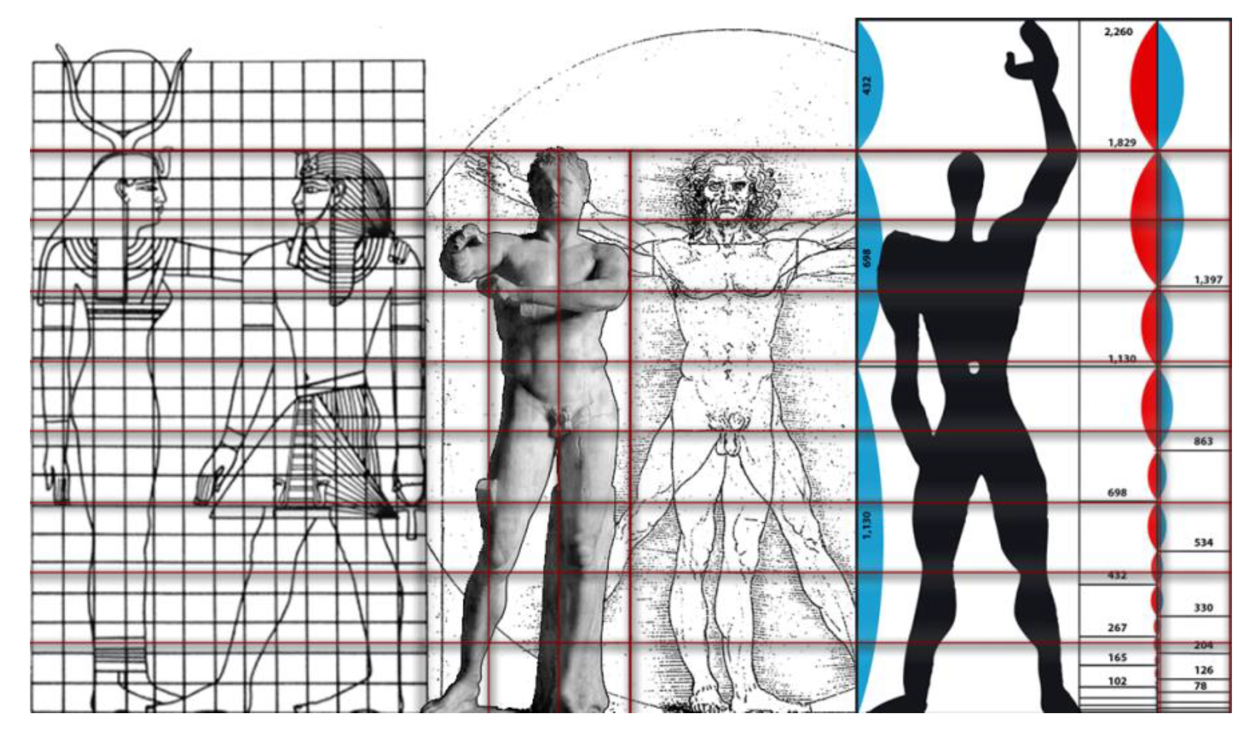
There is an eternal discussion of mathematical canons of proportion as models of beauty for the human body: ancient Egyptian civilization; ancient Greece (Lysippos, Polykleitos); ancient Rome (Vitruvius); Renaissance (Leonardo Da Vinci, Albrecht Dürer); modern times (Adolf Zeising, David Hay, John Pennethorne, Mathieu Lauweriks, Jay Hambidge, Matila Ghyka and Le Corbusier) (Figure 1) [2,3,4,5,6,7].
The opinions of later philosophers on this pursuit of mathematicians for the analysis of aesthetics were more varied. Leibniz, for example, believed that there is a norm behind every aesthetic feeling which we simply do not know how to measure [8]. On the contrary, Descartes supports that instead of regarding the aesthetic quality as an inherent property of a physical object, the distinction of mind and nature has allowed humans to incorporate their own subjective emotional, social and cognitive background in determining their aesthetic preferences. Overall, it is evident that many artists knew and applied math and geometry in their artwork (Figure 2) and many philosophers tried to connect math and arts. [9,10,11]
New researchers are trying to create art using computational intelligence technologies. In particular, evolutionary computation has been able to generate visual art and music [12,13,14,15]. Evaluation of the items generated by evolutionary algorithms is a key issue in computational creativity. Experimental results show that artificial intelligence technologies can generate satisfactory paintings by using some kind of aesthetic evaluation [6,7,8,9,10,11,12,13,14,15,16,17].
Mathematics has been part of the art, but can it be used in evaluating the art? The evaluation of art paintings [18,19,20,21,22,23,24,25,26] is a difficult and subjective process and in order to create an objective process, image evaluation and classification of art paintings with mathematical algorithms is the subject of a plethora of related publications [27,28,29,30,31,32,33,34,35,36,37,38,39,40,41,42,43,44,45,46,47,48,49,50,51,52,53,54,55,56,57,58,59,60,61,62].
The mathematical field of Stochastics has been introduced as an alternative to deterministic approaches, to model the so-called random (i.e., complex, unexplained or unpredictable) fluctuations observed in non-linear geophysical processes [63,64]. Stochastics helps develop a unified perception for natural phenomena and expel dichotomies like random vs. deterministic. Particularly, there is no such thing as a ‘virus of randomness’ that infects some phenomena to make them random, leaving other phenomena uninfected. It seems, rather, that both randomness and predictability coexist and are intrinsic to natural systems which can be deterministic and random at the same time, depending on the prediction horizon and the time scale [65]. On this basis, the uncertainty in art, as in other processes of nature, can be both aleatory (alea = dice) and epistemic (as, in principle, we could know perfectly the underlying mechanisms). Therefore, dichotomies such as ‘deterministic vs. random’ and ‘aleatory vs. epistemic’ may be false ones and may lead to paradoxes. By applying the concept of stochastic analysis, we can identify the observed unpredictable fluctuations of systems under investigation with the variability of a devised stochastic process.
2. Methodology
2.1. Stochastic Analysis in 2D
In this research paper, a stochastic computational tool called 2D-C [66] is used to analyze art paintings in order to: (a) examine stochastic similarities and differences among artworks; (b) introduce a methodology for evaluating restoration aspects with stochastic tools; (c) identify the stochastic meaning of specific areas of the artworks; and (d) examine the originality of art paintings (or parts of art paintings) with stochastic tools.
2D-C measures the degree of variability (change in variability vs. scale) in images using stochastic analysis. Apparently, beauty is not easy to quantify with stochastic measures, but nevertheless the examination of artworks through a stochastic analysis offers interesting insights into aspects of the art paintings. The stochastic analyses of the examined artworks are presented using climacograms based on the 2D-C analysis of image pixels.
Image processing typically involves filtering or enhancing an image using various types of functions, in addition to other techniques, to extract information from the images [67]. Image segmentation is one of the basic problems in image analysis. The importance and utility of image segmentation has resulted in extensive research and numerous proposed approaches based on intensity, color, texture, etc., and both automatic and interactive [68]. A variety of techniques have been proposed for the quantitative evaluation of segmentation methods [69,70,71,72,73,74,75,76].
This analysis for image processing is based on a stochastic tool called a climacogram. The term climacogram [77,78] comes from the Greek word climax (meaning scale). It is defined as the (plot of) variance of the averaged process (assuming it is stationary) versus averaging time scale k, and is denoted as γ(k). The climacogram is useful for detecting the long-term change (or else dependence, persistence or clustering) of a process, which emerges particularly in complex systems, as opposed to white-noise (absence of dependence) of even Markov (i.e., short-term persistence) behavior [79].
In order to obtain data for the evaluation of art paintings, each image of art painting is digitized in 2D based on a grayscale color intensity (thus this climacogram studies the brightness of an image), and the climacogram is calculated based on the geometric scales of adjacent pixels. Assuming that our sample is an area nΔ × nΔ, where n is the number of intervals (e.g., pixels) along each spatial direction, and Δ is the discretization unit (determined by the image resolution, e.g., pixel length), the empirical classical estimator of the climacogram for a 2D process can be expressed as:
where the ‘^’ over γ denotes estimate, is the the dimensionless spatial scale, is the sample average of the space-averaged process at scale , and is the sample average. Note that the maximum available scale for this estimator is n/2. The difference between the value in each element and the field mean is raised to the power of 2, since we are mostly interested in the magnitude of the difference rather than its sign. Thus, the climacogram expresses in each scale the diversity in the brightness among the different elements. In this manner, we may quantify the uncertainty of the brightness intensities at each scale by measuring their variability.
In order to characterize stochastic analysis of the data, an important property is the Hurst–Kolmogorov (HK) behavior (usually known in hydrometeorological processes as Long Term Persistence, or LTP), which can be summarized by the Hurst parameter as follows. The isotropic HK process with an arbitrary marginal distribution (e.g., for the Gaussian one, this results in the well-known fractional-Gaussian-noise, described by Mandelbrot and van Ness [80]), i.e., the power-law decay of variance as a function of scale, is defined for a 1D or 2D process as:
where is the variance at scale k = κΔ, d is the dimension of the process/field (i.e., for a 1D process d = 1, for a 2D field d = 2, etc.), and H is the Hurst parameter (0 < H < 1). For 0 < H < 0.5 the HK process exhibits an anti-persistent behavior, H = 0.5 corresponds to the white noise process, and for 0.5 < H < 1 the process exhibits LTP (clustering). In the case of clustering behavior due to the non-uniform heterogeneity of the brightness of the painting, the high variability of the brightness persists even in large scales. This clustering effect may greatly increase the diversity between the brightness in each pixel of the image, a phenomenon also observed in hydrometeorological processes (such as temperature, precipitation, wind, etc.), natural landscapes [66] and music [81]. Therefore, it is interesting to observe the degrees of uncertainty and variability in arts.
The algorithm that generates the climacogram in 2D was developed in MATLAB for rectangular images [82]. In particular, for the current analysis, the images are cropped to 400 × 400 pixels, 14.11 cm × 14.11 cm, in 72 dpi (dots per inch).
2.2. Illustration of Stochastic Analysis in 2D
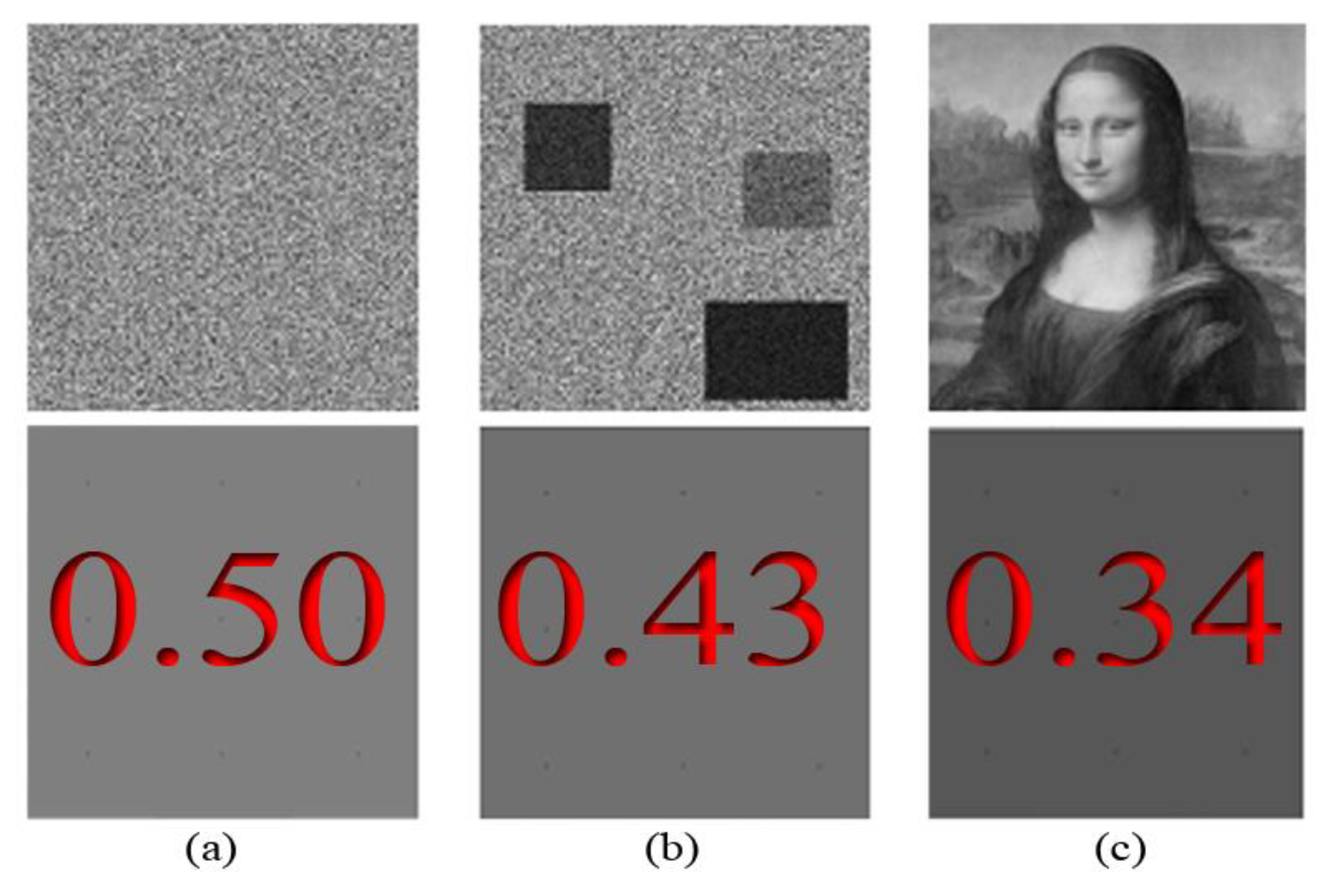
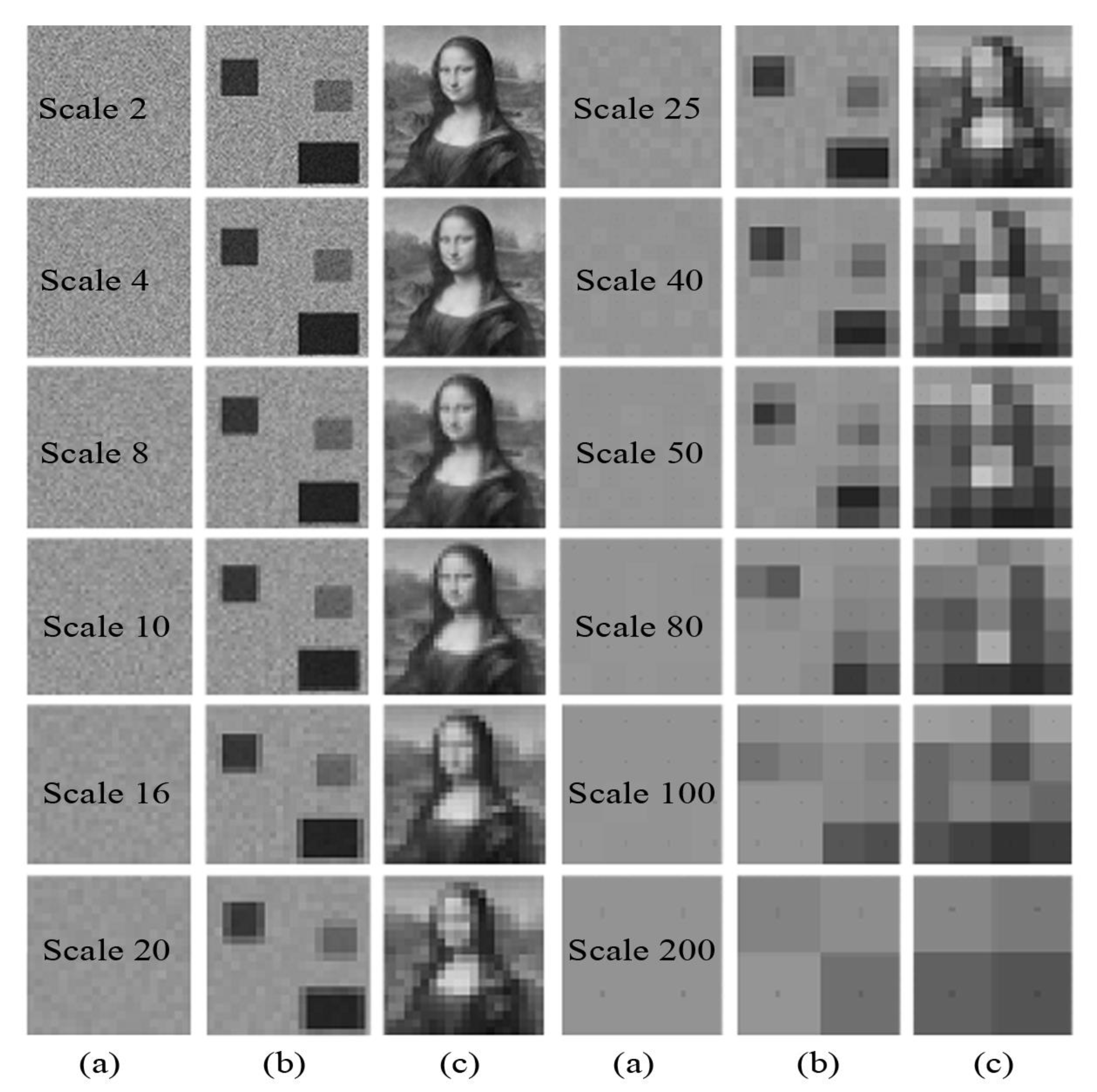
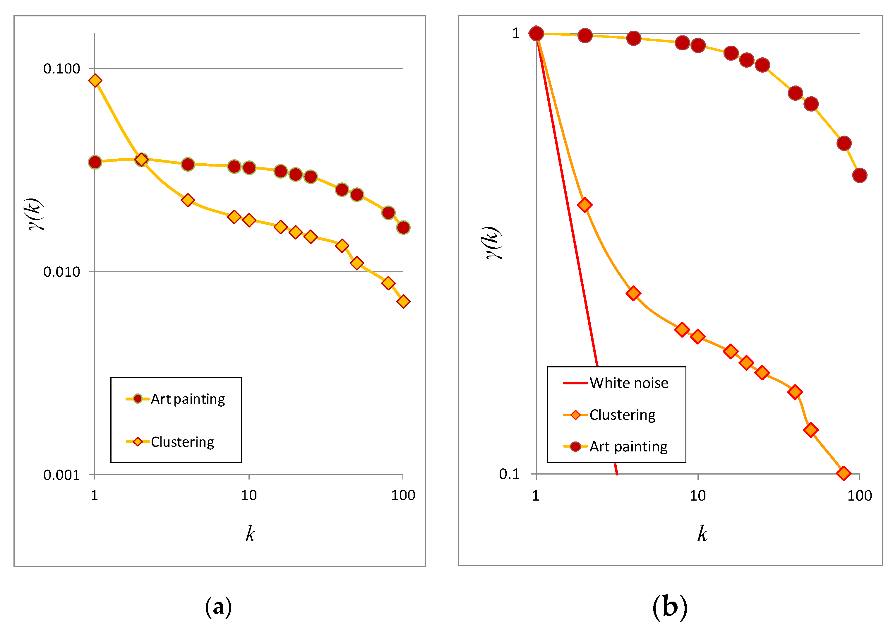
The pixels analyzed are actually represented by numbers based on their grayscale color intensity (white = 1, black = 0). Figure 3 presents three images for benchmark image analysis: (a) white noise; (b) image with clustering; and (c) art painting. Figure 4 presents the steps of analysis and shows grouped pixels at scales k = 2, 4, 8, 16, 20, 25, 40, 50, 80, 100 and 200 used to calculate the climacogram. Figure 5 presents an example of how the data sets of Figure 3 translate into climacograms and standardized climacograms. The latter is defined as the ratio as a function of scale k, and is the basic tool of the 2D-C evaluation process.
The presence of clustering is reflected in the climacogram, which shows a marked difference for the random white noise (Figure 5). Specifically, the variance of the clustered images is notably higher than that of the white noise at all scales, indicating a greater degree of variability of the process. Likewise, comparing the clustered image and the art painting, the latter has the most pronounced clustering behavior and a greater degree of variability.
3. Stochastic Analysis of the Art Paintings
3.1. Stochastic Analysis of the Art Paintings of Leonardo da Vinci (1452–1519) and Pablo Picasso (1881–1973)
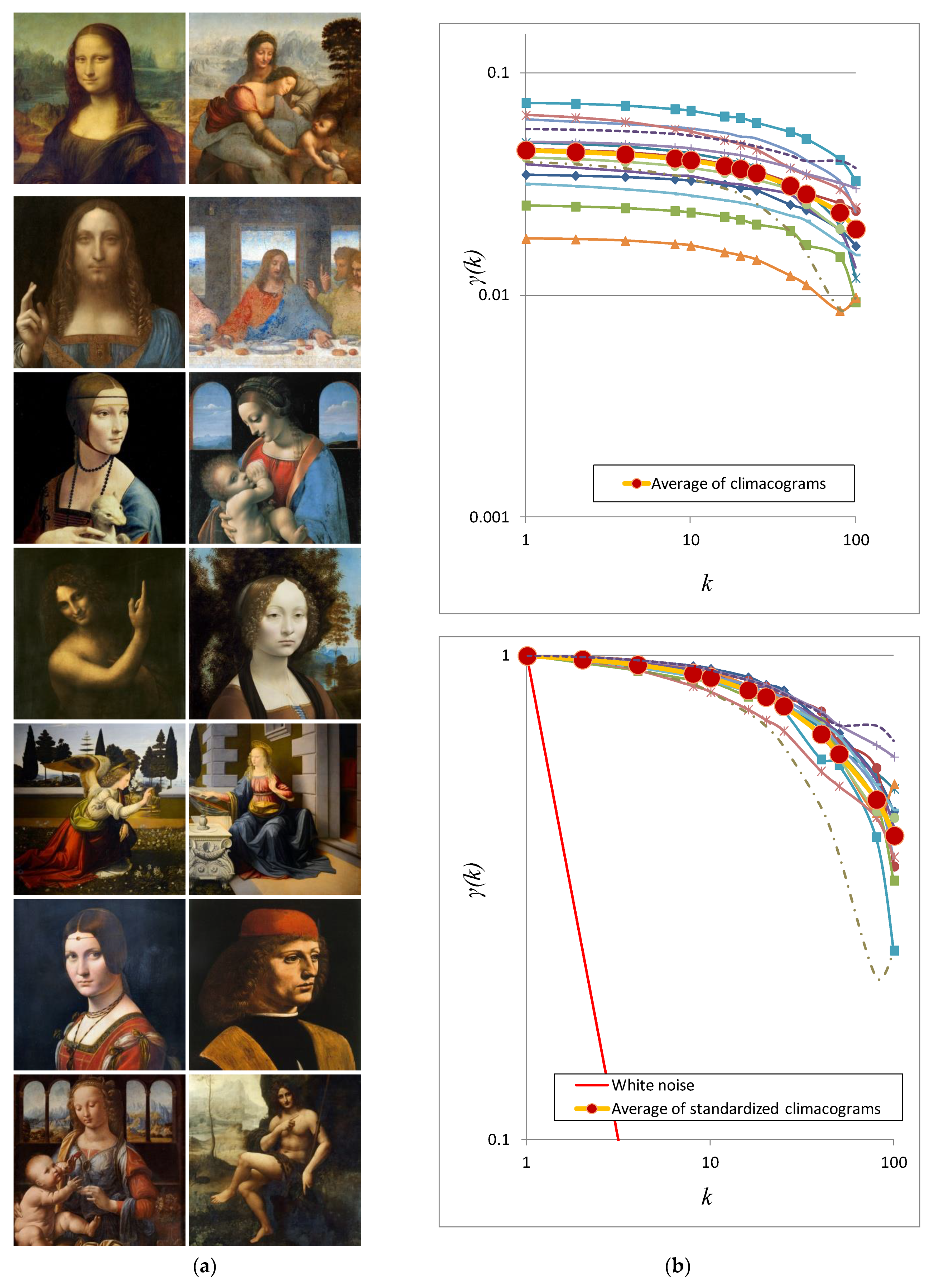
Figure 6.
(a) Paintings of Leonardo da Vinci (1452–1519); (b) Climacograms and standardized climacograms of the paintings; averages thereof are also plotted.
Figure 6.
(a) Paintings of Leonardo da Vinci (1452–1519); (b) Climacograms and standardized climacograms of the paintings; averages thereof are also plotted.

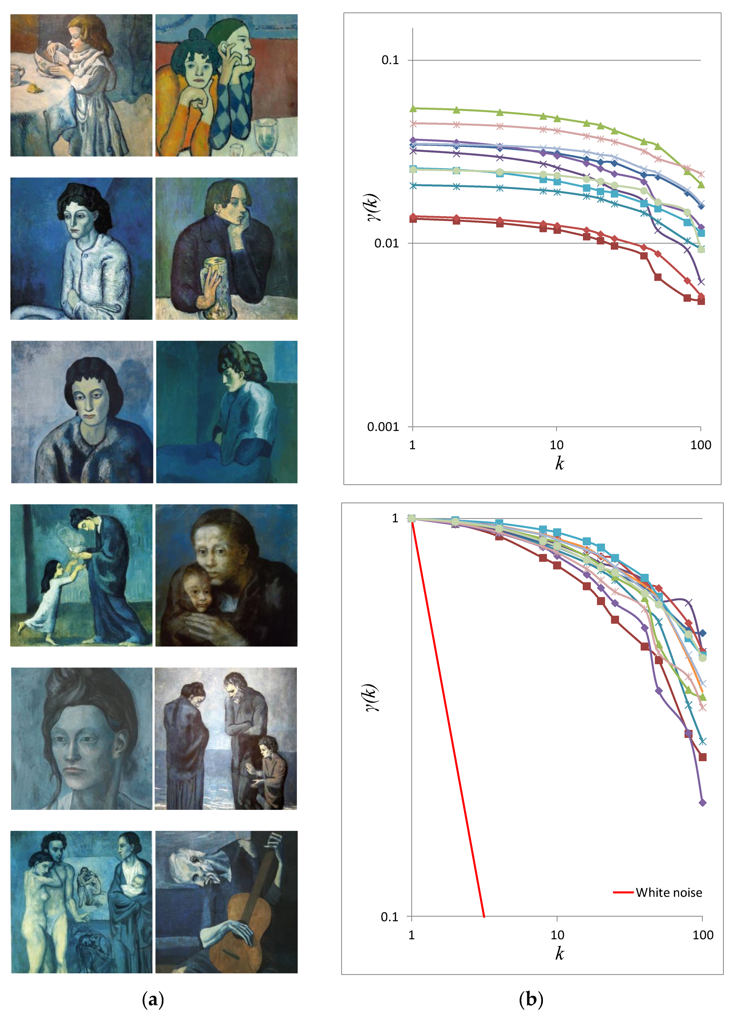
Figure 7.
(a) Paintings of Pablo Picasso in the blue period (1901–1904); (b) Climacograms and standardized climacograms of the paintings.
Figure 7.
(a) Paintings of Pablo Picasso in the blue period (1901–1904); (b) Climacograms and standardized climacograms of the paintings.

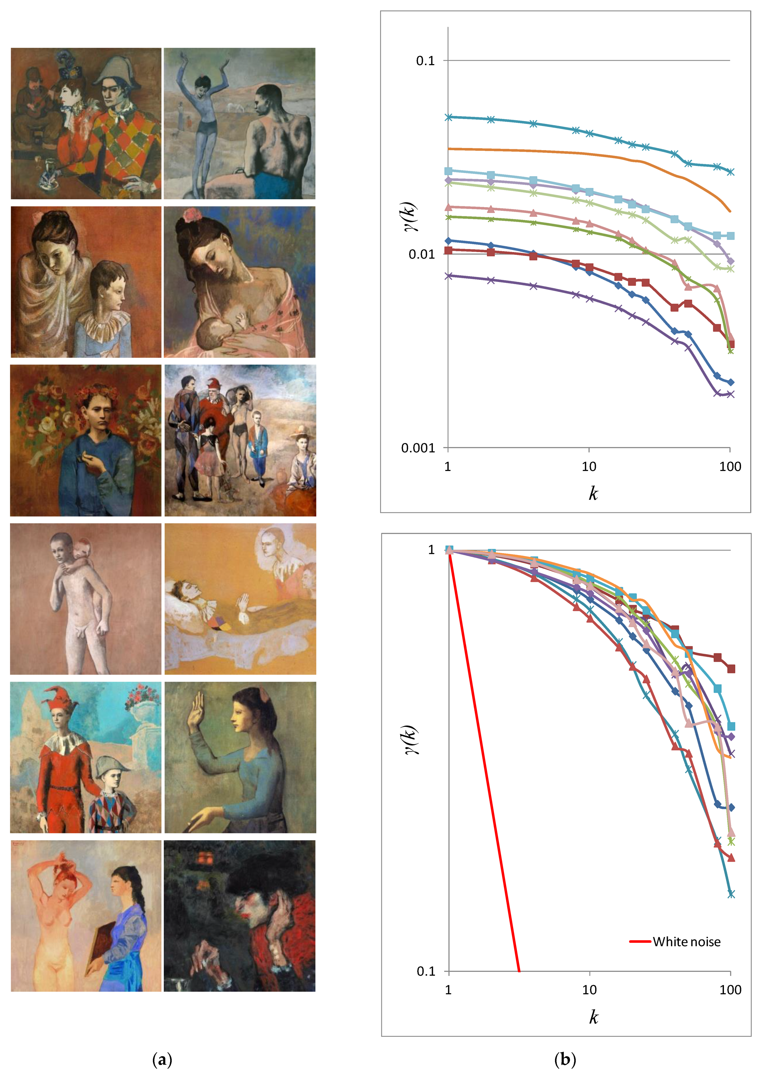
Figure 8.
(a) Paintings of Pablo Picasso in the red period (1904–1906); (b) Climacograms and standardized climacograms of the paintings.
Figure 8.
(a) Paintings of Pablo Picasso in the red period (1904–1906); (b) Climacograms and standardized climacograms of the paintings.

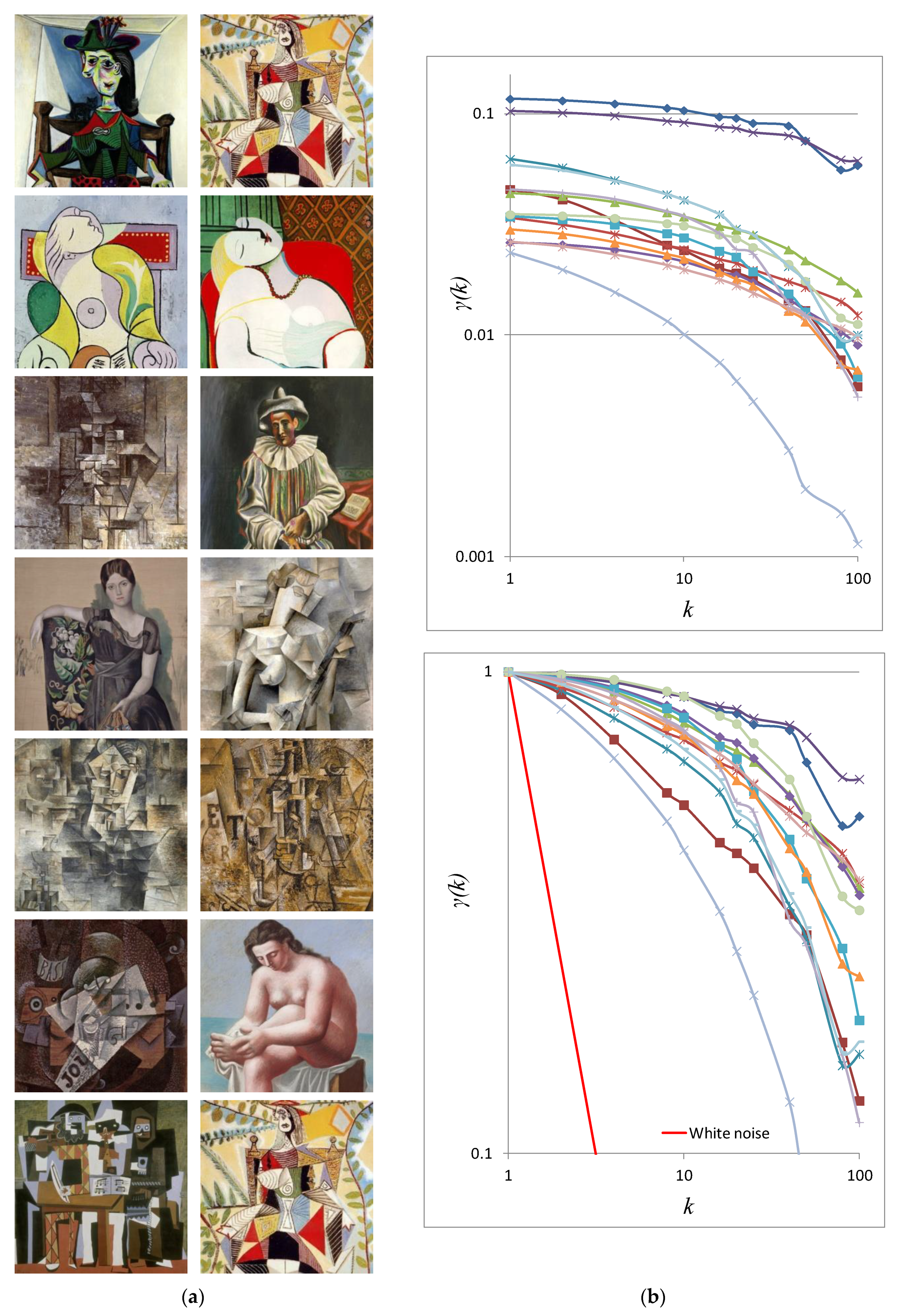
Figure 9.
(a) Paintings of Pablo Picasso after 1910; (b) Climacograms and standardized climacograms of the paintings.
Figure 9.
(a) Paintings of Pablo Picasso after 1910; (b) Climacograms and standardized climacograms of the paintings.

3.2. Stochastic Analysis of of Da Vinci’s Last Supper (1495)
Figure 10.
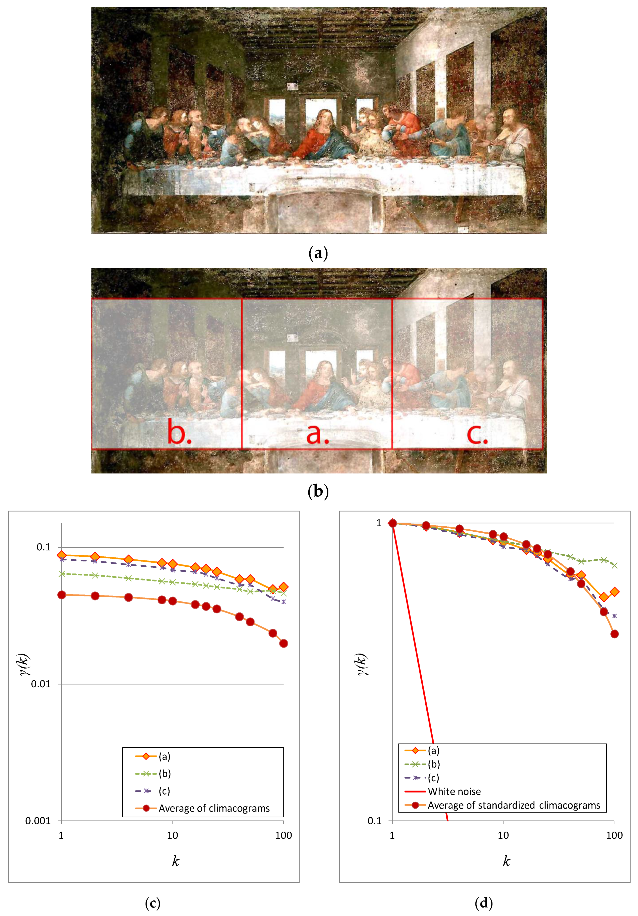
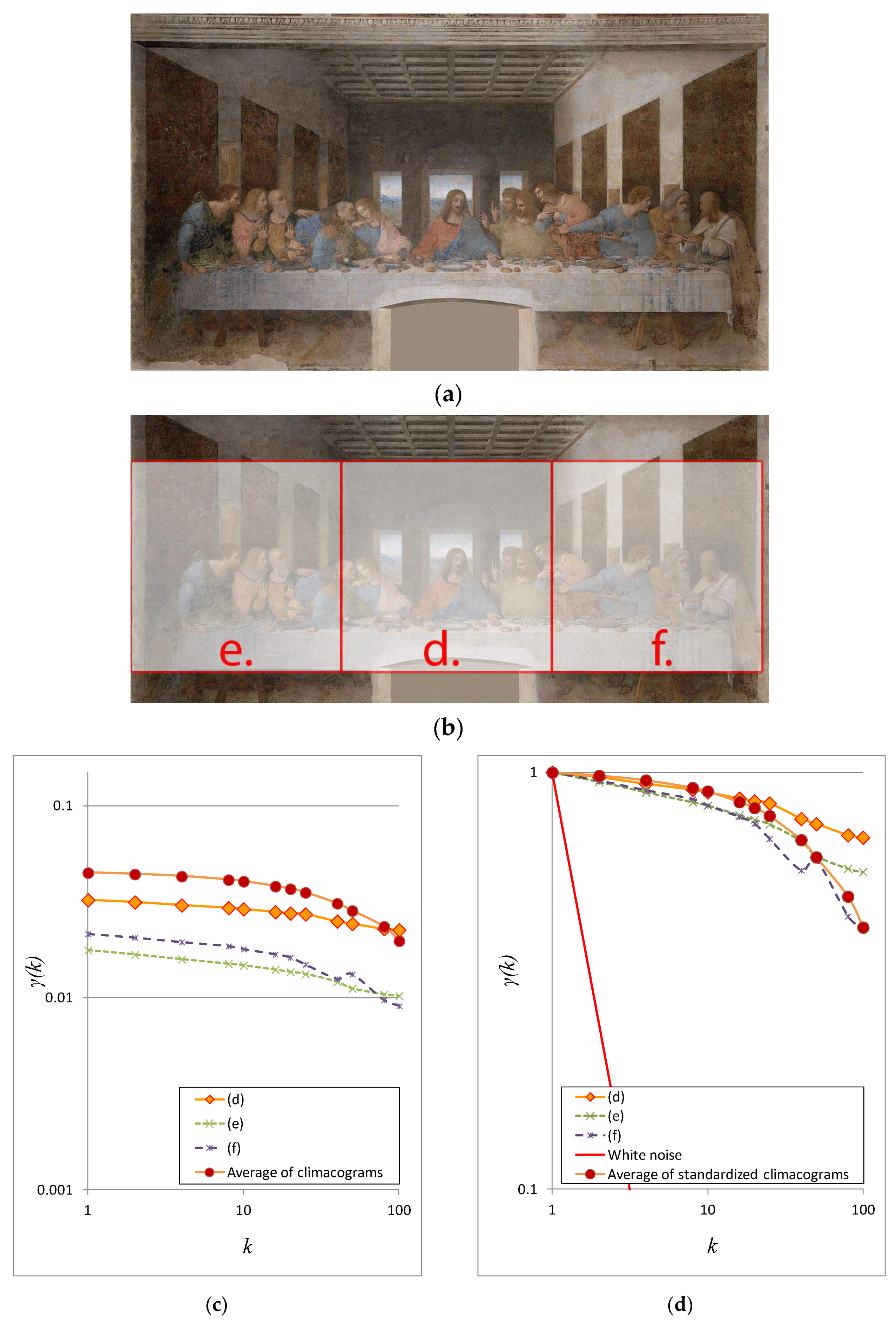
(a) Leonardo da Vinci’s The Last Supper before restoration [83]; (b) Areas of analysis before restoration; (c) Climacograms; (d) Standardized climacograms and averages thereof. Notice that curve of (a) area (center) is between the curves of (b) and (c) areas.
Figure 10.
(a) Leonardo da Vinci’s The Last Supper before restoration [83]; (b) Areas of analysis before restoration; (c) Climacograms; (d) Standardized climacograms and averages thereof. Notice that curve of (a) area (center) is between the curves of (b) and (c) areas.

Figure 11.
(a) Leonardo da Vinci’s The Last Supper after restoration [83]; (b) Areas of analysis after restoration; (c) Climacograms; (d) Standardized climacograms and averages thereof. Notice that curve of (d) area (center) is on top of the curves of (e) and (f) areas.
Figure 11.
(a) Leonardo da Vinci’s The Last Supper after restoration [83]; (b) Areas of analysis after restoration; (c) Climacograms; (d) Standardized climacograms and averages thereof. Notice that curve of (d) area (center) is on top of the curves of (e) and (f) areas.
3.3. Stochastic Analysis of Da Vinci’s Annunciation (1472–1475)
Figure 12.
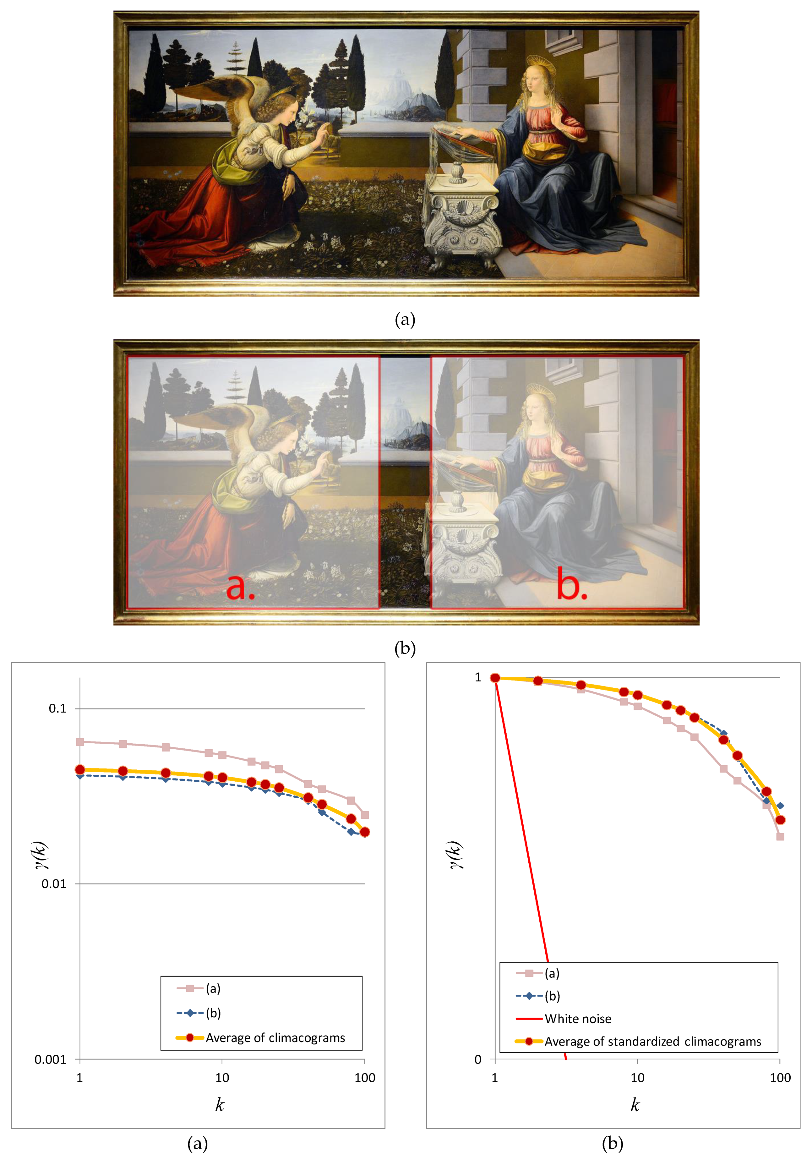
(a) Leonardo da Vinci’s Annunciation; (b) Areas of analysis; (c) Climacograms; (d) standardized climacograms and averages thereof. Notice that curve of (b) area is higher than the curve of (a) area.
Figure 12.
(a) Leonardo da Vinci’s Annunciation; (b) Areas of analysis; (c) Climacograms; (d) standardized climacograms and averages thereof. Notice that curve of (b) area is higher than the curve of (a) area.

3.4. Stochastic Analysis of Da Vinci’s Virgin of the Rocks (1483–1486 and before 1508)
Figure 13.
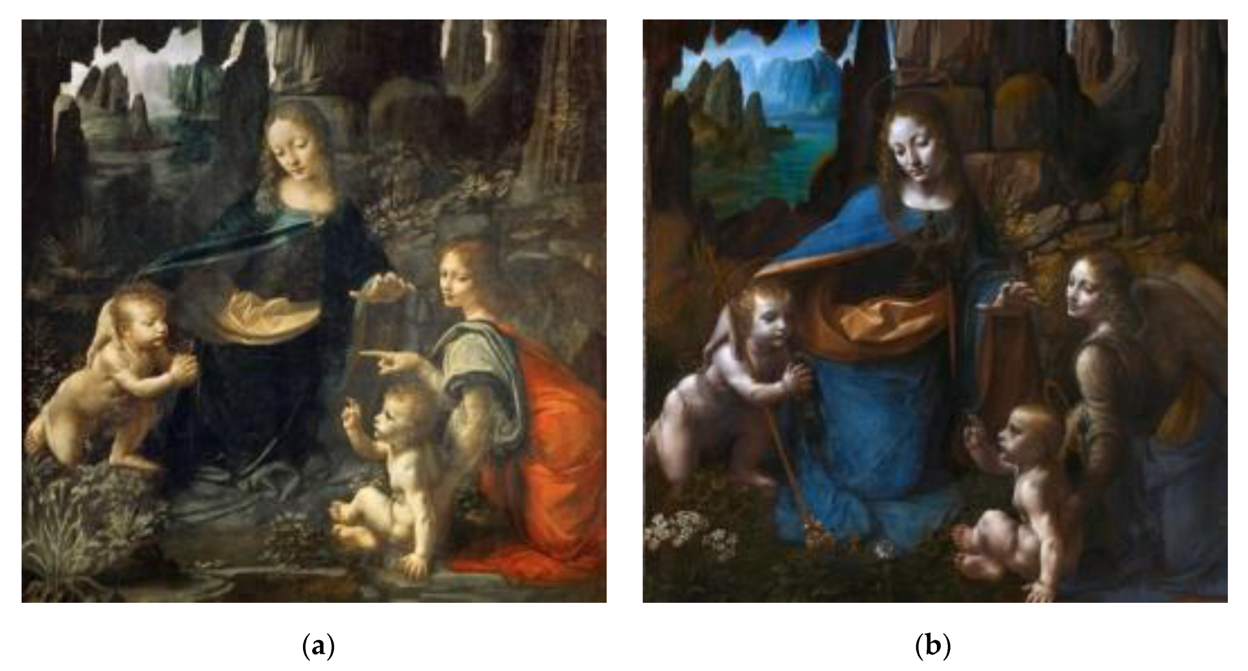
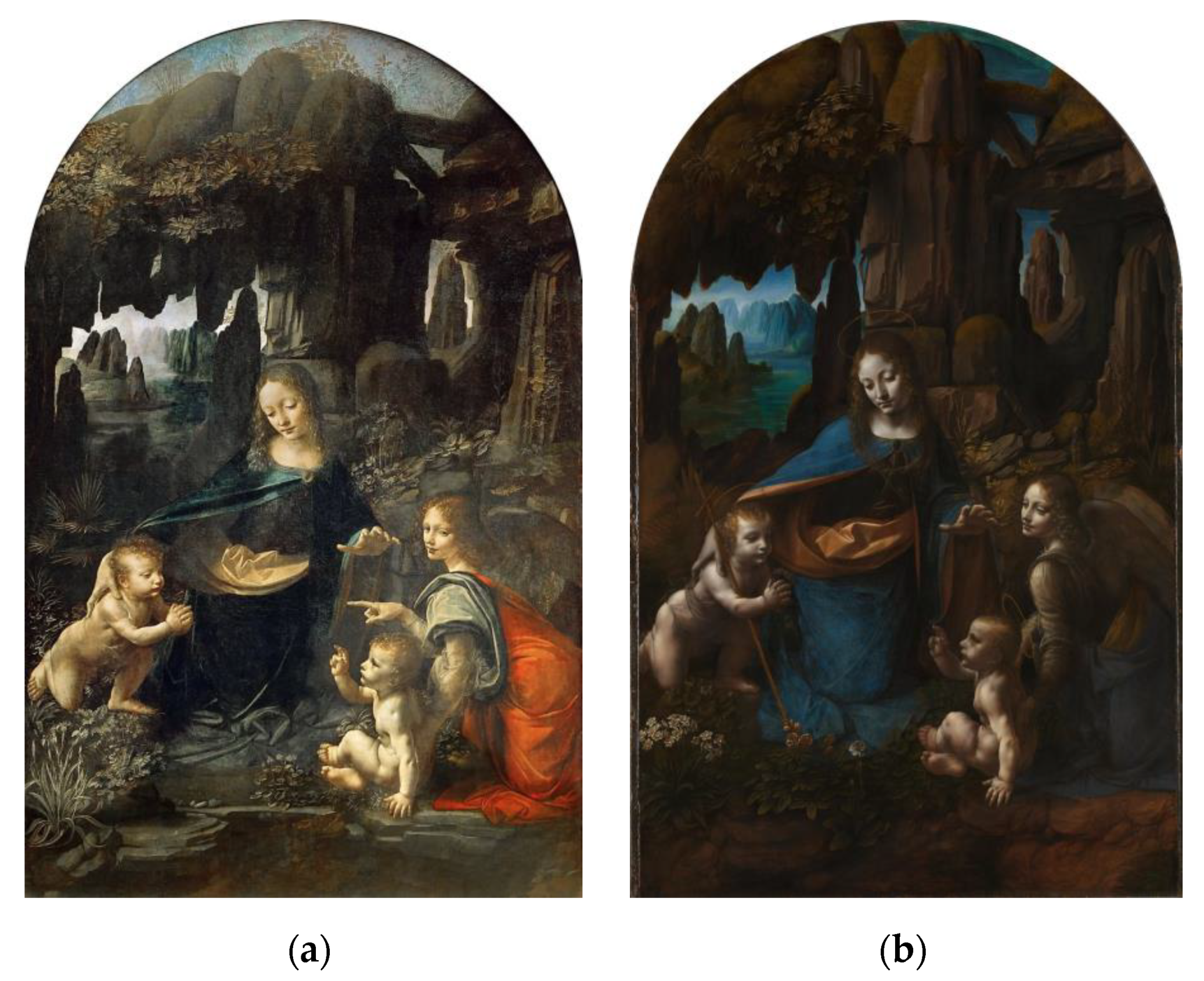
Leonardo da Vinci’s Virgin of the Rocks. Areas of analysis: (a) Louvre version, 1483–1486; (b) National Gallery, London, before 1508.
Figure 13.
Leonardo da Vinci’s Virgin of the Rocks. Areas of analysis: (a) Louvre version, 1483–1486; (b) National Gallery, London, before 1508.

Figure 14.
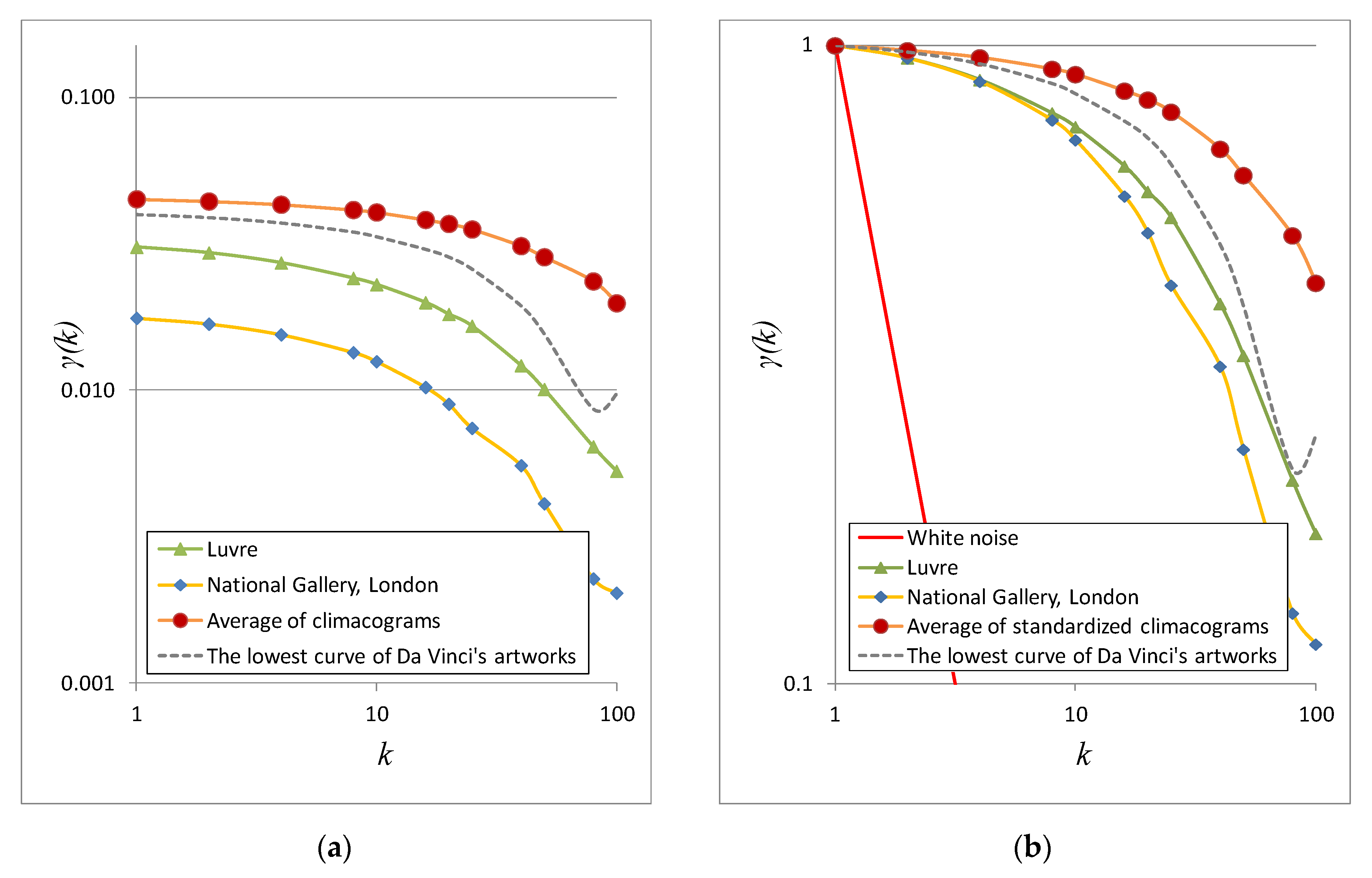
(a) Climacograms; (b) standardized climacograms of Leonardo da Vinci’s Virgin of the Rocks and averages thereof. Notice that curve of the Louvre version is closer to the average of standardized climacograms of the National Gallery of London version.
Figure 14.
(a) Climacograms; (b) standardized climacograms of Leonardo da Vinci’s Virgin of the Rocks and averages thereof. Notice that curve of the Louvre version is closer to the average of standardized climacograms of the National Gallery of London version.

Figure 15.
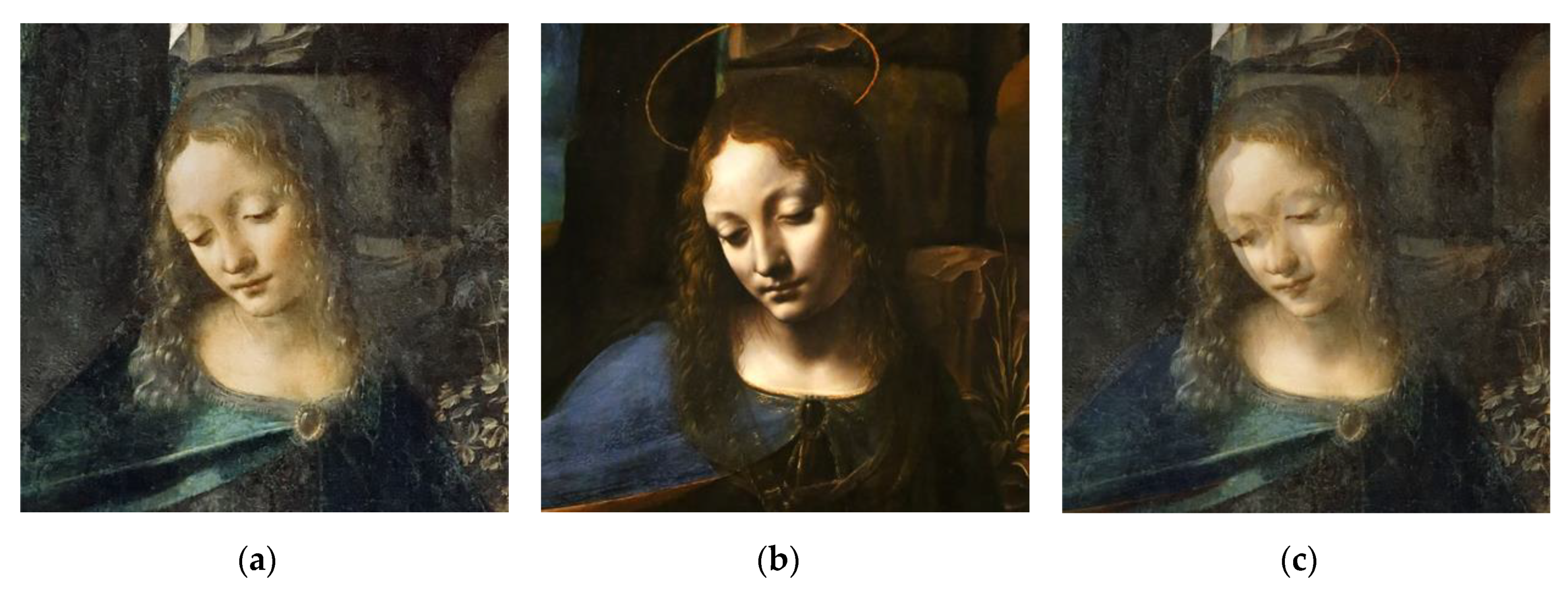
Leonardo da Vinci’s Virgin of the Rocks, Madonna. Areas of analysis: (a) Louvre version, 1483–1486; (b) National Gallery of London, before 1508; (c) Preparation of analyzing (one image over the other).
Figure 15.
Leonardo da Vinci’s Virgin of the Rocks, Madonna. Areas of analysis: (a) Louvre version, 1483–1486; (b) National Gallery of London, before 1508; (c) Preparation of analyzing (one image over the other).

Figure 16.
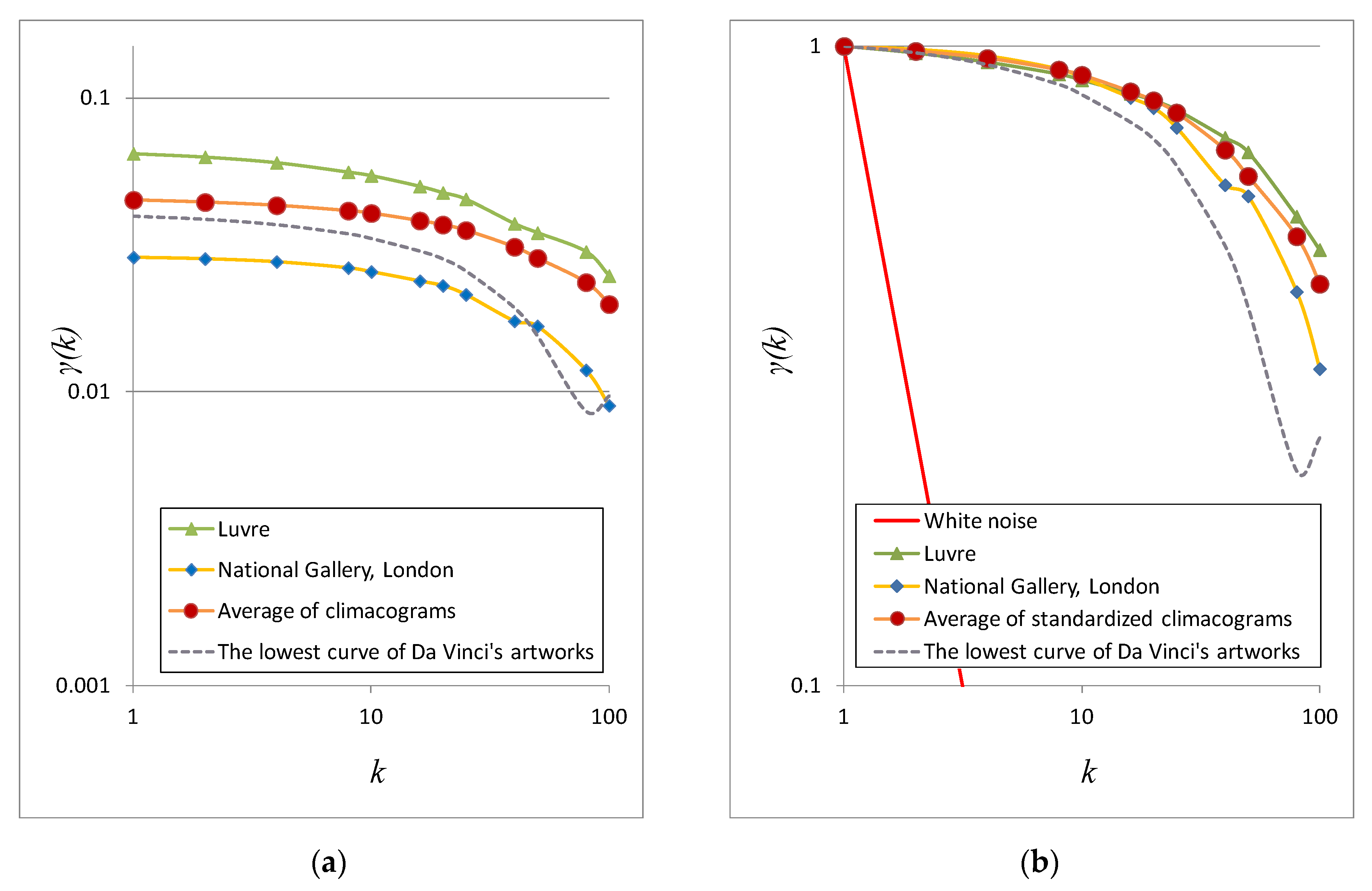
(a) Climacograms; (b) standardized climacograms of Leonardo da Vinci’s Virgin of the Rocks (Madonna), and averages thereof. Notice that curve of Louvre version is closer to the average of standardized climacograms of Da Vinci’s artworks than the curve of National Gallery of London.
Figure 16.
(a) Climacograms; (b) standardized climacograms of Leonardo da Vinci’s Virgin of the Rocks (Madonna), and averages thereof. Notice that curve of Louvre version is closer to the average of standardized climacograms of Da Vinci’s artworks than the curve of National Gallery of London.

Figure 17.
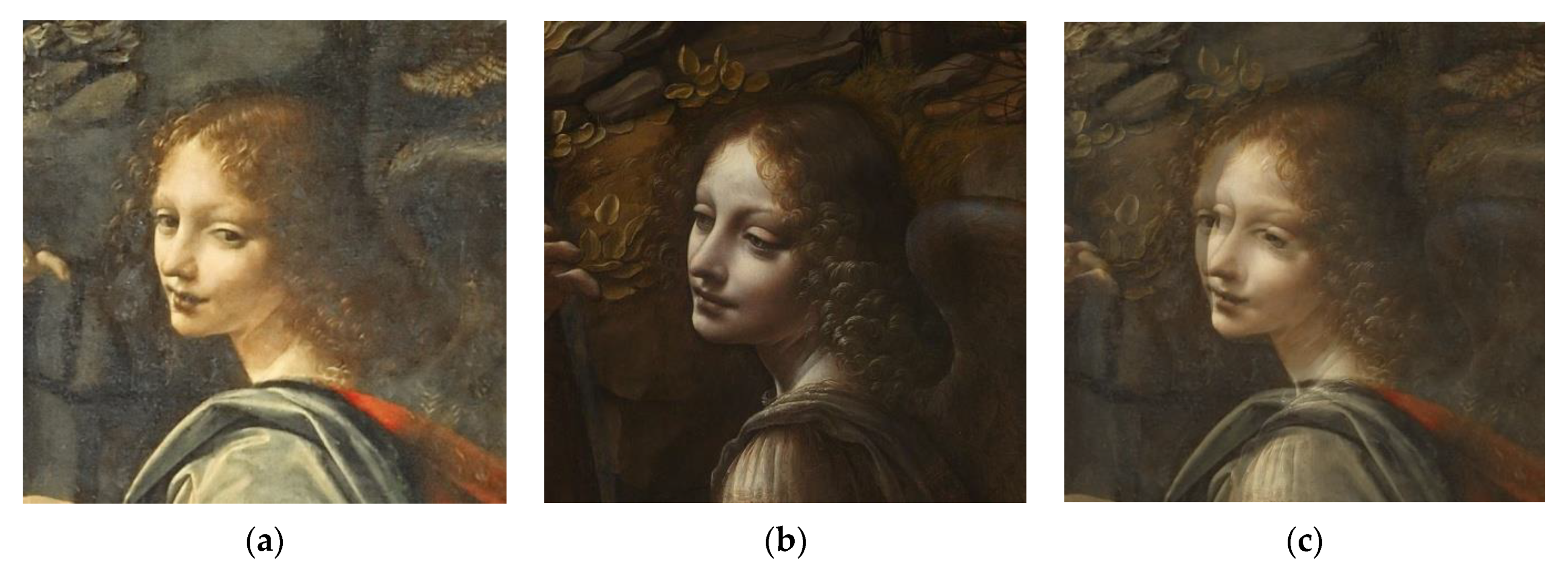
Leonardo da Vinci’s Virgin of the Rocks, Angel. Areas of analysis: (a) Louvre version, 1483–1486; (b) National Gallery of London, before 1508; (c) Preparation of analyzing (one image over the other).
Figure 17.
Leonardo da Vinci’s Virgin of the Rocks, Angel. Areas of analysis: (a) Louvre version, 1483–1486; (b) National Gallery of London, before 1508; (c) Preparation of analyzing (one image over the other).

Figure 18.
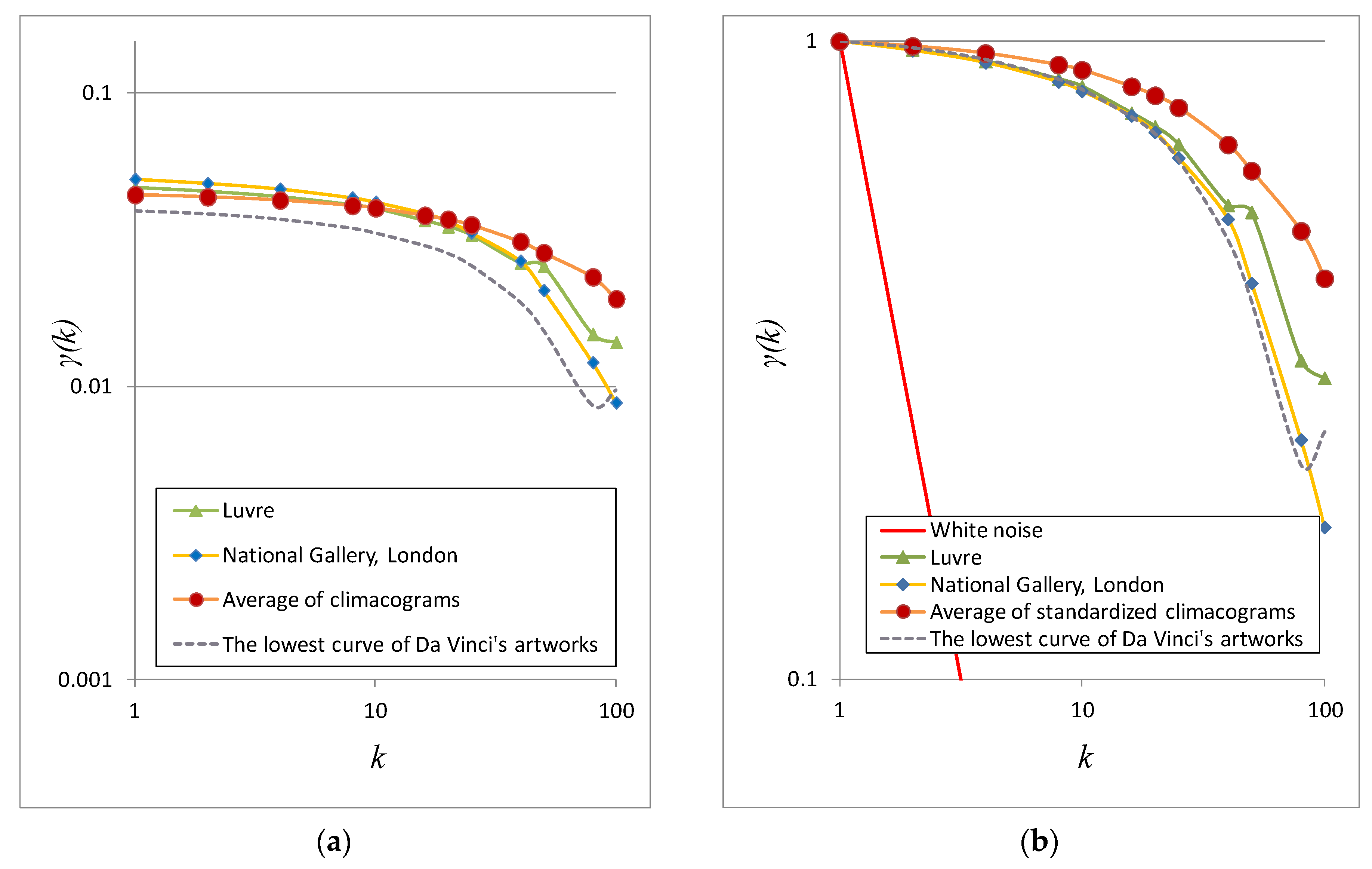
(a) Climacograms; (b) standardized climacograms of Leonardo da Vinci’s Virgin of the Rocks (Angel), and averages thereof. Notice that curve of Louvre version is closer to the average of standardized climacograms of Da Vinci’s artworks than the curve of National Gallery of London.
Figure 18.
(a) Climacograms; (b) standardized climacograms of Leonardo da Vinci’s Virgin of the Rocks (Angel), and averages thereof. Notice that curve of Louvre version is closer to the average of standardized climacograms of Da Vinci’s artworks than the curve of National Gallery of London.

4. Discussion of Stochastic Evaluation
4.1. Stochastic Evaluation of Da Vinci’s and Picasso’s Art Paintings
Leonardo da Vinci (1452–1519) and Pablo Picasso (1881–1973) were two great artists who lived in different periods and had different artworks styles. Both have greatly influenced arts [84,85,86], and therefore, here, we have selected these two to quantify the variability of their works, searching for stochastic similarities among their paintings.
For each painting, we calculated the coefficient of variation of the original image at scale 1, which, by definition, is the standard deviation of brightness divided by the average. We then calculated the average of all the paintings of each artist. A high value of the coefficient of variation shows that an artist uses a broad range of brightness in his paintings for the same average brightness. The average coefficient of variation of Da Vinci’s artworks is equal to 0.7 and that of Picasso’s artworks is equal to 0.45.
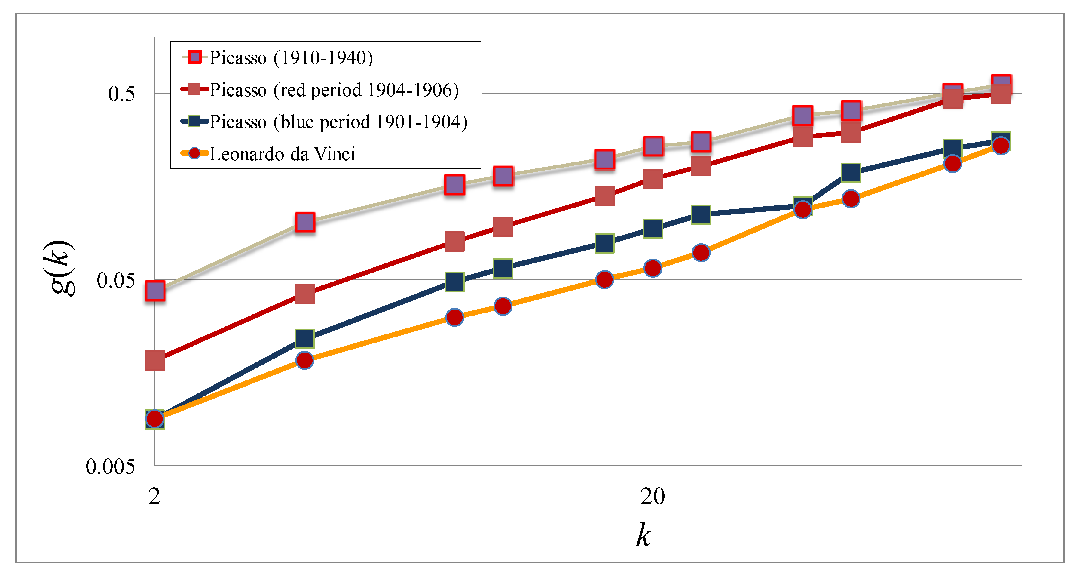
In order to see the range of fluctuations of climacograms, for each scale k we calculated the coefficient of variation of all standardized climacograms, g(k). As we have seen in Figure 6, the art paintings of Leonardo da Vinci exhibit stochastic similarity, and he has his own steady stochastic canon of expression, which is represented by a stochastic Golden Climacogram. In contrast, Picasso’s artworks (in stochastic view) display a wide range of fluctuations (Figure 7, Figure 8 and Figure 9). Figure 19 shows the graphs of g(k) vs. k for all examined cases. This range of fluctuations is larger as the artist growing older.
Analyzing Figure 19, we could say that Da Vinci’s art paintings are more stable and Picasso’s have more fluctuation. Picasso’s artworks were more fuzzy as the artist was growing older, with bigger and bigger variance.
4.2. Stochastic Evaluation of the Restoration of Da Vinci’s Last Supper
In 1495, Leonardo da Vinci began what would become one of history’s most influential works of art—The Last Supper (Italian: Ultima Cena) [87].
The Last Supper is regarded as one of Leonardo da Vinci’s masterpieces, [88] but twenty years after its completion, the painting began to chip and fade. Unlike traditional frescoes, which Renaissance masters painted on wet plaster walls, da Vinci experimented with tempura paint on a dry, sealed plaster. The experiment proved unsuccessful, however, because the paint did not adhere properly and began to flake away only a few decades after the work was finished. Da Vinci’s masterpiece has been subject to numerous restoration attempts. Some of these took place in 1726, 1770, 1853, 1903, 1924, 1928 and 1978. [89]. Critics maintain that only a fraction of the painting that exists today is the work of Leonardo da Vinci. [90,91,92].
Stochastic analysis of Da Vinci’s Last Supper shows that the curve of the center area (curve (a), Figure 10d) before restoration is between the others, but after restoration is above the others (curve (d), Figure 11d). The coefficient of variation before restoration was 2.3 and after restoration became 2.6, while the average of Da Vinci’s artwork is 3.4. We could thus say that after restoration Last Supper’s Coefficient of Variation came closer to Da Vinci’s artworks. All the curves are very close to Da Vinci’s stochastic Golden Climacogram. Thus, it seems that Last Supper after restoration is, from the stochastic view, more intense in the center, which makes sense as obviously the artist would like to give emphasis to the center of the painting. So, the answer to the question “was the restoration of Last Supper successful?” seems to be positive.
4.3. Stochastic Evaluation of Da Vinci’s Annunciation
Leonardo Da Vinci’s Annunciation (Figure 12a) is dated circa 1472–1475. It is housed in the Uffizi gallery of Florence, Italy [93,94].
Stochastic analysis in specific areas of Da Vinci’s Annunciation (Figure 12b) (1472–1475) shows that the area of the angel (curve (a), Figure 12c,d) is clearly different than the area of Madonna (curve (b), Figure 12c,d). We could say that the artist might want to show a move from divine (angel) to humanity (Madonna).
4.4. Stochastic Evaluation of Da Vinci’s Virgin of the Rocks
The Virgin of the Rocks (Italian: Vergine delle rocce; sometimes the Madonna of the Rocks) is the name of two paintings by Leonardo da Vinci, of the same subject, and of a composition which is identical except for several significant details. The version generally regarded as the prime version, the earlier of the two, is in the Louvre in Paris and is not restored (Figure 20a). The other is in the National Gallery in London, and it was restored between 2008 and 2010 (Figure 20b) [95].
Both paintings are ascribed to Leonardo da Vinci. Originally, they were thought to have been partially painted by Leonardo’s assistants. A close look at the painting during the recent restoration has led the conservators from the National Gallery to conclude that the greater part of the work is by the hand of Leonardo, but debate continues [96,97]. Parts of the painting, the flowers in particular, indicate the collaboration, and have led to speculation that the work is entirely by other hands, possibly Leonardo’s assistant Giovanni Ambrogio de Predis, and perhaps Evangelista [95].
A general view, with stochastic analysis, of Da Vinci’s Virgin of the Rocks (Figure 13) shows that, even though both of the art paintings are far enough from Da Vinci’s stochastic forms, the Louvre version is closer to Da Vinci’s stochastic Golden Climacogram (Figure 14). A closer view in the frames of Madonna (Figure 15) and Angel (Figure 17) shows that, in stochastic terms, both of them are very close to Da Vinci’s stochastic Golden Climacogram, and the Louvre version is closer to Da Vinci’s stochastic Golden Climacogram (Figure 16 and Figure 18). Thus, we could make the conjecture that the wider drawing of the painting has been done by someone else, and these details by Da Vinci.
5. Conclusions
Modern mathematical tools and artificial intelligence provide many computational methods for evaluation and classification. Some of them use scale-variant methods similar to 2D-C, but with very complex processes and algorithms which could not be understood by a non-expert.
2D-C presents a clear and simple quantification tool based on the climacogram, a simple means of mathematic evaluation of art paintings, the results of which could be understood by a non-expert, and could provide insights into the aesthetical study of an art painting, as seen in the examples of this study.
With 2D-C, stochastic patterns can be observed in terms of the dependence structure among the different artists as well, with Da Vinci’s (average H ≈ 0.84) and Picasso’s (average H ≈ 0.85) artworks having a strong persistence structure.
Interestingly, similar Hurst parameters, between the range of 0.8 and 0.9, are estimated by Hurst in his pioneering work on the stage of the river Nile [98,99,100] and, additionally, in global-scale analyses of the long annual records of key hydrometeorological processes (such as temperature and wind speed) as well as of small-scale processes recorded in the laboratory (such as grid-turbulence and turbulent jets) [63]. Thus, a philosophical issue arises from the above analysis: does the inherent uncertainty in arts suggest some similarity with physical phenomena?
From the analysis above we found that, in contrast to Picasso, Da Vinci had a stochastically steady way of expression (Golden Climacogram). An interesting study for further analysis would be to find out if other artists have stochastic similarities among their artwork, and to research if there are correlations among them.
Author Contributions
Conceptualization, G.-F.S.; methodology, G.-F.S., P.D. and D.K.; software, P.D.; validation, G.-F.S.; formal analysis, G.-F.S., P.D.; investigation, G.-F.S.; data processing, G.-F.S.; writing—original draft preparation, G.-F.S.; writing—review and editing, D.K.; visualization, G.-F.S.; supervision, D.K.; project administration, D.K. All authors have read and agreed to the published version of the manuscript.
Funding
This research received no external funding.
Acknowledgments
We are grateful to the editor and two anonymous reviewers for their positive critique and their constructive comments. As this paper was prepared, submitted and accepted during lock-down from COVID-19 (March–April 2020), G.F.S would like to thank his daughters Maria-Artemis and Eleni-Angelina for their patience.
Conflicts of Interest
The authors declare no conflict of interest.
References
- Bullot, N.J.; Seeley, W.P.; Davies, S. Art and Science: A Philosophical Sketch of Their Historical Complexity and Codependence. J. Aesthet. Art Crit. 2017, 75, 453–463. [Google Scholar] [CrossRef]
- Robins, G. Proportion and Style in Ancient Egyptian Art; University of Texas Press: Austin, TX, USA, 1994. [Google Scholar]
- The Sculptor’s Funeral. Available online: www.thesculptorsfuneral.com/episode-05-canons-of-proportion/ (accessed on 21 April 2020).
- Canons of Proportion and the Laws of Nature: Observations on a Permanent and Unresolved Conflict. Arch. Hist. 2014, 2, 19. [CrossRef]
- Riedel, T. Encyclopedia of Aesthetics. Art Doc. J. Art Libr. Soc. N. Am. 1999, 18, 48. [Google Scholar] [CrossRef]
- Thapa, G.B.; Thapa, R. The Relation of Golden Ratio, Mathematics and Aesthetics. J. Inst. Eng. 2018, 14, 188–199. [Google Scholar] [CrossRef]
- Schreiber, P. A Supplement to J. Shallit’s Paper “Origins of the Analysis of the Euclidean Algorithm”. Hist. Math. 1995, 22, 422–424. [Google Scholar] [CrossRef] [Green Version]
- Kennick, W.E.; Beardsley, M.C. Aesthetics from Classical Greece to the Present: A Short History. Philos. Rev. 1969, 78, 270. [Google Scholar] [CrossRef]
- Bulent, A. Math and the Mona Lisa: The Art and Science of Leonardo da Vinci; Simthsonian Institution: London, UK, 2014. [Google Scholar]
- Akhtaruzzaman Shafie, A.A. Geometrical Substantiation of Phi, the Golden Ratio and the Baroque of Nature, Architecture, Design and Engineering. Int. J. Arts 2012, 1, 1–22. [Google Scholar] [CrossRef] [Green Version]
- Omotehinwa, T.O.; Ramon, S.O. Fibonacci Numbers and Golden Ratio in Mathematics and Science. Int. J. Comput. Inf. Technol. 2013, 630–638. [Google Scholar]
- Liu, C.-H.; Ting, C.-K. Polyphonic accompaniment using genetic algorithm with music theory. In Proceedings of the IEEE Congress on Evolutionary Computation, Brisbane, QLD, Australia, 10–15 June 2012; pp. 1–7. [Google Scholar] [CrossRef] [Green Version]
- Liu, C.-H.; Ting, C.-K. Evolutionary composition using music theory and charts. In Proceedings of the IEEE Symposium on Computational Intelligence for Creativity and Affective Computing (CICAC), Singapore, 16–19 April 2013; pp. 63–70. [Google Scholar] [CrossRef]
- McIntyre, R.A. Bach in a box: The evolution of four part Baroque harmony using the genetic algorithm. In Proceedings of the First IEEE Conference on Evolutionary Computation. IEEE World Congress on Computational Intelligence, Orlando, FL, USA, 27–29 June 2002; Volume 2, pp. 852–857. [Google Scholar]
- Pazos, A.; Del Riego, A.S.; Dorado, J.; Caldalda, J.R. Genetic music compositor. In Proceedings of the 1999 Congress on Evolutionary Computation-CEC99 (Cat. No. 99TH8406), Washington, DC, USA, 6–9 July 2003; Volume 2, pp. 885–890. [Google Scholar] [CrossRef]
- Fogel, D. Imagining machines with imagination. Proc. IEEE 2000, 88, 284–288. [Google Scholar] [CrossRef]
- Feng, S.-Y.; Ting, C.-K. Painting Using Genetic Algorithm with Aesthetic Evaluation of Visual Quality. In Computer Vision; Springer Science and Business Media LLC: Berlin, Germany, 2014; Volume 8916, pp. 124–135. [Google Scholar]
- Berlyne, D.E. (Ed.) Studies in the New Experimental Aesthetics: Steps Toward an Objective Psychology of Aesthetic Appreciation; Hemisphere: New York, NY, USA, 1974. [Google Scholar]
- Fayn, K.; Silvia, P.J.; Erbas, Y.; Tiliopoulos, N.; Kuppens, P. Nuanced aesthetic emotions: Emotion differentiation is related to knowledge of the arts and curiosity. Cogn. Emot. 2017, 32, 593–599. [Google Scholar] [CrossRef] [PubMed]
- Mulkay, M.; Chaplin, E. Aesthetics and the Artistic Career: A Study of Anomie in Fine-Art Painting. Sociol. Q. 1982, 23, 117–138. [Google Scholar] [CrossRef]
- Gordon, D.A. Methodology in the Study of Art Evaluation. J. Aesthet. Art Crit. 1952, 10, 338. [Google Scholar] [CrossRef]
- Bourgeon, D. Evaluating Consumer Behaviour in the Field of Arts and Culture Marketing. Int. J. Arts Manag. 2000, 3, 4–18. [Google Scholar]
- Lombardi, T.E. The Classification of Style in Fine-Art Painting, School of Computer Science and Information Systems; Pace University: New York, NY, USA, 2005. [Google Scholar]
- Thomasson, A.L. The Ontology of Art and Knowledge in Aesthetics. J. Aesthet. Art Crit. 2005, 63, 221–229. [Google Scholar] [CrossRef]
- Swami, V. Context matters: Investigating the impact of contextual information on aesthetic appreciation of paintings by Max Ernst and Pablo Picasso. Psychol. Aesthet. Creat. Arts 2013, 7, 285–295. [Google Scholar] [CrossRef]
- Winston, A.S.; Gerald, C.C. The Evaluation of High Art and Popular Art by Naive and Experienced Viewers. Vis. Arts Res. 1992, 18, 1–14. [Google Scholar]
- De Caro, L.; Matricciani, E.; Fanti, G. Imaging Analysis and Digital Restoration of the Holy Face of Manoppello—Part II. Heritage 2018, 1, 349–364. [Google Scholar] [CrossRef] [Green Version]
- Augello, A.; Infantino, I.; Maniscalco, U.; Pilato, G.; Rizzo, R.; Vella, F. Robotic intelligence and computational creativity. Encycl. Semant. Comput. Robot. Intell. 2018, 2, 1850011. [Google Scholar] [CrossRef]
- Carbonneau, M.-A.; Cheplygina, V.; Granger, E.; Gagnon, G. Multiple instance learning: A survey of problem characteristics and applications. Pattern Recognit. 2018, 77, 329–353. [Google Scholar] [CrossRef]
- Carballal, A.; Santos, A.; Romero, J.; Machado, F.J.P.M.; Correia, J.; Castro, L. Distinguishing paintings from photographs by complexity estimates. Neural Comput. Appl. 2016, 30, 1957–1969. [Google Scholar] [CrossRef]
- Castellano, G.; Vessio, G. Towards a Tool for Visual Link Retrieval and Knowledge Discovery in Painting Datasets. In Communications in Computer and Information Science; Springer Science and Business Media LLC: Berlin, Germany, 2020; Volume 1177, pp. 105–110. [Google Scholar]
- Collomosse, J.; Bui, T.; Wilber, M.; Fang, C.; Jin, H. Sketching with Style: Visual Search with Sketches and Aesthetic Context. In Proceedings of the 2017 IEEE International Conference on Computer Vision (ICCV), Venice, Italy, 22–29 October 2017; pp. 2679–2687. [Google Scholar]
- Leonov, S.C.; Vasilyev, A.; Makovetskii, A.; Diaz-Escobar, J. An algorithm of face recognition based on generative adversarial networks. Appl. Digit. Image Process. Xli 2018, 10752, 107522L. [Google Scholar] [CrossRef]
- Jboor, N.H.; Belhi, A.; Al-Ali, A.K.; Bouras, A.; Jaoua, A. Towards an Inpainting Framework for Visual Cultural Heritage. In Proceedings of the 2019 IEEE Jordan International Joint Conference on Electrical Engineering and Information Technology (JEEIT), Amman, Jordan, 9–11 April 2019; pp. 602–607. [Google Scholar]
- Correia, J.; Machado, P.; Romero, J.; Martins, P.; Cardoso, A.F. Breaking the Mould An Evolutionary Quest for Innovation Through Style Change. In Concept Invention; Springer Science and Business Media LLC: Berlin, Germany, 2019; pp. 353–398. [Google Scholar]
- Neumann, A.; Alexander, B.; Neumann, F. Evolutionary Image Transition and Painting Using Random Walks. Evol. Comput. 2020, 28, 1–34. [Google Scholar] [CrossRef] [PubMed] [Green Version]
- Shen, J. Stochastic modeling western paintings for effective classification. Pattern Recognit. 2009, 42, 293–301. [Google Scholar] [CrossRef]
- Florea, C.; Gieseke, F. Artistic movement recognition by consensus of boosted SVM based experts. J. Vis. Commun. Image Represent. 2018, 56, 220–233. [Google Scholar] [CrossRef]
- Tan, W.R.; Chan, C.S.; Aguirre, H.; Tanaka, K. Ceci n’est pas une pipe: A deep convolutional network for fine-art paintings classification. In Proceedings of the 2016 IEEE International Conference on Image Processing (ICIP), Phoenix, AZ, USA, 25–28 September 2016; pp. 3703–3707. [Google Scholar]
- Van Noord, N.; Postma, E. Learning scale-variant and scale-invariant features for deep image classification. Pattern Recognit. 2017, 61, 583–592. [Google Scholar] [CrossRef] [Green Version]
- Tan, W.R.; Chan, C.S.; Aguirre, H.; Tanaka, K. ArtGAN: Artwork synthesis with conditional categorical GANs. In Proceedings of the 2017 IEEE International Conference on Image Processing (ICIP), Beijing, China, 17–20 September 2017; pp. 3760–3764. [Google Scholar]
- Fuchs, R.; Hauser, H. Visualization of Multi-Variate Scientific Data. Comput. Graph. Forum 2009, 28, 1670–1690. [Google Scholar] [CrossRef]
- Trends in Information Visualization, An Overview of Current Trends, Development and Research in Information Visualization; Technical Report LMU-MI-2010-1; University of Munich, Department of Computer Science Media Informatics Group: Munich, Germany, 2010; Available online: http://141.84.8.93/pubdb/publications/pub/baur2010infovisHS/baur2010infovisHS.pdf#page=16 (accessed on 21 April 2020).
- Lecoutre, A.; Negrevergne, B.; Yger, F. Recognizing Art Style Automatically in Painting with Deep Learning. JMLR Workshop Conf. Proc. 2017, 80, 1–17. Available online: https://www.lamsade.dauphine.fr/~bnegrevergne/webpage/documents/2017_rasta.pdf (accessed on 21 April 2020).
- Cetinic, E.; Lipic, T.; Grgic, S. Fine-tuning Convolutional Neural Networks for fine art classification. Expert Syst. Appl. 2018, 114, 107–118. [Google Scholar] [CrossRef]
- Cetinic, E.; Lipic, T.; Grgic, S. Learning the Principles of Art History with convolutional neural networks. Pattern Recognit. Lett. 2020, 129, 56–62. [Google Scholar] [CrossRef]
- Babak, S.; Elgammal, A. Large-Scale Classification of Fine-Art Paintings: Learning the Right Metric on the Right Feature. Int. J. Digit. Art Hist. 2016, 2, 70–93. [Google Scholar]
- Sandoval, C.; Pirogova, E.; Lech, M. Two-Stage Deep Learning Approach to the Classification of Fine-Art Paintings. IEEE Access 2019, 7, 41770–41781. [Google Scholar] [CrossRef]
- Wang, Z.; Lian, J.; Song, C.; Zhang, Z.; Zheng, W.; Yue, S.; Ji, S. SAS: Painting Detection and Recognition via Smart Art System with Mobile Devices. IEEE Access 2019, 7, 135563–135572. [Google Scholar] [CrossRef]
- Cetinic, E.; Lipic, T.; Grgic, S. A Deep Learning Perspective on Beauty, Sentiment, and Remembrance of Art. IEEE Access 2019, 7, 73694–73710. [Google Scholar] [CrossRef]
- Hayn-Leichsenring, G.U.; Lehmann, T.; Redies, C. Subjective Ratings of Beauty and Aesthetics: Correlations with Statistical Image Properties in Western Oil Paintings. i-Perception 2017. [Google Scholar] [CrossRef] [PubMed] [Green Version]
- Sigaki, H.Y.D.; Perc, M.; Ribeiro, H.V. History of art paintings through the lens of entropy and complexity. Proc. Natl. Acad. Sci. USA 2018, 115, E8585–E8594. [Google Scholar] [CrossRef] [PubMed] [Green Version]
- Oomen, E. Classification of Painting Style with Transfer Learning. Master’s Thesis, School of Humanities and Digital Science, Tilburg University, Tilburg, The Netherlands, 2018. [Google Scholar]
- Sabatelli, M.; Kestemont, M.; Daelemans, W.; Geurts, P. Deep Transfer Learning for Art Classification Problems; Springer Science and Business Media LLC: Berlin, Germany, 2019; pp. 631–646. [Google Scholar]
- Carneiro, G.; Da Silva, N.P.; Del Bue, A.; Costeira, J.P. Artistic Image Classification: An Analysis on the PRINTART Database. In Lecture Notes in Computer Science; Springer Science and Business Media LLC: Berlin, Germany, 2012; Volume 7575, pp. 143–157. [Google Scholar]
- Crowley, E.C. Visual Recognition in Art using Machine Learning. Ph.D. Thesis, University of Oxford, Oxford, UK, 2016. [Google Scholar]
- Jafarpour, S.; Polatkan, G.; Brevdo, E.; Hughes, S.; Brasoveanu, A.; Daubechies, I. Stylistic analysis of paintings usingwavelets and machine learning. In Proceedings of the 17th European Signal Processing Conference, Glasgow, UK, 24–28 August 2009; pp. 1220–1224. [Google Scholar]
- Johnson, C.; Hendriks, E.; Berezhnoy, I.; Brevdo, E.; Hughes, S.; Daubechies, I.; Li, J.; Postma, E.O.; Wang, J.Z. Image processing for artist identification. IEEE Signal. Process. Mag. 2008, 25, 37–48. [Google Scholar] [CrossRef]
- Hong, Y.; Jongweon, K. Art Painting Identification using Convolutional Neural Network. Int. J. Appl. Eng. Res. 2017, 12, 532–539. [Google Scholar]
- Li, C.; Chen, T. Aesthetic Visual Quality Assessment of Paintings. IEEE J. Sel. Top. Signal. Process. 2009, 3, 236–252. [Google Scholar] [CrossRef]
- Puthenputhussery, A.; Liu, Q.; Liu, C. Color multi-fusion fisher vector feature for fine art painting categorization and influence analysis. In Proceedings of the 2016 IEEE Winter Conference on Applications of Computer Vision (WACV), Lake Placid, NY, USA, 7–10 March 2016; pp. 1–9. [Google Scholar]
- Galanter, P. Computational Aesthetic Evaluation: Past and Future. In Computers and Creativity; Springer Science and Business Media LLC: Berlin, Germany, 2012; pp. 255–293. [Google Scholar]
- Koutsoyiannis, D. HESS Opinions “A random walk on water”. Hydrol. Earth Syst. Sci. 2010, 14, 585–601. [Google Scholar] [CrossRef] [Green Version]
- Dimitriadis, P. Hurst-Kolmogorov Dynamics in Hydrometeorological Processes and in the Microscale of Turbulence. Ph.D. Thesis, Department of Water Resources and Environmental Engineering, National Technical University of Athens, Athens, Greece, 2017. [Google Scholar]
- Dimitriadis, P.; Tegos, A.; Oikonomou, A.; Pagana, V.; Koukouvinos, A.; Nikos, M.; Koutsoyiannis, D.; Efstratiadis, A. Comparative evaluation of 1D and quasi-2D hydraulic models based on benchmark and real-world applications for uncertainty assessment in flood mapping. J. Hydrol. 2016, 534, 478–492. [Google Scholar] [CrossRef]
- Sargentis, G.-F.; Dimitriadis, P.; Ioannidis, R.; Iliopoulou, T.; Koutsoyiannis, D. Stochastic Evaluation of Landscapes Transformed by Renewable Energy Installations and Civil Works. Energies 2019, 12, 2817. [Google Scholar] [CrossRef] [Green Version]
- Zhang, H.; Fritts, J.E.; Goldman, S.A. An entropy-based objective evaluation method for image segmentation. Electron. Imaging 2004 2003, 5307, 38–49. [Google Scholar] [CrossRef]
- Martín, D.; Fowlkes, C.; Tal, D.; Malik, J. A database of human segmented natural images and its application to evaluating segmentation algorithms and measuring ecological statistics. In Proceedings of the Eighth IEEE International Conference on Computer Vision, ICCV 2001, Vancouver, BC, Canada, 7–14 July 2002; Volume 2, pp. 416–423. [Google Scholar]
- Kohonen, T.; Somervuo, P. How to make large self-organizing maps for nonvectorial data. Neural Netw. 2002, 15, 945–952. [Google Scholar] [CrossRef]
- Abdou, I.; Pratt, W. Quantitative design and evaluation of enhancement/thresholding edge detectors. Proc. IEEE 1979, 67, 753–763. [Google Scholar] [CrossRef]
- Yasnoff, W.A.; Mui, J.K.; Bacus, J.W. Error measures for scene segmentation. Pattern Recognit. 1977, 9, 217–231. [Google Scholar] [CrossRef]
- Sahoo, P.K.; Soltani, S.; Wong, A.K.C.; Chen, Y.C. Survey: A survey of thresholding techniques. Comput. Vis. Graph. Image Process. 1988, 41, 233–260. [Google Scholar] [CrossRef]
- Otsu, N. A Threshold Selection Method from Gray-Level Histograms. IEEE Trans. Syst. ManCybern. 1979, 9, 62–66. [Google Scholar] [CrossRef] [Green Version]
- Levine, M.D.; Nazif, A.M. Dynamic Measurement of Computer Generated Image Segmentations. IEEE Trans. Pattern Anal. Mach. Intell. 1985, 7, 155–164. [Google Scholar] [CrossRef]
- Pal, N.R.; Pal, S.K. A review on image segmentation techniques. Pattern Recognit. 1993, 26, 1277–1294. [Google Scholar] [CrossRef]
- Weszka, J.S.; Rosenfeld, A. Threshold Evaluation Techniques. IEEE Trans. Syst. ManCybern. 1978, 8, 622–629. [Google Scholar] [CrossRef]
- Koutsoyiannis, D. Encolpion of Stochastics: Fundamentals of Stochastic Processes; Department of Water Resources and Environmental Engineering, National Technical University of Athens: Athens, Greece, 2013. [Google Scholar]
- Koutsoyiannis, D. Climacogram-based pseudospectrum: A simple tool to assess scaling properties. In Proceedings of the European Geosciences Union General Assembly 2013, Vienna, Austria, 7–12 April 2012; Volume 15. EGU2013-4209. [Google Scholar]
- Dimitriadis, P.; Koutsoyiannis, D. Climacogram versus autocovariance and power spectrum in stochastic modelling for Markovian and Hurst–Kolmogorov processes. Stoch. Environ. Res. Risk Assess. 2015, 29, 1649–1669. [Google Scholar] [CrossRef]
- Mandelbrot, B.B.; van Ness, J.W. Fractional Brownian Motions, Fractional Noises and Applications. Siam Rev. 1968, 10, 422–437. [Google Scholar] [CrossRef]
- Sargentis, G.-F.; Dimitriadis, P.; Iliopoulou, T.; Ioannidis, R.; Koutsoyiannis, D. Stochastic investigation of the Hurst-Kolmogorov behaviour in arts. In Proceedings of the European Geosciences Union General Assembly 2018, Vienna, Austria, 8–13 April 2018; Volume 20. EGU2018-17082. [Google Scholar]
- Dimitriadis, P.; Tzouka, K.; Koutsoyiannis, D.; Tyralis, H.; Kalamioti, A.; Lerias, E.; Voudouris, P. Stochastic investigation of long-term persistence in two-dimensional images of rocks. Spat. Stat. 2019, 29, 177–191. [Google Scholar] [CrossRef]
- Wikipedia, Conservation-Restoration of Leonardo da Vinci’s The Last Supper. Available online: https://en.wikipedia.org/wiki/Conservation-restoration_of_Leonardo_da_Vinci%27s_The_Last_Supper (accessed on 21 April 2020).
- Wallace, R. The World of Leonardo: 1452–1519; Time-Life Books: New York, NY, USA, 1966; p. 30. [Google Scholar]
- Froud, S. Leonardo da Vinci; Routlege Great Minds: London, UK, 2014. [Google Scholar]
- Fitzerald, M.C. Making Modernism, Picasso and the Creation of the Market for Twentieth-Century Art; University of California Press: Los Angeles, CA, USA, 1996. [Google Scholar]
- The Last Supper—by Leonardo Da Vinci. Available online: https://leonardodavinci.net/the-last-supper.jsp (accessed on 21 April 2020).
- Seven Things You Probably Never Knew About The Last Supper Painting. Available online: https://www.godupdates.com/9-things-never-knew-the-last-supper/?fbclid=IwAR1bL0CmrKrCmxrAna-MFkw0fnQRw0OOwNr6DGG2qh9LBulHTNFcMXFSQ8w (accessed on 21 April 2020).
- Before and After Photos of Jesus and John in da Vinci’s “Last Supper”. Available online: https://fisheaters.com/xdavincilastsupperphotos.html (accessed on 21 April 2020).
- The Guardian, Hands off. As the Row Over How to Clean Michelangelo’s Statue of David Rages on, Jonathan Jones Asks Whether Restoration Does More Harm Than Good. Available online: https://www.theguardian.com/artanddesign/2003/jul/17/artsfeatures?fbclid=IwAR1RHYLpum5O28olvxVxrYzvf0pgTpzak64pehj9CN8iM8M_FArEtVlyFUY (accessed on 21 April 2020).
- The Perpetual Restoration of Leonardo’s ‘Last Supper’—Part 1: The Law of Diminishing Returns. Available online: http://artwatch.org.uk/the-perpetual-restoration-of-leonardos-last-supper-part-1-the-law-of-diminishing-returns/ (accessed on 21 April 2020).
- The Perpetual Restoration of Leonardo’s Last Supper, Part 2: A Traumatic Production of “a different Leonardo”. Available online: http://artwatch.org.uk/the-perpetual-restoration-of-leonardos-last-supper-part-2-a-traumatic-production-of-a-different-leonardo-3/?fbclid=IwAR0Y57gMG7ublajYtDFAkHG3Eo3TUfuC_ee3dfMLdj1UzzpdrjJTqiQ9ku8 (accessed on 21 April 2020).
- Cheney, L.D.G. eonardo da Vinci’s theory of vision and creativity: The Uffizi Annunciation. In Renaissance Theories of Vision; Routlege: London, UK, 2016; Chapter 7. [Google Scholar] [CrossRef] [Green Version]
- Joost-Gaugier, C.L.; Brown, D.A. Leonardo da Vinci: Origins of a Genius. Sixt. Century J. 1999, 30, 1175. [Google Scholar] [CrossRef]
- Wikipedia. Virgin of the Rocks. Available online: https://en.wikipedia.org/wiki/Virgin_of_the_Rocks (accessed on 21 April 2020).
- Harris, J.C. The Virgin of the Rocks. Arch. Gen. Psychiatry 2009, 66, 1286. [Google Scholar] [CrossRef] [PubMed]
- The Daffodil Code: Doubts Revived Over Leonardo’s Virgin of the Rocks in London. Dalya Alberge, The Guardian, 9 December 2014. Available online: https://www.theguardian.com/artanddesign/2014/dec/09/leonardo-da-vinci-virgin-rocks-louvre-national-gallery (accessed on 21 April 2020).
- Hurst, H. Long Term Storage Capacity of Reservoirs. In Transactions of the American Society of Civil Engineers; ASCE: Reston, VA, USA, 1951. [Google Scholar]
- Cohn, T.A.; Lins, H. Nature’s style: Naturally trendy. Geophys. Res. Lett. 2005, 32, 1–5. [Google Scholar] [CrossRef] [Green Version]
- Koutsoyiannis, D.; Yao, H.; Georgakakos, A. Medium-range flow prediction for the Nile: A comparison of stochastic and deterministic methods/Prévision du débit du Nil à moyen terme: Une comparaison de méthodes stochastiques et déterministes. Hydrol. Sci. J. 2008, 53, 142–164. [Google Scholar] [CrossRef]
Figure 1.
Comparison of canons of proportion: Egyptian Canon; Ancient Greece Canon; Leonardo da Vinci’s Canon; Le Corbusier’s Canon (Modulor).
Figure 1.
Comparison of canons of proportion: Egyptian Canon; Ancient Greece Canon; Leonardo da Vinci’s Canon; Le Corbusier’s Canon (Modulor).

Figure 2.
Golden ratio in Da Vinci’s artworks.
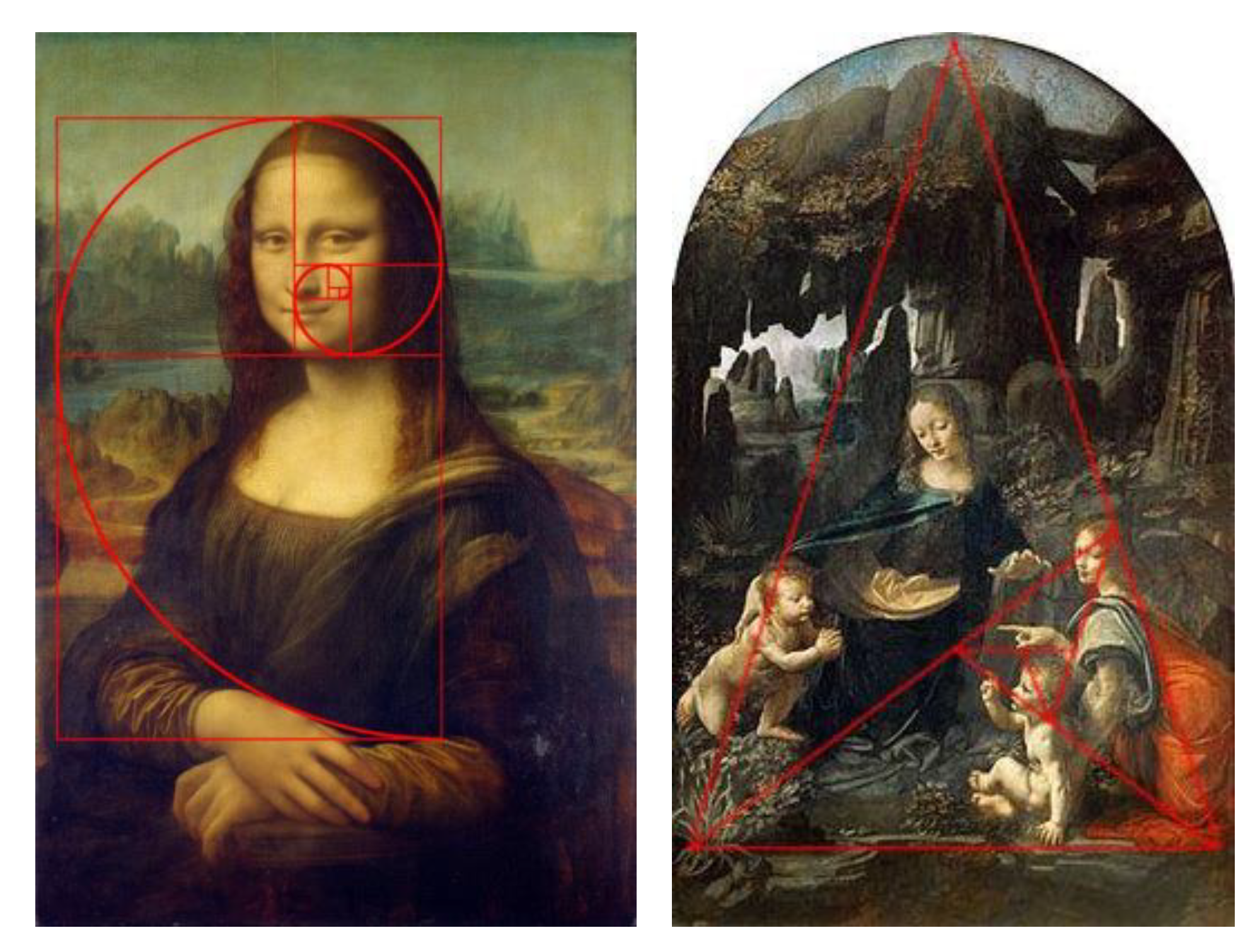
Figure 3.
Benchmark of image analysis: (a) White noise; (b) Image with clustering; (c) Art painting. The lower row depicts the average brightness in the upper one.
Figure 3.
Benchmark of image analysis: (a) White noise; (b) Image with clustering; (c) Art painting. The lower row depicts the average brightness in the upper one.

Figure 4.
Example of stochastic analysis of 2D picture, in escalating spatial scales. Grouped pixels at different scales are used to calculate the climacogram: (a) White noise; (b) Image with clustering; (c) Art painting.
Figure 4.
Example of stochastic analysis of 2D picture, in escalating spatial scales. Grouped pixels at different scales are used to calculate the climacogram: (a) White noise; (b) Image with clustering; (c) Art painting.

Figure 5.
(a) Climacograms of the benchmark images; (b) Standardized climacograms of the benchmark images.
Figure 5.
(a) Climacograms of the benchmark images; (b) Standardized climacograms of the benchmark images.

Figure 19.
Coefficient of variation of standard deviation over the average of Picasso’s and Da Vinci’s artworks’ climacograms.
Figure 19.
Coefficient of variation of standard deviation over the average of Picasso’s and Da Vinci’s artworks’ climacograms.

Figure 20.
Leonardo da Vinci, Virgin of the Rocks. (a) Louvre version, 1483–1486; (b) National Gallery of London, before 1508.
Figure 20.
Leonardo da Vinci, Virgin of the Rocks. (a) Louvre version, 1483–1486; (b) National Gallery of London, before 1508.

© 2020 by the authors. Licensee MDPI, Basel, Switzerland. This article is an open access article distributed under the terms and conditions of the Creative Commons Attribution (CC BY) license (http://creativecommons.org/licenses/by/4.0/).
Share and Cite
MDPI and ACS Style
Sargentis, G.-F.; Dimitriadis, P.; Koutsoyiannis, D. Aesthetical Issues of Leonardo Da Vinci’s and Pablo Picasso’s Paintings with Stochastic Evaluation. Heritage 2020, 3, 283-305. https://0-doi-org.brum.beds.ac.uk/10.3390/heritage3020017
AMA Style
Sargentis G-F, Dimitriadis P, Koutsoyiannis D. Aesthetical Issues of Leonardo Da Vinci’s and Pablo Picasso’s Paintings with Stochastic Evaluation. Heritage. 2020; 3(2):283-305. https://0-doi-org.brum.beds.ac.uk/10.3390/heritage3020017
Chicago/Turabian StyleSargentis, G.-Fivos, Panayiotis Dimitriadis, and Demetris Koutsoyiannis. 2020. "Aesthetical Issues of Leonardo Da Vinci’s and Pablo Picasso’s Paintings with Stochastic Evaluation" Heritage 3, no. 2: 283-305. https://0-doi-org.brum.beds.ac.uk/10.3390/heritage3020017