On-Site VIS-NIR Spectral Reflectance and Colour Measurements—A Fast and Inexpensive Alternative for Delineating Sediment Layers Quantitatively? A Case Study from a Monumental Bronze Age Burial Mound (Seddin, Germany)


Abstract
:
1. Introduction
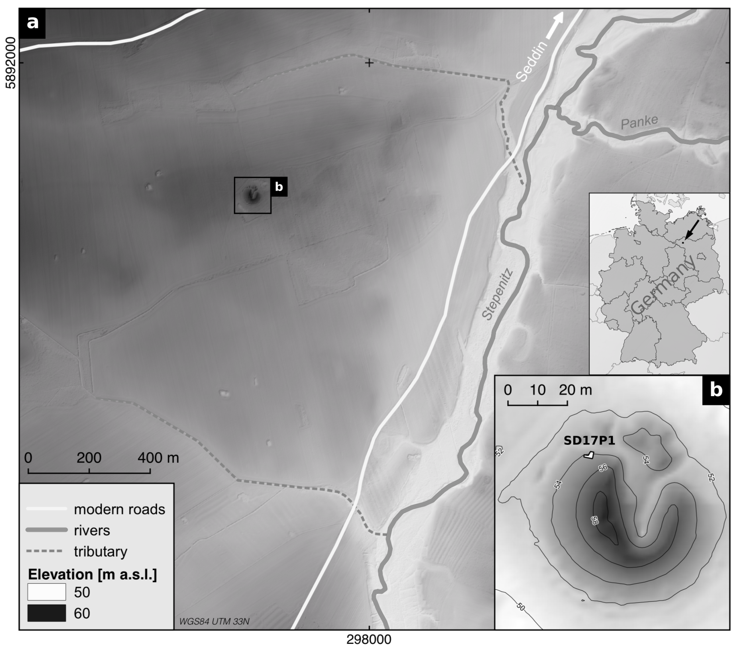
Study Site
2. Materials and Methods
2.1. Laboratory Sediment Analyses
2.1.1. Water Content
2.1.2. Soil Organic Carbon
2.1.3. pH Value
2.1.4. Grain Size
2.1.5. Element Concentrations
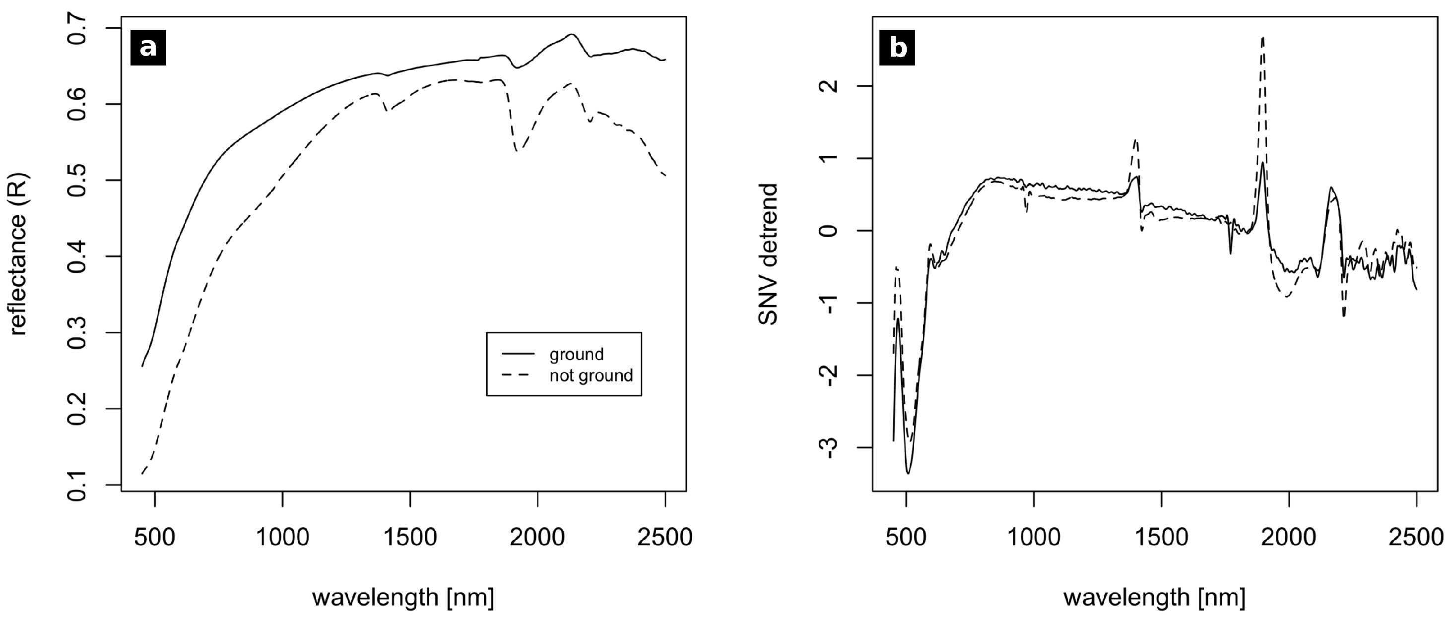
2.1.6. Visible and Near-Infrared Spectroscopy
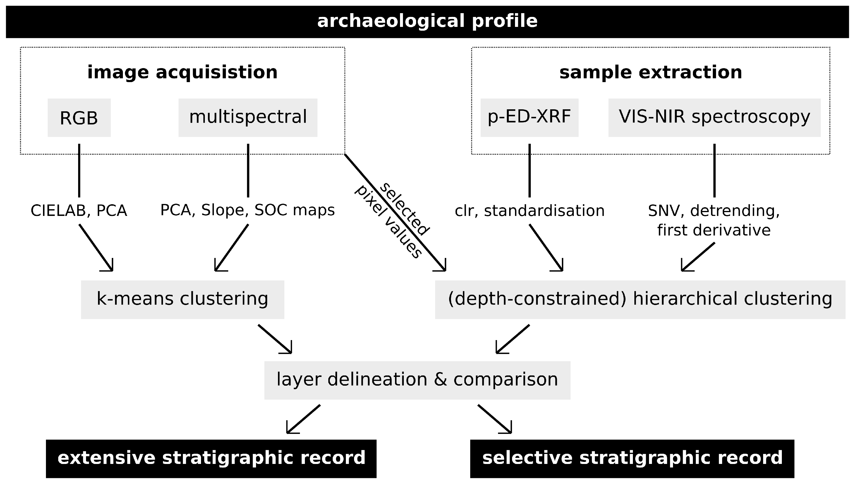
2.2. Image Acquisition
2.3. Image Analysis
2.3.1. Image Pre-Processing
2.3.2. Slope Rasters
2.3.3. Principal Component Analysis
2.3.4. CIELAB
2.3.5. Soil Organic Carbon
2.4. Cluster Analysis
2.4.1. Sedimentological Data
2.4.2. Image Data
3. Results
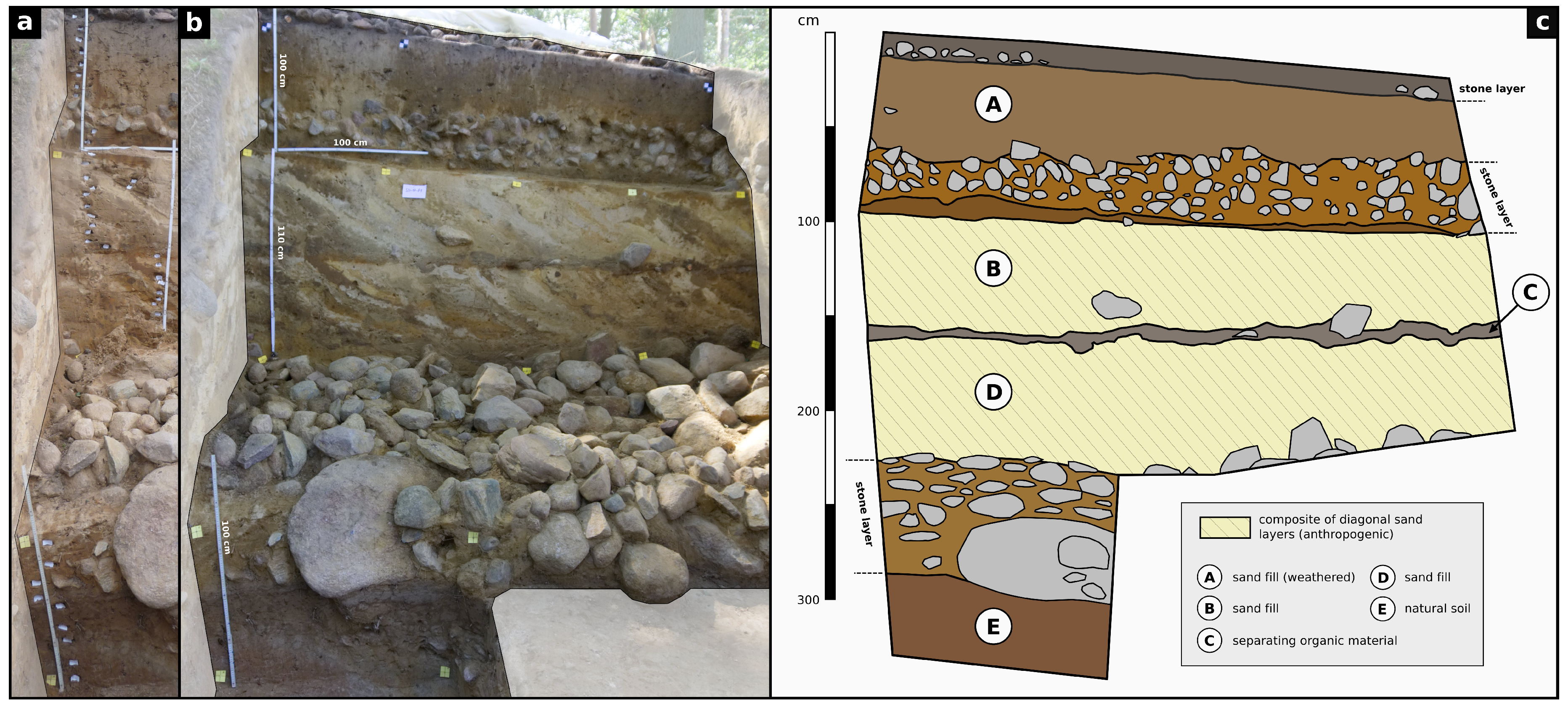
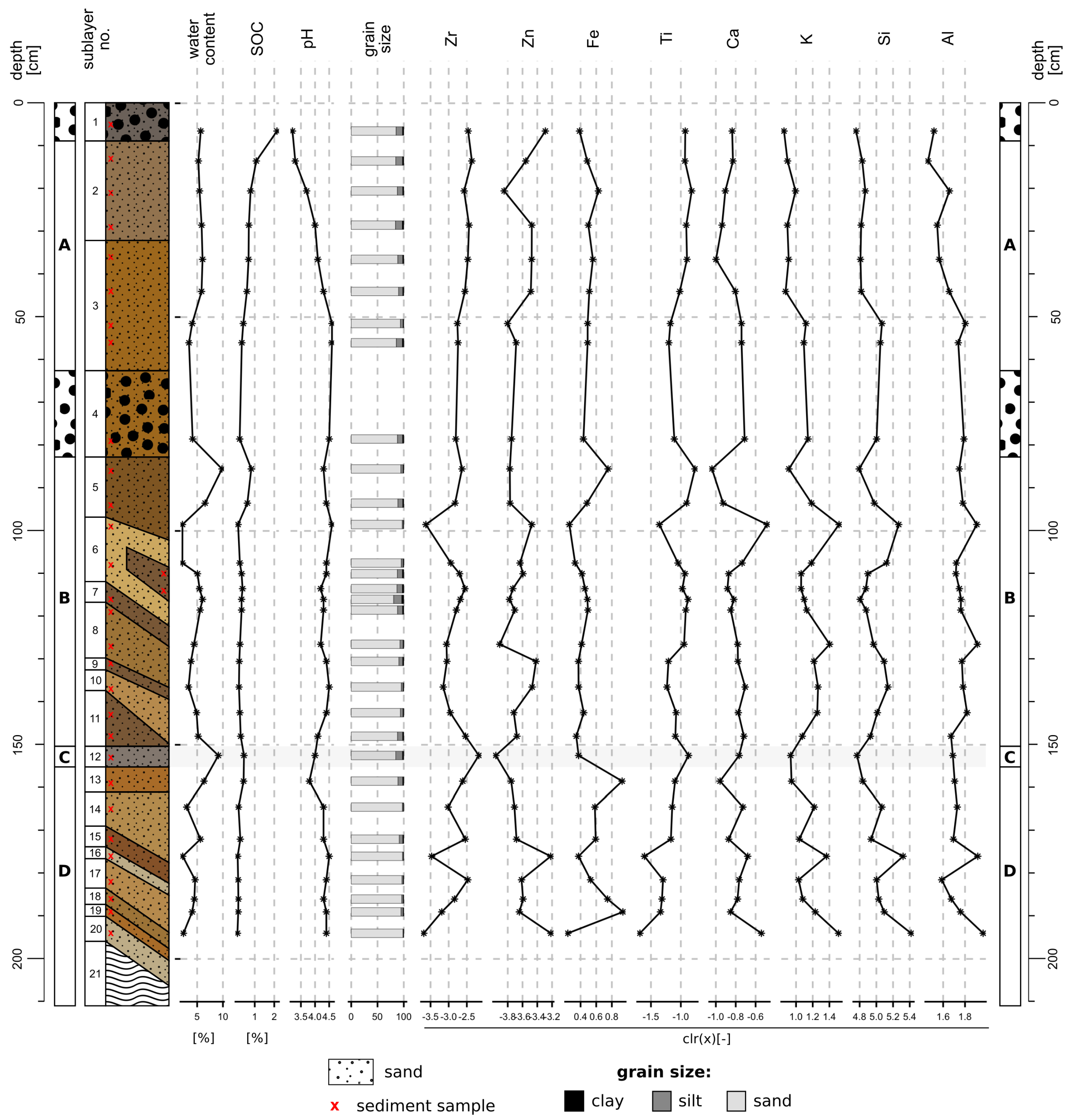
3.1. Sedimentological Record
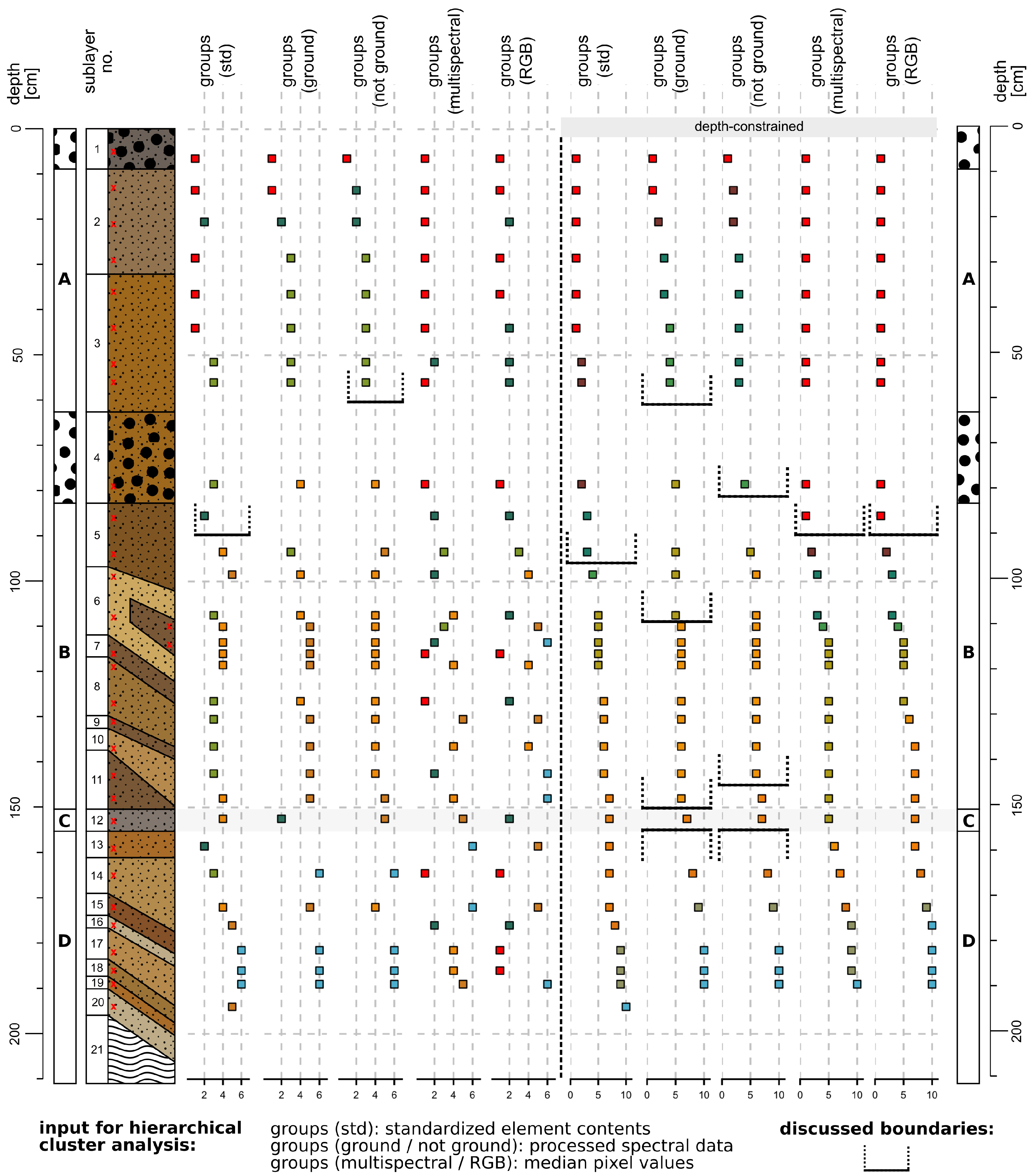
3.2. Clustering Results—Sedimentological Data
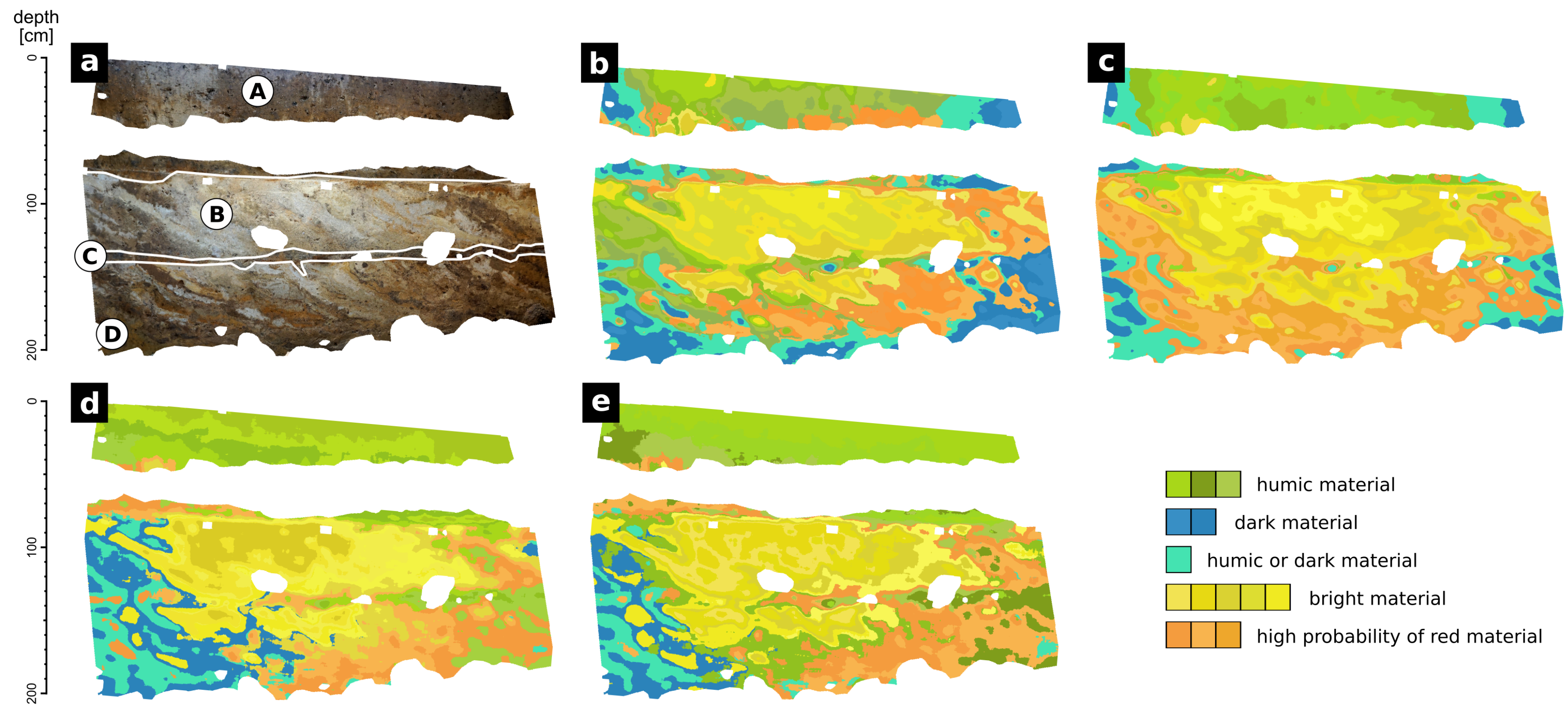
3.3. Clustering Results—Image Data
4. Discussion
4.1. Image Data
4.2. Sedimentological Data
4.3. Shortcomings and Benefits of Spectral Measurements
5. Conclusions
Supplementary Materials
Author Contributions
Funding
Acknowledgments
Conflicts of Interest
Abbreviations
| VIS-NIR | visible and near-infrared |
| SOC | soil organic carbon |
| p-ED-XRF | portable energy-dispersive X-ray fluorescence spectrometer |
| CRM | certified reference material |
| SNV | standard normal variate |
| clr | centred log ratio |
| TPS | thin plate spline |
| FWHM | full width half maximum |
| PCA | principle component analysis |
References
- Harris, E.C. Principles of Archaeological Stratigraphy; Academic Press: London, UK, 1979. [Google Scholar]
- Vincent, M.L.; Kuester, F.; Levy, T.E. Opendig: Contextualizing the past from the field to the web. Mediterr. Archaeol. Archaeom. 2014, 14, 109–116. [Google Scholar]
- Simonson, R.W. Soil Color Standards and Terms for Field Use—History of Their Development. Soil Color 1993, 31, 1–20. [Google Scholar] [CrossRef]
- Landa, E.R.; Fairchild, M.D. Charting Color from the Eye of the Beholder. Am. Sci. 2005, 93, 436–443. [Google Scholar] [CrossRef]
- Hassan, F.A. Sediments in Archaeology: Methods and Implications for Palaeoenvironmental and Cultural Analysis. J. Field Archaeol. 1978, 5, 197–213. [Google Scholar] [CrossRef]
- Goldberg, P.; Holliday, V.T.; Ferring, C.R. Earth Sciences and Archaeology; Springer Science & Business Media: New York, NY, USA, 2013. [Google Scholar]
- Hoelzmann, P.; Klein, T.; Kutz, F.; Schütt, B. A new device to mount portable energy-dispersive X-ray fluorescence spectrometers (p-ED-XRF) for semi-continuous analyses of split (sediment) cores and solid samples. Geosci. Instrum. Methods Data Syst. 2017, 6, 93. [Google Scholar] [CrossRef] [Green Version]
- French, C. Geoarchaeology in Action: Studies in Soil Micromorphology and Landscape Evolution; Routledge: London, UK, 2003. [Google Scholar]
- Kooistra, M.J.; Kooistra, L.I. Integrated research in archaeology using soil micromorphology and palynology. CATENA 2003, 54, 603–617. [Google Scholar] [CrossRef]
- Meister, J.; Krause, J.; Müller-Neuhof, B.; Portillo, M.; Reimann, T.; Schütt, B. Desert agricultural systems at EBA Jawa (Jordan): Integrating archaeological and paleoenvironmental records. Quat. Int. 2017, 434, 33–50. [Google Scholar] [CrossRef]
- Zhang, Y.; Hartemink, A.E. A method for automated soil horizon delineation using digital images. Geoderma 2019, 343, 97–115. [Google Scholar] [CrossRef]
- Haburaj, V.; Krause, J.; Pless, S.; Waske, B.; Schütt, B. Evaluating the Potential of Semi-Automated Image Analysis for Delimiting Soil and Sediment Layers. J. Field Archaeol. 2019, 44. [Google Scholar] [CrossRef]
- Stenberg, B.; Viscarra Rossel, R.A. Diffuse Reflectance Spectroscopy for High-Resolution Soil Sensing. In Proximal Soil Sensing; Viscarra Rossel, R.A., McBratney, A.B., Minasny, B., Eds.; Progress in Soil Science; Springer: Dordrecht, The Netherlands, 2010; pp. 29–47. [Google Scholar] [CrossRef]
- Debret, M.; Sebag, D.; Desmet, M.; Balsam, W.; Copard, Y.; Mourier, B.; Susperrigui, A.S.; Arnaud, F.; Bentaleb, I.; Chapron, E.; et al. Spectrocolorimetric interpretation of sedimentary dynamics: The new “Q7/4 diagram”. Earth-Sci. Rev. 2011, 109, 1–19. [Google Scholar] [CrossRef] [Green Version]
- Zeeden, C.; Krauß, L.; Kels, H.; Lehmkuhl, F. Digital image analysis of outcropping sediments: Comparison to photospectrometric data from Quaternary loess deposits at Şanoviţa (Romania) and Achenheim (France). Quat. Int. 2017, 429, 100–107. [Google Scholar] [CrossRef]
- Udelhoven, T.; Emmerling, C.; Jarmer, T. Quantitative analysis of soil chemical properties with diffuse reflectance spectrometry and partial least-square regression: A feasibility study. Plant Soil 2003, 251, 319–329. [Google Scholar] [CrossRef]
- Mutuo, P.K.; Shepherd, K.D.; Albrecht, A.; Cadisch, G. Prediction of carbon mineralization rates from different soil physical fractions using diffuse reflectance spectroscopy. Soil Biol. Biochem. 2006, 38, 1658–1664. [Google Scholar] [CrossRef]
- Brown, D.J.; Shepherd, K.D.; Walsh, M.G.; Dewayne Mays, M.; Reinsch, T.G. Global soil characterization with VNIR diffuse reflectance spectroscopy. Geoderma 2006, 132, 273–290. [Google Scholar] [CrossRef]
- Sankey, J.B.; Brown, D.J.; Bernard, M.L.; Lawrence, R.L. Comparing local vs. global visible and near-infrared (VisNIR) diffuse reflectance spectroscopy (DRS) calibrations for the prediction of soil clay, organic C and inorganic C. Geoderma 2008, 148, 149–158. [Google Scholar] [CrossRef] [Green Version]
- Volkan Bilgili, A.; van Es, H.M.; Akbas, F.; Durak, A.; Hively, W.D. Visible-near infrared reflectance spectroscopy for assessment of soil properties in a semi-arid area of Turkey. J. Arid Environ. 2010, 74, 229–238. [Google Scholar] [CrossRef]
- Soriano-Disla, J.M.; Janik, L.J.; Viscarra Rossel, R.A.; Macdonald, L.M.; McLaughlin, M.J. The Performance of Visible, Near-, and Mid-Infrared Reflectance Spectroscopy for Prediction of Soil Physical, Chemical, and Biological Properties. Appl. Spectrosc. Rev. 2014, 49, 139–186. [Google Scholar] [CrossRef]
- Melville, M.D.; Atkinson, G. Soil colour: Its measurement and its designation in models of uniform colour space. J. Soil Sci. 1985, 36, 495–512. [Google Scholar] [CrossRef]
- Viscarra Rossel, R.A.; Walvoort, D.J.J.; McBratney, A.B.; Janik, L.J.; Skjemstad, J.O. Visible, near infrared, mid infrared or combined diffuse reflectance spectroscopy for simultaneous assessment of various soil properties. Geoderma 2006, 131, 59–75. [Google Scholar] [CrossRef]
- Jarmer, T.; Lavée, H.; Hill, P.S.J. Using Reflectance Spectroscopy and Landsat Data to Assess Soil Inorganic Carbon in the Judean Desert (Israel). In Recent Advances in Remote Sensing and Geoinformation Processing for Land Degradation Assessment; Röder, A., Hill, J., Eds.; CRC Press: London, UK, 2009; pp. 227–243. [Google Scholar] [CrossRef]
- Hill, J.; Udelhoven, T.; Vohland, M.; Stevens, A. The Use of Laboratory Spectroscopy and Optical Remote Sensing for Estimating Soil Properties. In Precision Crop Protection—The Challenge and Use of Heterogeneity; Oerke, E.C., Gerhards, R., Menz, G., Sikora, R.A., Eds.; Springer: Dordrecht, The Netherlands, 2010; pp. 67–85. [Google Scholar] [CrossRef]
- Sprafke, T. Löss in Niederösterreich—Archiv Quartärer Klima- und Landschaftsveränderungen; Würzburg University Press: Würzburg, Germany, 2016. [Google Scholar]
- Vodyanitskii, Y.N.; Kirillova, N.P. Application of the CIE-L*a*b* system to characterize soil color. Eurasian Soil Sci. 2016, 49, 1259–1268. [Google Scholar] [CrossRef]
- Zhang, Y.; Hartemink, A.E. Digital mapping of a soil profile. Eur. J. Soil Sci. 2019, 70, 27–41. [Google Scholar] [CrossRef] [Green Version]
- Kiekebusch, A. Das Königsgrab von Seddin. In Führer zur Urgeschichte; Number 1; Dt. Buchvertr. Ges.: Augsburg, Germany, 1928. [Google Scholar]
- May, J. Der Fundplatz und die Umgebung des Grabhügels von Seddin als ortsfestes Bodendenkmal. In Jürgen Kunow (Hrsg.), Das »Königsgrab« von Seddin in der Prignitz. Kolloquium Anlässlich des 100. Jahrestages Seiner Freilegung am 12. Oktober 1999; Number 9 in Arbeitsberichte zur Bodendenkmalpflege in Brandenburg; Brandenburgisches Landesamt für Denkmalpflege und Archoläogisches Landesmuseum: Zossen, Germany, 2003; pp. 7–11. [Google Scholar]
- May, J.; Hauptmann, T. Das» Königsgrab «von Seddin und sein engeres Umfeld im Spiegel neuer Feldforschungen. In Gräberlandschaften der Bronzezeit. Internationales Kolloquium zur Bronzezeit; Bérenger, D., Bourgeois, J., Talon, M., St. Wirth (Hrsg.), Eds.; Number 51 in Bodenaltertümer Westfalens; LWL-Archäologie in Westfalen und Altertumskommission für Westfalen: Darmstadt, Germany, 2012. [Google Scholar]
- Wüstemann, H. Zur Sozialstruktur im Seddiner Kulturgebiet. Zeitschrift für Archäologie 1974, 8, 67–107. [Google Scholar]
- May, J. Neue Forschung am ’Königsgrab’ von Seddin. In Der Grabhügel von Seddin im Norddeutschen und Südskandinavischen Kontext; Hansen, S., Schopper, F., Eds.; Number 33 in Arbeitsberichte zur Bodendenkmalpflege in Brandenburg; Brandenburgisches Landesamt für Denkmalpflege und Archäologisches Landesmuseum: Zossen, Germany, 2018. [Google Scholar]
- Schenk, T.; Goldmann, T.; Kultfeuerreihe, D.S. Geomagnetische Prospektion am Königsgrab in der Prignitz. Arch. Berl. Brandenbg. 2003, 57–59. [Google Scholar]
- May, J. Fokussieren, Positionieren, Schritthalten. Aspekte von Raum und Zeit am ’Königsgrab’ von Seddin in der Prignitz. In Das Ganze Ist Mehr als die Summe Seiner Teile. Festschrift für Jürgen Kunow; Number 27 in Materialien zur Bodendenkmalpflege im Rheinland; LVR-Amt für Bodendenkmalpflege im Rheinland: Bonn, Germany, 2018. [Google Scholar]
- Landesamt für Bergbau, G.U.R. Geologische Karte 1:25.000 (GK25) des Landes Brandenburg, Blatt Baek (2837). 1905. Available online: https://lbgr.brandenburg.de/sixcms/detail.php/622447 (accessed on 15 June 2020).
- Götze, A. Die vor- und frühgeschichtlichen Denkmäler des Kreises Westprignitz. Kunstdenkmäler der Prov. Brandenbg. 1912, 1, 1–54. [Google Scholar]
- Brunke, H.; Bukowiecki, E.; Cancik-Kirschbaum, E.; Eichmann, R.; Ess, M.V.; Gass, A.; Gussone, M.; Hageneuer, S.; Hansen, S.; Kogge, W.; et al. Thinking Big. Research in Monumental Constructions in Antiquity. Space Knowl. 2016, 250–305. [Google Scholar] [CrossRef]
- Company, M.C. Munsell Soil Color Charts, Revised Edition; Munsell Color: Baltimore, Germany, 1994. [Google Scholar]
- Ad-hoc-Arbeitsgruppe Boden. Bodenkundliche Kartieranleitung (KA5), 5th ed.; Schweizerbart: Hannover, Germany, 2005. [Google Scholar]
- Blume, H.P.; Stahr, K.; Leinweber, P. Bodenkundliches Praktikum: Eine Einführung in Pedologisches Arbeiten für Ökologen, Land- und Forstwirte, Geo- und Umweltwissenschaftler; Springer: Heidelberg, Germany, 2011. [Google Scholar]
- Vogel, S.; Märker, M.; Rellini, I.; Hoelzmann, P.; Wulf, S.; Robinson, M.; Steinhübel, L.; Di Maio, G.; Imperatore, C.; Kastenmeier, P.; et al. From a stratigraphic sequence to a landscape evolution model: Late Pleistocene and Holocene volcanism, soil formation and land use in the shade of Mount Vesuvius (Italy). Quat. Int. 2016, 394, 155–179. [Google Scholar] [CrossRef]
- Schmidt, M.; Leipe, C.; Becker, F.; Goslar, T.; Hoelzmann, P.; Mingram, J.; Müller, S.; Tjallingii, R.; Wagner, M.; Tarasov, P.E. A multi-proxy palaeolimnological record of the last 16,600 years from coastal Lake Kushu in northern Japan. Palaeogeogr. Palaeoclimatol. Palaeoecol. 2019, 514, 613–626. [Google Scholar] [CrossRef]
- Aitchison, J. The Statistical Analysis of Compositional Data; Monographs on Statistics and Applied Probability; Chapman & Hall Ltd.: London, UK, 1986. [Google Scholar]
- R Core Team. R: A Language and Environment for Statistical Computing; R Foundation for Statistical Computing: Vienna, Austria, 2018. [Google Scholar]
- Boogaart, K.G.V.; Tolosana-Delgado, R.; Bren, M. Compositions: Compositional Data Analysis. 2018. Available online: https://cran.r-project.org/package=compositions (accessed on 15 June 2020).
- Sánchez-Marañón, M.; Delgado, G.; Delgado, R.; Pérez, M.M.; Melgosa, M. Spectroradiometric and visual color measurements of disturbed and undisturbed soil samples. Soil Sci. 1995, 160, 291–303. [Google Scholar] [CrossRef]
- Savitzky, A.; Golay, M.J.E. Smoothing and Differentiation of Data by Simplified Least Squares Procedures. Anal. Chem. 1964, 36, 1627–1639. [Google Scholar] [CrossRef]
- Lehnert, L.W.; Meyer, H.; Bendix, J. HSDAR: Manage, Analyse and Simulate Hyperspectral Data in R; 2017; Available online: https://cran.r-project.org/package=hsdar (accessed on 15 June 2020).
- Stenberg, B.; Viscarra Rossel, R.A.; Mouazen, A.M.; Wetterlind, J. Visible and Near Infrared Spectroscopy in Soil Science. In Advances in Agronomy; Sparks, D.L., Ed.; Academic Press: Burlington, MA, USA, 2010; Volume 107, pp. 163–215. [Google Scholar] [CrossRef] [Green Version]
- Owen, A.J. Uses of derivative spectroscopy. Agil. Technol. 1995, 8. [Google Scholar]
- Barnes, R.J.; Dhanoa, M.S.; Lister, S.J. Standard Normal Variate Transformation and De-trending of Near-Infrared Diffuse Reflectance Spectra. Appl. Spectrosc. 1989, 43, 772–777. [Google Scholar] [CrossRef]
- Retzlaff, R. On the Potential of Small UAS for Multispectral Remote Sensing in Large-Scale Agricultural and Archaeological Applications. Ph.D. Thesis, Universität Trier, Trier, Germany, 2015. [Google Scholar]
- Duchon, J. Splines minimizing rotation-invariant semi-norms in Sobolev spaces. In Constructive Theory of Functions of Several Variables; Lecture Notes in Mathematics; Springer: Berlin/Heidelberg, Germany, 1977; pp. 85–100. [Google Scholar] [CrossRef]
- Hijmans, R.J. Raster: Geographic Data Analysis and Modeling. 2019. Available online: https://cran.r-project.org/package=raster (accessed on 15 June 2020).
- Leutner, B.; Horning, N. RStoolbox: Tools for Remote Sensing Data Analysis. 2017. Available online: https://cran.r-project.org/package=RStoolbox (accessed on 15 June 2020).
- Jarmer, T.; Schütt, B. Analysis of iron contents in carbonate bedrock by spectroradiometric detection based on experimentally designed substrates. In 1st EARSeL Workshop on Imaging Spectroscopy; Remote Sensing Laboratories, University of Zurich: Zurich, Switzerland, 1998; pp. 375–382. [Google Scholar]
- Schwertmann, U.; Cornell, R.M. Iron Oxides in the Laboratory: Preparation and Characterization; John Wiley & Sons: Weinheim, Germany, 2008. [Google Scholar]
- Barron, V.; Torrent, J. Use of the Kubelka—Munk theory to study the influence of iron oxides on soil colour. J. Soil Sci. 1986, 37, 499–510. [Google Scholar] [CrossRef]
- Baumgardner, M.; Silva, L.; Biehl, L.; Stoner, E. Reflectance properties of soils. Adv. Agron. 1985, 38, 1–44. [Google Scholar]
- Hill, J.; Schütt, B. Mapping Complex Patterns of Erosion and Stability in Dry Mediterranean Ecosystems. Remote Sens. Environ. 2000, 74, 557–569. [Google Scholar] [CrossRef]
- Steffens, M.; Kohlpaintner, M.; Buddenbaum, H. Fine spatial resolution mapping of soil organic matter quality in a Histosol profile. Eur. J. Soil Sci. 2014, 65, 827–839. [Google Scholar] [CrossRef]
- Hobley, E.; Steffens, M.; Bauke, S.; Kögel-Knabner, I. Hotspots of soil organic carbon storage revealed by laboratory hyperspectral imaging. Sci. Rep. 2018, 8. [Google Scholar] [CrossRef]
- Strauss, T.; Maltitz, M.J.v. Generalising Ward’s Method for Use with Manhattan Distances. PLoS ONE 2017, 12, e0168288. [Google Scholar] [CrossRef] [Green Version]
- Gill, D.; Shomrony, A.; Fligelman, H. Numerical Zonation of Log Suites and Logfacies Recognition by Multivariate Clustering. AAPG Bull. 1993, 77, 1781–1791. [Google Scholar]
- Grimm, E.C. CONISS: A FORTRAN 77 program for stratigraphically constrained cluster analysis by the method of incremental sum of squares. Comput. Geosci. 1987, 13, 13–35. [Google Scholar] [CrossRef]
- Hartigan, J.A.; Wong, M.A. Algorithm AS 136: A k-means clustering algorithm. J. R. Stat. Soc. Ser. C (Appl. Stat.) 1979, 28, 100–108. [Google Scholar] [CrossRef]
- Hornik, K. A CLUE for CLUster Ensembles. J. Stat. Softw. 2005, 14. [Google Scholar] [CrossRef]
- Schoeneberger, P.; Wysocki, D.; Benham, E.; Staff, S.S. Field Book for Describing and Sampling Soils; Version 3.0.; Natural Resources Conservation Service, National Soil Survey Center: Lincoln, NE, USA, 2012.
- Zhang, Y.; Hartemink, A.E. Soil horizon delineation using vis-NIR and pXRF data. Catena 2019, 180, 298–308. [Google Scholar] [CrossRef]
- Daniel, K.W.; Tripathi, N.K.; Honda, K. Artificial neural network analysis of laboratory and in situ spectra for the estimation of macronutrients in soils of Lop Buri (Thailand). Soil Res. 2003, 41, 47–59. [Google Scholar] [CrossRef]
- Viscarra Rossel, R.A.; Behrens, T. Using data mining to model and interpret soil diffuse reflectance spectra. Geoderma 2010, 158, 46–54. [Google Scholar] [CrossRef]
- Morellos, A.; Pantazi, X.E.; Moshou, D.; Alexandridis, T.; Whetton, R.; Tziotzios, G.; Wiebensohn, J.; Bill, R.; Mouazen, A.M. Machine learning based prediction of soil total nitrogen, organic carbon and moisture content by using VIS-NIR spectroscopy. Biosyst. Eng. 2016, 152, 104–116. [Google Scholar] [CrossRef] [Green Version]
- Viscarra Rossel, R.A.; Cattle, S.R.; Ortega, A.; Fouad, Y. In situ measurements of soil colour, mineral composition and clay content by vis–NIR spectroscopy. Geoderma 2009, 150, 253–266. [Google Scholar] [CrossRef]
- Post, J.L.; Noble, P.N. The Near-Infrared Combination Band Frequencies of Dioctahedral Smectites, Micas, and Illites. Clays Clay Miner. 1993, 41, 639–644. [Google Scholar] [CrossRef]
- Bishop, J.L.; Pieters, C.M.; Edwards, J.O. Infrared Spectroscopic Analyses on the Nature of Water in Montmorillonite. Clays Clay Miner. 1994, 42, 702–716. [Google Scholar] [CrossRef]
- Madejova, J.; Komadel, P. Baseline studies of the clay minerals society source clays: Infrared methods. Clays Clay Miner. 2001, 49, 410–432. [Google Scholar] [CrossRef]
- Fairchild, M. Color Appearance Models; John Wiley & Sons: Chichester, UK, 2013. [Google Scholar]
- Liu, H.; Huang, M.; Cui, G.; Luo, M.; Melgosa, M. Color-difference evaluation for digital images using a categorical judgment method. J. Opt. Soc. Am. A 2013, 30, 616–626. [Google Scholar] [CrossRef]
- Sánchez-Marañón, M.; García, P.; Huertas, R.; Hernández-Andrés, J.; Melgosa, M. Influence of Natural Daylight on Soil Color Description: Assessment Using a Color-Appearance Model. Soil Sci. Soc. Am. J. 2011, 75, 984–993. [Google Scholar] [CrossRef]
- Funt, B.; Bastani, P. Irradiance-independent camera color calibration. Color Res. Appl. 2014, 39, 540–548. [Google Scholar] [CrossRef]
- Bareth, G.; Aasen, H.; Bendig, J.; Gnyp, M.L.; Bolten, A.; Jung, A.; Michels, R.; Soukkamäki, J. Low-weight and UAV-based Hyperspectral Full-frame Cameras for Monitoring Crops: Spectral Comparison with Portable Spectroradiometer Measurements. Photogramm. Fernerkund. Geoinf. 2015, 2015, 69–79. [Google Scholar] [CrossRef]
- Behmann, J.; Acebron, K.; Emin, D.; Bennertz, S.; Matsubara, S.; Thomas, S.; Bohnenkamp, D.; Kuska, M.T.; Jussila, J.; Salo, H.; et al. Specim IQ: Evaluation of a New, Miniaturized Handheld Hyperspectral Camera and Its Application for Plant Phenotyping and Disease Detection. Sensors 2018, 18, 441. [Google Scholar] [CrossRef] [PubMed] [Green Version]
- Lodhi, V.; Chakravarty, D.; Mitra, P. Hyperspectral Imaging for Earth Observation: Platforms and Instruments. J. Indian Inst. Sci. 2018, 98, 429–443. [Google Scholar] [CrossRef]


| Sony ILCE-6000 | TetraCAM MicroMCA-6 | |
|---|---|---|
| B | 485 nm | 490 nm |
| G | 540 nm | 550 nm |
| R | 595 nm | 680 nm |
| red edge | - | 720 nm |
| NIR1 | - | 800 nm |
| NIR2 | - | 900 nm |
| spatial resolution | 5696 × 4272 px | 1280 × 1024 px |
| colour depth | 8 bit | 10 bit |
© 2020 by the authors. Licensee MDPI, Basel, Switzerland. This article is an open access article distributed under the terms and conditions of the Creative Commons Attribution (CC BY) license (http://creativecommons.org/licenses/by/4.0/).
Share and Cite
Haburaj, V.; Nykamp, M.; May, J.; Hoelzmann, P.; Schütt, B. On-Site VIS-NIR Spectral Reflectance and Colour Measurements—A Fast and Inexpensive Alternative for Delineating Sediment Layers Quantitatively? A Case Study from a Monumental Bronze Age Burial Mound (Seddin, Germany). Heritage 2020, 3, 528-548. https://0-doi-org.brum.beds.ac.uk/10.3390/heritage3020031
Haburaj V, Nykamp M, May J, Hoelzmann P, Schütt B. On-Site VIS-NIR Spectral Reflectance and Colour Measurements—A Fast and Inexpensive Alternative for Delineating Sediment Layers Quantitatively? A Case Study from a Monumental Bronze Age Burial Mound (Seddin, Germany). Heritage. 2020; 3(2):528-548. https://0-doi-org.brum.beds.ac.uk/10.3390/heritage3020031
Chicago/Turabian StyleHaburaj, Vincent, Moritz Nykamp, Jens May, Philipp Hoelzmann, and Brigitta Schütt. 2020. "On-Site VIS-NIR Spectral Reflectance and Colour Measurements—A Fast and Inexpensive Alternative for Delineating Sediment Layers Quantitatively? A Case Study from a Monumental Bronze Age Burial Mound (Seddin, Germany)" Heritage 3, no. 2: 528-548. https://0-doi-org.brum.beds.ac.uk/10.3390/heritage3020031