1. Introduction
The advent of the Finite Element Method (FEM) opened a new horizon for numerical simulation studies. In FEM, a physical phenomenon is described by a series of partial differential equations (PDEs) over an interested discretized domain or a series of domains. The PDEs are solved over each element of the discretization. Hence, the more appropriate is the discretization, the better approximation is the solution.
As in almost every field of science, corrosion science advances as a result of a mutual relationship between theory, experiment, and simulation [
1]. Nonetheless, corrosion modelers smartly have benefitted from FEM as it is able to provide more solution flexibility in terms of dealing with problem complexities [
2]. In addition, other numerical techniques exist for corrosion modeling such as finite difference method [
3], cellular automata [
4], finite volume method [
5], and boundary element method [
6], to which interested readers could refer to; the provided references are not meant to be complete. Nevertheless, the focus of this perspective paper is only FEM for corrosion modeling.
Speaking of problem complexity in corrosion modelling studies, the case of atmospheric corrosion will be highlighted in more detail. In atmospheric corrosion studies, there is an extremely thin layer of electrolyte, meaning the domain has a high aspect ratio, which even changes over time due to evaporation/condensation, deliquesce properties of the aerosols, and relative humidity [
7]. Furthermore, the size of the electrodes changes due to corrosion or deposition of products, and the electrolyte chemistry changes as the species are consumed/produced, causing high concentration gradients in the electrolyte. FEM–at least in theory–is able to deal with such complexities.
In FEM simulations in corrosion science, there are two main approaches: (i) using the Nernst–Planck (NP) equation and (ii) using the Laplace equation. The NP equation depicts the transport of species in the electrolyte as a summation of diffusion, migration, and convection:
where,
Ji,
Di,
ci,
zi,
ui,
F,
φ, and
v are the flux, diffusion coefficient, concentration, charge, mobility, Faraday constant, electric potential, and solution-velocity, respectively.
In addition, in the case of homogeneous chemical reactions between the species in the electrolyte, the production/consumption rate term
will be introduced:
Also, the current density in the electrolyte
is given as:
where Equation (3) combined with conservation of charge (
), yields:
from which the electrolyte current density can be obtained.
Therefore, the NP equation is regarded as the most complete means to solve transient problems in electrochemical systems, as it yields the concentration gradient, electrolyte current density, and electrolyte potential distribution.
However, the NP equation approach is computationally expensive as it takes into account the many parameters to solve. One alternative approach is to use the Laplace equation:
The Laplace equation approach depends on electrolyte conductivity, boundary conditions, etc. However, when the electrolyte resistance is not uniform, the Laplace equation approach would not be the most accurate approach.
Taking into account some of the highlighted recent advances in thin film corrosion FEM modelling, this paper aims at providing a perspective on not only how far the field has come, but also how far it still is from a complete thin film corrosion model, along with what needs to be included to advance the models further. Atmospheric corrosion modelling is taken for the base herein, as it is one of the best resemblances of thin film corrosion and in terms of modelling is one of the most complex forms of corrosion.
Thin film corrosion, or in general, atmospheric corrosion, is probably the most common form of corrosion. Almost all industrial and municipal sectors involve atmospheric corrosion directly, such as oil and gas, water and desalination, transportation, power plants, food and beverage, etc., destroying money and infrastructure. The mechanism of thin film corrosion is different than the bulk electrolyte corrosion mechanism and thin film corrosion rate highly depends on the electrolyte thickness. Altogether, it is of crucial importance to bring more insights to thin film corrosion mechanisms by mechanism modelling studies for better understanding, prediction, and implementation of corrosion management strategies.
It is worth noting that although this paper focuses on atmospheric corrosion as a complex form of thin film corrosion, it could still be applicable in other areas where a thin film of corrosive electrolyte condensates. For instance, internal corrosion of oil and gas pipelines—where the fluid is wet—or cooling systems such as cooling towers and heat exchangers or external corrosion of pipelines under disbonded coatings are all likely to occur under a thin layer of electrolyte [
8].
2. The Current Status of FEM Thin Film Corrosion Modelling: Where We Advanced?
Recently, Liu and Kelly [
9] published a holistic review on the application of FEM to modelling localized corrosion. Our paper is focused explicitly on FEM for thin film (and extremely thin film) corrosion, applicable to atmospheric corrosion, in a very concise and straightforward manner—taking into account only the highlighted works in this field and discussing them in a different perspective than in reference [
9]. In addition, an essential contribution in this field was on FEM moving boundary simulation [
10,
11] that was published after the review of Liu and Kelly, which is included here. Incorporation of the concept of a moving boundary in FEM corrosion modelling will be crucial for future research directions, as will be explained in
Section 3.
Simulation of atmospheric corrosion is a complex study as the electrolyte film evaporates and condenses cyclically, but without any known order in terms of rate and extent of these processes, due to the various environmental parameters that randomly affect condensation/evaporation. Under certain circumstances, while evaporating, the electrolyte film breaks into droplets, or even droplets could be present from the beginning. The effect of environmental parameters on spatial distribution, number, size, critical size, etc. of droplets are yet to be understood fully. Therefore, droplet corrosion modelling is out of the focus of this paper, despite the efforts that have so far been made on droplet corrosion modelling [
12]. Rather, corrosion modelling under thin
continuous electrolyte films is focused as this is where the majority of the previous work has been done and will eventually form the foundation for droplet corrosion modelling.
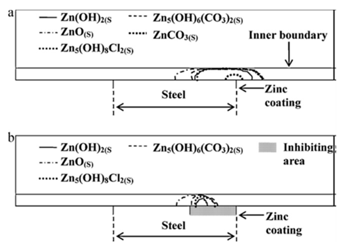
For the case of galvanic corrosion under constant thickness of electrolyte, in a series of works, Thébault et al. systematically studied galvanic corrosion between iron and zinc. They first started with a Laplace-Equation modelling approach [
13] in a 3000 µm thick electrolyte film domain and obtained good agreement between their model and scanning vibrating electrode measurements. Further, they applied an NP approach [
14] to include multiple species and reactions in the electrolyte film, which was divided into a 2500 µm bulk layer above a 500 µm diffusion layer, concluding that only the steel surface that was remote from the zinc coating was cathodically active with oxygen reduction being inhibited in the vicinity of the zinc due to presence of a dense layer of corrosion products. Also, Thébault et al. included five types of corrosion products deposition in their model: Zn(OH)
2(S), ZnO
(S), Zn
5(OH)
8Cl
2(S), Zn
5(OH)
6(CO
3)
2(S), ZnCO
3(S). However, due to the key drawback with their model, which was steady-state-formulation, was it could not take into account the accumulation of corrosion products. Rather, regions of the solution that were supersaturated with the corrosion products were predicted as depicted in
Figure 1. Likewise, Dolgikh et al. [
15] predicted corrosion products in a hot-dip galvanized Al(Zn, Mg) coating system.
The Laplacian approach for Fe-Zn galvanic corrosion was further developed by Thébault et al. [
16] to model galvanic corrosion under extremely thin electrolytes. They reported that the galvanic coupling was a function of the electrolyte thickness (from 1 cm to 1 µm). In their study, multiple coupling regimes were highlighted as the electrolyte thickness decreased, where the sacrificial protection mechanism changed from kinetic (cathodic) control under full immersion conditions, to ohmic control for very thin electrolyte films, leading to a decrease of the protection efficiency. However, as Thébault et al. used a Laplacian approach, their thin electrolyte model was not able to take into account concentration gradients and hence the conductivity within the thin electrolyte had to be taken as being uniform; which is not the most accurate assumption.
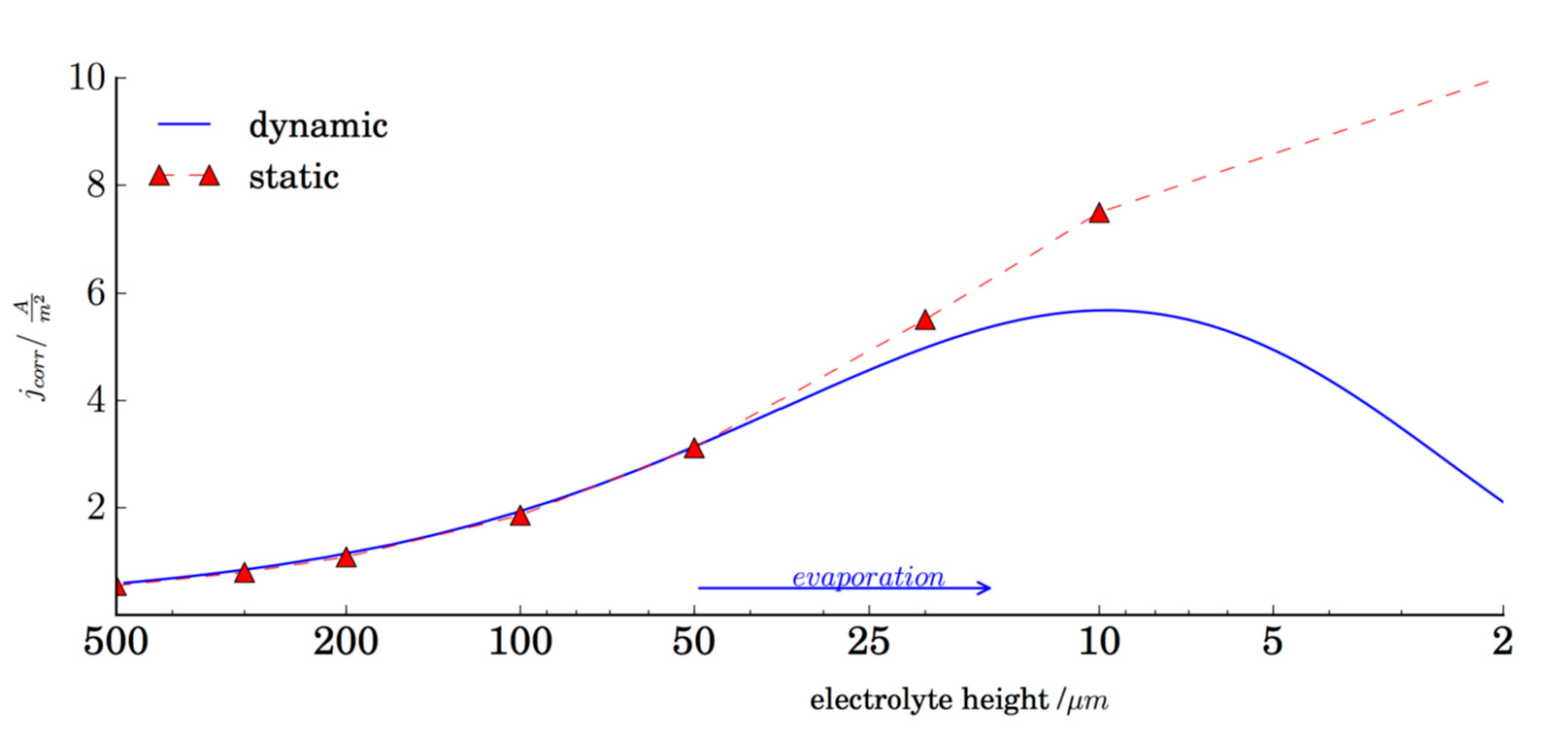
One of the key issues to be addressed is the simulation of a dynamic layer of varying thickness and concentrations due to evaporation, which can be done by the NP approach. This was addressed by Dolgikh et al. [
17], who started with a stagnant layer but found that the oxygen reduction reaction current deviated from Fick’s first law as the electrolyte thickness drops below 50–75 µm, due to increased ohmic resistance. However, for the dynamic layer, Dolgikh et al. found that the oxygen reduction reaction current was the result of two competing phenomena: reducing electrolyte thickness and increasing salt concentration leading to a decrease of oxygen solubility, where it first resulted in an increase in the oxygen reduction reaction current that peaked at an electrolyte thickness of 25 µm, at which point the second effect became dominant and the current dropped under thinner layers. By incorporating changes in ion diffusivity as a function of chloride concentration, Simillion et al. [
18] found that the peak current electrolyte thickness is reduced to 10 µm as depicted in
Figure 2. However, it should be noted that Simillion et al.’s study included far fewer species in the electrolyte compared to Thébault et al.’s [
14].
In the abovementioned models, the electrolyte thickness variation was not considered as being dependent of environmental parameters, which would be a more realistic case. To address this key point, van den Steen et al. [
8] developed a dynamic electrolyte film model for steel where the corrosion depended on the electrolyte thickness, the hygroscopic effect of salt, sample thickness, heat transfer, temperature change, and relative humidity. Even though van den Steen et al.’s work did not consider the changes in electrolyte chemistry caused by corrosion, a highlight output of their model was that the evaporation rate of electrolyte was not considered to be constant but instead determined by environmental parameters and physical parameters (such as heat conduction) of the steel electrode which is a more realistic case of electrolyte evaporation simulation. Later, Liu et al. [
19] modeled the total available cathodic current for stainless steel 316L galvanically coupled with aluminium alloy AA7050 as a function of electrolyte layer thickness as well as the length of the stainless steel. However, their work considered an unchanged solution concentration of constant conductivity, which reduces the applicability of the model for wet-dry cycles. In another work, Liu et al. [
20] modelled the corrosion damage prediction for galvanic coupling between a zinc plate and stainless-steel rods under a thin film electrolyte. However, the same assumption of constant electrolyte conductivity in one run of simulation was applied.
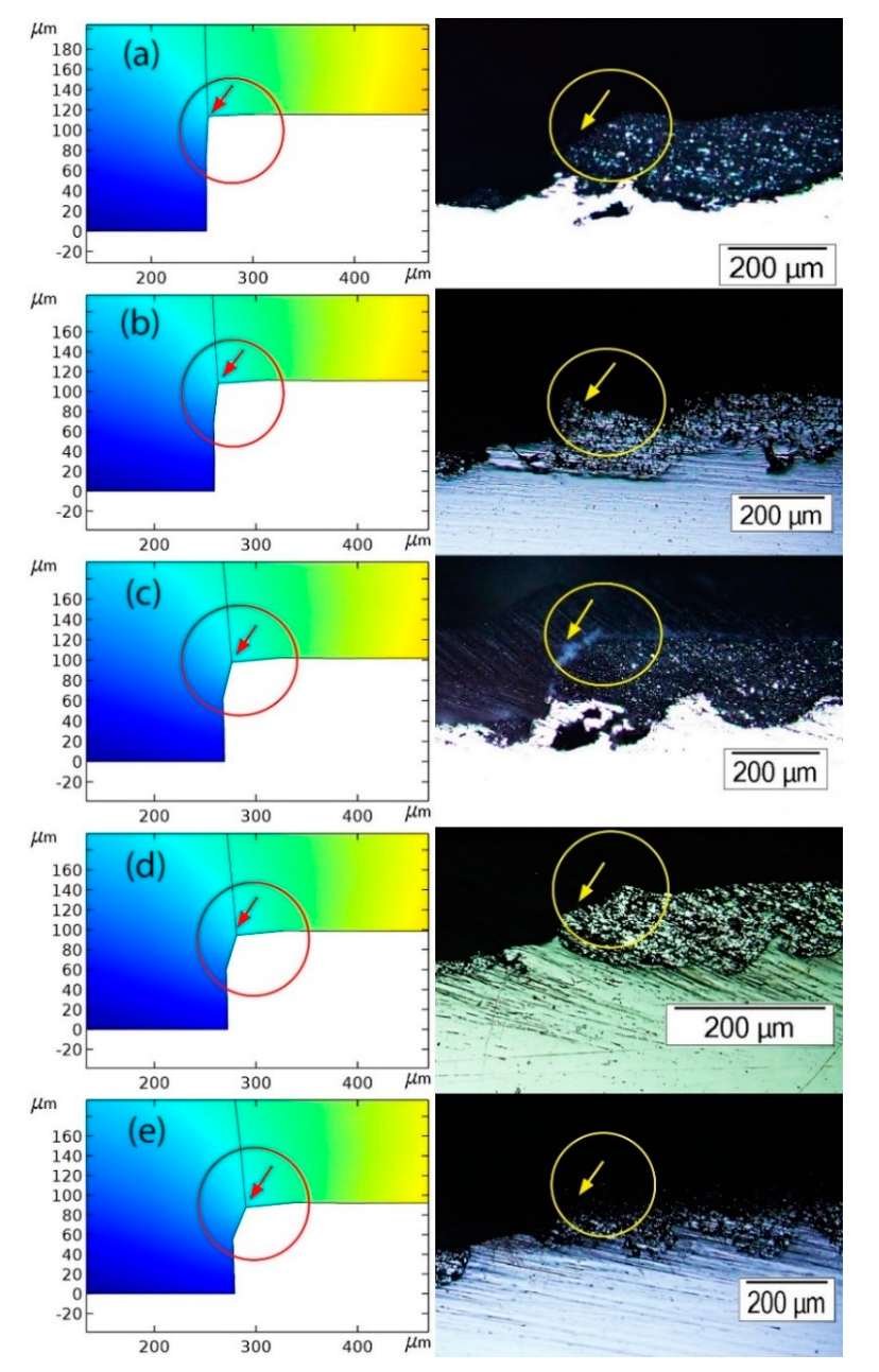
All of the simulation works above unanimously considered a constant size for the corroding electrode, rather than possibly the more accurate case of changing electrode size due to corrosion that would be obtained by a moving boundary simulation. Quite recently, Saeedikhani et al. [
10] developed a time-dependent, multi-species and multi-reaction moving boundary simulation for corrosion protection of an iron substrate provided by a scratched zinc coating. Their simulation showed that, while the middle of the scratch was protected by sacrificial protection, the corners of the scratch were under barrier protection, due to local cathodic inhibition arising from variations in the dissolved oxygen concentration over the surface of the scratched region. Moreover, the moving boundary simulation allowed the changes to the geometry of the corroding electrodes to be predicted. Finally, taking into account zinc electrodes consumption, the period of sacrificial protection was predicted. The introduction of the concept of moving boundary was of important progress in the field as nearly all the above-mentioned simulation studies considered a constant size for electrodes during corrosion, which is not the most accurate assumption.
Figure 3 shows a good agreement between the geometry of the actual corroded samples and simulation over corrosion exposure time.
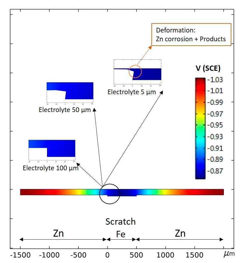
In addition, Saeedikhani et al. [
11] developed their simulation further to establish an iron-zinc sacrificial corrosion model under dynamic electrolyte thicknesses. In their thin film corrosion model, the electrode sizes change due to corrosion and precipitation of corrosion products was simulated as shown in
Figure 4. Also, the drying rate of the electrolyte was obtained by analyzing real-time corrosion monitoring data. Hence, the model is applicable to a simplified atmospheric corrosion condition. Their simulation results showed that the maximum corrosion rate occurs at an electrolyte thickness of about 8 µm, which is very close to the 10 µm value obtained by Simillion et al. [
18]. Moreover, the simulation of Saeedikhani et al. [
11] suggested that a cut-edge is a more severe defect than a scratch, with this being confirmed by the appearance of iron corrosion products on atmospheric exposed cut-edge samples whereas scratched samples were not corroded after one week of exposure. However, although their time-dependent model was able to depict the accumulation (growth) of a corrosion product layer, it considered Zn(OH)
2 as the only precipitating corrosion product. That is, other zinc corrosion products that are known to exist in the Fe-Zn galvanic corrosion system were not included [
21,
22].
3. The Future Needs and Prospects of FEM Thin Film Corrosion Modelling: Where We would Like to Advance?
Despite the many efforts so far, thin film corrosion modelers still strive to push the corrosion modelling edge further. The next step could be a thin film model that combines the work of Saeedikhani et al. [
11] and Van den Steen et al. [
8]. Not only would such a model be able to track the geometry change due to corrosion and product precipitation, but also allow the thickness of the thin film to change in response to variable environmental parameters; that is, evaporation/condensation would not be at constant rates. However, even after such an achievement, the following issues will remain outside the model, requiring further developments for their inclusion:
Electrode blockage due to corrosion products: Thébault et al. [
13] included an insulating (inactive) stick in their model to account for the surface deactivation due to corrosion products deposition. Saeedikhani et al. [
11] considered that the surfaces of electrodes were covered by porous corrosion products, incorporating into their model the porosity values obtained by image analysis of corroded samples in the early stages of exposure [
22]. In contrast, Dolgikh et al. did not consider surface coverage by corrosion products in their model as they had not experimentally observed any blocking action by corrosion products [
15,
23]. Future thin film models are needed to be developed in a way that both predicts the locations of corrosion-products-blocked sites as well as their porosity, rather than having them as pre-existing parameters. An analysis utilizing the Pilling-Bedworth ratio might be a good place to start for assessing how well the corrosion products adhere to a substrate.
A possible issue with electroneutrality condition: The electroneutrality equation () that is used in conjunction with the NP equation simply states that the net charge in the electrolyte body is zero. In an electrolyte comprised of n species, (n + 1) variables do exist, with electrolyte potential being the (n + 1)th variable. Therefore, (n + 1) PDEs must be solved on each element of the electrolyte domain. Species 1 to n make a total number of n equations (in the form of NP equation), and the electroneutrality equation makes the equation (n + 1). In this regard, electroneutrality is helpful in solving the simulation problem. However, in modelling approaches, a “reference ion” is selected or a “make-up ion” is added/removed to ensure electroneutrality is achieved. This enforces the system towards electroneutrality, but at the same time may deviate the system from reality.
Consider, for example, an aqueous NaCl solution that also contains extremely dilute concentrations of Zn
2+, O
2, CO
2, H
+, OH
−, ZnOH
+, Zn(OH)
2, Zn(OH)
3−, HCO
3−, CO
32−, ZnCO
3, as one expects to exist in a real electrolyte layer on a piece of zinc exposed to a marine atmosphere [
22]. In rather high concentrations of NaCl (such as 60 mol·m
−3), one could select Na
+ concentration as the reference ions for addition/removal to balance the electroneutrality equation. To achieve electroneutrality, the concentration of Na
+ now slightly deviates from 60 mol·m
−3, but still could be assumed equal to Cl
− concentration as long as the amount of deviation is negligible compared to the initial NaCl concentration. However, if the initial NaCl concentration is low (very dilute solution), the assumption or addition/removal of make-up ion to/from the electrolyte will lead to fundamental errors, with even negative concentrations appearing in the modelled electrolyte over time. In addition, the species taken for electroneutrality affects its boundary conditions. For instance, flux and concentration settings cannot be set for that species, and initial values cannot be provided.
- 3.
The impact of charged species on electrolyte potential: In dilute electrolytes, the NP approach for simulation might suffice, as the charged species can be assumed not to be interacting with each other. However, for concentrated electrolytes, overlooking the charged species interactions might not be the best approach. In atmospheric corrosion, as the thin film evaporates it becomes highly concentrated and the distribution of charged species impacts the electrolyte potential as suggested by the Poisson equation:
where
is the permittivity of the electrolyte.
Therefore, a better tactic would be to adopt a Nernst-Planck-Poisson (NPP) approach. That is, coupling the NP equation for mass transport to the Poisson equation for describing the potential distribution in the electrolyte, without any assumption of electroneutrality. Even then, it should be noted that the Poisson equation assumes that solvated ions and electric fields do not alter the permittivity of the medium.


