Probabilistic Corrosion Initiation Model for Coastal Concrete Structures

Abstract

Corrosion of the reinforced concrete (RC) structures has been affecting the major infrastructures in U.S. and in other continents, causing the recent several bridge collapses and incidents. While the theoretical understanding is well-established, the reliable prediction of the corrosion process in the RC structural systems has hardly been successful due to the inherent uncertainties existed in the electrochemical corrosion process and the associated material and environmental conditions. The paper proposes a computational framework to develop evidence-based probabilistic corrosion initiation models for the reinforcing steels in the RC structures, which predicts the corrosion initiation time and quantifies the inherent variances considering various acting parameters. The framework includes: probabilistic modeling with Bayesian updating based on the sets of previously generated experimental data; Bayesian model/parameter selection considering various parameters, such as material properties and environmental conditions; corrosion reliability analyses to predict the probabilities of the corrosion initiation at given time t, structural configurations, and environmental conditions; and sensitivity analyses to measure and to rank the influences of each acting parameter and its uncertainty to the probabilities of the corrosion initiation. Total of 284 sets of experimental data exposed to the coastal atmospheric environments are used for the modeling. The goal of the Bayesian model selection presented in this paper is to obtain the most accurate and unbiased model using the simplest form of expression. The developed example corrosion model is currently limited to the initiation of diffusion-induced corrosion. The model can be updated, improved, or modified upon future available sets of data. The research contributes to the decision making to improve the corrosion reliability, corrosion control, and further the structural reliability of corroding structures.

1. Introduction

Corrosion of the reinforced concrete (RC) structures has become an important threat for infrastructure reliability. Total of 55% of existing U.S. bridges are classified as “Fair” or “Poor” as of 2018 according to the Federal Highway Administration (FHWA). From the direct cost of $22.6 billion for the aged infrastructures, $8.3 billion is estimated for the annual replacement/repair of RC bridge structures [1]. Among these, around 15% of RC bridges in the U.S. are estimated to be structurally deficient due to corrosion of the reinforcement. The critical factor influencing the performance of RC is the corrosion of reinforcing steels inside the RC structures and its inherent uncertainties. The corrosion of RC structures has been modeled and estimated as a chemical/electrochemical reaction affected by the surrounding environment, which has been predicted by several technologies and methods [2,3,4]. The main stages of the corrosion initiation influencing the RC durability are the accumulation of the chloride at the surface level of concrete structures, followed by a penetration stage involving the chloride transport throughout the concrete matrix, and the rebar activation with the breakdown of the passive layer due to electrochemical reactions that involves chloride ions. Significant uncertainties involved in the system including material properties, environmental conditions, and chemical/electrochemical reaction play a critical role in the prediction and the estimation of reliabilities of the reinforced concrete corrosion. Therefore, the probabilistic modeling of the corrosion with uncertainties consideration is essentially required to approach the problem.

Over previous decades, a significant amount of research has been performed on the chloride ingress into the concrete both experimentally and numerically, to predict the corrosion initiation time of the reinforcement. Castro et al. [5] and Sandberg et al. [6] obtained chloride profiles in RC structures experimentally in the marine environment. Castro et al. [7] and Oh et al. [8] investigated chloride threshold values for the reinforcement to initiate the corrosion regime. Meanwhile, Ann et al. [9] suggested a numerical model for the prediction of corrosion initiation under varying surface chloride concentration. Val and Trapper [10] and Bastidas-Arteaga et al. [11] developed probabilistic corrosion initiation models for partially saturated and unsaturated RC structures.

Arora et al. [12] developed the mathematical model based on both of the finite difference method (FDM) and the probabilistic model that express the corrosion initiation time of RC columns as well as the chloride ingress with various concrete materials. Engelund and Sørensen [13] developed a probabilistic model as a stochastic process to estimate the time of corrosion initiation as well as chloride ingress in reinforced concrete structures. Castaneda et al. [14] showed a probabilistic model for corrosion monitoring and a repair strategy of RC structures.

This paper is aiming to predict the corrosion initiation with its uncertainties of RC structures estimated per various material and environmental conditions. In this research, we propose a computational framework to develop the evidence-based probabilistic models of corrosion initiation, which considers the various individual acting parameters. The corrosion initiation models are developed using the presented framework considering the various material properties of the concrete mixtures and environmental conditions. The model assumed the corrosion initiation occurs by the diffusion of chloride and breakdown of the passive layer due to the excessive chloride accumulation at the surface of the rebar. Other factors are not explicitly considered in the model, such as temperature and other anions or cations while those are available to be further developed following the proposed framework in this paper. The developed model is used to estimate the probability of the corrosion initiation and the sensitivity analyses.

2. Corrosion of Reinforcing Steel in Concrete Structures

Highly alkaline concrete pore solution with pH levels between 12.5 and 13 induces the passivation of reinforcing steel. The passive film of the steel is thermodynamically stable and initially can provide a barrier to isolate the reinforcing steel from its surrounding environment protecting the steel against corrosion damage [15]. This protective film with a thickness of a few nanometers is mainly composed of a double-layer with an inner layer of magnetite (Fe₃O₄) and an outer layer of ferric oxides (maghemite, γ-Fe₂O₃ and hematite, α-Fe₂O₃) [16,17,18].

Continuous exposures of the outer layer to oxygen and moisture leads to the formation of oxyhydroxides such as goethite (α-FeOOH), lepidocrocite (γ-FeOOH), and akaganeite (β-FeOOH) [15,16,19]. The protection is severely compromised by carbonation of the concrete or by accumulation of chloride ions on the reinforcing steel surface. Once a chloride threshold is reached, the breakdown of the passive film occurs, and the reinforcing steel becomes susceptible to deterioration by initiation and propagation of corrosion processes.

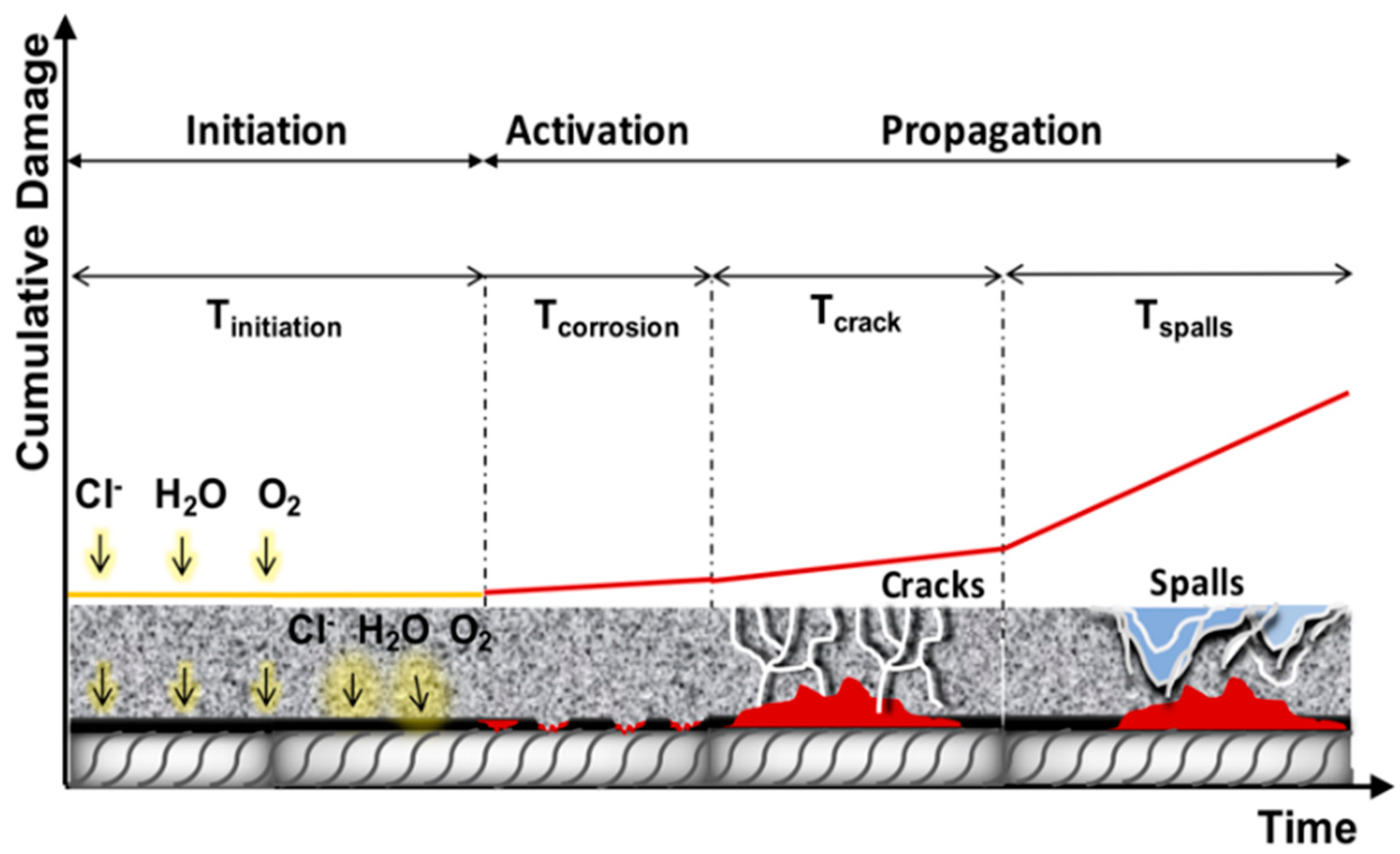
Among various models, Tuutti’s model [20] suggested the corrosion of RC structures as two main stages; initiation of corrosion and propagation of corrosion, shown in Figure 1. The stage for the initiation of corrosion starts with the diffusion of aggressive species through the concrete matrix and finishes when the depassivation and corrosion of the reinforcing steel occurs at localized sites. The initiation stage is controlled by transport processes, carbonation of concrete, and the diffusion rate of chloride ions. This initiation period can be affected by several factors such as concrete quality, concrete cover, and environmental conditions [21].

Chloride-induced corrosion is well known to be the most common and severe degradation form. Chloride ions influence the breakdown of the passive film and the initiation of localized corrosion at the reinforcing steel surface. These chloride ions can be present in the concrete matrix due to the addition of chloride-based admixtures, chloride contamination of the aggregates, and from using high chloride content water, such as seawater during the mixing process. They can also diffuse into the concrete matrix when the structure is exposed to seawater environments or deicing salts [22].

3. Probabilistic Corrosion Initiation Model: Methods

In this study, diffusion-based probabilistic models were proposed. The model selection and the parameter estimation were performed using sets of experimental data. In this section, the proposed probabilistic models, properties of experimental data sets, model selection methods, and parameter estimation methods used for this research are presented.

3.1. Diffusion-Based Probabilistic Model

To determine the time to corrosion initiation, the one dimensional Fick’s second law, which describes chloride diffusion, is commonly used [20]. In the diffusion of chloride into concrete, the chloride concentration $C$ at depth $d$ with time $t$ takes the following

$$C\left(d,t\right)=C_s\left[1-erf\left(\frac{d}{2\sqrt{Dt}}\right)\right]$$

(1)

where $C_s$ is the surface chloride concentration with units of % mass, $erf$ is the statistical error function, and $D$ is the diffusion coefficient with units of mm²/yr. The time variable $t$ is defined as the period of time from the samples exposed to the marine environment to the specific future time of interest. It is assumed that the corrosion initiates at time $t_{corr}$ when the chloride concentration at depth $d_c$ with time $t_{corr}$ reaches to the critical chloride concentration, $C_{cr}$. In the solution of this one-dimensional Fick’s second law by $\left(d_c,t_{corr}\right)=C_{cr}$, $t_{corr}$ can be first defined as below [20]

$$t_{corr}=\frac{d_c^2}{4D}{\left[er{f}^{-1}\left(1-\frac{C_{cr}}{C_s}\right)\right]}^{-2}$$

(2)

In the solution, determination of the diffusion coefficient, D, has been discussed among research papers. Many experimental research show various results of D due to the influencing parameters and the inherent uncertainties of the corrosion process. The diffusion coefficient is known to be dependent to the concrete material conditions, such as the water-to-cement (w/c) ratio, and exposure conditions including the surface chloride concentration, moisture contents in the atmosphere, dry–wet cycle of the weather, etc. [23,24]. While the most of corrosion initiation models have been developed in the deterministic format relying on the limited set of experimental data, there are a few probabilistic models suggested to predict the chloride-induced corrosion initiation time, considering the characteristics of concrete materials and exposure conditions [25,26]. In this research, we develop the probabilistic model with further improvements in the prediction of model uncertainties, contribution of each parameter and its uncertainties to the corrosion initiation, and model efficiency using the Bayesian method. Instead of maintaining all of the parameters, more focus is attained on developing the most effective model by selecting the most accurate one with the least number of parameters using the model selection criteria, which are described in the later section. Considering the nature of the function being non-negative, we could select the logarithmic variance-stabilizing transformation for homoscedastic model following Choe et al. [27] that showed the model applicability to RC bridges subject to corrosion. Therefore, the model defining $D$ can be written as:

$$\log \left[D\left(t,\mathit{\Theta }\right)\right]=\log \left[\widehat{D}\left(t,{\mathit{\theta }}_{\mathit{C}},{\mathit{\alpha }}_{\mathit{C}}\right)\right]+\sigma \epsilon$$

(3)

where $\mathit{\Theta }=\left({\mathit{\Theta }}_{\mathit{C}},{\mathit{\alpha }}_{\mathit{C}},\sigma \right)$ is the sets of unknown parameters to be estimated using Bayesian methodology, where ${\mathit{\Theta }}_{\mathit{C}}$= (${\theta }_1,{\theta }_2\dots$) represents the unknown parameters representing the diffusion coefficient for the reference case, and ${\mathit{\alpha }}_{\mathit{C}}$= (${\alpha }_1,{\alpha }_2,\dots$) is the set of parameter correction factors considering various materials and exposure conditions, which also can be estimated using Bayesian methods. For instance, in this research, ${\alpha }_1$ has been used for the correction factor for various water-to-cement ratios and ${\alpha }_2$ used for the correction factor for various concrete curing day conditions. One can develop models by expanding the model with additional correction factors ${\alpha }_3,{\alpha }_4,$ etc., for further available parameter conditions upon further data availability. $\sigma$ is the model standard deviation and $\epsilon$ is the unit random variable, which the mean is equal to 0 and the standard deviation equal to 1. The logarithm transformation results in the model uncertainties $S=exp\left(\sigma \epsilon \right)$ with the expression of the original diffusion equation as $D\left(t,\mathit{\Theta }\right)=\widehat{D}\left(t,{\mathit{\Theta }}_{\mathit{C}},{\mathit{\alpha }}_{\mathit{C}}\right)·S$.

In this study, the candidate models for the diffusion coefficient to solve the time to corrosion initiation time, $t_{corr}$, has been selected as the following:

$$\mathrm{Model}\mathrm{A}:\widehat{D}\left(t,{\mathit{\Theta }}_{\mathit{C}}\right)={\theta }_1{\left({\theta }_2/t\right)}^{{\theta }_3}$$

(4)

$$\mathrm{Model}\mathrm{B}:\widehat{D}\left(t,{\mathit{\Theta }}_{\mathit{C}},{\mathit{\alpha }}_{\mathit{C}}\right)={\alpha }_1{\theta }_1{\left({\theta }_2/t\right)}^{{\theta }_3}$$

(5)

$$\mathrm{Model}\mathrm{C}:\widehat{D}\left(t,{\mathit{\Theta }}_{\mathit{C}},{\mathit{\alpha }}_{\mathit{C}}\right)={\alpha }_1{\alpha }_2{\theta }_1{\left({\theta }_2/t\right)}^{{\theta }_3}$$

(6)

Model A assumes that the effects of the material conditions on the diffusion process are negligible, which will be used as a reference case only for this research. Model B assumes only a water-to-cement ratio has a significant effect on the diffusion, and Model C assumes that both the water-to-cement ratio and the concrete curing time have a significant effect on the diffusion process. The models result in the solution of the Fick’s law as follows:

$$\mathrm{Model}\mathrm{A}:t_{corr,A}={\left[\frac{d_c^2}{4S{\theta }_1{\left({\theta }_2\right)}^{{\theta }_3}}{\left[er{f}^{-1}\left(1-\frac{C_{cr}}{C_s}\right)\right]}^{-2}\right]}^{1/1-{\theta }_3}$$

(7)

$$\mathrm{Model}\mathrm{B}:t_{corr,B}={\left[\frac{d_c^2}{4S{\alpha }_1{\theta }_1{\left({\theta }_2\right)}^{{\theta }_3}}{\left[er{f}^{-1}\left(1-\frac{C_{cr}}{C_s}\right)\right]}^{-2}\right]}^{1/1-{\theta }_3}$$

(8)

$$\mathrm{Model}\mathrm{C}: t_{corr,C}={\left[\frac{d_c^2}{4S{\alpha }_1{\alpha }_2{\theta }_1{\left({\theta }_2\right)}^{{\theta }_3}}{\left[er{f}^{-1}\left(1-\frac{C_{cr}}{C_s}\right)\right]}^{-2}\right]}^{1/1-{\theta }_3}$$

(9)

In this research, the unknown parameters were estimated based on sets of experimental data using Bayesian updating methods. The model selection of Models A, B, and C was performed while the parameter estimation was performed by using Bayesian model selection criteria described in the later section of this paper. The time-dependent variation of the surface chloride concentration was not considered in the corrosion initiation time estimation. For the estimation, the critical chloride concentration is assumed as shown in

Table 1. Chloride threshold values (adapted from Castro-Borges et al. [7]).

Concrete Conditions	${\mathit{C}}_{\mathit{c}\mathit{r}}$ (% Concrete Mass)
		$w/c=0.46$	0.101
$w/c=0.5$	0.095
$w/c=0.53$	0.083
$w/c=0.7$	0.053
$w/c=0.76$	0.049

.

3.2. Model Parameter Estimation: Bayesian Methods

The unknown parameters $\mathit{\Theta }$ in the suggested model were estimated by the use of the observation-based updating rule [28]:

$$f\left(\mathit{\Theta }\right)=\kappa L\left(\mathit{\Theta }|\mathit{y}\right)p\left(\mathit{\Theta }\right)$$

(10)

where $p\left(\mathit{\Theta }\right)$ is the prior distribution reflecting the current knowledge about $\mathit{\Theta }$ based on our past experience, judgment, or previous models, $L\left(\mathit{\Theta }|\mathit{y}\right)$ is the likelihood function representing the objective information on $\mathit{\Theta }$ contained in a set of observations $\mathit{y}$, $\kappa ={\left[{\int }^{}L\left(\mathit{\Theta }|\mathit{y}\right)p\left(\mathit{\Theta }\right)d\mathit{\Theta }\right]}^{-1}$ is a normalizing factor, and $f\left(\mathit{\Theta }\right)$ is the posterior distribution representing our updated state of the knowledge about $\mathit{\Theta }$, which incorporates both the prior information about $\mathit{\Theta }$ included in $p\left(\mathit{\Theta }\right)$ and the new observation/data included in $L\left(\mathit{\Theta }|\mathit{y}\right)$. Once the posterior distribution of $\mathit{\Theta }$ is estimated, we could compute its mean vector, ${\mathit{M}}_{\mathit{\Theta }}$, and covariance matrix, ${{\mathbf{\sum }}^{}}_{\mathit{\Theta }\mathit{\Theta }}$.

Application of the rule in the Equation (10) can be repeated to update our modernized state of knowledge every time when new information becomes available, e.g., with any number of new data available. The updating process can be repeated any number of times. If we have m independent observations, the posterior distribution can be updated after each new sample becomes available as follows. Mathematically, the posterior distribution can be written as:

$$p\left(\mathit{\Theta }|{\mathit{y}}_1,\dots ,{\mathit{y}}_q\right)\propto p\left(\mathit{\Theta }|{\mathit{y}}_1,\dots ,{\mathit{y}}_{q-1}\right)L\left(\mathit{\Theta }|{\mathit{y}}_q\right)q=2,\dots ,m$$

(11)

where $p\left(\mathit{\Theta }|{\mathit{y}}_1\right)$ here is the prior distribution regarding the initial sample of observations, $y_1$. Repeated applications of Bayes’ theorem can then be seen as a learning process, where our present knowledge about the unknown parameters $\mathit{\Theta }$ is updated, as the new data becomes available. The likelihood function for the models in the estimation of the parameters can be written as follows based on Gardoni et al. [29]

$$L\left(\theta ,\sigma \right)\propto {\displaystyle \prod }\left\{\frac{1}{\sigma }\phi \left[\frac{DI{F}_{obsr.i}-DI{F}_{Prdc}\left({\mathit{x}}_{\mathit{i}},\mathit{\theta }\right)}{\sigma }\right]\right\}$$

(12)

3.3. Experimental Data

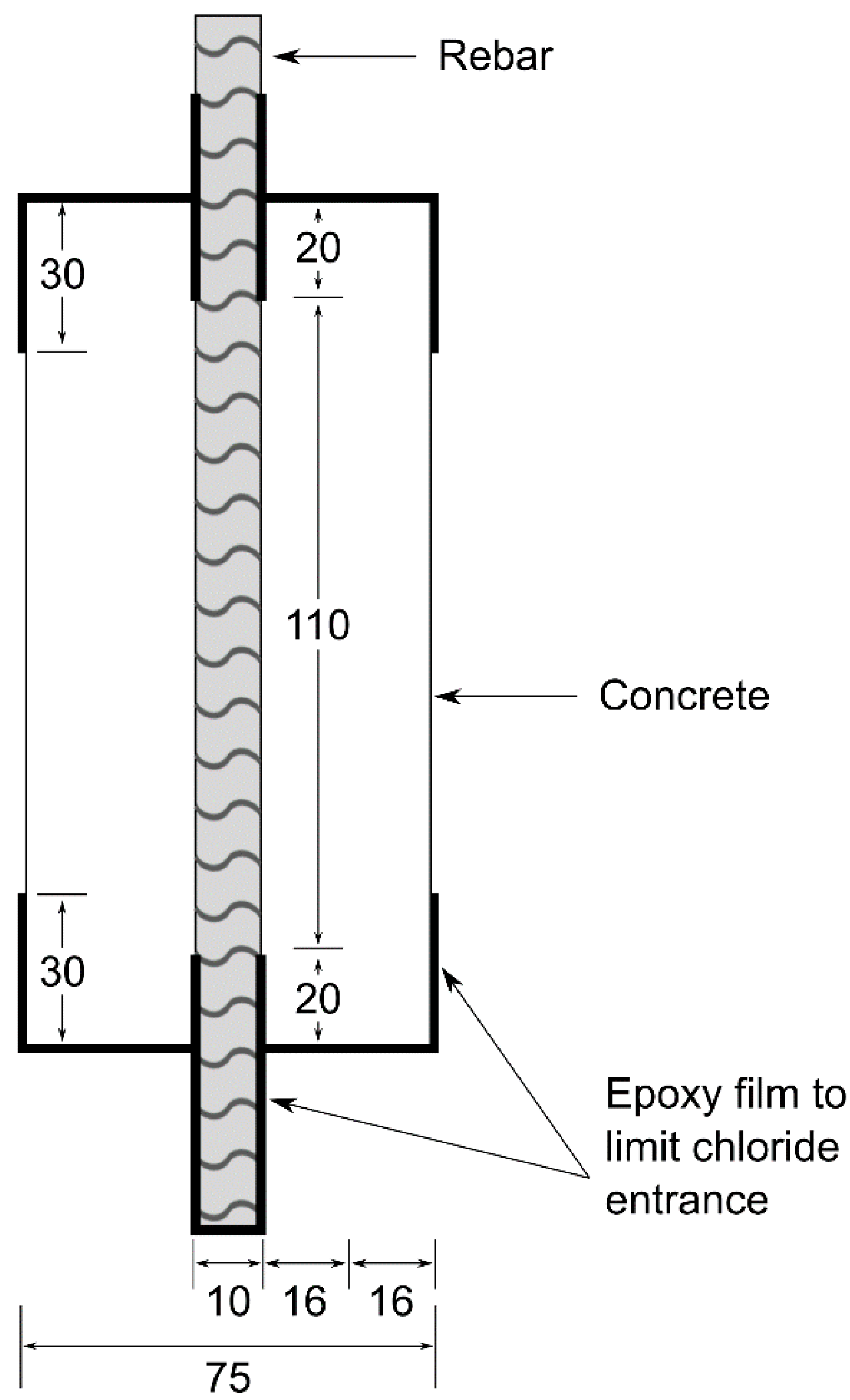
The chloride profile data points were collected over 10 years from the tropical marine environment of Yucatan Peninsula, Mexico, and previously reported in several publications [5,7,30,31]. Among the data points throughout the whole experimental period, the initial 284 data points were used for the development of corrosion initiation model. The rest of data points were considered that they were measured after the corrosion initiation, therefore not applicable to the corrosion initiation model. The samples were prepared by crushed limestone aggregates with Portland cement. Each concrete sample had a cylindrical shape with 75 mm (3 in.) in diameter and 150 mm (6 in.) in height, with a #3 (ASTM) reinforcing bar of 10 mm (0.4 in.) in diameter. Figure 2 shows a schematic description of the sample used for the experiment. The tested samples had different conditions, (1) varied water-to-cement ratios (w/c) of 0.46, 0.5, 0.53, 0.7, and 0.76 and (2) varied days of curing, 1, 3, and 7 days. The samples were exposed at the coastal region, 50 m and 100 m from the ocean. To limit the chloride entrance from top and bottom flats of the samples, the parts were sealed with epoxy coatings. The ranges of the data used for this research are provided in

Table 2. Range of the data used for this research.

Variable	Symbol	Range
Concrete Strength	$f_c^{\prime }$	14.7–34.3 MPa
Curing days	$C_d$	1–7 days
Water-to-Cement ratio	$w/c$	0.46–0.76
Distance from shore	-	50–100 m

. More experimental details including the procedure of collecting chloride concentration data for different depths and times are illustrated in previous works [5,7,30,31].

3.4. Model Selection Criteria

Once a set of alternative model options are settled, the model selection criteria need to be chosen properly. Gardoni et al. [29] suggested a step-wise deletion process for simplification of the model parameters in the application of probabilistic capacity models. Choe et al. [32] adopted two Bayesian criteria, Akaike information criteria (AICs) [33,34] and Bayesian information criteria (BICs) [35], for the application of the structural fragility increase model. In this research, Bayesian philosophy and criteria are chosen as primary model selection.

The model should be accurate, unbiased, and easily implementable in practice. In addition, as a statistical consideration, a model should be parsimonious and as simple as possible to avoid (1) loss of precision of the estimates of the overall model with its parameters due to the inclusion of unimportant terms and (2) overfitting the data.

Current model selection methods can be categorized in two classes based on their statistical performance and objectives [36]. The first class is based on the concept that no “true model” exists because the truth is very complex and cannot be modeled. Therefore, the criteria for this class are aimed to estimate the approximate true model. Akaike information criterion (AIC) is one of the most known criteria in this class. AIC was developed to select a parsimonious model for the analysis of empirical data by Akaike [33,34] The AIC provides a trade-off between the model complexity and the quality of the fit of the data. The AIC can be written as

$$AIC=-2log\left[L\left(\mathit{\Theta }\right)\right]+2N_P$$

(13)

where $N_P$ is the number of unknown parameters included in ${\mathsf{\Theta }}_k$. The second class of criteria was developed based on the concept that an exactly “true model” exists. This assumption implies that the number of parameters and the form of the true model are fixed as the number of samples, $N_S$, increases. These criteria are referred to as “constant” or “dimension-constant” criteria. Schwarz [35] provides a Bayesian argument for adopting the Bayesian information criterion (BIC), which is one of the best known “constant” criteria. The BIC penalizes the unknown parameters in terms of $N_p\log \left(N_s\right)$ that is in general a stronger penalty than the $2N_P$ used in AIC. The expression for BIC is written as

$$BIC=-2log\left[L\left(\mathit{\Theta }\right)\right]+N_{p}log\left(N_s\right)$$

(14)

BIC is known to perform well for generated data and for a large sample size of data [36]. In this paper, both AIC and BIC were used for the model selection.

In addition to these selection criteria, the mean absolute percentage error (MAPE) was computed to have a more intuitive measure of the accuracy of the candidate models [32]. The MAPE is the mean error in the model expressed as a percent of the first-order reliability method (FORM) value:

$$MAPE=\frac{1}{N_S}\left[{\displaystyle \sum }_{i=1}^{N_S}\left(\frac{\widehat{D}\left(t,{\mathit{\theta }}_{\mathit{C}},{\mathit{\alpha }}_{\mathit{C}}\right)-D_i}{D_i}\right)\right]\times 100$$

(15)

4. Probabilistic Corrosion Initiation Model: Application

The estimated results of the proposed Models A, B, and C are presented in this section. The corrosion initiation was probabilistically modeled step by step: (1) reference case, then (2) estimation of the correction factors for different material conditions. Based on the modeling, the three candidate models, Models A, B, and C are presented and evaluated. The most parsimonious model was selected based on the model selection criteria presented in the previous section.

4.1. Probabilistic Modeling: Reference Case and Additional Correction Parameters

The reference case was studied for initial parameters with a fixed consideration of material or exposure conditions. The fixed material condition was used for the case w/c = 0.46 with 7 days of curing time. This reference model was later corrected with additional sets of parameters to consider various material conditions with additional sets of data. Note that the unknown parameters, $\mathit{\Theta }$, estimated in this reference case had no meaning as a stand-alone model as the number of sample was significantly low, but only provided the best knowledge of prior sets of $\mathit{\Theta }$ for the corrected model as it is estimated with the limited information. The reference case of the diffusion coefficient can be expressed as $D\left(t,\mathit{\Theta }\right)=\widehat{D}\left(t,{\mathit{\theta }}_{\mathit{C}}\right)+\sigma \epsilon ={\theta }_1{\left({\theta }_2/t\right)}^{{\theta }_3}+\sigma \epsilon$.

Table 3. Posterior distribution of $\mathit{\Theta }$ = $\left({\theta }_1,{\theta }_{2,}{\theta }_{3,}\sigma \right)$: reference case.

$\mathit{\Theta }$	Mean	St. Dev.	Correlation Coefficient
			${\mathit{\theta }}_1$	${\mathit{\theta }}_2$	${\mathit{\theta }}_3$	$\mathit{\sigma }$
${\theta }_1$	500.0	1.000	1	-	-	-
${\theta }_2$	30.01	1.002	0.0002	1	-	-
${\theta }_3$	0.590	0.063	−0.0056	−0.0566	1	-
$\sigma$	0.263	0.053	−0.0028	−0.0526	0.0093	1

presents the results of posterior statistics for the parameters $\mathit{\Theta }=\left({\mathit{\theta }}_{\mathit{C}},\sigma \right)$. Figure 3 shows the comparison of chloride concentrations between the model predictions. The blue solid line represents the expected estimation match up of a perfect model, and the green dashed line represents the delimited region within 1 of the standard deviation. From the figure, there is a slight ambiguity of the trend that occurred from the limited number of data samples on this specific reference case. Such ambiguity becomes weaker once the model starts to include the data of other concrete conditions with extra parameters. Note that the small number of the data point in this step is further supplemented by additional data sets later in the text.

Next, based on the reference case, the model correction parameters, ${\mathit{\alpha }}_{\mathit{C}}$, were estimated, which eventually formed the Model B and C. These models considered the materials and exposure conditions with ${\mathit{\alpha }}_{\mathit{C}}=\left({\alpha }_1,{\alpha }_2\right)$, where ${\alpha }_1$ presents the correction factor of the water-to-cement ratio effect, and ${\alpha }_2$ represents the correction for the concrete curing time effect. Model B is written as $\widehat{D}\left(t,{\mathit{\theta }}_{\mathit{C}},{\mathit{\alpha }}_{\mathit{C}}\right)={\alpha }_1{\theta }_1{\left({\theta }_2/t\right)}^{{\theta }_3}$ considering the effect of the water-to-cement ratio only and Model C is as $\widehat{D}\left(t,{\mathit{\theta }}_{\mathit{C}},{\mathit{\alpha }}_{\mathit{C}}\right)={\alpha }_1{\alpha }_2{\theta }_1{\left({\theta }_2/t\right)}^{{\theta }_3}$ considering the effects both of the water-to-cement ratio and the concrete curing time.

Table 4. Posterior statistics for initial correction factors ${\alpha }_1$ and ${\alpha }_2$ for each $w/c$ and curing time.

Concrete Conditions	Distribution	${\mathit{\alpha }}_1\mathbf{Mean}$	${\mathit{\alpha }}_1$ St. Dev.	Concrete Conditions	Distribution	${\mathit{\alpha }}_2\mathbf{Mean}$	${\mathit{\alpha }}_2\mathbf{St}.\mathbf{Dev}.$
$w/c=0.46$	Normal	1.846	0.582	$Cd=1$	Normal	1.735	0.379
$w/c=0.5$	Normal	3.310	0.896
$w/c=0.53$	Normal	2.063	0.386	$Cd=3$	Normal	0.887	0.166
$w/c=0.7$	Normal	0.951	0.197
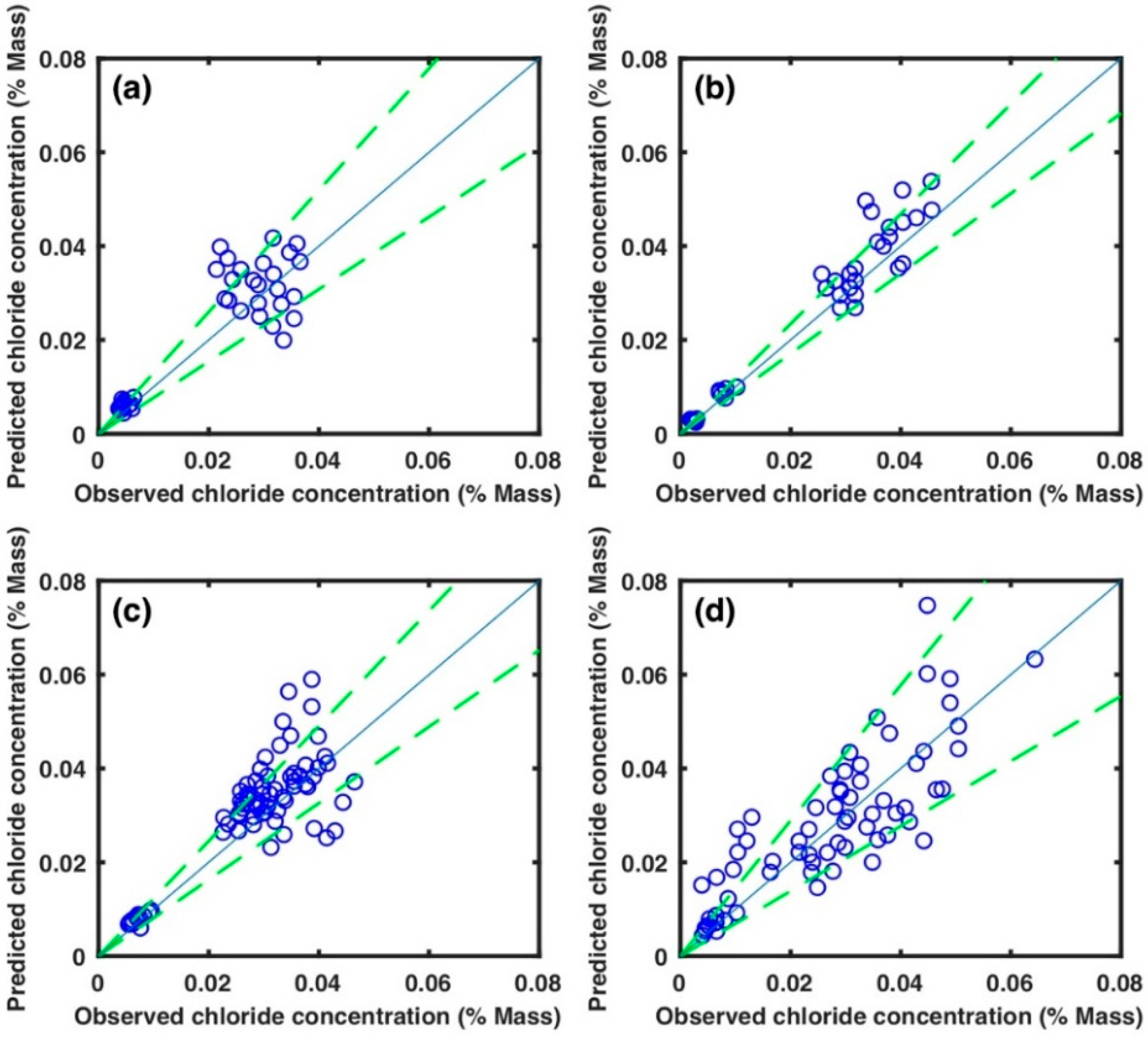
$w/c=0.76$	Normal	1.430	0.376	$Cd=7$	Normal	0.728	0.119

presents the results of the initial estimation of ${\alpha }_1$ for each w/c cases based on Model B. Compared to the reference case, the data points with shorter curing days for each w/c ratio were introduced, and they resulted in the increase of the diffusion coefficient. Although for such a trend, the results of the posterior estimation to the increased w/c ratio did not show a clear relationship. This may be caused by the uncontrolled natural weather during the experimental process. Figure 4 shows the estimation of the correction factor, ${\alpha }_1$. The figure shows a comparison between the prediction and the observation for varied concrete w/c ratio.

Table 4 also presents the results of the posterior statistics of ${\alpha }_2$ based on Model C. It is found that the longer curing contributed to the decrease of diffusion coefficient. The correction factor ${\alpha }_2$ initially studied for each curing time could be further simplified, thus ${\alpha }_2$ can be expressed as a function of $C_d$, ${\alpha }_2=-0.76\times {\left(C_d-1\right)}^{0.156}+1.735$, by a non-linear regression.

4.2. Model Selection Results: Model A, B, and C

Table 5. Model selection criteria for the candidate models.

Model	${\mathit{N}}_{\mathit{p}}$	AIC	${\mathsf{\Delta }}_{\mathit{i},\mathit{A}\mathit{I}\mathit{C}}$	BIC	${\mathsf{\Delta }}_{\mathit{i},\mathit{B}\mathit{I}\mathit{C}}$	MAPE (%)
A: $\widehat{D}\left(t,{\mathit{\Theta }}_{\mathit{C}}\right)={\theta }_1{\left({\theta }_2/t\right)}^{{\theta }_3}$	3	129.4	17.6	140.3	10.2	5.63
B: $\widehat{D}\left(t,{\mathit{\Theta }}_{\mathit{C}},{\mathit{\alpha }}_{\mathit{C}}\right)={\alpha }_1{\theta }_1{\left({\theta }_2/t\right)}^{{\theta }_3}$	4	119.9	8.1	134.5	4.4	5.61
C: $\widehat{D}\left(t,{\mathit{\Theta }}_{\mathit{C}},{\mathit{\alpha }}_{\mathit{C}}\right)={\alpha }_1{\alpha }_2{\theta }_1{\left({\theta }_2/t\right)}^{{\theta }_3}$	5	111.8	0	130.1	0	5.53

displays the results of the model selection criteria for the candidate models, including AIC, BIC, and MAPE. For both AIC and BIC, the lower value may suggest the higher efficiency of the model prediction as discussed in the previous sections in the paper. However, as a rule, the model with large variation (${\mathsf{∆}}_{AIC},{\mathsf{∆}}_{BIC}$) of AIC and BIC is to be selected instead of those with the lowest criteria. Based on the model selection criteria shown in Table 5 and the quantitative analysis of the model prediction results for each model shown in Figure 5, Model A was selected as the most parsimonious model defined in the earlier section. Although the resultant AIC and BIC were lowest at Model C, its variation from Models A and B were very minor. In addition, the qualitative observation of results in Figure 5 and the estimated MAPE shows the prediction of Model C did not significantly improve the prediction from Model A. Therefore, Model A with the least number of parameters was selected as the most parsimonious model in this research. It could also be interpreted that additional parameters for two different material conditions investigated here did not significantly impact the corrosion initiation given the range of data used for the modeling, which also contributed to deciding the model selection criterion. However, it is important to note that the parameter w/c, expressing water to cement ratio, was inexplicitly included in model A as the critical chloride concentration, $C_{cr}$, varied depending on w/c following Table 1, although it might not explicitly impact on the corrosion initiation.

Note that further availability of the experimental data may possibly change this selection if the model criteria values, AIC and BIC, had significantly changed. The selected model provided the statistically best prediction given sets of data as the Bayesian method is well known to produce unbiased model with the minimum number of samples used for the modeling.

Table 6. Posterior distribution of $\mathit{\Theta }$ =$\left({\theta }_1,{\theta }_{2,}{\theta }_{3,}\sigma \right)$: model A, selected.

$\mathit{\Theta }$	Mean	St. Dev.	Correlation Coefficient
			${\mathit{\theta }}_1$	${\mathit{\theta }}_2$	${\mathit{\theta }}_3$	$\mathit{\sigma }$
${\theta }_1$	500.0	1.000	1	-	-	-
${\theta }_2$	29.99	1.084	0.0073	1	-	-
${\theta }_3$	0.667	0.021	−0.0303	−0.4203	1	-
$\sigma$	0.301	0.013	−0.0122	−0.0522	0.0105	1

shows the posterior distribution of the selected model, Model A, as expressed in Equation (4). The updated posterior means of ${\theta }_1$, ${\theta }_2$, and ${\theta }_3$ were similar to those in the reference case. Although there was a slight increase of the posterior variance of ${\theta }_2$, but it was inferred that such an effect was compensated by the decrease of the posterior variance of ${\theta }_3$ to results in the reduction of the statistical uncertainty of the model. The model error, $\sigma$, of the updated model was higher than the one in the reference case since the model had 272 more data points to fit.

5. Corrosion Reliability and Sensitivity Measurement

5.1. Uncertainties and Model Parameters

Uncertainties that were considered in this probabilistic corrosion initiation model could be categorized into two broad types: aleatory uncertainty and epistemic uncertainty. The aleatory uncertainty is the inherent randomness, which is irreducible. The epistemic uncertainties are known to be a reducible. They include those that arise from our choice to simplify matters, lack of knowledge, measurement error, and the limited observing samples [37].

The probabilistic models suggested in this paper included the sets of random variables of $\mathit{x}=\left\{x_1,x_2,\dots \right\}$, which represent those parameters associated with the structural geometry and material conditions, and $\mathit{\Theta }=\left\{{\mathit{\Theta }}_{\mathit{C}},{\mathit{\alpha }}_{\mathit{C}}\right\}$, which represents the subsets of unknown parameters $,{\mathit{\Theta }}_{\mathit{C}}$, and correction factors, ${\mathit{\alpha }}_{\mathit{C}}$, estimated through Bayesian parameter updates using experimental data as seen in Table 3 and Table 4. The random variables $\mathit{x}$ can be the input parameters of the specific structure’s given conditions for the model users, including critical chloride concentration (normal distribution with the coefficient of variance (CoV) of 0.063), concrete cover depth (normal distribution with CoV of 0.3), and the surface chloride condition (normal distribution with CoV of 0.16).

5.2. Conditional Probability of Corrosion Initiation

The probability of failure, $P_f$, is defined as a conditional probability of corrosion initiation given surface chloride concentration and defined as a function of time t, structural and environmental properties, $\mathit{x}$. The surface chloride concentration varied in various weather conditions, distance from shore, and the material conditions. This is a parameter measurable at the site of the structures. In this research, the probability of the corrosion initiation was estimated for various ranges of surface conditions. Corrosion initiation is defined as the event where the $t_{corr}$ lays before the given time t., i.e., $t_{corr}-t\le 0$. In general consideration, the probability of corrosion initiation is suggested as follows:

$$P_f\left(t,\mathit{x},\mathit{\Theta }\right)=P\left[\underset{i}{{\displaystyle \cup }}\underset{k}{{\displaystyle \cup }}\left\{g_{ik}\left(\mathit{x},\mathit{\Theta }\right)\le 0\right\}|t,\mathit{x}\right]$$

(16)

where, $g_{ik}\left(\mathit{x},\mathit{\Theta }\right)=T_{corr}\left(\mathit{x},\mathit{\Theta }\right)-t$, k represents each failure modes, i.e., various causes of corrosion initiation, and i indicates special variability of the location, i.e., corrosion occurrences at each segment of the elements. In this research, we focused on the diffusion-induced corrosion initiation, i.e., k = 1, and no special variability has been studied. Further development can be adapted for other failure modes such as crack-induced corrosion as well as the location variability. In this research, the probability of corrosion initiation given surface chloride concentration, $C_S$, can be defined as follows:

$$P_f\left(t,\mathit{x},\mathit{\Theta }\right)=P\left[t_{corr}\left(\mathit{x},\mathit{\Theta }\right)-t\le 0|t,\mathit{x}\right]$$

(17)

For the selected Model A, the time to corrosion initiation is written as:

$$t_{corr,A}\left(\mathit{x},\mathit{\Theta }\right)={\left[\frac{d_c^2}{4{\theta }_1{\left({\theta }_2\right)}^{{\theta }_3}}{\left[er{f}^{-1}\left(1-\frac{C_{cr}}{C_s}\right)\right]}^{-2}\right]}^{1/1-{\theta }_3}$$

(18)

The results of the corrosion reliability are displayed and discussed in the following section. The corrosion reliability, $\mathsf{\beta }$, can be written in terms of the conditional probability of corrosion initiation, $P_f$, as $\mathsf{\beta }={\mathsf{\Phi }}^{-1}\left(1-P_f\right)$.

5.3. Probability of Corrosion Initiation

Examples of the conditional probability of the corrosion initiation is estimated for various given surface chloride concentration, $C_S$, which varies depending on the environmental condition where the structure sits on. The probability of the corrosion initiation is estimated as a function of the parameters given time, t, and the set of parameters $\mathit{x}$ defined earlier in the paper using the set of estimated unknown parameters of $\mathit{\Theta }$.

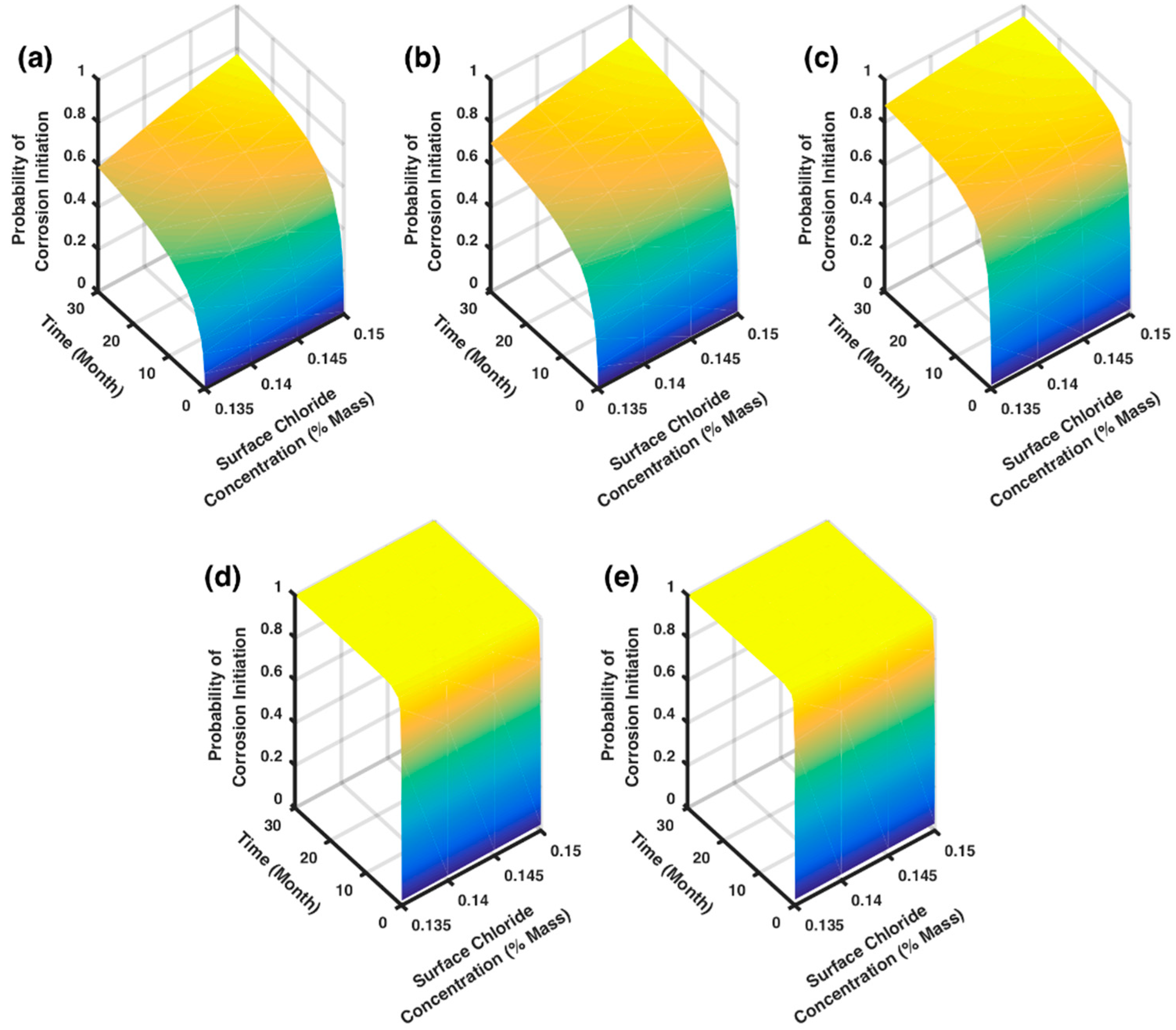
Further probability of corrosion initiation can be estimated for any structures within the range shown in Table 2 using the developed model and methods. Figure 6 shows the estimation of the conditional probability of the corrosion initiation for various w/c over time t.

It is estimated that the lower w/c ratio concrete at the same surface chloride concentration is less likely to experience corrosion initiation at the same time period. Such a trend is triggered from the critical chloride concentration for different w/c conditions, as the higher water content in the concrete may increase the susceptibility to corrosion of the rebar by increased porosity.

5.4. Parameter Sensitivity

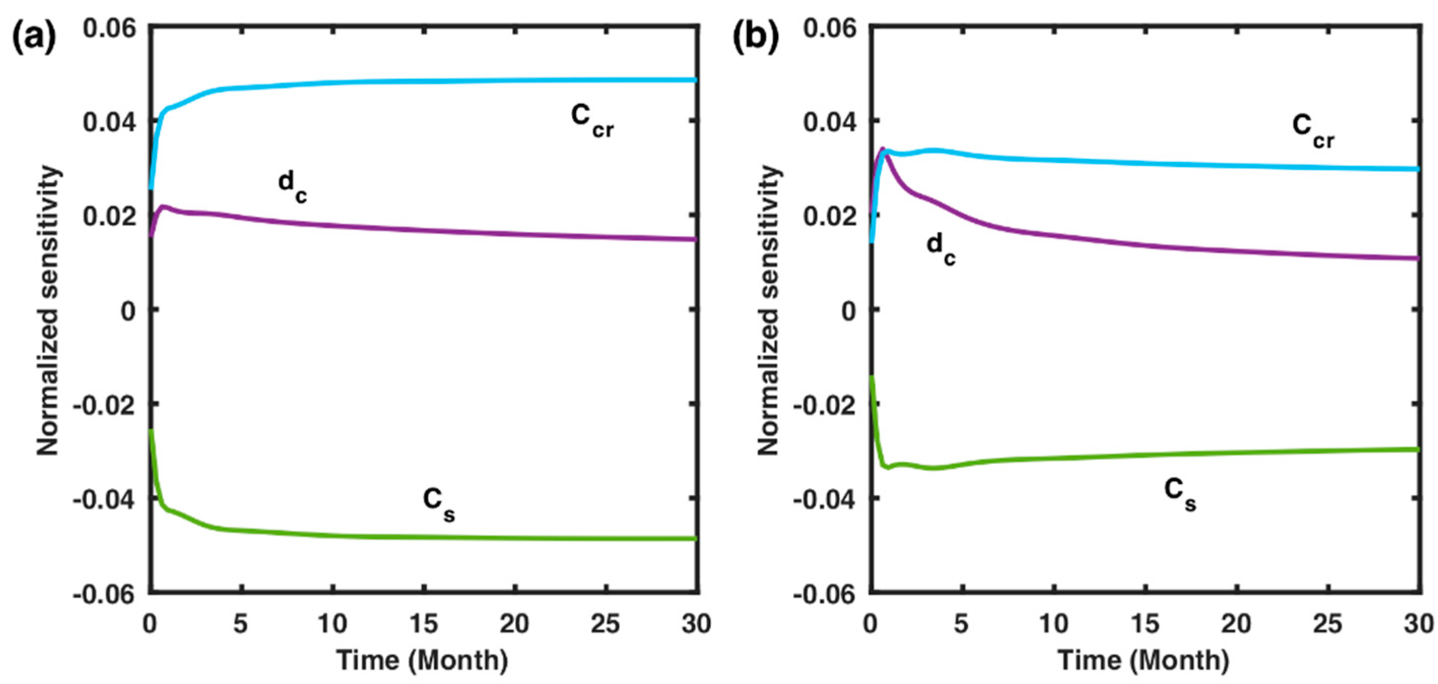
Parameter sensitivity of the reliability refers to the change of the reliability index upon the change of each parameter. The sensitivity measurement informs which parameters influences positively or negatively on the corrosion reliability and represented by $\partial \mathsf{\beta }/\partial x_i$, where $\mathsf{\beta }$ represents the reliability index and $x_i$ represents each parameter. Such results may provide physical insight and guidance in further data gathering and model development. This measure, ${\nabla }_{\left({\mathit{x}}_{\mathit{C}},{\mathit{\theta }}_{\mathit{C}}\right)}\mathsf{\beta }$ with respect to $\left({\mathit{x}}_{\mathit{C}},{\mathit{\theta }}_{\mathit{C}}\right)$ following Hohenbichler and Rackwitz [38], can be obtained by conducting a first-order reliability analysis. However, comparison among sensitivities may not be proper because the unit of each parameter varies. In this research, the normalized sensitivity of the reliability index is suggested, which is free from the parameter’s engineering unit by taking the change of the reliability upon the change of each parameter by a unit percent (%) of each parameter, which results in a form of:

$$\frac{\partial \mathsf{\beta }}{\partial x_i}\left(\frac{x_i}{100}\right)$$

(19)

The measurement methods presented above are useful as stand-alone measurements of the sensitivity and used for this research.

Figure 7 shows the results of the normalized sensitivity analysis of the corrosion initiation model reliability with respect to each associated parameter. Under the specified conditions, it is observed that the parameters $C_{cr}$ and $d_c$ are positively affecting the reliability of corrosion initiation. It is interpreted that the unit percent increase of those parameters results in the increase of the reliability accordingly. The other parameter in the figure, $C_s$, shows the negative values of normalized sensitivity, and it represents the unit increase of such parameter results in the decrease of the estimated reliability. The results infer the way to improve the reliability of the corrosion initiation estimation by controlling the parameters. For example, the $C_{cr}$ can be one possible parameter to improve the reliability of the corrosion initiation estimation by controlling the pH level of the concrete matrix, which might be less complicated compared to controlling $C_s,$ which is normally coming from the natural environment. The results agree with existing literatures [39]. Although there were no previous probabilistic models that include the sensitivity analysis to the reliability, it has reported that $C_{cr}$ and $C_s$ are the most sensitive parameters in the general term.

5.5. Importance of the Variability

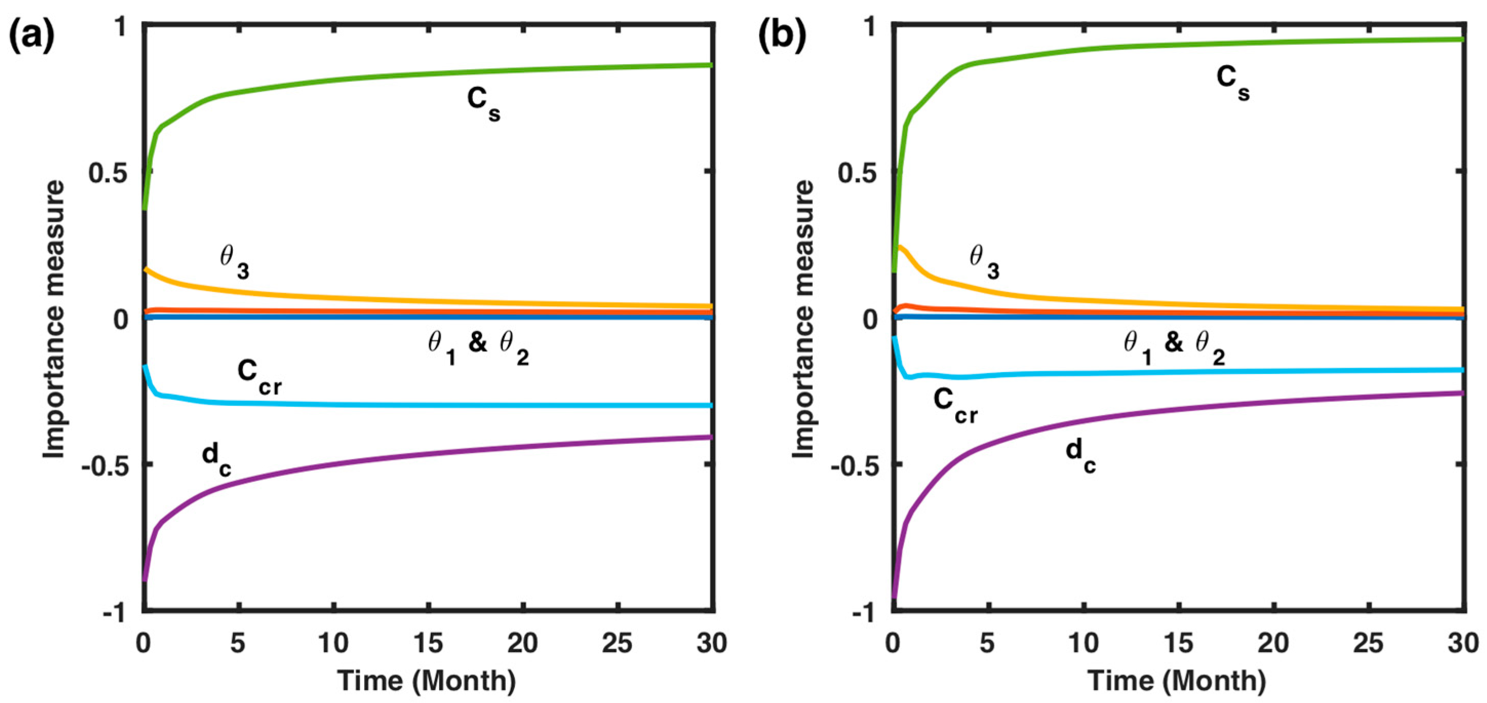
The importance measure informs, which parameter’s randomness is influencing the most on the corrosion reliability. Some random variables have larger effects on the variance of the limit state function and thus are more important and vice versa. Following Der Kiureghian and Ke [40], we obtained a measure of importance $\gamma$ as:

$${\gamma }^T=\frac{{\mathit{\alpha }}^T{\mathit{J}}_{{\mathit{u}}^{\mathit{\ast }},{\mathit{z}}^{\mathit{\ast }}}\mathit{S}{\mathit{D}}^{\mathit{\prime }}}{\Vert {\mathit{\alpha }}^T{\mathit{J}}_{{\mathit{u}}^{\mathit{\ast }},{\mathit{z}}^{\mathit{\ast }}}\mathit{S}{\mathit{D}}^{\mathit{\prime }}\Vert }$$

(20)

where $\mathit{z}$ is the vector of the random variables, $\mathit{z}=\left(\mathit{X}\mathit{C},{\mathit{\theta }}_{\mathit{C}}\right)$ and ${\mathit{J}}_{{\mathit{u}}^{\mathit{\ast }},{\mathit{z}}^{\mathit{\ast }}}$ is the Jacobian of the probability transformation from the original space $\mathit{z}$ to the standard normal space $\mathit{u}$, to the coordinates of the design point ${\mathit{z}}^{\mathit{\ast }}$. Matrix $\mathit{S}{\mathit{D}}^{\mathit{\prime }}$ is the standard deviation matrix of equivalent normal variables ${\mathit{z}}^{\mathit{\prime }}$ defined by the linearized inverse transformation ${\mathit{z}}^{\mathit{\prime }}={\mathit{z}}^{\mathit{\ast }}+{\mathit{J}}_{{\mathit{z}}^{\mathit{\ast }},{\mathit{u}}^{\mathit{\ast }}}$ at the design point.

Figure 8 shows the importance measures for the parameters in the reliability model for corrosion initiation. It is noted that the importance measure shows the opposite sign to the sensitivity measures. Thus, it is interpreted that the higher randomness of the positively affecting parameter decreased the reliability and vice versa. The rank of the importance shows the similar trend compared to the sensitivity with the opposite sign. Figure 8 also suggests that $C_s$, $C_{cr}$, and $d_c$ are the most important sources of uncertainty throughout the time period. Meanwhile, ${\theta }_1$, ${\theta }_2$, and ${\theta }_3$ were estimated to have the smallest effect on the variance of the model as their importance reduced close to zero. This implies that the parameters with the least importance may be considered as constant to further simplify the model.

6. Conclusions

The paper proposed a framework to develop probabilistic models that predict the corrosion initiation time and its inherent uncertainties of the RC structures. The model developed through the framework can account for as many acting factors as possible to begin with, e.g., material properties and exposure conditions. However, the Bayesian model selection process resulted in the most parsimonious models, i.e., the model with simplest expression and the least number of parameters to avoid the loss of prediction accuracy. The framework included the probabilistic modeling with the Bayesian parameter updating, Bayesian model selection to improve the model efficiency, the reliability analyses to predict the corrosion initiation or to test the developed model, and the sensitivity analyses to inform the decision making to improve the corrosion reliability.

• Model selection criteria of ${\mathsf{\Delta }}_{i,AIC}$ and ${\mathsf{\Delta }}_{i,BIC}$ were used and selected Model A as the statistically most efficient model among the developed models reflecting the prediction results. Model A dropped w/c as an explicit parameter. However, w/c is inexplicitly considered in Model A as a parameter to determine the critical threshold of the chloride concentration. The model variability and parameter uncertainties were estimated for the given set of experimental data. The Bayesian updating method used for the research allows further updating of the model upon the availability of future data.
• Based on the developed model, the corrosion reliability was estimated in terms of the conditional probability of the corrosion initiation under given surface chloride concentration for example structures. The developed model predicts the probability of the corrosion initiation of any other RC structures within the range shown in Table 2, which is the range of the parameters of data sets used for this model. Further, the framework and methods presented in the paper can be generally used for outside of the range upon any future availability of new sets of data.
• The sensitivity analyses showed that the critical threshold of chloride concentration, $C_{cr}$, the surface chloride concentration, $C_s$, and the cover depth of the concrete structures, $d_c$, are the most effective parameters to increase the reliability of corrosion initiation. The importance measure showed that controlling of the uncertainties of the surface chloride concentration, $C_s$, is the most efficient to increase the corrosion reliability out of the entire set of parameters.

References

- Koch, G.H.; Brongers, M.P.; Thompson, N.G.; Virmani, Y.P.; Payer, J.H. Corrosion Cost and Preventive Strategies in the United States; Federal Highway Administration: Washington, DC, USA, 2002.
- Irie, H.; Yoshida, Y.; Sakurada, Y.; Ito, T. Non-destructive-testing methods for concrete structures. NTT Tech. Rev. 2008, 6, 1–8. [Google Scholar]
- Thanapol, Y.; Akiyama, M.; Frangopol, D.M. Updating the Seismic Reliability of Existing RC Structures in a Marine Environment by Incorporating the Spatial Steel Corrosion Distribution: Application to Bridge Piers. J. Bridge Eng. 2016, 21, 04016031. [Google Scholar] [CrossRef]
- Kim, J.; Gucunski, N.; Dinh, K. Similarities and differences in bare concrete deck deterioration curves from multi NDE technology surveys. In Proceedings of the Health Monitoring of Structural and Biological Systems 2016; International Society for Optics and Photonics, Las Vegas, NV, USA, 21–24 March 2016; Volume 9805, p. 98052H. [Google Scholar]
- Castro, P.; De Rincon, O.; Pazini, E. Interpretation of chloride profiles from concrete exposed to tropical marine environments. Cem. Concr. Res. 2001, 31, 529–537. [Google Scholar] [CrossRef]
- Sandberg, P.; Tang, L.; Andersen, A. Recurrent studies of chloride ingress in uncracked marine concrete at various exposure times and elevations. Cem. Concr. Res. 1998, 28, 1489–1503. [Google Scholar] [CrossRef] [Green Version]
- Castro-Borges, P.; Balancán-Zapata, M.; López-González, A. Analysis of Tools to Evaluate Chloride Threshold for Corrosion Onset of Reinforced Concrete in Tropical Marine Environment of Yucatán, México. J. Chem. 2013, 2013, 1–8. [Google Scholar] [CrossRef]
- Oh, B.H.; Jang, S.Y.; Shin, Y.S. Experimental investigation of the threshold chloride concentration for corrosion initiation in reinforced concrete structures. Mag. Concr. Res. 2003, 55, 117–124. [Google Scholar] [CrossRef]
- Ann, K.Y.; Ahn, J.H.; Ryou, J.S. The importance of chloride content at the concrete surface in assessing the time to corrosion of steel in concrete structures. Constr. Build. Mater. 2009, 23, 239–245. [Google Scholar] [CrossRef]
- Val, D.V.; Trapper, P.A. Probabilistic evaluation of initiation time of chloride-induced corrosion. Reliab. Eng. Syst. Saf. 2008, 93, 364–372. [Google Scholar] [CrossRef]
- Bastidas-Arteaga, E.; Chateauneuf, A.; Sánchez-Silva, M.; Bressolette, P.; Schoefs, F. A comprehensive probabilistic model of chloride ingress in unsaturated concrete. Eng. Struct. 2011, 33, 720–730. [Google Scholar] [CrossRef] [Green Version]
- Arora, P.; Popov, B.N.; Haran, B.; Ramasubramanian, M.; Popova, S.; White, R.E. Corrosion initiation time of steel reinforcement in a chloride environment—A one dimensional solution. Corros. Sci. 1997, 39, 739–759. [Google Scholar] [CrossRef]
- Engelund, S.; Sørensen, J.D. A probabilistic model for chloride-ingress and initiation of corrosion in reinforced concrete structures. Struct. Saf. 1998, 20, 69–89. [Google Scholar] [CrossRef]
- Castaneda, H.; Karsilaya, A.; Okeil, A.; Taha, M.R. A Comprehensive Reliability-Based Framework for Corrosion Damage Monitoring and Repair Design of Reinforced Concrete Structures. TranSet Data 2018, 26, 65. [Google Scholar]
- Bertolini, L.; Elsener, B.; Pedeferri, P.; Redaelli, E.; Polder, R.B. Corrosion of Steel in Concrete: Prevention, Diagnosis, Repair; John Wiley & Sons: Hoboken, NJ, USA, 2013; ISBN 978-3-527-65171-9. [Google Scholar]
- Freire, L.; Nóvoa, X.R.; Montemor, M.F.; Carmezim, M.J. Study of passive films formed on mild steel in alkaline media by the application of anodic potentials. Mater. Chem. Phys. 2009, 114, 962–972. [Google Scholar] [CrossRef]
- Nagayama, M.-I.; Cohen, M. The Anodic Oxidation of Iron in a Neutral Solution I. The Nature and Composition of the Passive Film. J. Electrochem. Soc. 1962, 109, 781–795. [Google Scholar] [CrossRef]
- Sánchez, M.; Takenouti, H.; García-Jareño, J.J.; Vicente, F.; Alonso, C. A theoretical approach of impedance spectroscopy during the passivation of steel in alkaline media. Electrochim. Acta 2009, 54, 7222–7226. [Google Scholar] [CrossRef]
- El Haleem, S.A.; El Aal, E.E.A.; El Wanees, S.A.; Diab, A. Environmental factors affecting the corrosion behaviour of reinforcing steel: I. The early stage of passive film formation in Ca(OH)2 solutions. Corros. Sci. 2010, 52, 3875–3882. [Google Scholar] [CrossRef]
- Tuutti, K. Corrosion of Steel in Concrete. Ph.D. Thesis, Lund University, Swedish Cement and Concrete Research Institute, Stockholm, Sweden, 1982. [Google Scholar]
- Böhni, H. Corrosion in Reinforced Concrete Structures; Woodland Publishing: Chelmsford, UK, 2005; ISBN 978-1-84569-043-4. [Google Scholar]
- Broomfield, J.P. Corrosion of Steel in Concrete: Understanding, Investigation and Repair; CRC Press: Boca Raton, FL, USA, 2003. [Google Scholar]
- Luping, T. Chloride Transport in Concrete—Measurement and Prediction. Ph.D. Thesis, Chalmers University of Technology, Gothenburg, Sweden, 1996. [Google Scholar]
- Mangat, P.S.; Molloy, B.T. Prediction of long term chloride concentration in concrete. Mater. Struct. 1994, 27, 338–346. [Google Scholar] [CrossRef]
- Choe, D.-E.; Gardoni, P.; Rosowsky, D.; Haukaas, T. Probabilistic capacity models and seismic fragility estimates for RC columns subject to corrosion. Reliab. Eng. Syst. Saf. 2008, 93, 383–393. [Google Scholar] [CrossRef]
- DuraCrete. Statistical Quantification of the Variables in the Limit State Functions; The European Union-Brite EuRam III-Contract BRPR-CT95-0132-Project BE95-1347/R9; European Union: Brussels, Belgium, 2000. [Google Scholar]
- Choe, D.-E.; Gardoni, P.; Rosowsky, D.; Haukaas, T. Seismic fragility estimates for reinforced concrete bridges subject to corrosion. Struct. Saf. 2009, 31, 275–283. [Google Scholar] [CrossRef]
- Box, G.E.P.; Tiao, G.C. Bayesian Inference in Statistical Analysis; John Wiley & Sons: Hoboken, NJ, USA, 2011; ISBN 978-1-118-03144-5. [Google Scholar]
- Gardoni, P.; Der Kiureghian, A.; Mosalam, K.M. Probabilistic Capacity Models and Fragility Estimates for Reinforced Concrete Columns based on Experimental Observations. J. Eng. Mech. 2002, 128, 1024–1038. [Google Scholar] [CrossRef]
- Castro, P.; Veleva, L.; Balancán, M. Corrosion of reinforced concrete in a tropical marine environment and in accelerated tests. Constr. Build. Mater. 1997, 11, 75–81. [Google Scholar] [CrossRef]
- Castro, P.; Sanjuán, M.A.; Genesca, J. Carbonation of concretes in the Mexican Gulf. Build. Environ. 2000, 35, 145–149. [Google Scholar] [CrossRef]
- Choe, D.-E.; Gardoni, P.; Rosowsky, D. Fragility Increment Functions for Deteriorating Reinforced Concrete Bridge Columns. J. Eng. Mech. 2010, 136, 969–978. [Google Scholar] [CrossRef]
- Akaike, H. A Bayesian analysis of the minimum AIC procedure. Ann. Inst. Stat. Math. 1978, 30, 9–14. [Google Scholar] [CrossRef]
- Akaike, H. A new look at the Bayes procedure. Biometrika 1978, 65, 53–59. [Google Scholar] [CrossRef]
- Schwarz, G. Estimating the Dimension of a Model. Ann. Stat. 1978, 6, 461–464. [Google Scholar] [CrossRef]
- Burnham, K.P.; Anderson, D.R. Model Selection and Multimodel Inference: A Practical Information-Theoretic Approach; Springer Science & Business Media: Berlin/Heidelberg, Germany, 2003; ISBN 978-0-387-95364-9. [Google Scholar]
- Der Kiureghian, A. Measures of Structural Safety Under Imperfect States of Knowledge. J. Struct. Eng. 1989, 115, 1119–1140. [Google Scholar] [CrossRef]
- Hohenbichler, M.; Rackwitz, R. First-order concepts in system reliability. Struct. Saf. 1982, 1, 177–188. [Google Scholar] [CrossRef]
- Zhang, J.; Lounis, Z. Sensitivity analysis of simplified diffusion-based corrosion initiation model of concrete structures exposed to chlorides. Cem. Concr. Res. 2006, 36, 1312–1323. [Google Scholar] [CrossRef] [Green Version]
- Der Kiureghian, A.; Ke, J.B. Finite-element based reliability analysis of frame structures. In Proceedings of the Proc. 4th Int. Conference on Structural Safety and Reliability, Kobe, Japan, 27–29 May 1985; pp. 395–404. [Google Scholar]
Figure 1.
Initiation and propagation of the corrosion of reinforcing steel in concrete (adapted from Tuutti [20]).
Figure 2.
Schematic description of the specimen used in mm scale (adapted from Castro-Borges et al. [7]).
Figure 3.
Reference case: (a) model prediction vs. observation and (b) prediction error.
Figure 4.
Example parameter estimation of correction factor : (a) w/c = 0.46, (b) w/c = 0.5, (c) w/c = 0.53, and (d) w/c = 0.7.
Figure 5.
Model prediction vs. observation and prediction error; Model A: (a,b), Model B: (c,d), and Model C: (e,f).
Figure 6.
Estimated probability of corrosion initiation: (a) w/c = 0.46, (b) w/c = 0.5, (c) w/c = 0.53, (d) w/c = 0.7, and (e) w/c = 0.76.
Figure 7.
Example normalized sensitivity measures: (a) w/c = 0.5 and = 0.14 and (b) w/c = 0.76 and = 0.14.
Figure 8.
Example importance measures: (a) w/c = 0.5 and = 0.14 and (b) w/c = 0.76 and = 0.14.