Indirect Galvanostatic Pulse in Wenner Configuration: Numerical Insights into Its Physical Aspect and Its Ability to Locate Highly Corroding Areas in Macrocell Corrosion of Steel in Concrete

 , and
, and
Abstract
:1. Introduction
2. Materials and Methods
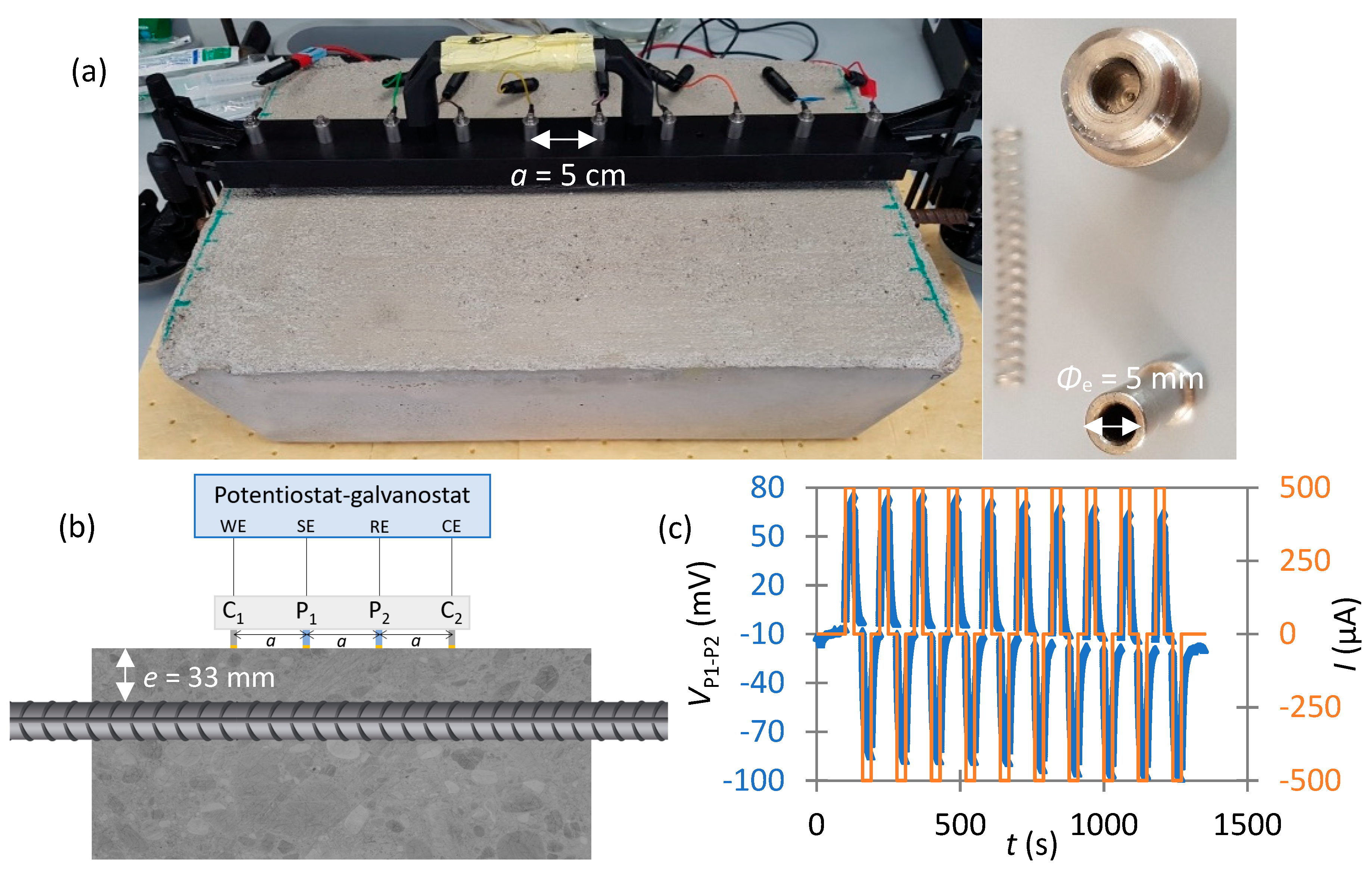
2.1. Experiments
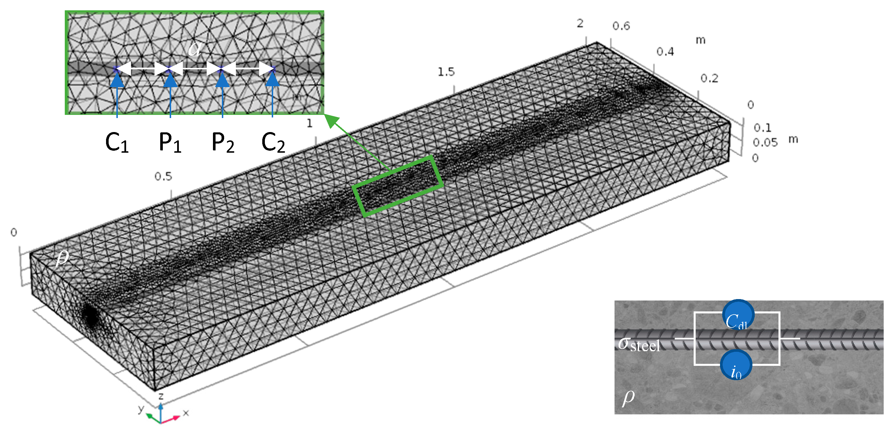
2.2. Simulations
3. Experimental Results
4. Numerical Results
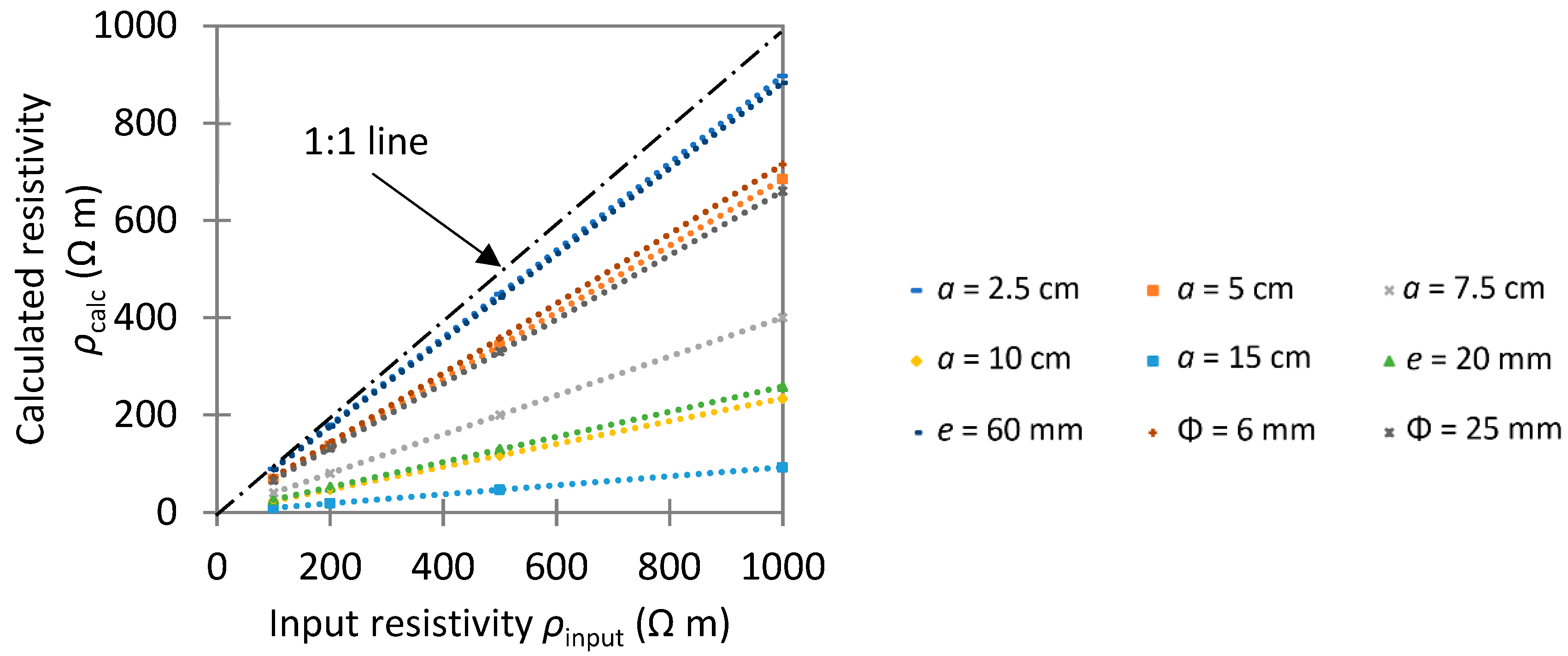
4.1. Unreinforced Specimen: Geometric Factor
4.2. Uniform Corrosion: Parametric Study
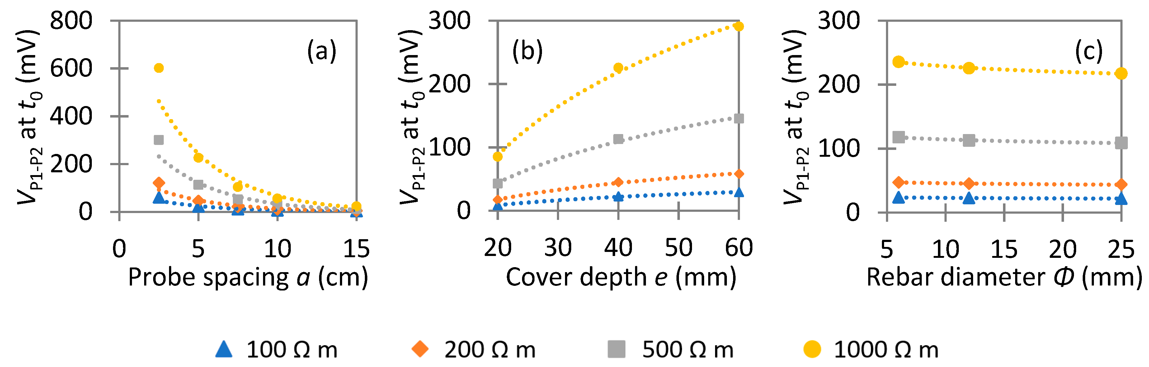
4.2.1. Instantaneous Ohmic Drop
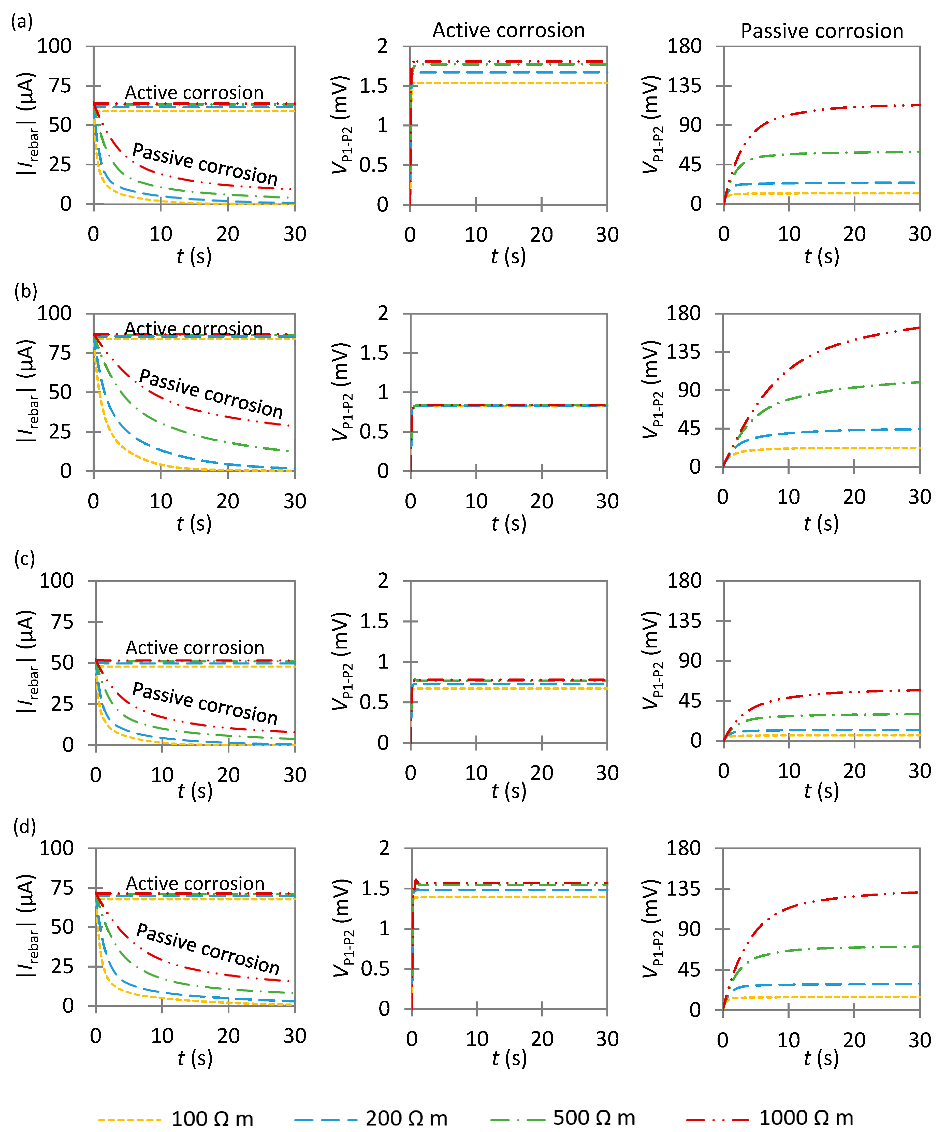
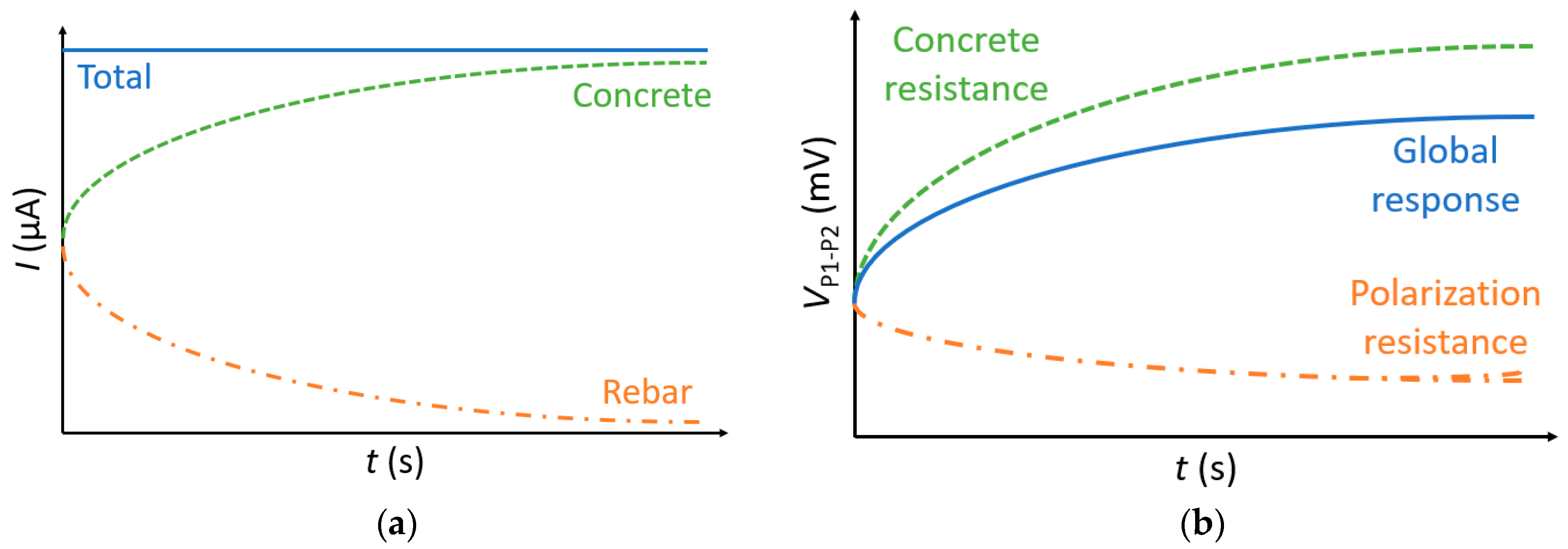
4.2.2. Transient Potential
4.3. Non-Uniform Corrosion: Detection of the Actively Corroding Area
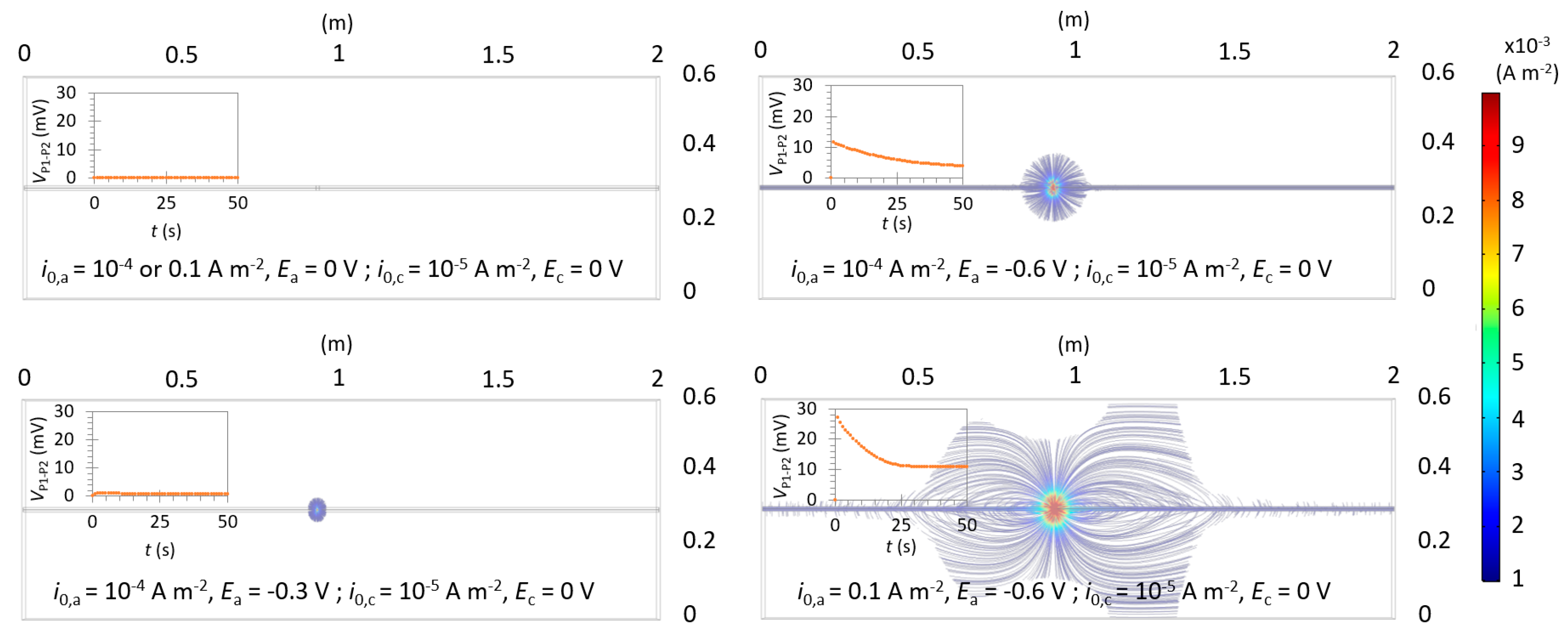
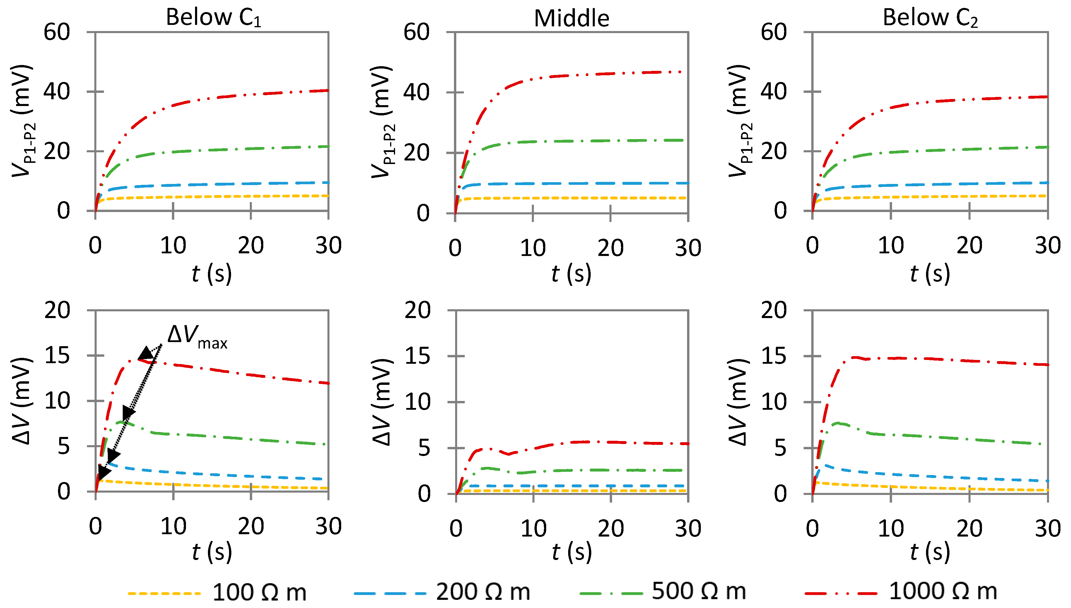
4.3.1. Influence of an Anode with a Low Anodic Exchange Current Density
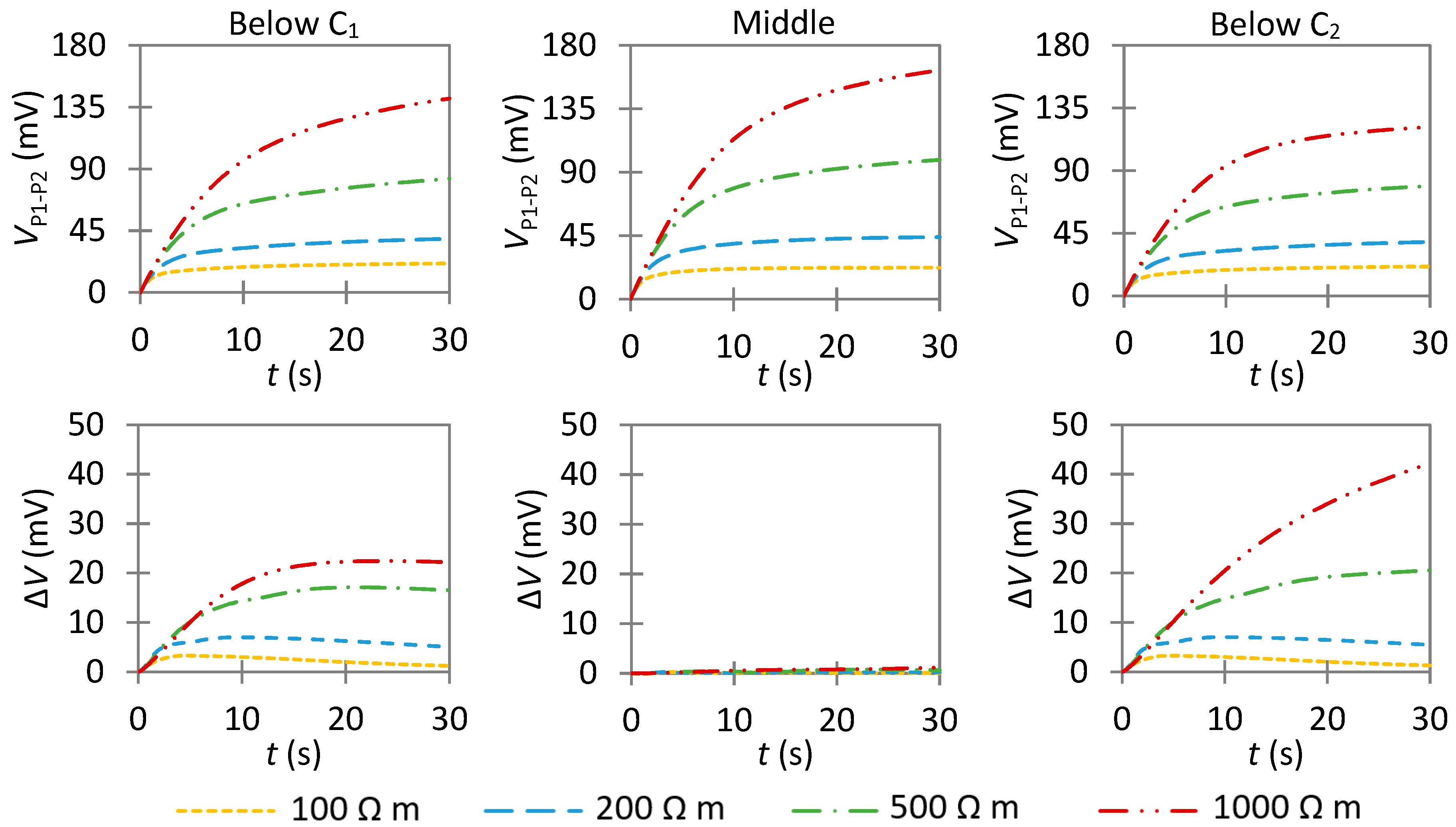
4.3.2. Influence of an Anode with a High Anodic Exchange Current Density
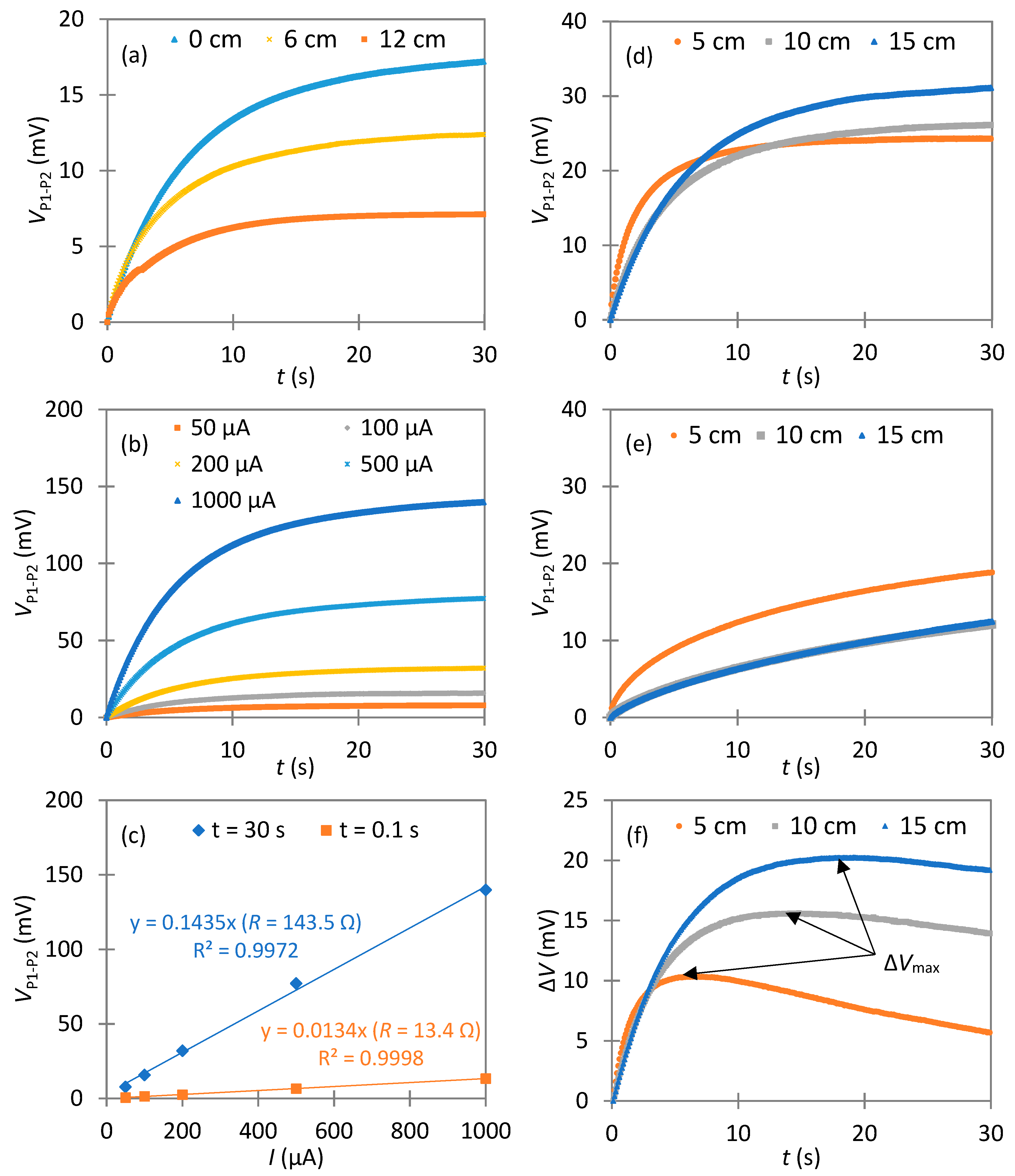
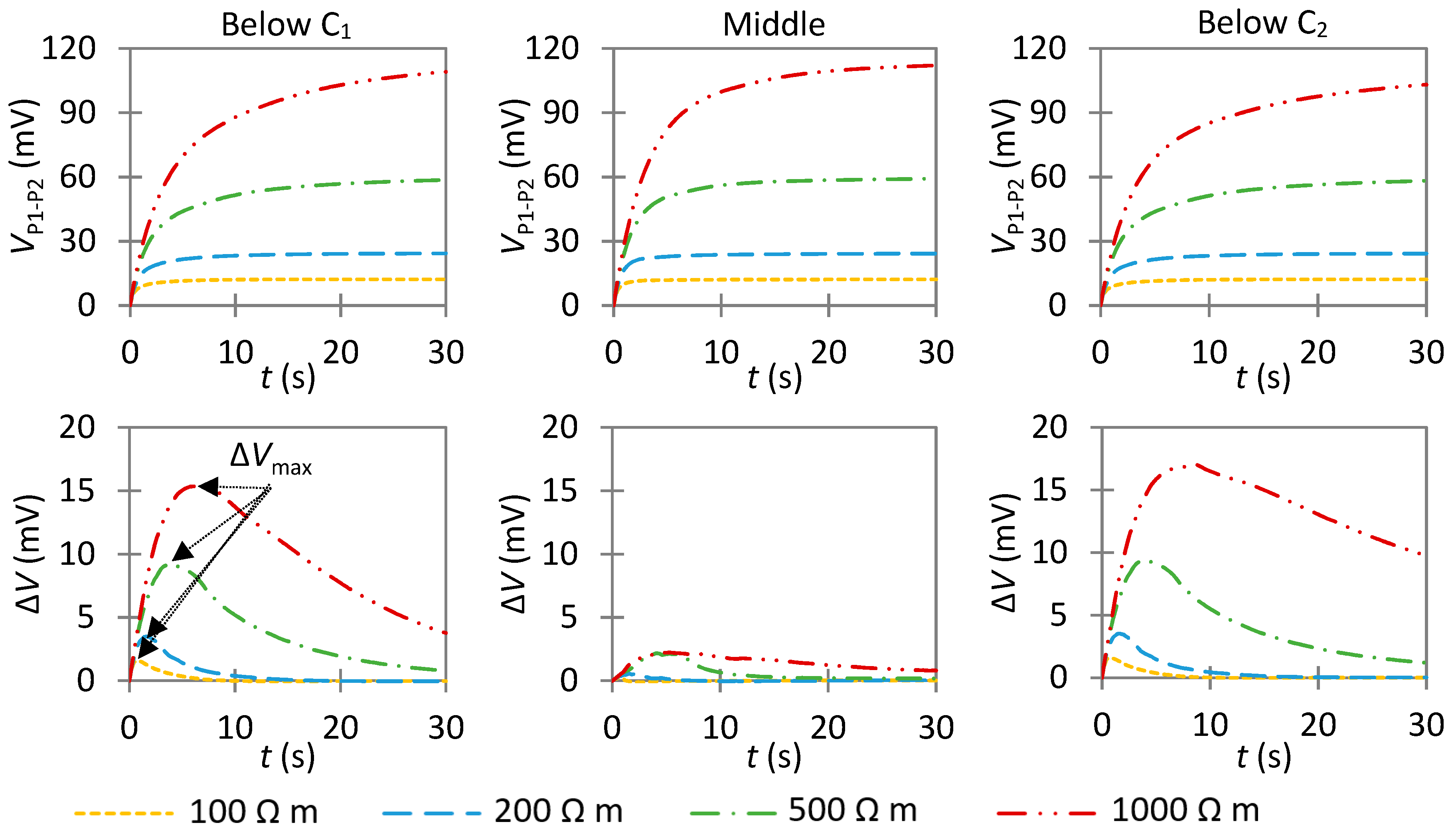
4.3.3. Influence of the Probe Spacing
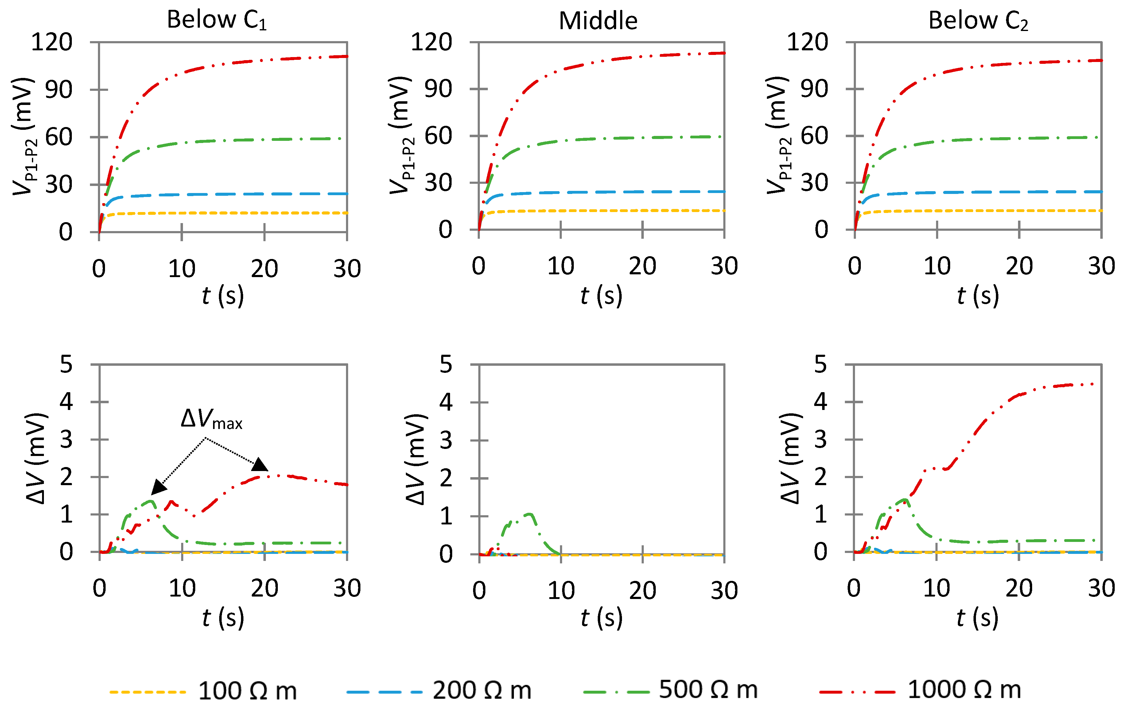
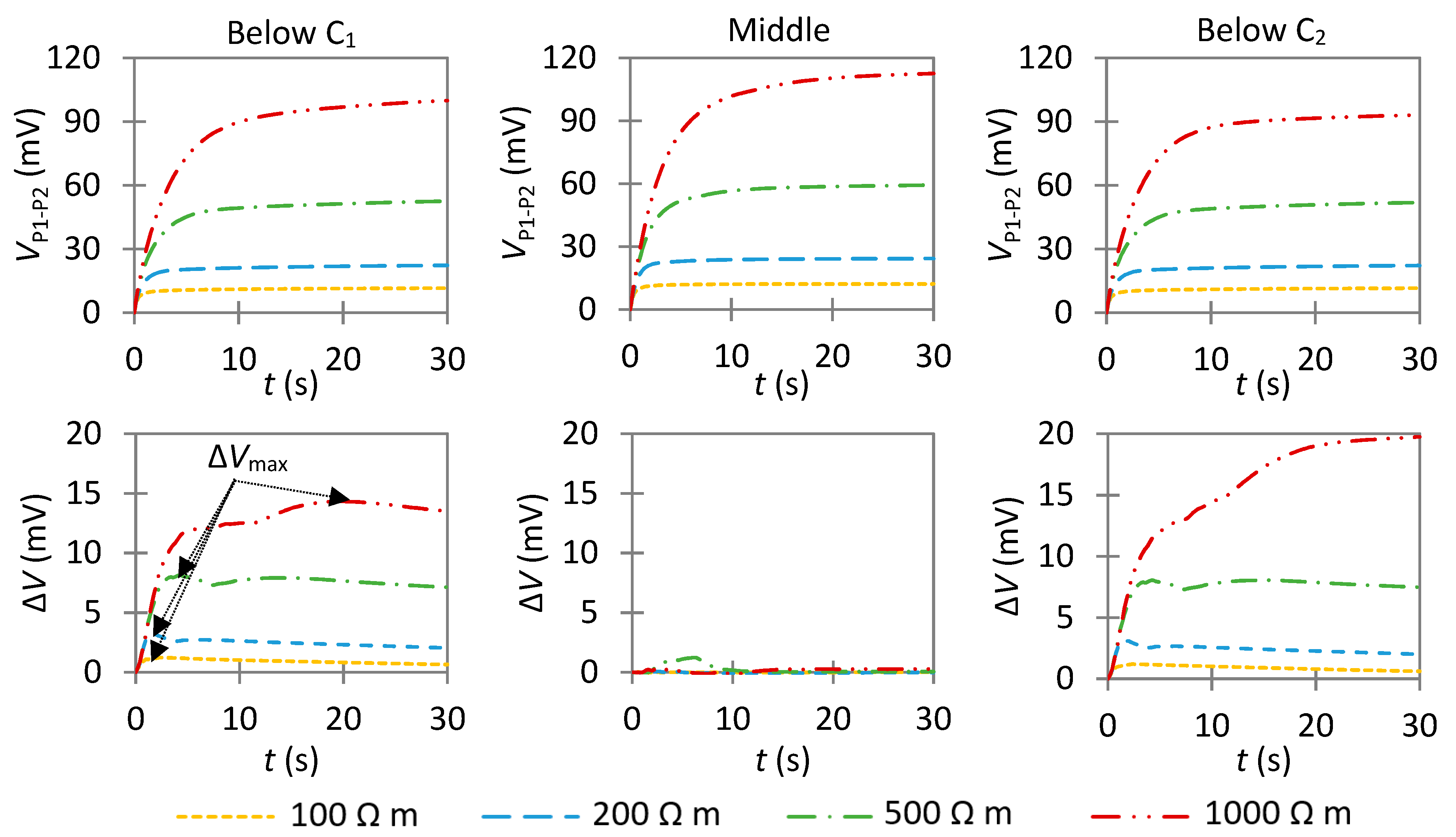
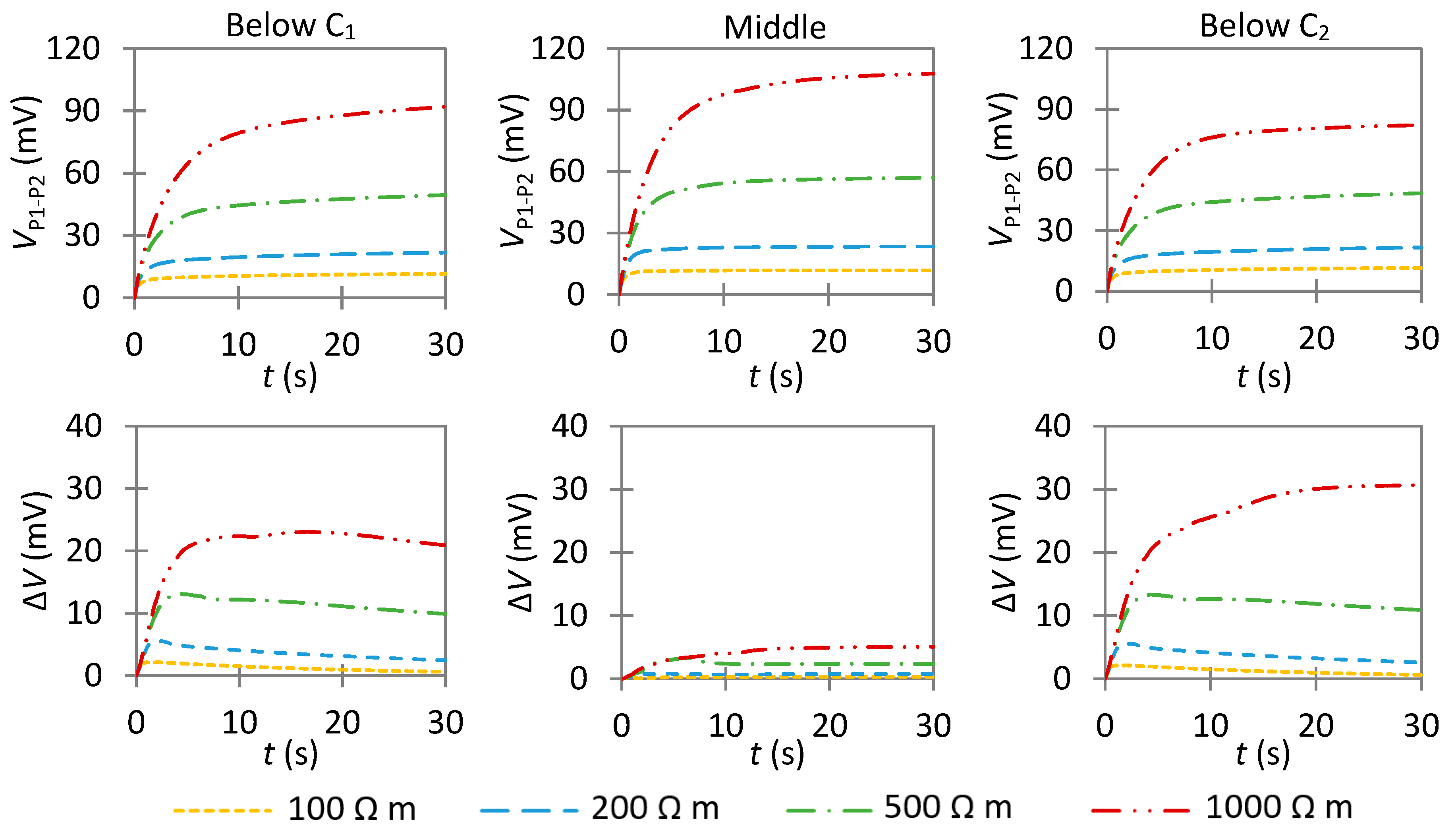
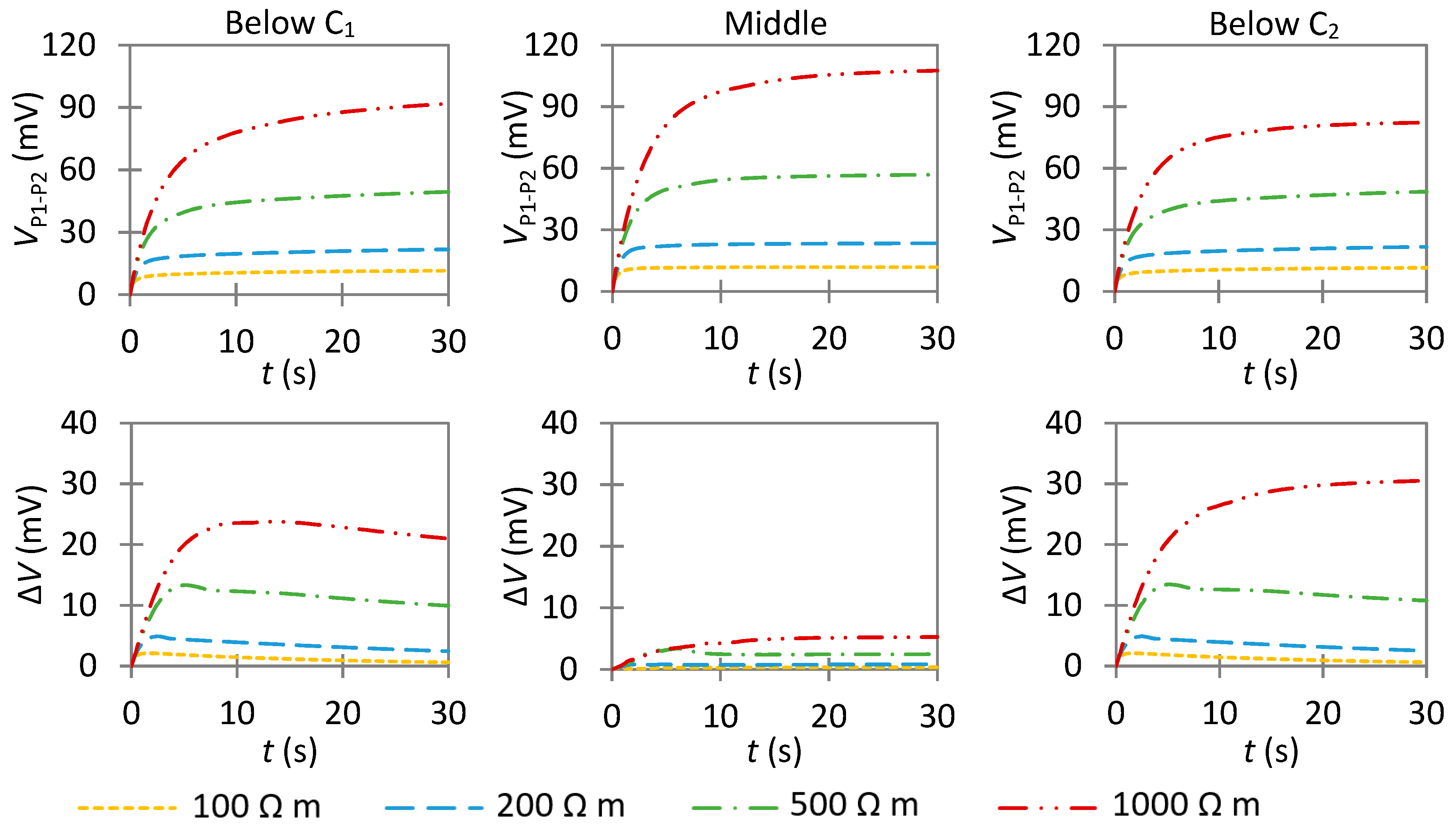
4.3.4. Influence of the Double-Layer Capacitance of the Anode
5. Discussion
5.1. Rebar Effect on the Instantaneous Ohmic Drop
5.2. Ability of Indirect GP to Detect Localized Corrosion in Wenner Configuration
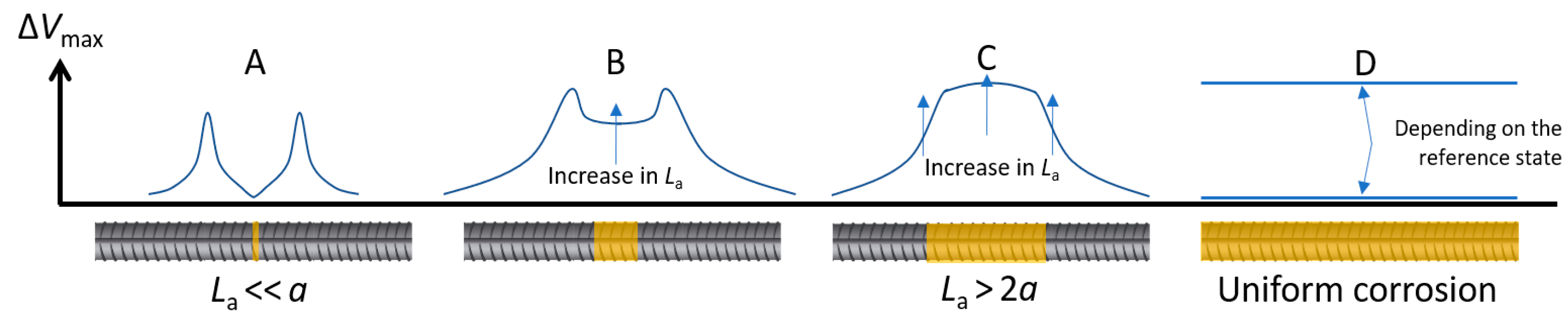
- Case A: If ΔVmax is close to 0 in the middle of two well-defined—but not necessarily symmetric—peaks, it is the result of a much smaller anode than the probe spacing (La << a);
- Case B: As La increases, the value of ΔVmax in the middle of the two peaks also increases. As indicated by further simulations (Figure S10), it becomes similar to the value of the peaks when La ≃ 1.5–2a for e = 40 mm;
- Case C: If ΔVmax is high over a large section with a maximum value close to its center, it is the result of an anode larger than the probe spacing (La > 2a). This indicates a large actively corroding section of the rebar; and
- Case D: If ΔVmax remains around 0, it is the result of uniform corrosion along the investigated area. It can either represent a fully passive rebar, a passive rebar with an anode with a low exchange current density, or an actively corroding rebar if the considered reference state also corresponds to active corrosion. If ΔVmax is similar along the rebar and different than 0, this indicates an actively corroding rebar with a passive reference state.
5.3. Comparison of Indirect GP with Indirect EIS
5.4. Towards a Quantification of the Corrosion Rate in Non-Uniform Corrosion?
5.5. Implication for Practical Applications on RC Structures
5.6. Necessity of Electrical/Electrochemical Tomography
6. Conclusions
- (1)
- Sample geometry is an important parameter when performing any experiments or numerical simulations. An accurate geometric factor must be determined case-by-case, depending on specimen size and probe spacing, to convert concrete resistance into concrete resistivity.
- (2)
- The instantaneous ohmic drop is largely affected by the presence of rebar that acts initially as a short-circuit. This rebar effect decreases the value of concrete resistivity, especially when the measurement is done right above the rebar. It mainly depends on the probe spacing, the cover depth, and the geometry of the slab. It was also shown that the electrochemical state of the rebar has no influence on the rebar effect; thus, it is possible to calculate a corrective factor for an accurate determination of concrete resistivity irrespective of the corrosion state, which is the case when making measurements on RC structures.
- (3)
- Contrary to the conventional GP technique in three-electrode configuration, the steady-state potential obtained with the indirect GP technique is not only representative of the polarization resistance but also of concrete resistance.
- (4)
- In non-uniform corrosion, VP1−P2 increases slower as compared to passive corrosion. This is essentially due to the different capability of anodic and cathodic areas of consuming the impressed current. Hence, the anode has a greater effect on the transient potential than on the steady-state potential. Thus, it is preferable to examine the temporal evolution of VP1−P2 to qualitatively detect the presence of a highly corroding area.
- (5)
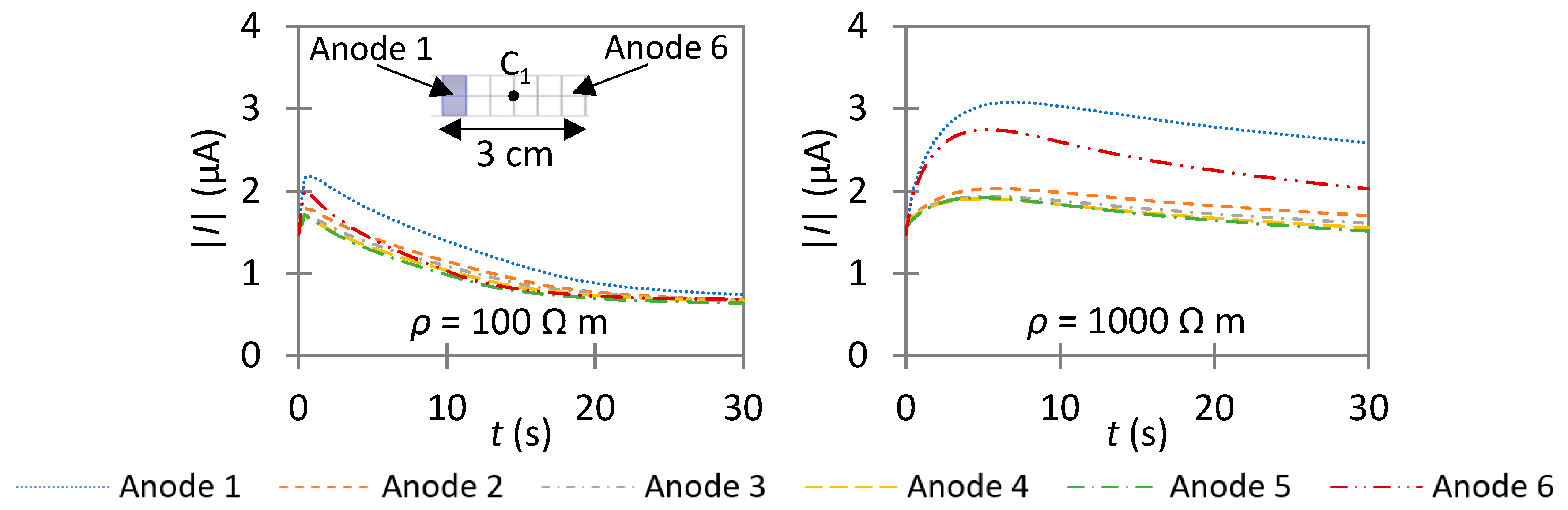
- The effect of the anode differs depending on its position relative to the monitoring device. It was shown that (i) corroding areas can mainly be located when they are below or in the vicinity of the current electrodes, and (ii) the area below the center of the device is almost not polarized irrespective of concrete resistivity. Hence, by adjusting the probe spacing, highly corroding areas will be either detected or not, depending on their position. This specificity should be helpful for estimating the position and length of highly corroding areas, which is one of the main problems when making any measurements on RC structures.
Supplementary Materials
Author Contributions
Funding
Acknowledgments
Conflicts of Interest
References
- Angst, U.M. Challenges and opportunities in corrosion of steel in concrete. Mater. Struct. 2018, 51, 4. [Google Scholar] [CrossRef] [Green Version]
- Rodrigues, R.; Gaboreau, S.; Gance, J.; Ignatiadis, I.; Betelu, S. Reinforced concrete structures: A review of corrosion mechanisms and advances in electrical methods for corrosion monitoring. Constr. Build. Mater. 2021, 121240. [Google Scholar] [CrossRef]
- Ahmad, S. Reinforcement corrosion in concrete structures, its monitoring and service life prediction—A review. Cem. Concr. Compos. 2003, 25, 459–471. [Google Scholar] [CrossRef]
- Nasser, A.; Clément, A.; Laurens, S.; Castel, A. Influence of steel—Concrete interface condition on galvanic corrosion currents in carbonated concrete. Corros. Sci. 2010, 52, 2878–2890. [Google Scholar] [CrossRef]
- Sohail, M.G.; Laurens, S.; Deby, F.; Balayssac, J.P. Significance of macrocell corrosion of reinforcing steel in partially carbonated concrete: Numerical and experimental investigation. Mater. Struct. 2015, 48, 217–233. [Google Scholar] [CrossRef]
- Warkus, J.; Raupach, M. Modelling of reinforcement corrosion—Geometrical effects on macrocell corrosion. Mater. Corros. 2009, 61, 494–504. [Google Scholar] [CrossRef]
- González, J.A.; Molina, A.; Escudero, M.L.; Andrade, C. Errors in the electrochemical evaluation of very small corrosion rates—I. Polarization resistance method applied to corrosion of steel in concrete. Corros. Sci. 1985, 25, 917–930. [Google Scholar] [CrossRef]
- Pereira, E.V.; Salta, M.M.; Fonseca, I.T.E. On the measurement of the polarisation resistance of reinforcing steel with embedded sensors: A comparative study. Mater. Corros. 2015, 66, 1029–1038. [Google Scholar] [CrossRef]
- Fahim, A.; Ghods, P.; Isgor, O.B.; Thomas, M.D.A. A critical examination of corrosion rate measurement techniques applied to reinforcing steel in concrete. Mater. Corros. 2018, 69, 1784–1799. [Google Scholar] [CrossRef]
- Stern, M.; Geary, A.L. Electrochemical polarization. J. Electrochem. Soc. 1957, 104, 56. [Google Scholar] [CrossRef]
- Angst, U.; Büchler, M. On the applicability of the Stern-Geary relationship to determine instantaneous corrosion rates in macro-cell corrosion. Mater. Corros. 2015, 66, 1017–1028. [Google Scholar] [CrossRef]
- Angst, U.; Büchler, M. A new perspective on measuring the corrosion rate of localized corrosion. Mater. Corros. 2020, 71, 808–823. [Google Scholar] [CrossRef]
- Wojtas, H. Determination of corrosion rate of reinforcement with a modulated guard ring electrode; analysis of errors due to lateral current distribution. Corros. Sci. 2004, 46, 1621–1632. [Google Scholar] [CrossRef]
- Feliu, S.; González, J.A.; Miranda, J.M.; Feliu, V. Possibilities and problems of in situ techniques for measuring steel corrosion rates in large reinforced concrete structures. Corros. Sci. 2005, 47, 217–238. [Google Scholar] [CrossRef]
- Poursaee, A.; Hansson, C.M. Galvanostatic pulse technique with the current confinement guard ring: The laboratory and finite element analysis. Corros. Sci. 2008, 50, 2739–2746. [Google Scholar] [CrossRef]
- Nygaard, P.V.; Geiker, M.R.; Elsener, B. Corrosion rate of steel in concrete: Evaluation of confinement techniques for on-site corrosion rate measurements. Mater. Struct. 2009, 42, 1059–1076. [Google Scholar] [CrossRef]
- Clément, A.; Laurens, S.; Arliguie, G.; Deby, F. Numerical study of the linear polarisation resistance technique applied to reinforced concrete for corrosion assessment. Eur. J. Environ. Civ. Eng. 2012, 16, 491–504. [Google Scholar] [CrossRef]
- Laurens, S.; Hénocq, P.; Rouleau, N.; Deby, F.; Samson, E.; Marchand, J.; Bissonnette, B. Steady-State polarization response of chloride-induced macrocell corrosion systems in steel reinforced concrete—Numerical and experimental investigations. Cem. Concr. Res. 2016, 79, 272–290. [Google Scholar] [CrossRef]
- Gepraegs, O.; Hansson, C. A comparative evaluation of three commercial unstruments for field measurements of reinforcing steel corrosion rates. J. ASTM Int. 2005, 2. [Google Scholar] [CrossRef]
- Monteiro, P.J.M.; Morrison, F.; Frangos, W. Non-Destructive measurement of corrosion state of reinforcing steel in concrete. ACI Mater. J. 1998, 95, 704–709. [Google Scholar] [CrossRef]
- Zhang, J.; Monteiro, P.J.M.; Morrison, H.F. Experimental and theoretical study of reinforced concrete corrosion using impedance measurements. Long Term Durab. Struct. Mater. 2001, 71–84. [Google Scholar] [CrossRef]
- Zhang, J.; Monteiro, P.J.M.; Morrison, H.F. Noninvasive surface measurement of corrosion impedance of reinforcing bar in concrete—Part 1: Experimental results. ACI Mater. J. 2001, 98, 116–125. [Google Scholar] [CrossRef]
- Zhang, J.; Monteiro, P.J.M.; Morrison, H.F. Noninvasive surface measurement of corrosion impedance of reinforcing bar in concrete—Part 2: Forward modeling. ACI Mater. J. 2002, 99, 242–249. [Google Scholar] [CrossRef]
- Hubbard, S.S.; Zhang, J.; Monteiro, P.J.M.; Peterson, J.E.; Rubin, Y. Experimental detection of reinforcing bar corrosion using nondestructive geophysical techniques. ACI Mater. J. 2003, 100, 501–510. [Google Scholar] [CrossRef]
- Zhang, J.; Monteiro, P.J.M.; Morrison, H.F.; Mancio, M. Noninvasive surface measurement of corrosion impedance of reinforcing bar in concrete—Part 3: Effect of geometry and material properties. ACI Mater. J. 2004, 101, 273–280. [Google Scholar]
- Keddam, M.; Nóvoa, X.R.; Vivier, V. The concept of floating electrode for contact-less electrochemical measurements: Application to reinforcing steel-bar corrosion in concrete. Corros. Sci. 2009, 51, 1795–1801. [Google Scholar] [CrossRef]
- Keddam, M.; Nóvoa, X.R.; Puga, B.; Vivier, V. Impedance based method for non-contact determination of the corrosion rate in buried metallic structures. Eur. J. Environ. Civ. Eng. 2011, 15, 1097–1103. [Google Scholar] [CrossRef]
- Lim, Y.-C.; Noguchi, T.; Shin, S.-W. Formulation of a nondestructive technique for evaluating steel corrosion in concrete structures. ISIJ Int. 2009, 49, 275–283. [Google Scholar] [CrossRef] [Green Version]
- Lim, Y.-C.; Noguchi, T.; Shin, S. Corrosion evaluation by estimating the surface resistivity of reinforcing bar. J. Adv. Concr. Technol. 2010, 8, 113–119. [Google Scholar] [CrossRef]
- Yu, J.; Sasamoto, A.; Iwata, M. Wenner method of impedance measurement for health evaluation of reinforced concrete structures. Constr. Build. Mater. 2019, 197, 576–586. [Google Scholar] [CrossRef]
- Alexander, C.L.; Orazem, M.E. Indirect electrochemical impedance spectroscopy for corrosion detection in external post-tensioned tendons: 1. Proof of concept. Corros. Sci. 2020, 164, 108331. [Google Scholar] [CrossRef]
- Alexander, C.L.; Orazem, M.E. Indirect impedance for corrosion detection of external post-tensioned tendons: 2. Multiple steel strands. Corros. Sci. 2020, 164, 108330. [Google Scholar] [CrossRef]
- Andrade, C.; Martínez, I.; Castellote, M. Feasibility of determining corrosion rates by means of stray current-induced polarisation. J. Appl. Electrochem. 2008, 38, 1467–1476. [Google Scholar] [CrossRef]
- Andrade, C.; Sanchez, J.; Martinez, I.; Rebolledo, N. Analogue circuit of the inductive polarization resistance. Electrochimica Acta 2011, 56, 1874–1880. [Google Scholar] [CrossRef]
- Fahim, A.; Ghods, P.; Alizaded, R.; Salehi, M.; Decarufel, S. CEPRA: A new test method for rebar corrosion rate measurement. Adv. Electrochem. Tech. Corros. Monit. Lab. Corros. Meas. 2019, STP1609, 59–80. [Google Scholar] [CrossRef]
- Warkus, J.; Raupach, M.; Gulikers, J. Numerical modelling of corrosion—Theoretical backgrounds. Mater. Corros. 2006, 57, 614–617. [Google Scholar] [CrossRef]
- Warkus, J.; Raupach, M. Modelling of reinforcement corrosion—Corrosion with extensive cathodes. Mater. Corros. 2006, 57, 920–925. [Google Scholar] [CrossRef]
- Otieno, M.B.; Beushausen, H.D.; Alexander, M.G. Modelling corrosion propagation in reinforced concrete structures—A critical review. Cem. Concr. Compos. 2011, 33, 240–245. [Google Scholar] [CrossRef]
- Isgor, O.B.; Razaqpur, A.G. Modelling steel corrosion in concrete structures. Mater. Struct. 2006, 39, 291–302. [Google Scholar] [CrossRef]
- Chalhoub, C.; François, R.; Garcia, D.; Laurens, S.; Carcasses, M. Macrocell corrosion of steel in concrete: Characterization of anodic behavior in relation to the chloride content. Mater. Corros. 2020. [Google Scholar] [CrossRef]
- Ožbolt, J.; Oršanić, F.; Balabanić, G.; Kušter, M. Modeling damage in concrete caused by corrosion of reinforcement: Coupled 3D FE model. Int. J. Fract. 2012, 178, 233–244. [Google Scholar] [CrossRef]
- Samson, G.; Deby, F.; Garciaz, J.-L.; Lassoued, M. An alternative method to measure corrosion rate of reinforced concrete structures. Cem. Concr. Compos. 2020, 112, 103672. [Google Scholar] [CrossRef]
- Fahim, A. Corrosion of Reinforcing Steel in Concrete: Monitoring Techniques and Mitigation Strategies. Master’s Thesis, University of New Brunswick, Fredericton, NB, Canada, 2018. [Google Scholar]
- Ožbolt, J.; Balabanić, G.; Kušter, M. 3D numerical modelling of steel corrosion in concrete structures. Corros. Sci. 2011, 53, 4166–4177. [Google Scholar] [CrossRef]
- Hu, X.; Shi, C.; Liu, X.; Zhang, J.; de Schutter, G. A review on microstructural characterization of cement-based materials by AC impedance spectroscopy. Cem. Concr. Compos. 2019, 100, 1–14. [Google Scholar] [CrossRef]
- Leroy, P.; Hördt, A.; Gaboreau, S.; Zimmermann, E.; Claret, F.; Bücker, M.; Stebner, H.; Huisman, J.A. Spectral induced polarization of low-pH cement and concrete. Cem. Concr. Compos. 2019, 104, 103397. [Google Scholar] [CrossRef]
- Khajehnouri, Y.; Chouteau, M.; Rivard, P.; Bérubé, C.L. Measuring electrical properties of mortar and concrete samples using the spectral induced polarization method: Laboratory set-up. Constr. Build. Mater. 2019, 210, 1–12. [Google Scholar] [CrossRef]
- Ge, J.; Isgor, O.B. Effects of Tafel slope, exchange current density and electrode potential on the corrosion of steel in concrete. Mater. Corros. 2007, 58, 573–582. [Google Scholar] [CrossRef]
- Duprat, F.; Larrard, T.; Vu, N.T. Quantification of Tafel coefficients according to passive/active state of steel carbonation-induced corrosion in concrete. Mater. Corros. 2019, 70, 1934–1963. [Google Scholar] [CrossRef]
- Stefanoni, M.; Angst, U.M.; Elsener, B. Electrochemistry and capillary condensation theory reveal the mechanism of corrosion in dense porous media. Sci. Rep. 2018, 8, 7407. [Google Scholar] [CrossRef] [Green Version]
- Stefanoni, M.; Angst, U.M.; Elsener, B. Kinetics of electrochemical dissolution of metals in porous media. Nat. Mater. 2019, 18, 942–947. [Google Scholar] [CrossRef] [Green Version]
- Ji, Y.; Wu, M.; Tan, Z.; Gao, F.; Liu, F. Process control of reinforcement corrosion in concrete. Part 2: Time-Dependent dominating factors under different environmental conditions. Constr. Build. Mater. 2014, 73, 214–221. [Google Scholar] [CrossRef]
- Ji, Y.; Zhan, G.; Tan, Z.; Hu, Y.; Gao, F. Process control of reinforcement corrosion in concrete. Part 1: Effect of corrosion products. Constr. Build. Mater. 2015, 79, 214–222. [Google Scholar] [CrossRef]
- Andrade, C.; Alonso, C.; Gulikers, J.; Polder, R.; Cigna, R.; Vennesland, Ø.; Salta, M.; Raharinaivo, A.; Elsener, B. Test methods for on-site corrosion rate measurement of steel reinforcement in concrete by means of the polarization resistance method. Mater. Struct. 2004, 37, 623–642. [Google Scholar] [CrossRef]
- Stefanoni, M.; Angst, U.; Elsener, B. Corrosion rate of carbon steel in carbonated concrete—A critical review. Cem. Concr. Res. 2018, 103, 35–48. [Google Scholar] [CrossRef]
- Angst, U.M. Durable concrete structures: Cracks & corrosion and corrosion & cracks. In Proceedings of the 10th International Conference on Fracture Mechanics of Concrete and Concrete Structures (FraMCoS-X), Bayonne, France, 24–26 June 2019; pp. 1–10. [Google Scholar]
- Kranc, S.C.; Sagüés, A.A. Detailed modeling of corrosion macrocells on steel reinforcing in concrete. Corros. Sci. 2001, 43, 1355–1372. [Google Scholar] [CrossRef]
- Marchand, J.; Laurens, S.; Protière, Y.; Samson, E. A numerical study of polarization tests applied to corrosion in reinforced concrete. Spec. Publ. 2016, 312, 1–12. [Google Scholar]
- Chalhoub, C.; François, R.; Carcasses, M. Effect of cathode-anode distance and electrical resistivity on macrocell corrosion currents and cathodic response in cases of chloride induced corrosion in reinforced concrete structures. Constr. Build. Mater. 2020, 245, 118337. [Google Scholar] [CrossRef]
- Andrade, C.; Martínez, I. Techniques for measuring the corrosion rate (polarization resistance) and the corrosion potential of reinforced concrete structures. Non Destruct. Eval. Reinf. Concr. Struct. 2010, 284–316. [Google Scholar] [CrossRef]
- Hansson, C.M.; Poursaee, A.; Laurent, A. Macrocell and microcell corrosion of steel in ordinary Portland cement and high performance concretes. Cem. Concr. Res. 2006, 36, 2098–2102. [Google Scholar] [CrossRef]
- Poursaee, A.; Hansson, C.M. Potential pitfalls in assessing chloride-induced corrosion of steel in concrete. Cem. Concr. Res. 2009, 39, 391–400. [Google Scholar] [CrossRef]
- Revert, A.B.; Hornbostel, K.; De Weerdt, K.; Geiker, M.R. Macrocell corrosion in carbonated Portland and Portland-fly ash concrete—Contribution and mechanism. Cem. Concr. Res. 2019, 116, 273–283. [Google Scholar] [CrossRef] [Green Version]
- González, J.A.; Cobo, A.; González, M.N.; Feliu, S. On-Site determination of corrosion rate in reinforced concrete structures by use of galvanostatic pulses. Corros. Sci. 2001, 43, 611–625. [Google Scholar] [CrossRef]
- Glass, G.K.; Page, C.L.; Short, N.R.; Zhang, J.Z. The analysis of potentiostatic transients applied to the corrosion of steel in concrete. Corros. Sci. 1997, 39, 1657–1663. [Google Scholar] [CrossRef]
- Angst, U.M.; Elsener, B. On the applicability of Wenner method for resistivity measurements of concrete. ACI Mater. J. 2014, 111, 661–672. [Google Scholar] [CrossRef]
- Sengul, O.; Gjorv, O.E. Electrical resistivity measurements for quality control during concrete construction. ACI Mater. J. 2008, 105, 541–547. [Google Scholar] [CrossRef]
- Alhajj, M.A.; Palma-Lopes, S.; Villain, G. Accounting for steel rebar effect on resistivity profiles in view of reinforced concrete structure survey. Constr. Build. Mater. 2019, 223, 898–909. [Google Scholar] [CrossRef]
- Chen, C.-T.; Chang, J.-J.; Yeih, W. The effects of specimen parameters on the resistivity of concrete. Constr. Build. Mater. 2014, 71, 35–43. [Google Scholar] [CrossRef]
- Garzon, A.J.; Sanchez, J.; Andrade, C.; Rebolledo, N.; Menéndez, E.; Fullea, J. Modification of four point method to measure the concrete electrical resistivity in presence of reinforcing bars. Cem. Concr. Compos. 2014, 53, 249–257. [Google Scholar] [CrossRef]
- François, R.; Laurens, S.; Deby, F. Steel Corrosion in Reinforced Concrete. In Corrosion and Its Consequences for Reinforced Concrete Structures; Elsevier: London, UK, 2018; pp. 1–41. ISBN 978-1-78548-234-2. [Google Scholar]
- Angst, U.M.; Geiker, M.R.; Michel, A.; Gehlen, C.; Wong, H.; Isgor, O.B.; Elsener, B.; Hansson, C.M.; François, R.; Hornbostel, K.; et al. The steel-concrete interface. Mater. Struct. 2017, 50, 143. [Google Scholar] [CrossRef]
- Angst, U.M.; Geiker, M.R.; Alonso, M.C.; Polder, R.; Isgor, O.B.; Elsener, B.; Wong, H.; Michel, A.; Hornbostel, K.; Gehlen, C.; et al. The effect of the steel-concrete interface on chloride-induced corrosion initiation in concrete: A critical review by RILEM TC 262-SCI. Mater. Struct. 2019, 52, 88. [Google Scholar] [CrossRef]
- Hornbostel, K.; Elsener, B.; Angst, U.M.; Larsen, C.K.; Geiker, M.R. Limitations of the use of concrete bulk resistivity as an indicator for the rate of chloride-induced macro-cell corrosion. Struct. Concr. 2017, 18, 326–333. [Google Scholar] [CrossRef] [Green Version]
- Sadowski, Ł. New non-destructive method for linear polarisation resistance corrosion rate measurement. Arch. Civ. Mech. Eng. 2010, 10, 109–116. [Google Scholar] [CrossRef]
- Azarsa, P.; Gupta, R. Electrical resistivity of concrete for durability evaluation: A review. Adv. Mater. Sci. Eng. 2017, 2017, 8453095. [Google Scholar] [CrossRef] [Green Version]
- Gowers, K.R.; Millard, S.G. Measurement of concrete resistivity for assessment of corrosion severity of steel using Wenner technique. ACI Mater. J. 1999, 96, 536–541. [Google Scholar] [CrossRef]
- Sengul, O.; Gjorv, O.E. Effect of embedded steel on electrical resistivity measurements on concrete structures. ACI Mater. J. 2009, 106, 11–18. [Google Scholar] [CrossRef]
- Presuel-Moreno, F.; Liu, Y.; Wu, Y.-Y. Numerical modeling of the effects of rebar presence and/or multilayered concrete resistivity on the apparent resistivity measured via the Wenner method. Constr. Build. Mater. 2013, 48, 16–25. [Google Scholar] [CrossRef]
- Salehi, M.; Ghods, P.; Burkan Isgor, O. Numerical investigation of the role of embedded reinforcement mesh on electrical resistivity measurements of concrete using the Wenner probe technique. Mater. Struct. 2016, 49, 301–316. [Google Scholar] [CrossRef]
- Nguyen, A.Q.; Klysz, G.; Deby, F.; Balayssac, J.-P. Evaluation of water content gradient using a new configuration of linear array four-point probe for electrical resistivity measurement. Cem. Concr. Compos. 2017, 83, 308–322. [Google Scholar] [CrossRef]
- Ghosh, P.; Tran, Q. Influence of parameters on surface resistivity of concrete. Cem. Concr. Compos. 2015, 62, 134–145. [Google Scholar] [CrossRef]
- Lim, Y.C.; Kim, T.S.; Hwang, C.S. Modeling for apparent resistivity estimation along direction of electrode array above rebar in electrical resistivity measurement. J. Build. Eng. 2020, 31, 101417. [Google Scholar] [CrossRef]
- Nguyen, A.Q.; Klysz, G.; Deby, F.; Balayssac, J.P. Assessment of the electrochemical state of steel reinforcement in water saturated concrete by resistivity measurement. Constr. Build. Mater. 2018, 171, 455–466. [Google Scholar] [CrossRef]
- Elsener, B.; Andrade, C.; Gulikers, J.; Polder, R.; Raupach, M. Half-cell potential measurements—Potential mapping on reinforced concrete structures. Mater. Struct. 2003, 36, 461–671. [Google Scholar] [CrossRef]
- Orazem, M.E.; Tribollet, B. Electrochemical Impedance Spectroscopy; John Wiley & Sons: Hoboken, NJ, USA, 2011; ISBN 111820994X. [Google Scholar]
- Chakri, S.; Frateur, I.; Orazem, M.E.; Sutter, E.M.M.; Tran, T.T.M.; Tribollet, B.; Vivier, V. Improved EIS analysis of the electrochemical behaviour of carbon steel in alkaline solution. Electrochimica Acta 2017, 246, 924–930. [Google Scholar] [CrossRef]
- Nguyen, W.; Duncan, J.F.; Devine, T.M.; Ostertag, C.P. Electrochemical polarization and impedance of reinforced concrete and hybrid fiber-reinforced concrete under cracked matrix conditions. Electrochimica Acta 2018, 271, 319–336. [Google Scholar] [CrossRef] [Green Version]
- Yu, B.; Yang, L.; Wu, M.; Li, B. Practical model for predicting corrosion rate of steel reinforcement in concrete structures. Constr. Build. Mater. 2014, 54, 385–401. [Google Scholar] [CrossRef]
- Wai-Lok Lai, W.; Dérobert, X.; Annan, P. A review of ground penetrating radar application in civil engineering: A 30-year journey from locating and testing to imaging and diagnosis. NDT E Int. 2018, 96, 58–78. [Google Scholar] [CrossRef]
- Tosti, F.; Ferrante, C. Using ground penetrating radar methods to investigate reinforced concrete structures. Surv. Geophys. 2019, 1–46. [Google Scholar] [CrossRef]
- Zhou, F.; Chen, Z.; Liu, H.; Cui, J.; Spencer, B.; Fang, G. Simultaneous estimation of rebar diameter and cover thickness by a GPR-EMI dual sensor. Sensors 2018, 18, 2969. [Google Scholar] [CrossRef] [Green Version]
- Sadowski, L. Methodology for assessing the probability of corrosion in concrete structures on the basis of half-cell potential and concrete resistivity measurements. Sci. World J. 2013, 2013, 714501. [Google Scholar] [CrossRef] [Green Version]
- Kušter Marić, M.; Mandić Vlašić, A.; Ivanković, A.M.; Bleiziffer, J.; Srbić, M.; Skokandić, D. Assessment of reinforcement corrosion and concrete damage on bridges using non-destructive testing. Gradjevinar 2019, 71, 843–862. [Google Scholar] [CrossRef]
- Andrade, C. Electrochemical methods for on-site corrosion detection. Struct. Concr. 2020, 21, 1385–1395. [Google Scholar] [CrossRef]
- Karhunen, K.; Seppänen, A.; Lehikoinen, A.; Monteiro, P.J.M.; Kaipio, J.P. Electrical resistance tomography imaging of concrete. Cem. Concr. Res. 2010, 40, 137–145. [Google Scholar] [CrossRef]
- Reichling, K.; Raupach, M.; Klitzsch, N. Determination of the distribution of electrical resistivity in reinforced concrete structures using electrical resistivity tomography. Mater. Corros. 2015, 66, 763–771. [Google Scholar] [CrossRef]
- Smyl, D. Electrical tomography for characterizing transport properties in cement-based materials: A review. Constr. Build. Mater. 2020, 244, 118299. [Google Scholar] [CrossRef]
- Smyl, D.; Hallaji, M.; Seppänen, A.; Pour-Ghaz, M. Quantitative electrical imaging of three-dimensional moisture flow in cement-based materials. Int. J. Heat Mass Transf. 2016, 103, 1348–1358. [Google Scholar] [CrossRef] [Green Version]
- Smyl, D.; Rashetnia, R.; Seppänen, A.; Pour-Ghaz, M. Can electrical resistance tomography be used for imaging unsaturated moisture flow in cement-based materials with discrete cracks? Cem. Concr. Res. 2017, 91, 61–72. [Google Scholar] [CrossRef] [Green Version]
- Fares, M.; Villain, G.; Bonnet, S.; Palma Lopes, S.; Thauvin, B.; Thiery, M. Determining chloride content profiles in concrete using an electrical resistivity tomography device. Cem. Concr. Compos. 2018, 94, 315–326. [Google Scholar] [CrossRef] [Green Version]
- Bonnet, S.; Balayssac, J.-P. Combination of the Wenner resistivimeter and Torrent permeameter methods for assessing carbonation depth and saturation level of concrete. Constr. Build. Mater. 2018, 188, 1149–1165. [Google Scholar] [CrossRef] [Green Version]
- Rymarczyk, T.; Kłosowski, G.; Kozłowski, E. A Non-Destructive System Based on Electrical Tomography and Machine Learning to Analyze the Moisture of Buildings. Sensors 2018, 18, 2285. [Google Scholar] [CrossRef] [Green Version]
- Loke, M.H. Tutorial: 2-D and 3-D Electrical Imaging Surveys; Geotomo Software: Penang, Malaysia, 2004. [Google Scholar]
- Udosen, N.; Potthast, R. Automated optimization of electrode locations for electrical resistivity tomography. Model. Earth Syst. Environ. 2018, 4, 1059–1083. [Google Scholar] [CrossRef]
- Smyl, D.; Liu, D. Optimizing electrode positions in 2D Electrical Impedance Tomography using deep learning. IEEE Trans. Instrum. Meas. 2020, 69, 6030–6044. [Google Scholar] [CrossRef] [Green Version]


| Active Area (Anode) | Passive Area (Cathode) | References | ||||||
|---|---|---|---|---|---|---|---|---|
| i0,a (A m−2) | Eeq,a (V) | βa,a (V) | βc,a (V) | i0,c (A m−2) | Eeq,c (V) | βa,c (V) | βc,c (V) | |
| 1.875 × 10⁻⁴ | −0.78 | 0.06 | - | 6.25 × 10⁻⁶ | 0.16 | - | 0.16 | [44,57] |
| 3 × 10⁻⁴ | −0.78 | 0.09 | 0.18 | 10−5 | 0.16 | 5 | 0.18 | [43] |
| 5 × 10⁻³ | −0.65 | 0.09 | 0.15 | 2.5 × 10⁻⁴ | −0.15 | 0.4 | 0.15 | [5] |
| 0.1 | −0.7 | 0.06 | 0.16 | 10−4 | −0.1 | 0.4 | 0.16 | [18,58] |
| 0.3 | −0.576 | 0.046 | 0.3 | 6 × 10⁻⁵ | −0.11 | 0.24 | 0.3 | [59] |
| Active Corrosion | Passive Corrosion | ||||||
|---|---|---|---|---|---|---|---|
| i0,a (A m−2) | Eeq,a (V) | αa,a (V) | αc,a (V) | i0,c (A m−2) | Eeq,c (V) | αa,c (V) | αc,c (V) |
| 0.1 | 0 | 0.5 | 0.5 | - | - | - | - |
| - | - | - | - | 10−5 | 0 | 0.012 | 0.5 |
| 0.1 or 10−4 | 0 | 0.5 | 0.5 | 10−5 | 0 | 0.012 | 0.5 |
| a (cm) | kWenner = 2πa (m) | kCOMSOL (m) |
|---|---|---|
| 2.5 | 0.157 | 0.149 |
| 5 | 0.314 | 0.304 |
| 7.5 | 0.471 | 0.387 |
| 10 | 0.628 | 0.424 |
| 15 | 0.942 | 0.405 |
| Input Parameters | Values |
|---|---|
| Current impressed on C1 IC1 (µA) | 100, 300 or 500 |
| Concrete resistivity ρ (Ω m) | 100, 200, 500 or 1000 |
| Probe spacing a (cm) | 2.5, 5, 7.5, 10 or 15 |
| Cover depth e (mm) | 20, 40 or 60 |
| Rebar diameter Φ (mm) | 6, 12 or 25 |
| Input Parameters | Values |
|---|---|
| Current impressed on C1 IC1 (µA) | 100 |
| Concrete resistivity ρ (Ω m) | 100, 200, 500 or 1000 |
| Anode length La (cm) | 1 or 3 (5, 7.5, 10, or 15 in SI) |
| Probe spacing a (cm) | 2.5, 5 or 15 |
| Cover depth e (mm) | 40 |
| Rebar diameter Φ (mm) | 12 |
| Double-layer capacitance Cdl (F m−2) | 0.2 or 2 |
Publisher’s Note: MDPI stays neutral with regard to jurisdictional claims in published maps and institutional affiliations. |
© 2020 by the authors. Licensee MDPI, Basel, Switzerland. This article is an open access article distributed under the terms and conditions of the Creative Commons Attribution (CC BY) license (http://creativecommons.org/licenses/by/4.0/).
Share and Cite
Rodrigues, R.; Gaboreau, S.; Gance, J.; Ignatiadis, I.; Betelu, S. Indirect Galvanostatic Pulse in Wenner Configuration: Numerical Insights into Its Physical Aspect and Its Ability to Locate Highly Corroding Areas in Macrocell Corrosion of Steel in Concrete. Corros. Mater. Degrad. 2020, 1, 373-407. https://0-doi-org.brum.beds.ac.uk/10.3390/cmd1030018
Rodrigues R, Gaboreau S, Gance J, Ignatiadis I, Betelu S. Indirect Galvanostatic Pulse in Wenner Configuration: Numerical Insights into Its Physical Aspect and Its Ability to Locate Highly Corroding Areas in Macrocell Corrosion of Steel in Concrete. Corrosion and Materials Degradation. 2020; 1(3):373-407. https://0-doi-org.brum.beds.ac.uk/10.3390/cmd1030018
Chicago/Turabian StyleRodrigues, Romain, Stéphane Gaboreau, Julien Gance, Ioannis Ignatiadis, and Stéphanie Betelu. 2020. "Indirect Galvanostatic Pulse in Wenner Configuration: Numerical Insights into Its Physical Aspect and Its Ability to Locate Highly Corroding Areas in Macrocell Corrosion of Steel in Concrete" Corrosion and Materials Degradation 1, no. 3: 373-407. https://0-doi-org.brum.beds.ac.uk/10.3390/cmd1030018