
Differentiation of SCC Susceptibility with EIS of Alloy 182 in High Temperature Water

SCK CEN (Belgian Nuclear Research Centre), Boeretang 200, B-2400 Mol, Belgium
*
Author to whom correspondence should be addressed.
Corros. Mater. Degrad. 2021, 2(3), 341-359; https://0-doi-org.brum.beds.ac.uk/10.3390/cmd2030018
Submission received: 15 April 2021
/
Revised: 2 June 2021
/
Accepted: 16 June 2021
/
Published: 24 June 2021
(This article belongs to the Special Issue Corrosion and Protection of Metals and Alloys in the Energy and Carbon Abatement Sectors: Arduous and Extreme Environments)
Abstract
:Electrochemical Impedance Spectroscopy (EIS) measurements were carried out in high temperature water with Ni-based Alloy-182. The aim was to correlate the EIS results with differences in Stress Corrosion Cracking (SCC) susceptibility that is present around the Ni-NiO transition. There was a clear difference between the EIS results at and away from the Ni-NiO transition. To make a more quantitative correlation a simple equivalent circuit was used to fit the experimental data. A clear correlation between the CPE exponent (n) and the SCC susceptibility could be obtained. Additionally, it was shown that the high frequency arc of the EIS data was related to the diffuse double layer
1. Introduction
Due to the ability of nickel-based alloys to offer good mechanical properties, corrosion resistance and compatibility to other materials, they are frequently used as a weld metal for internal components of Pressurized Water Reactors (PWR). For instance, the nickel-based Alloy 182 is commonly used as a weld material between a low-alloy steel component, e.g., a nozzle made of SA 508, and a stainless steel component, e.g., a pipe made of 316 L. Alloy 182 is known to accommodate the differences in composition and thermal expansion of the two connecting metals [1,2]. However, Alloy 182 is prone to primary water stress corrosion cracking (PWSCC) in the PWRs primary circuit [2]. As such, the stress corrosion cracking behavior of this alloy has been investigated quite extensively [1,2,3,4,5,6,7,8].
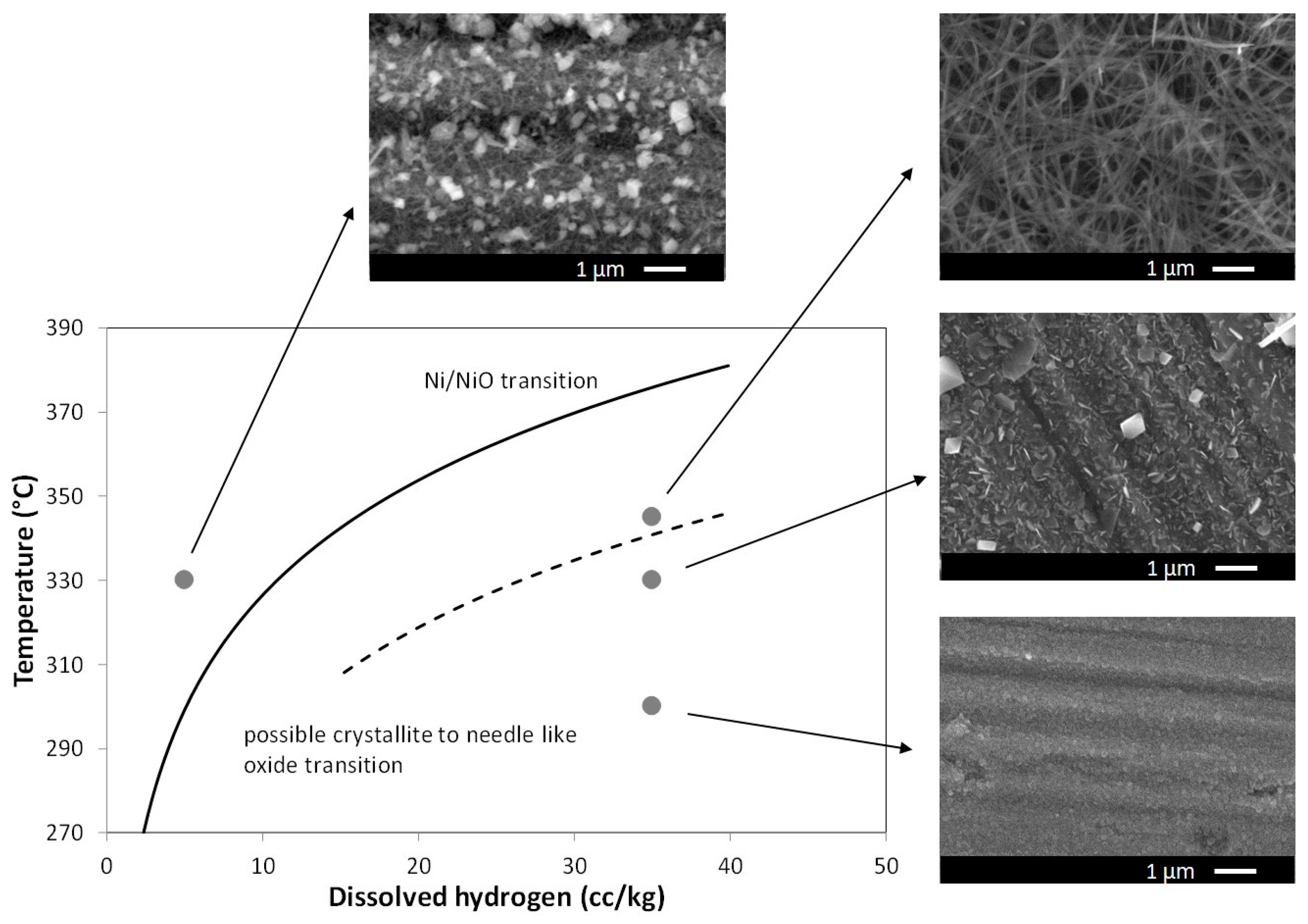
Nickel-based alloys, like Alloy 182, show a maximum in SCC crack growth around certain combinations of dissolved hydrogen content and temperature [3]. It is believed that this maximum in crack growth rate is related to the Ni/NiO transition [4]. The oxide film established on Alloy 182 in PWR water is thought to consist of two layers: a chromium-rich spinel layer growing into the metal and a deposited layer on top of it [5,6,7]. The character of the deposited layer, mainly containing nickel and iron, changes when crossing the Ni/NiO transition line from crystal-like magnetite or trevorite (in the Ni stability region) to needle-like nickel-oxide [8]. In previous work the oxide layers formed at different combinations of dissolved hydrogen and temperature were investigated [9]. It was shown that there are distinct differences in the oxide layer morphologies in various areas of the dissolved hydrogen–temperature space.
In this work we investigate whether in-situ Electrochemical Impedance Spectroscopy (EIS) measurements can be used to differentiate between these different oxide layer morphologies. EIS measurements are particularly suitable for in-situ measurements in high temperature water systems where a “pseudo” reference electrode could be used. This “pseudo” reference electrode can be made from platinum or even the same material as the test specimens. EIS measurements were carried out successfully on stainless steels and Ni-based Alloys in high temperature water to distinguish between the different materials and water chemistries [10,11]. Other than our work, only a few studies were carried out with EIS to investigate the oxidation behavior of Ni-based alloys 600, 690 and 182 in high temperature water [12,13,14,15,16,17]. Results with Alloy 182 show that the oxide layer morphology strongly depends on the temperature and dissolved hydrogen concentrations. The reported surface appearances could vary between rather smooth, crystallites shaped to needle like oxides with a very dispersed morphology. Similarly, EIS was used to study the oxidation behavior of stainless steel in super critical and high temperature water [18,19].
In this study we used the same approach as described in reference [9], where measurements were carried out at different combinations of dissolved hydrogen and temperature. This is illustrated in Figure 1 where the Ni-NiO transition curve is plotted as a function of temperature and dissolved hydrogen concentration, including the different oxide layer morphologies. The Ni-NiO transition curve is taken from Andresen (solid line) [3], based on recent experimental results and calculations and is situated above the Terachi curve (dashed line) [20], based on earlier, thermodynamic calculations. Notice that the Andresen curve was set using data published previously by Attanasio and Morton [4,20]. The dots show the test conditions where EIS measurements were carried out.
2. Materials and Methods
2.1. Materials
2.2. Environment
Tests were carried out under representative PWR primary water chemistry. Such a water chemistry consists of Boron (added to control reactivity), Lithiumhydroxide to control the pH and dissolved hydrogen to suppress radiolysis [21,22]. The temperatures and hydrogen concentrations were chosen in a way that they correspond to the test conditions as shown in Figure 1. Notice that a PWR is operated in the temperature range 300 to 345 °C and as such the materials used in the primary circuit are subjected to these temperatures as well. Boron was added as boric acid, H3BO3, with a concentration of 1000 ppm B. Lithium was added as lithium hydroxide with a concentration of 2 ppm Li. The resulting high temperature pH was calculated to be approximately 7.12. Hydrogen was added to the water by hydrogen purging at appropriate partial pressures to get the desired concentrations of dissolved hydrogen. The simulated PWR water was circulated through the autoclave at a rate of approximately 10 L per hour and the water chemistry was controlled by resin ion exchangers saturated with lithium and boron. The water in the recirculation loop was cooled to room temperature after passing through the autoclave and the conductivity, dissolved oxygen concentration, dissolved hydrogen concentration and pH were continuously monitored.
2.3. Electrode Set-Up
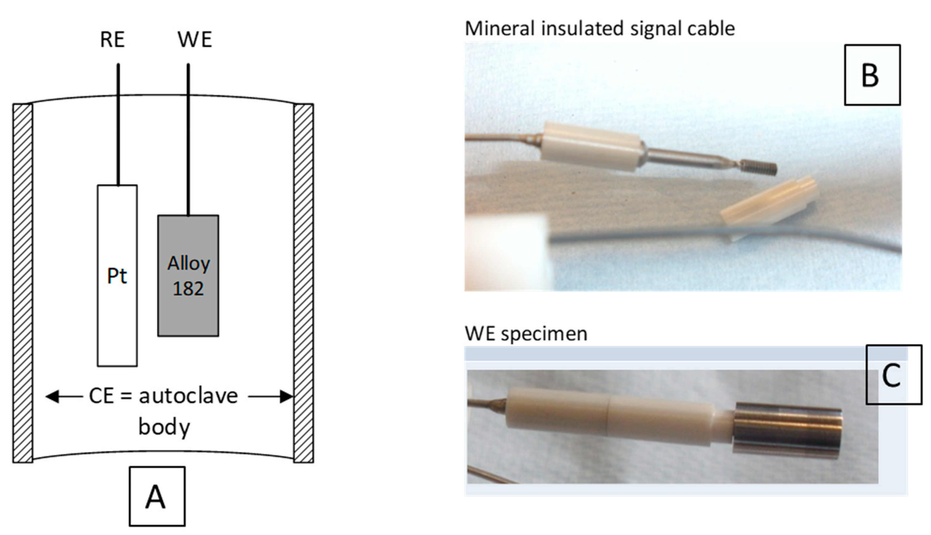
Figure 3 shows the electrode arrangement in the autoclave. The working electrode was positioned in the middle of the autoclave. A Pt rod served as a pseudo reference electrode for the high temperature impedance measurements. The test specimens were attached to a Thermocoax cable via a suitable connector and served as a working electrode (see Figure 3 right-hand side). This allowed to make electrochemical measurements up to 345 °C. The autoclave body served as the counter electrode, which guaranteed a uniform distribution of the currents and potentials of the electrochemical cell. The specimens were cylindrical in shape with a diameter of 5 mm and length of 10 mm, resulting in a surface area of 193 mm2. The surface finish was 1200 grit.
2.4. EIS Measurements
Electrochemical measurements were performed in an autoclave connected to a water recirculation loop that maintained a simulated primary water PWR environment. Electrochemical measurements were performed with a Gamry Instruments Reference 600 system (Warminster, PA, USA). The system had a floating earth and so could be used in autoclave systems. The total test time was two weeks with one EIS test per day. Before each test the open circuit potential (OCP) was measured during 5 min. Electrochemical impedance spectroscopy (EIS) was performed from 100 kHz down to 1 mHz with 10 points per decade and an amplitude of 10 mV around the OCP.
The test matrix is shown in Table 2. It shows the four test conditions that were used in this work. These test conditions correspond with different oxide layer morphologies as shown in Figure 1. The temperature and hydrogen concentrations were chosen such that they corresponded with the dot in Figure 1. Notice that a temperature variation of only 15 °C can result in a remarkable difference in oxide layer morphology (test condition 2 versus test condition 3).
3. Results
The EIS data were interpreted in two different ways. The first method was to fit the experimental data with an equivalent circuit to obtain different kinetic parameters that could describe the corrosion processes that took place at the metal-oxide-solution interface. The second method was to examine the low frequency impedances and compare these with the different measurements.
3.1. Equivalent Circuit Modelling
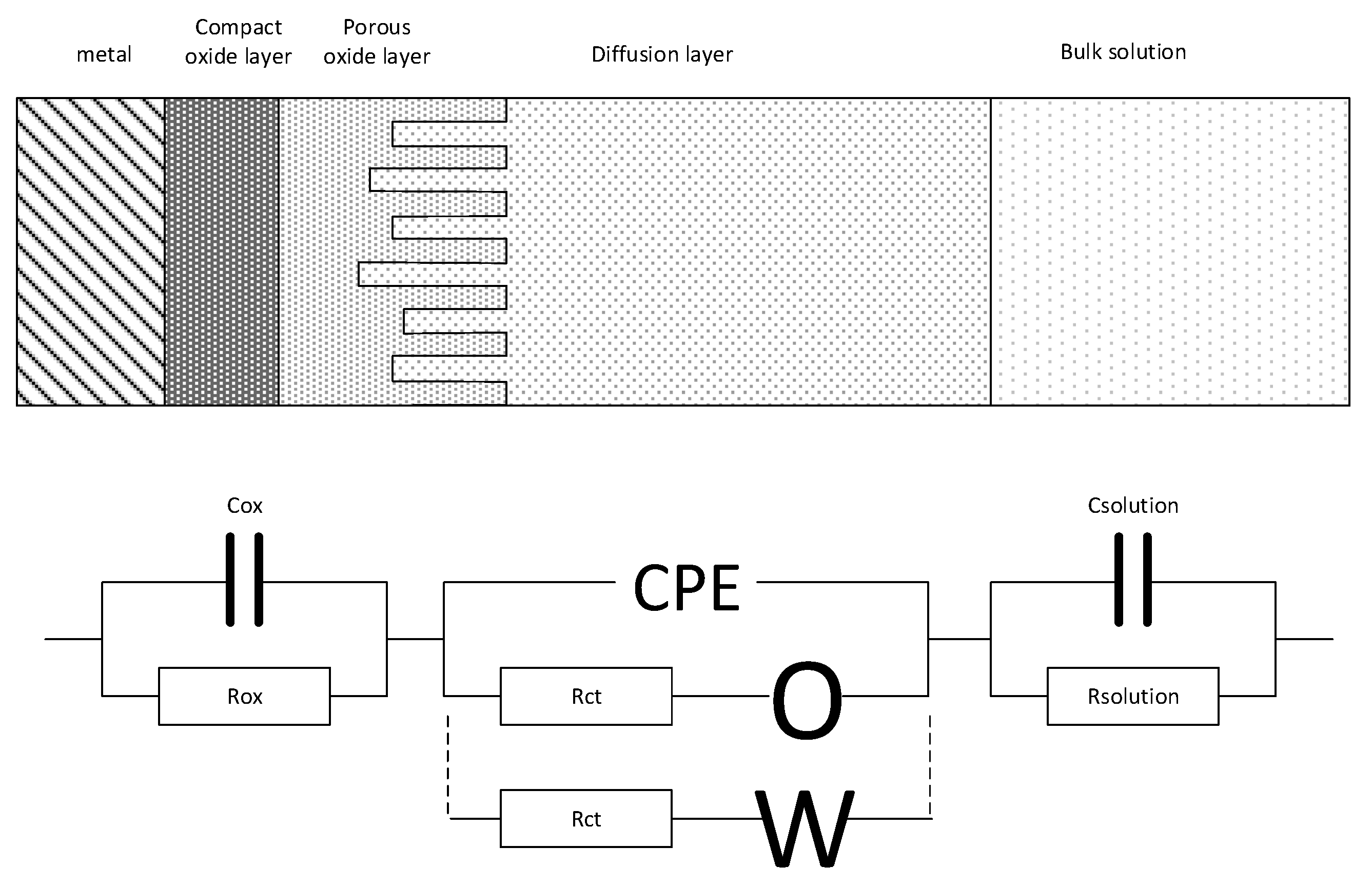
Several equivalent circuits are proposed to interpret high temperature impedance data on austenitic stainless steel materials [11,12,18]. These models all distinguish between a high frequency part typically related to the oxide layer, a mid-frequency part related to the electrochemical double layer and a charge transfer resistance, and finally a low frequency part related to diffusion effects. Based on these assumptions an equivalent circuit model was constructed as shown in Figure 4, with the main difference being that the capacity of the diffuse double layer was added. This model was used to interpret the experimental data. The equivalent circuit model consists of the following elements [23,24]:
- Cox: the capacity of the oxide layer, that is present on the metal surface
- Rox: the (ohmic) resistance of the oxide layer
- Rct: charge transfer resistance of the electrochemical reactions that take place at the oxide layer water interface
- O: diffusion resistance related to the electrochemical active species moving from and to the oxide layer water interface, assuming a finite length of the diffusion layer (first alternative). The impedance (ZO) is given by:where σ is the Warburg coefficient and B a Warburg fit parameter represented by B = δ/√D. Here δ is the diffusion layer thickness and D is some average value of the diffusion coefficients of the diffusion species.
- W: diffusion resistance related to electrochemical active species moving from and to the oxide layer water interface, assuming an infinite length of the diffusion layer (second alternative). The impedance (ZW) is given by:where σ is the Warburg coefficient.
- CPE: Constant Phase Element representing the electrochemical double layer capacity on a heterogeneous/dispersed substrate. The impedance is given by:where Yo is the CPE constant or pseudo capacitance and n the CPE exponent.
- Csolution: diffuse double layer capacity
- Rsolution: solution resistance of the test water
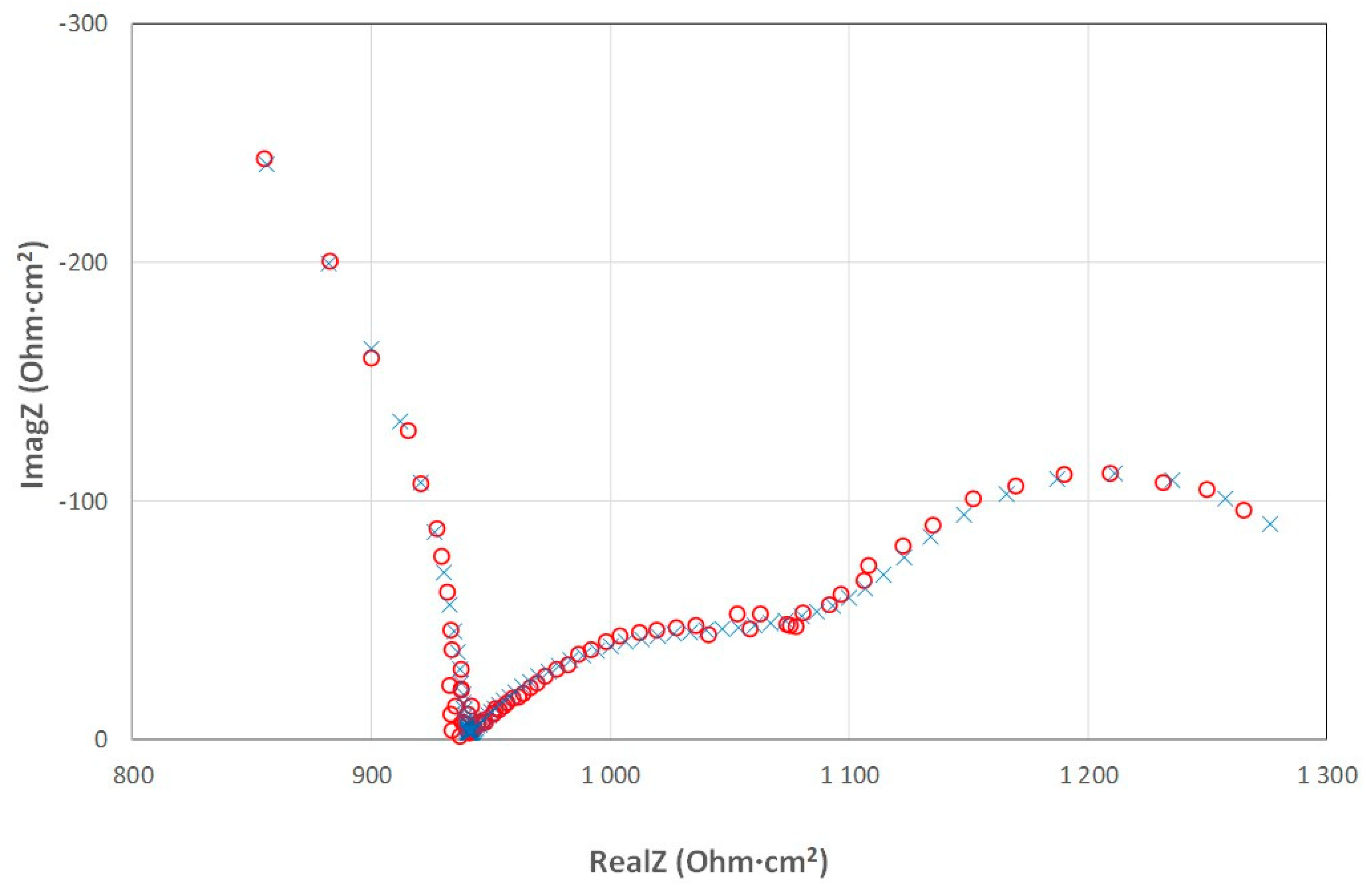
Figure 5 shows a fit example of the impedance data after eight days of testing at 300 °C with the equivalent circuit of Figure 4. This fit was performed for all the impedance data in order to observe trends in parameter values with time. The results are reported in Section 3.4.
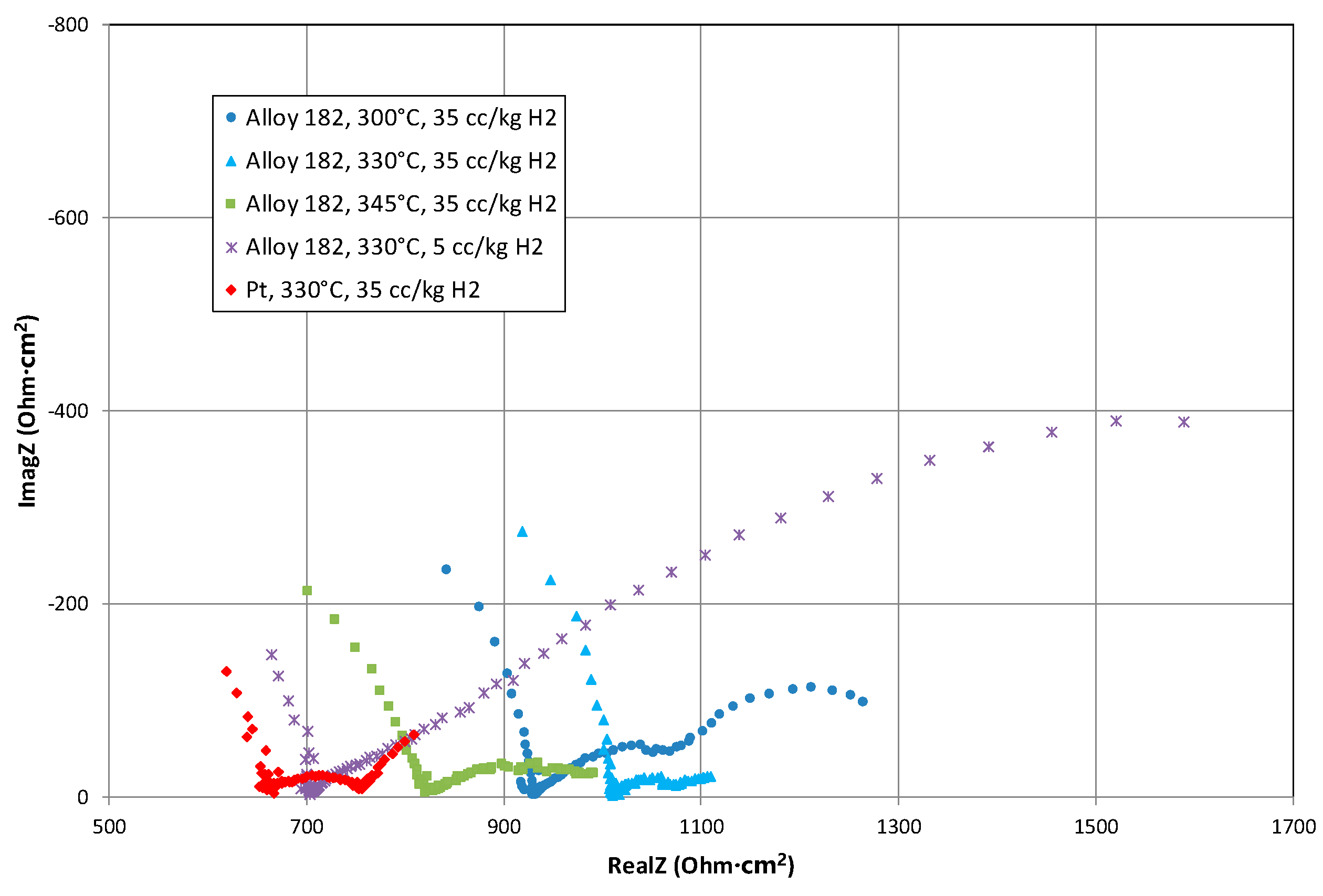
Figure 6 shows the impedance data after eight days of testing for the five test conditions. All the specimens, including the Pt electrode, exhibit a large high frequency arc. The origin of this arc will be discussed in Section 3.2. A first visual interpretation shows that at 35 cc/kg H2 the shape of the Nyquist plots are similar for the Pt and Alloy 182 electrodes, there is a decreasing part at the left, a central elliptical part and an increasing part at the right. Only the sizes (the actual values) are different. This means that the electrochemical response is dominated by the electrokinetic behavior of the dissolved hydrogen, which is in agreement with results from reference [11]. The impedance result of the low hydrogen concentration is clearly different in shape and size. That is, a higher impedance of the electrochemical reactions can be noticed, which is related to the lower hydrogen concentration. This in fact confirms again the dominance of the hydrogen oxidation/reduction reaction on the total impedance. The equivalent circuit fit results are shown in Table 3. The results of the high frequency arc are not mentioned in this table as they will be discussed in Section 3.2. The numbers in Table 3 confirm the visual observations. The highest Rct is found for the lowest hydrogen concentration (5 cc/kg). The lowest n value (which is a measure for the surface roughness/porosity) is found for the test condition, where the needle like oxide is present (35 cc/kg H2, and 345 °C). This surface is shown in Figure 1 and is highly irregular.
3.2. Interpretation of the High Frequency Arc
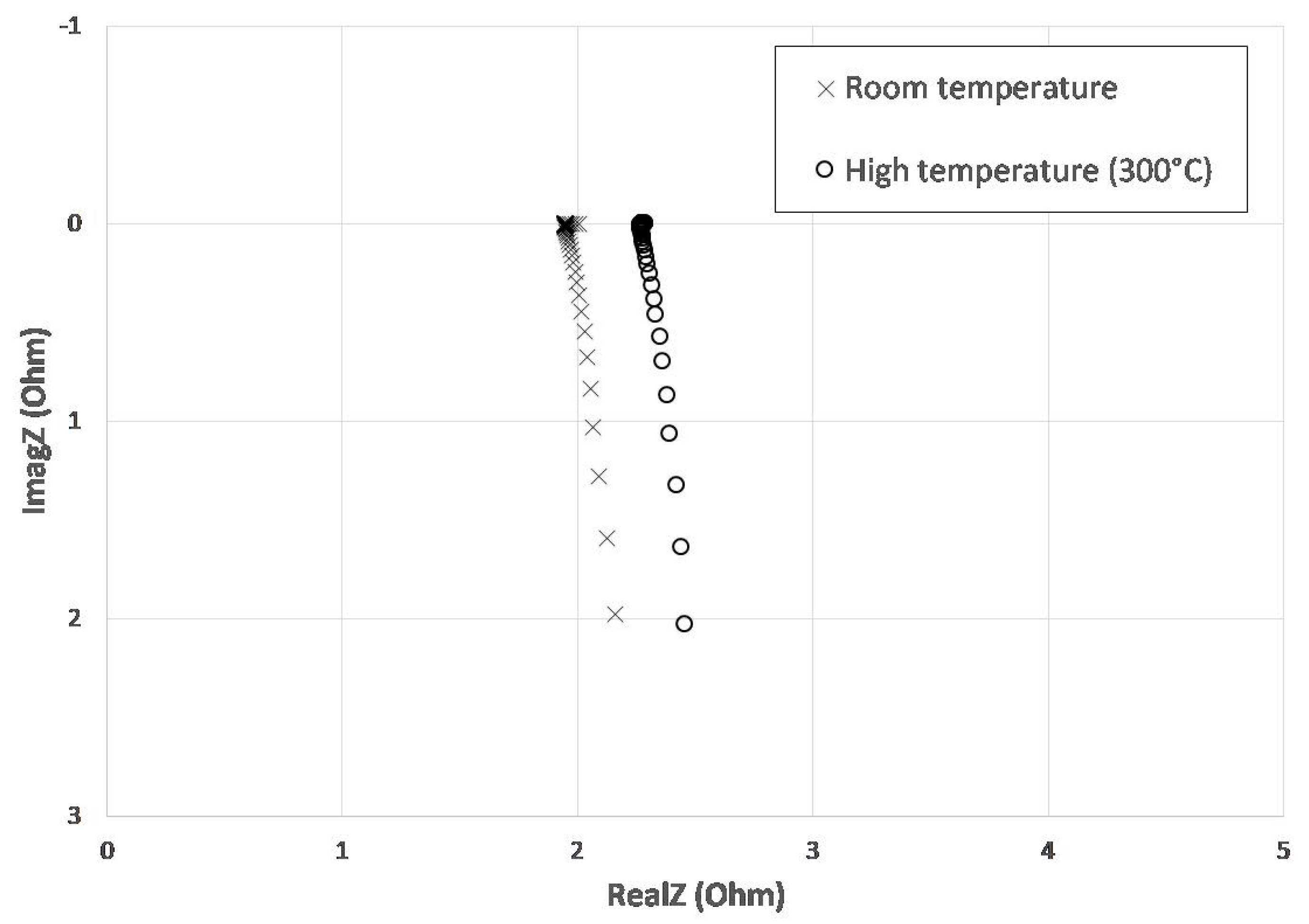
All impedance results show a high frequency arc. This high frequency arc can be a response of the system, but it can also be an artefact coming from the measuring device, i.e., the potentiostat and cell cable connections [25,26]. If the response is from the system, it can possibly be related to the oxide film that is formed during the high temperature exposure test. Another possibility is that it is related to the capacitance of the solution. This can happen when the system has a relatively high solution resistance. To be sure that we are not analyzing artefacts, but only real system responses, we have measured the impedance of the potentiostat and signal cables alone. This is done by connecting all the leads (WE, WE sense, RE, CE and CE sense) to each other. In this way the impedance of the potentiostat and leads are determined. Two measurements were carried out: the first one at room temperature in air, the second one in high temperature water at 300 °C.
The results of the two impedance tests are shown in Figure 7. Both the results at room temperature as well as the results at high temperature show inductive behavior and the spectrum fits well to a series RL model. Generally, this arises either from the inductance of the leads to the cell or from cell/potentiostat interactions [26]. From these results it is clear that the high frequency arc cannot be related to the measuring device or leads, but that it is a system response.
The high frequency arc observed in most of the Nyquist results of alloy 182 is most probably related to the oxide film capacitance and/or the space charge (diffuse double layer) capacitance. The latter is typical for systems with a relative high solution resistance. It can be a measurement of the capacitance of the solution, i.e., the space charge or diffuse double layer. The reason for this is that at low concentrations the cations and anions differ from their bulk concentrations. Ions of opposite charge cluster to the electrode surface, while ions of the same charge are repelled from it. Among others, this is described by the Gouy–Chapman model. The resulting differential capacitance depends strongly on the bulk concentration and the potential difference between the electrode and the solution [27,28].
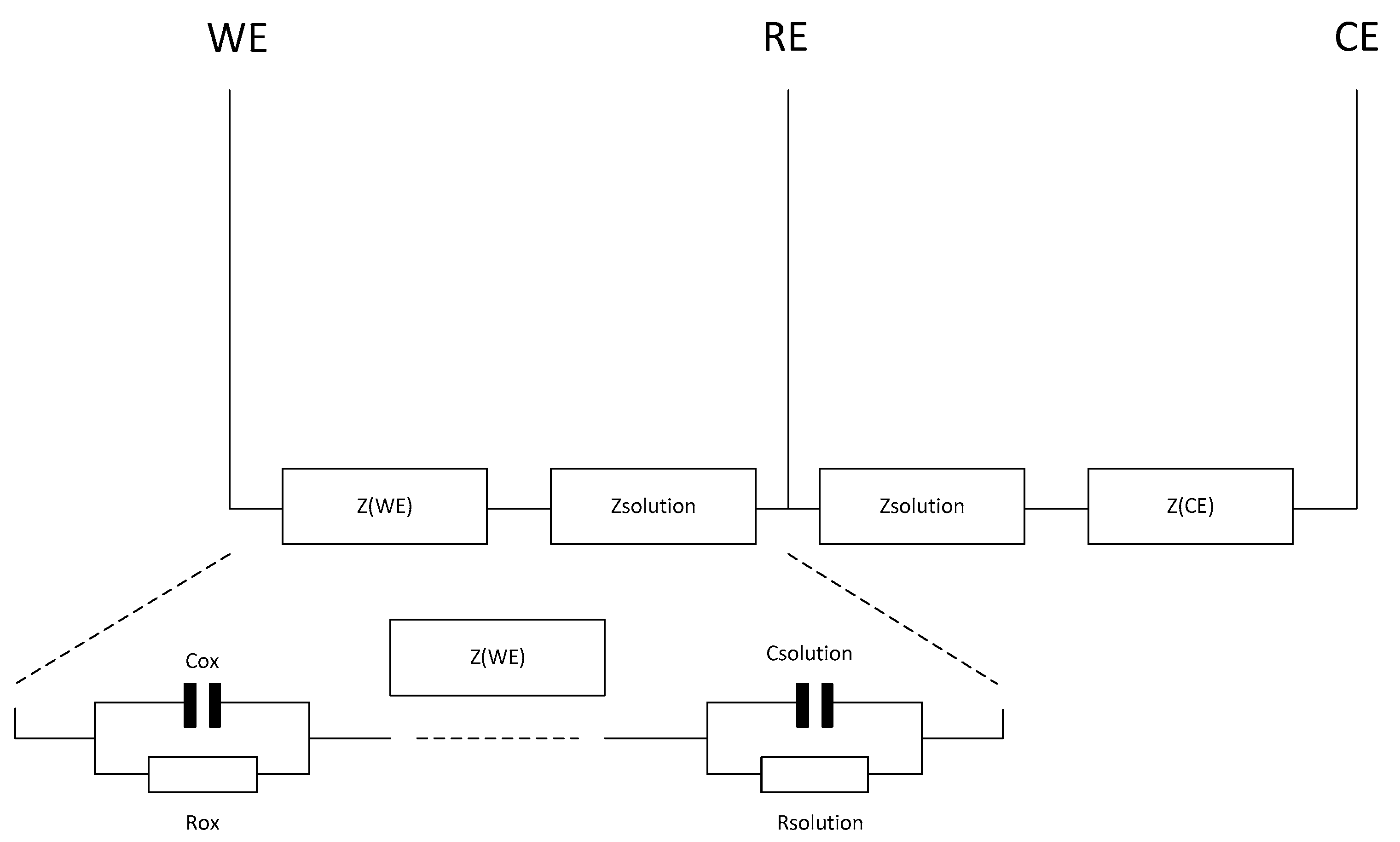
A simple calculation was carried out to see whether one can distinguish between the oxide film impedance and the solution impedance, both represented by a parallel circuit of a resistance and a capacitor as shown in Figure 8. A typical value for the space charge is 0.1 nF cm−2 [26]. A typical value for the oxide film capacity can be obtained with the following calculation:
where ε0 is the electric constant (F/m), εr is the dielectric constant of the oxide layer, A is the surface area of the electrode (m2) and d is the thickness of the oxide layer (m). Therefore, for the oxide capacitance a value of about 20.7 nF (or 10.7 nF/cm2) will be used. This is more than two orders of magnitude different from the space charge.
Besides the capacitance, also the ohmic resistance of the oxide film and diffuse double layer (≈solution resistance) differ. For the oxide layer resistance a value of 100 Ohm cm2 is used, based on Contact Electric Resistance (CER) measurement on Ni-Cr alloys [29]. The solution resistance is the difference between the ohmic resistance (Table 3) and the oxide layer resistance.
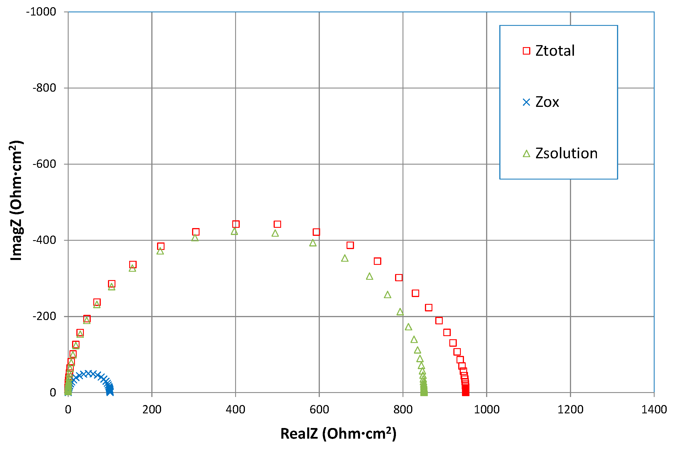
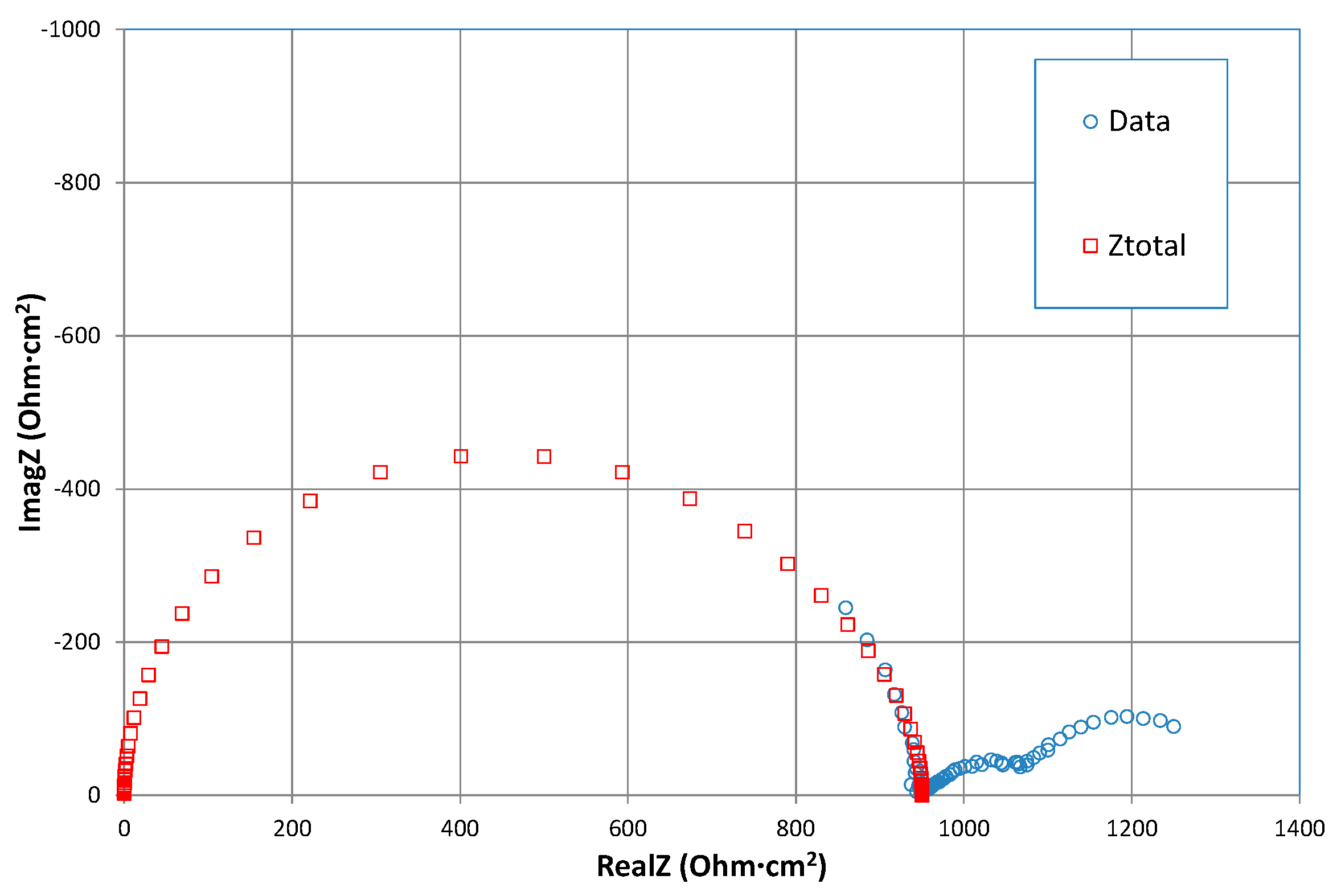
A simulation of the high frequency part of the impedance is plotted in Figure 9. The values in Table 4 were used to make the calculation. These values were taken from the fit results of Figure 10. The individual contributions of the oxide film and the solution are shown together with the total impedance. When using the values in Table 4, the impedance of the oxide film is hidden behind the impedance of the solution.
Depending on the exact values, the oxide film can still be visible or not. If we plot the simulation together with measured data, as shown in Figure 10, it is clear that the part of the oxide film impedance is barely visible. When longer exposure times are used, resulting in a thicker oxide film (with higher ohmic resistance), maybe a more pronounced result could be expected.
3.3. Interpretation of the Warburg Coefficient
The Warburg impedance is related to diffusion phenomena that are taking place at the electrode surface. It represents the electrochemical active species that are moving from and to the electrode surface. In this section the Warburg coefficient is calculated for the hydrogen oxidation reaction and compared with the experimentally obtained values. For a simple electrode reaction (Red ↔ Ox + e−) the Warburg coefficient σ is given by [23,24,28]:
in which R is the gas constant, T is the temperature, DO is the diffusion coefficient of the oxidant, DR is the diffusion coefficient of the reductant, A is the surface area of the electrode, n is the number of electrons involved, CO is the concentration of the oxidant and CR is the concentration of the reductant.
For corroding systems, the situation is far more complex, as the different electrochemical reactions where diffusion takes place will contribute to the Warburg impedance and as such to the Warburg coefficient. Here we will make a simple calculation to see whether indeed the hydrogen dominates the Warburg impedance. To do this we assume that the hydrogen oxidation is the main electrochemical reaction at the electrode surface. That is, it is assumed that this reaction is dominant with respect to the other reactions, like the oxidation of the surface leading to the oxide layers as shown in Figure 2. If the hydrogen oxidation (H2 ↔ 2H+ + 2e−) is the main contributor to the Warburg coefficient, Equation (5) changes to:
It is assumed that the backward reaction is not diffusion controlled due to the abandoned presence of the water. To calculate the Warburg coefficient for the four different test conditions the numbers shown in Table 5 were used. The hydrogen diffusion coefficients at high temperature were taken from reference [30]. Table 5 also shows a comparison between the measured Warburg coefficient and the calculated Warburg coefficient.
The calculated and measured Warburg coefficients for the Pt specimen are close together. As only redox reactions are considered here to take place, this makes sense. The morphologies of the Alloy 182 surfaces are quite different, as shown in Figure 2. For the specimens’ tests at 300 °C and 330 °C the surface is oxidized but is still relatively smooth. Therefore a Warburg impedance related to hydrogen diffusion should be a viable option. For 330 °C the calculated and measured Warburg coefficients for Alloy 182 specimen are relatively close, but at 300 °C this is much less the case. The calculated and measured Warburg coefficients for the 345 °C + 35 H2 cc/kg and the 330 °C + 5 H2 cc/kg test conditions are far away from each other. Looking at the surface morphologies of these specimens it is clear that the (simplified) equation for the Warburg coefficient does not cover all the diffusion phenomena that are taking place at the electrode surface. In conclusion, for the Pt and Alloy 182 at 330 °C the Warburg impedance is dominated by the hydrogen oxidation reaction. For the other test conditions, other phenomena can play a role and/or the Warburg impedance is not sufficient to describe the different processes that are taken place.
3.4. Trend Analysis of the Equivalent Circuit Fit Parameters
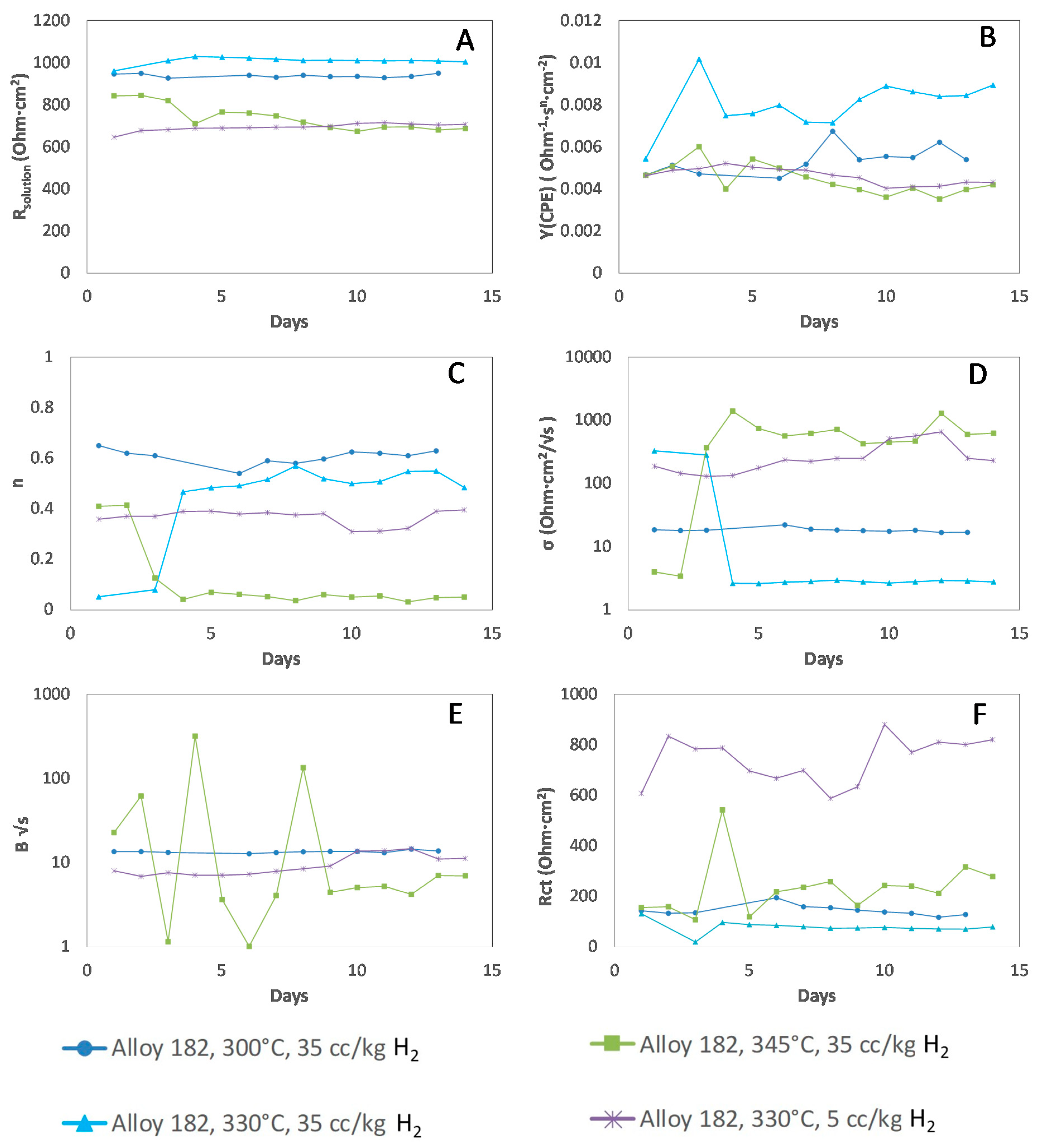
In this section the fit results of the equivalent circuit as shown in Figure 4 will be discussed. For each circuit element a plot was made where the value of interest is plotted as a function of time (two weeks) for each of the four tests. This allows one to see how these parameters develop over time and if their values can be used to distinguish between the different conditions and oxide layer morphologies.
Figure 11A shows the solution resistance (Rsolution) as a function of time. There is a difference between the four tests, but no evolution versus time. This is to be expected as the solution resistance is mainly affected by the water resistance, which should be more or less constant for each test condition.
Figure 11B shows the CPE constant related to the electrochemical double layer (Y) as a function of time. There is a difference between the four test runs and also a small change in time. The CPE constant reflects the value of the electrochemical double layer, which can change over time due to the changes in oxide morphologies of the specimen surface which then changes the effective surface area. This is more pronounced for the conditions where there are needles (345 °C, 35 cc/kg H2) or crystallites (330 °C, 5 cc/kg H2) on the surface.
Figure 11C shows the CPE coefficient (n) as a function of time. This n value can be related to the surface roughness or tortuosity of the oxide layer. The lower the number, the higher the deviation from a smooth surface. The n values clearly reflect the surface morphologies as shown in Figure 1. For the relatively smooth surfaces (300 °C, 35 cc/kg H2 and 330 °C, 35 cc/kg H2) the value is the highest. For the rough and irregular surfaces (330 °C, 5 cc/kg H2 and 345 °C, 35 cc/kg H2) the values are the lowest.
Figure 11D shows the Warburg coefficients as functions of time. Y(cotanh) is the coefficient of the finite Warburg impedance and W is the coefficient of the infinite Warburg impedance. It can be noticed that there is a quite large difference between the four test conditions. A lower hydrogen concentration means a higher Warburg impedance and so a smaller coefficient; therefore the result for the 5 cc/kg H2 makes sense. For the 35 cc/kg H2 one would expect some influence of the temperature and as such 330 °C has a higher coefficient than 300 °C. The 345 °C is not consistent with the other two, but the surface is highly irregular (needle like oxides). That means that the diffusion processes are seriously hampered, resulting in a smaller coefficient.
Figure 11E shows the values of the Warburg fit parameter B (represented by δ/√D). The B parameter is a measure for the length of the diffusion layer thickness. With increasing size of this B parameter, the finite Warburg changes to an infinite Warburg impedance. There is a large scatter for 345 °C (again related to the highly dispersed surface of the specimen under this test condition), and the values are around ten. For the W fit of 330 °C there is no plot of the B parameter as it is close to infinite (B→∞).
Figure 11F shows the charge transfer resistance as a function of time for the four different test conditions. These results are in good agreement with the observed surface conditions and the water chemistry. The higher the temperature, the higher the reaction kinetics and so the lower the resistance. The 345 °C results are as expected to be above the 300 °C results. The low hydrogen concentration (5 cc/kg H2) is much higher than the 35 cc/kg H2. The 345 °C results are a bit in between, which is due to the highly dispersed surface area.
Concluding remarks: The results of the fit parameters obtained with the equivalent circuit analysis are consistent with respect to the test temperature, hydrogen concentration and surface conditions. The CPE exponent (n) and charge transfer resistance (Rct) show the most pronounced differences between the different test conditions. Here the CPE exponent (n) can be associated with the surface morphology. A high surface roughness or high degree of tortuosity results in a larger dispersion of the electrochemical processes and so a smaller value of n. The charge transfer resistance (Rct) is typically related to the water chemistry. More hydrogen and higher temperatures result in faster kinetics and as such a smaller value of Rct. These correlations do not necessarily have a one to one relationship with the SCC susceptibility. Therefore, in the Discussion section the “Crack growth rate factor” is introduced, which will be used to make a quantitative correlation between the impedance results and the SCC susceptibility.
3.5. Low Frequency Impedance Analysis
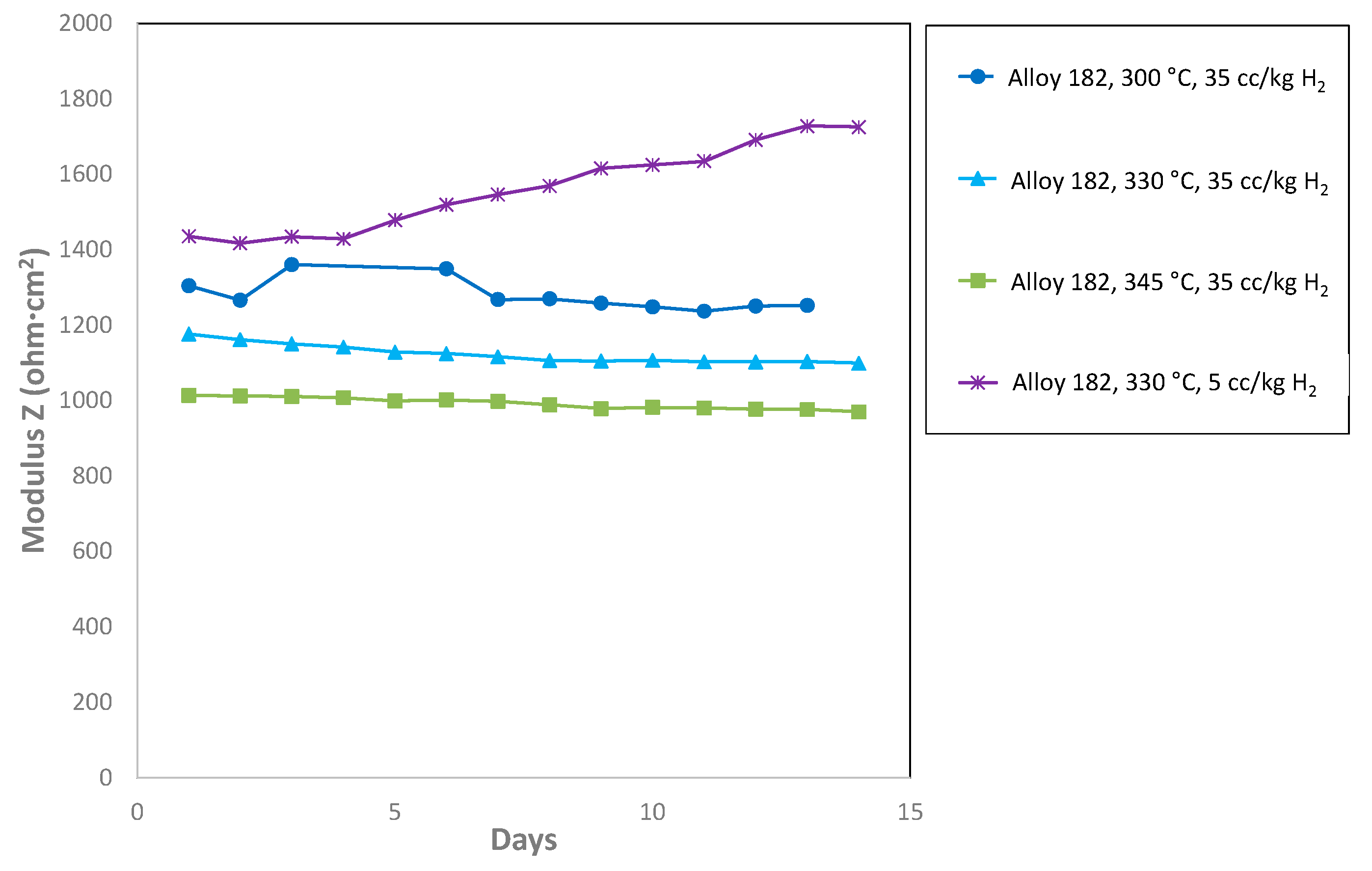
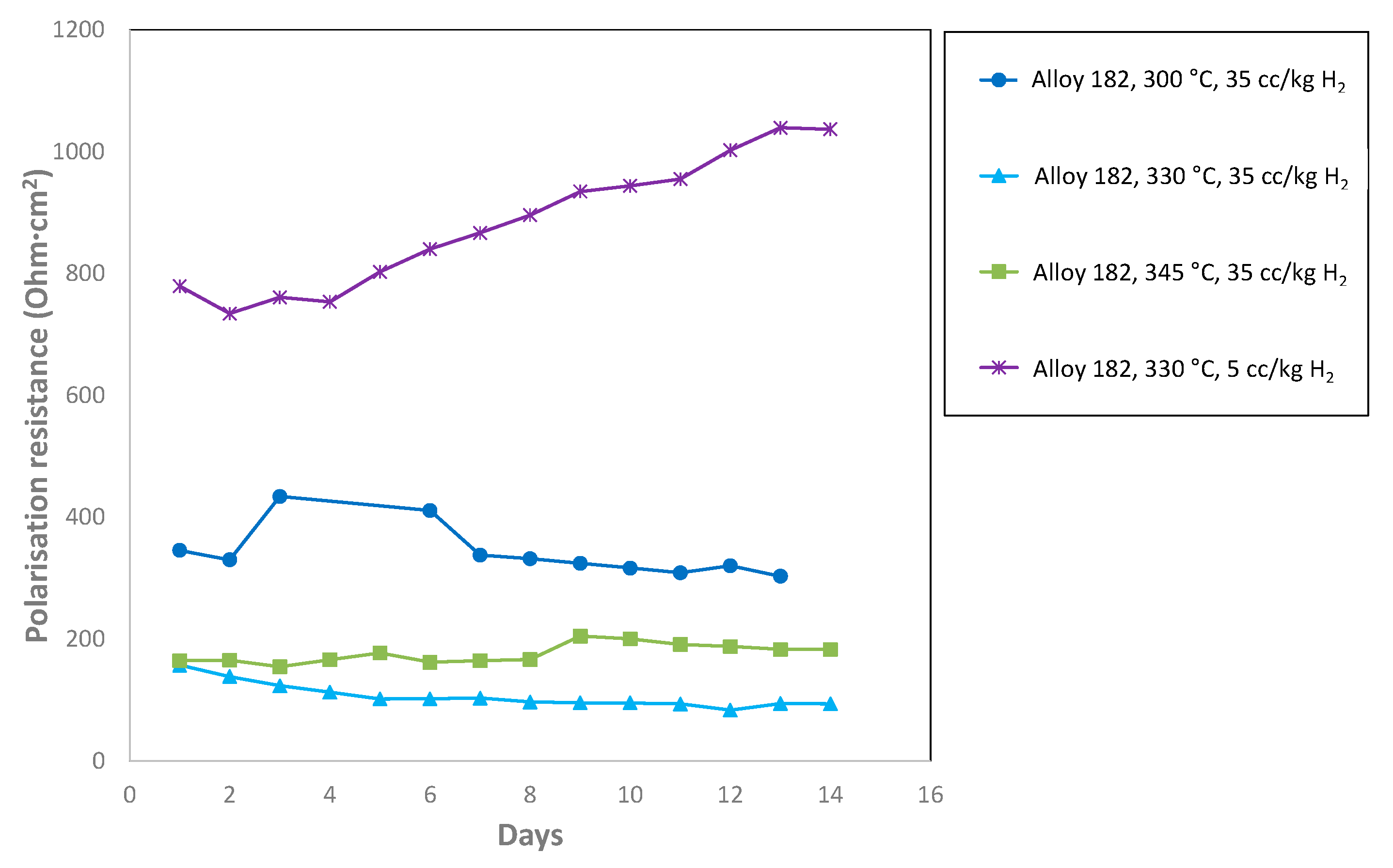
In this section the impedance data is interpreted without using an equivalent circuit model. Values of the impedance were directly taken from the impedance diagrams and plotted as a function of time for the four different test conditions. Figure 12 shows the modulus of the low frequency impedance, which is the impedance at 1 mHz. Figure 13 shows the polarization resistance obtained from the impedance diagram, which is the difference between the low frequency impedance and the solution resistance.
Figure 12 shows a clear and distinct difference between the four test conditions. The highest impedance is measured at the lowest hydrogen concentration. This makes sense as hydrogen is a dominant factor in the impedance and less hydrogen means a higher impedance. It can also be noticed that the impedance is decreasing with increasing temperature. This makes sense as well, as the reaction kinetics do increase with temperature, resulting in a lower impedance.
Figure 13 shows that the polarization resistance follows more or less the same trend as the low frequency impedance in Figure 12. The polarization resistance is solely related to the electrochemical processes at the interface, while the low frequency impedance is also influenced by the solution resistance. The only difference here is that the results of the two highest temperatures are switched. This might be due to the fact that the surface conditions are different.
4. Discussion
The main aim of this work is to find a correlation between the in-situ impedance measurements and the SCC susceptibility of Alloy 182 at the different test conditions. The overall impedance response reflects quite well the water chemistry (temperature and hydrogen concentration) as shown in Figure 12. However this doesn’t necessarily reflect the degree of SCC susceptibility. Also the dots in Figure 1 represent only a semi-quantitative measure for the SCC susceptibility, being the distance to the Ni/NiO transition line.
A more quantitative estimate of the SCC susceptibility can be made using a model proposed by Attanasio and Morton [4,20], which was further developed by Andresen [3,31]. This model is based on trend curve analysis of a large number of SCC crack growth rate tests with Ni-based Alloys at different concentrations of dissolved hydrogen. With this model the peak in SCC crack growth rate can be calculated as function of temperature and hydrogen concentration. It can also be used to calculate the relative crack growth rate as a function of hydrogen concentration and temperature. This allows us to determine for each of the test conditions (as mentioned in Section 2) a value for the crack growth rate factor. This crack growth rate factor is the difference between the lowest and highest crack growth rate around the Ni/NiO transition line. A short summary of this model is given here, taken from the EPRI MRP-115 report [31].
This crack growth rate factor is defined as
where Vp is the crack growth rate velocity relative to the peak height, P is the height of the peak, λ is the width of the peak, ECPos is the offset of the CGR peak from the Ni/NiO phase boundary and ∆ECP is the H2 value versus peak H2.
The ∆ECP is given by
In Equation (8) the hydrogen concentration that corresponds with the Ni/NiO transition as a function of temperature is given by:
With these three equations the crack growth rate velocity to the peak height can be calculated. It is assumed that this ratio to the peak height is similar at different temperatures, but not the crack growth rate itself. Therefore, the temperature dependence must be calculated, using the following equation.
where VR is the ratio of the crack growth rate at one temperature (T2) versus another temperature (T1), Q is the activation enthalpy, R is the molar gas constant and T is the temperature in K. The necessary parameters are summarized in Table 6.
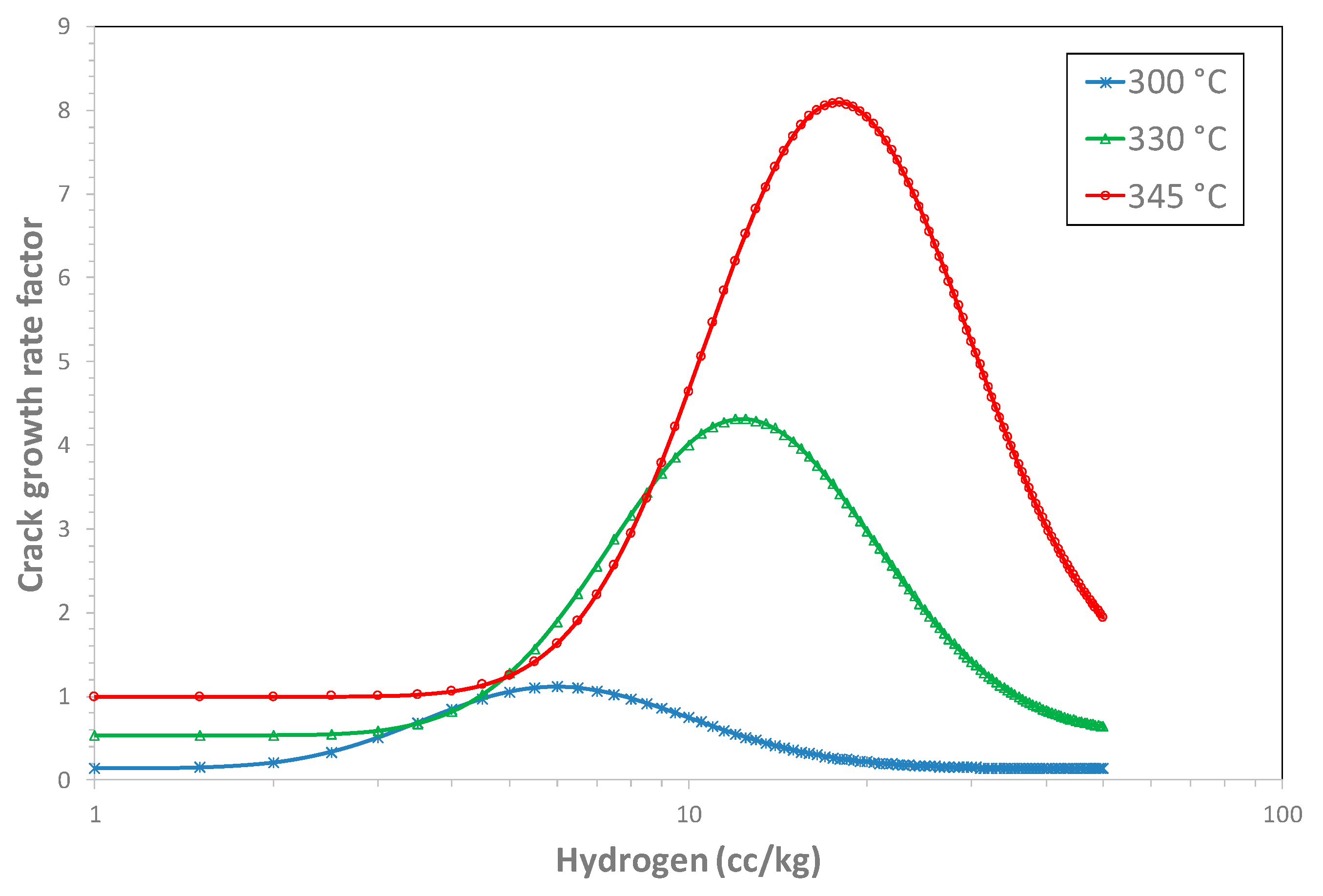
The above mentioned equations were used to calculate the crack growth rate factors as a function of hydrogen concentration for the three test temperatures (300, 330 and 345 °C) used in this work. Figure 14 shows the results. It is clear that the higher the temperature, the higher the peak, which in its turn is shifting to the right at regions of higher hydrogen concentrations.
From these results a crack growth rate factor for each test condition can be determined as shown in Table 7.
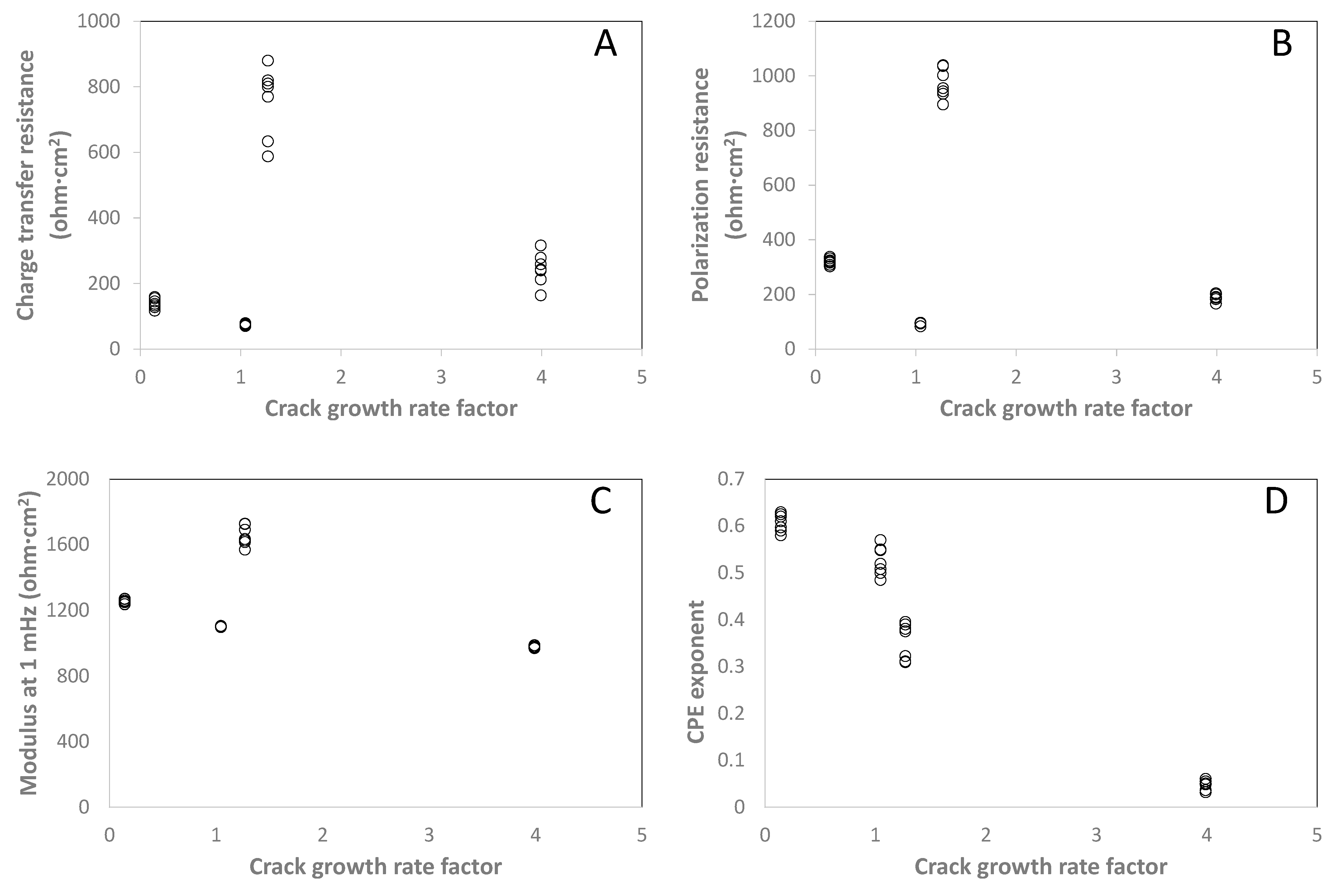
Figure 15 shows the impedance parameters (Rct, Rp, Rz and n) as functions of the crack growth rate factor. The impedance parameters of the last seven measurements (day 8 to day 14) were plotted, assuming that more or less stable conditions were reached after one week of testing. The parameter that shows the best correlation with the crack growth rate factor is the CPE exponent n (Figure 15D). This exponent can be seen as a representative of the surface roughness or tortuosity of the surface oxides. The lower this value the more irregular the surface and/or the larger the dispersion at the surface. It shows the best correlation with the SCC susceptibility of all the circuit parameters, where a low value is related to a higher SCC susceptibility and vice versa.
5. Conclusions
In-situ EIS measurements were carried out in high temperature water with Ni-based Alloy 182, with the main aim to correlate the EIS results with the differences in stress corrosion cracking (SCC) susceptibility that is present around the Ni-NiO transition.
During the measurement time of two weeks little or no evolution of the impedance was observed, which meant that the impedance was dominated by the water chemistry (dissolved hydrogen). This was confirmed by the measurement on platinum, which had a similarly shaped impedance response (although different in magnitude), as the Ni Alloys.
First, a simple equivalent circuit model was used to interpret the EIS data. It was shown that the CPE exponent n, which is a measure of the degree of roughness or dispersion of the surface area, could be correlated to the different test conditions. The lowest value for n was obtained for the test condition 345 °C and 35 cc/kg H2, which had the most dispersed surface morphology. A comparison with the SCC susceptibility, expressed in a crack growth rate factor after a model of Morton/Andresen, showed the same correlation.
Second, the low frequency impedance values measured at 1 mHz allowed to make a clear distinction between the four test conditions. The highest impedance was at the lowest hydrogen concentration whereas the lowest impedance was at the highest temperature and hydrogen concentration.
In addition, it was shown that the high frequency arc, commonly present at EIS data in high temperature water, was related to the diffuse double layer present at the hot water/metal interface.
Author Contributions
Conceptualization, R.-W.B. and M.V.; methodology, R.-W.B. and M.V.; formal analysis, R.-W.B.; investigation, R.-W.B.; writing—original draft preparation, R.-W.B.; writing—review and editing, M.V.; visualization, R.-W.B. Both authors have read and agreed to the published version of the manuscript.
Funding
This research received no external funding.
Institutional Review Board Statement
Not applicable.
Informed Consent Statement
Not applicable.
Data Availability Statement
The data presented in this study are available in this article.
Conflicts of Interest
The authors declare no conflict of interest.
References
- Scott, P.M.; Combrade, P. Corrosion in Pressurized Water Reactors. In ASM Handbook, Volume 13C Corrosion: Environments and Industries; ASM International: Materials Park, OH, USA, 2006; ISBN 13: 978-0-87170-709-3. [Google Scholar]
- Vaillant, F.; Boursier, J.-M.; Amzallag, C.; Bibollet, C.; Pons, S. Environmental Behaviour and weldability of Ni-base weld in PWRs. Rev. Générale Nucléaire 2007, 6, 62–71. [Google Scholar] [CrossRef]
- Andresen, P.L.; Hickling, J.; Ahluwalia, A.; Wilson, J. Effects of Hydrogen on SCC Growth Rate of nickel Alloys in high temperature water. Corrosion 2008, 64, 707–720. [Google Scholar] [CrossRef]
- Attanasio, S.A.; Morton, D.S. Measurement of the Nickel Oxide Transition in Ni-Cr-Fe Alloys and Updated Data and Correlations to Quantify the Effect of Aqueous Hydrogen on Primary Water SCC. In Proceedings of the 11th International Conference Environmental Degradation of Materials in Nuclear Power Systems, Stevenson, WA, USA, 10–14 August 2003. [Google Scholar]
- Liu, J.-H.; Mendonça, R.; Bosch, R.-W.; Konstantinović, M.J. Characterization of oxide films formed on alloy 182 in simulated PWR primary water. J. Nucl. Mater. 2009, 393, 242–248. [Google Scholar] [CrossRef]
- Terachi, T.; Totsuka, N.; Yamada, T.; Nakagawa, T.; Deguchi, H.; Masaki, H.; Oshitani, M. Influence of dissolved hydrogen on structure of oxide film on alloy 600 formed in primary water of pressurized water reactors. J. Nucl. Sci. Technol. 2003, 40, 509–516. [Google Scholar] [CrossRef]
- Kuang, W.; Wu, X.; Han, E.-H. Influence of dissolved oxygen concentration on the oxide film formed on Alloy 690 in high temperature water. Corros. Sci. 2013, 69, 197–204. [Google Scholar] [CrossRef]
- Dozaki, K.; Akutagawa, D.; Nagata, N.; Takiguchi, H.; Norring, K. Effects of dissolved hydrogen content in PWR primary water on PWSCC initiation property. E-J. Adv. Maint. Jpn. Soc. Maintenology 2010, 2, 65–76. [Google Scholar]
- Mendonça, R.; Bosch, R.W.; van Renterghem, W.; Vankeerberghen, M.; Figueiredo, C.d. Effect of temperature and dissolved hydrogen on oxide films formed on Ni and Alloy 182 in simulated PWR water. J. Nucl. Mater. 2016, 477, 280–291. [Google Scholar] [CrossRef]
- Figueiredo, C.; Bosch, R.-W.; Vankeerberghen, M. Electrochemical investigation of oxide films formed on nickel alloys 182, 600 and 52 in high temperature water. Electrochim. Acta 2011, 56, 7871–7879. [Google Scholar] [CrossRef]
- Bosch, R.W.; Vankeerberghen, M. In-pile electrochemical tests of stainless steel under PWR conditions: Interpretation of electrochemical impedance spectroscopy data. Electrochim. Acta 2007, 52, 7538. [Google Scholar] [CrossRef]
- Xu, J.; Shoji, T. The corrosion behavior of Alloy 182 in a cyclic hydrogenated and oxygenated water chemistry in high temperature aqueous environment. Corros. Sci. 2016, 104, 248. [Google Scholar] [CrossRef]
- Wang, J.; Wang, J.; Ming, H.; Zhang, Z.; Han, E.H. Effect of temperature on corrosion behavior of alloy 690 in high temperature hydrogenated water. J. Mater. Sci. Technol. 2018, 34, 1419. [Google Scholar] [CrossRef]
- Yang, J.; Li, Y.; Xu, A.; Fekete, B.; Macdonald, D.D. The electrochemical properties of alloy 690 in simulated pressurized water reactor primary water: Effect of temperature. J. Nucl. Mater. 2019, 518, 305. [Google Scholar] [CrossRef]
- Yang, J.; Li, Y.; Macdonald, D.D. Effects of temperature and pH on the electrochemical behaviour of alloy 600 in simulated pressurized water reactor primary water. J. Nucl. Mater. 2020, 528, 151850. [Google Scholar] [CrossRef]
- Xu, J.; Shoji, T.; Jang, C. The effects of dissolved hydrogen on the corrosion behavior of Alloy 182 in simulated primary water. Corros. Sci. 2015, 97, 115. [Google Scholar] [CrossRef]
- Bai, J.; Bosch, R.W.; Ritter, S.; Schneider, C.; Seifert, H.P.; Virtanen, S. Electrochemical and spectroscopic characterization of oxide films formed on Alloy 182 in simulated boiling water reactor environments: Effects of dissolved hydrogen. Corros. Sci. 2018, 133, 204. [Google Scholar] [CrossRef]
- Macak, J.; Sajdl, P.; Kucera, P.; Novotny, R.; Vosta, J. In situ electrochemical impedance and noise measurements of corroding stainless steel in high temperature water. Electrochim. Acta 2006, 51, 3566. [Google Scholar] [CrossRef]
- Macak, J.; Novotny, R.; Sajdl, P.; Bystriansky, V.; Tuma, L.; Novak, M. In-situ electrochemical impedance measurements of corrosing stainless steel in high subcritical water. Corros. Sci. 2019, 150, 9. [Google Scholar] [CrossRef]
- Morton, D.S.; Attanasio, S.A.; Richey, E.; Young, G.A. In search of the true temperature and stress intensity factor dependencies for PWSCC. In Proceedings of the 12th International Conference Environmental Degradation of Materials in Nuclear Power Systems, TMS (The Minerals, Metals & Materials Society), Salt Lake, UT, USA, 14–18 August 2005. [Google Scholar]
- PWR Primary Water Chemistry Guidelines: Volume 1, Revision 4; EPRI: Palo Alto, CA, USA, 1999.
- Wood, C.J. 5.02 Water Chemistry control in LWRs. Compr. Nucl. Mater. 2012, 5, 17. [Google Scholar]
- Basics of Electrochemical Impedance Spectroscopy. In Application Note Gamry Instruments; Gamry Instruments: Warminster, PA, USA, 2006.
- Cottis, R.A.; Turgoose, S.; Neuman, R. Electrochemical Impedance and Noise. In Corrosion Testing Made Easy; NACE International: Houston, TX, USA, 1999. [Google Scholar]
- Stewart, K.C.; Kolman, D.G.; Taylor, S.R. The effect of parasitic conduction pathways on EIS measurements in low conductivity media. In Electrochemical Impedance: Analysis and Interpretation; Scully, J., Silverman, D., Kendig, M., Eds.; ASTM STP1188: West Conshohocken, PA, USA, 1993. [Google Scholar]
- Quick check of EIS System Performance. In Appliction Note Gamry Instruments; Gamry Instruments: Warminster, PA, USA, 2013.
- Bockris, J.O.M.; Reddy, A.K.N. Modern Electrochemistry; Plenum Press: New York, NY, USA, 1970. [Google Scholar]
- Bard, A.J.; Faulkner, L.R. Electrochemical Methods; Wiley & Sons: Hoboken, NJ, USA, 1980. [Google Scholar]
- Bojinov, M.; Kinnunen, P.; Sundholm, G. Electrochemical behavior of Nickel-Chromium Alloys in a high-temperature aqueous electrolyte. Corrosion 2003, 59, 91. [Google Scholar] [CrossRef]
- Kalligras, D.T.; Plugatry, A.Y.; Svishchev, I.M. High temperature diffusion coefficients for O2, H2 and OH in water, and for pure water. J. Chem. Eng. Data 2014, 59, 1964. [Google Scholar] [CrossRef]
- Materials Reliability Program: Mitigation of PWSCC in Nickel-Base Alloys by Optimizing Hydrogen in the Primary Water (MRP-213); EPRI: Palo Alto, CA, USA, 2007; p. 1015288.
Figure 1.
The nickel–nickel oxide transition curve as a function of temperature and dissolved hydrogen concentration showing the selected test conditions for the EIS measurements and related surface morphology. Solid line data from Andresen [3]; dashed line data from Terachi [6].

Figure 2.
Dissimilar metal weld of Alloy 182 between SA-508 (left) and 316 L (right).

Figure 3.
(A) Electrode arrangement in the autoclave Pt reference electrode (RE), Alloy 182 working electrode (WE) and autoclave body as counter electrode (CE), (B) mineral insulated signal cable with special ceramic connector, (C) Alloy 182 specimen connected to the cable and ceramic connector.
Figure 3.
(A) Electrode arrangement in the autoclave Pt reference electrode (RE), Alloy 182 working electrode (WE) and autoclave body as counter electrode (CE), (B) mineral insulated signal cable with special ceramic connector, (C) Alloy 182 specimen connected to the cable and ceramic connector.

Figure 4.
Equivalent circuit model for the metal-oxide-solution interface of Alloy 182 in high temperature water containing an oxide layer capacity (Cox), an oxide resistance (Rox), a charge transfer resistance (Rct), a diffusion resistance for finite length diffusion layer (O) or a diffusion resistance for infinite length diffusion layer (W), a Constant Phase Element (CPE), a solution capacitance (Csolution) and a solution resistance (Rsolution).

Figure 5.
EIS results after eight days of testing at 300 °C and 35 cc/kg dissolved hydrogen. Red circles = measured data, Blue crosses = fit result.
Figure 5.
EIS results after eight days of testing at 300 °C and 35 cc/kg dissolved hydrogen. Red circles = measured data, Blue crosses = fit result.

Figure 6.
Nyquist diagrams after eight days of testing.

Figure 7.
EIS results of the leads and potentiostat (Nyquist plot).

Figure 8.
High frequency impedance is related to the oxide layer impedance and solution impedance (=solution resistance + solution capacitance).
Figure 8.
High frequency impedance is related to the oxide layer impedance and solution impedance (=solution resistance + solution capacitance).

Figure 9.
High frequency part of the impedance: oxide layer (blue cross), solution (green dash) and total high frequency impedance (red square).
Figure 9.
High frequency part of the impedance: oxide layer (blue cross), solution (green dash) and total high frequency impedance (red square).

Figure 10.
Fit of the high frequency part of the impedance with the impedance model containing only the oxide layer and solution impedance (ohmic resistance and space charge).
Figure 10.
Fit of the high frequency part of the impedance with the impedance model containing only the oxide layer and solution impedance (ohmic resistance and space charge).

Figure 11.
Fit results as a function of time: (A) solution resistance Rsolution, (B) CPE constant Y(CPE), (C) CPE exponent n, (D) Warburg coefficient σ, (E) diffusion parameter B, and (F) charge transfer resistance Rct.
Figure 11.
Fit results as a function of time: (A) solution resistance Rsolution, (B) CPE constant Y(CPE), (C) CPE exponent n, (D) Warburg coefficient σ, (E) diffusion parameter B, and (F) charge transfer resistance Rct.

Figure 12.
Modulus of the impedance at low frequency as a function of time.

Figure 13.
Polarisation resistance as a function of time determined as the difference between the low impedance and the high frequency intersect with the real axis, as a function of time.
Figure 13.
Polarisation resistance as a function of time determined as the difference between the low impedance and the high frequency intersect with the real axis, as a function of time.

Figure 14.
Calculated effect of hydrogen on the crack growth rate factor of Nickel-Base Alloys for the temperatures 300 °C, 330 °C and 345 °C.
Figure 14.
Calculated effect of hydrogen on the crack growth rate factor of Nickel-Base Alloys for the temperatures 300 °C, 330 °C and 345 °C.

Figure 15.
Impedance fit parameters (Rct, Rp, Rz and n) as a function of crack growth rate factor: (A) Charge transfer resistance Rct, (B) Polarization resistance Rp, (C) low frequency modulus RZ, (D) CPE exponent n.
Figure 15.
Impedance fit parameters (Rct, Rp, Rz and n) as a function of crack growth rate factor: (A) Charge transfer resistance Rct, (B) Polarization resistance Rp, (C) low frequency modulus RZ, (D) CPE exponent n.


Table 1.
Chemical composition of the Alloy 182 weld metal.
| Alloy | C | Cr | Fe | Ni | Mn | Si | P | S | Nb | Ti | Cu | Mo |
|---|---|---|---|---|---|---|---|---|---|---|---|---|
| 182 | 0.047 | 14.9 | Bal. | 71.8 | 5.81 | 0.015 | 0.015 | 0.006 | 1.89 | 0.183 | 0.019 | 0.24 |
Table 2.
Test matrix of the impedance measurements.
| Test nr | Working Electrode | Temperature | Hydrogen Concentration |
|---|---|---|---|
| 1 | Alloy 182 | 300 °C | 35 cc/kg H2 |
| 2 | Alloy 182 | 330 °C | 35 cc/kg H2 |
| 3 | Alloy 182 | 345 °C | 35 cc/kg H2 |
| 4 | Alloy 182 | 330 °C | 5 cc/kg H2 |
| 5 | Pt | 330 °C | 35 cc/kg H2 |
Table 3.
Fit results of the equivalent circuit model after eight days of testing.
| Test Condition | Material | Rsolution (Ohm·cm2) | Yo (Ohm−1·sn·cm−2) | n | σ (Ohm·s−½·cm2) | B | Rct (Ohm·cm2) |
|---|---|---|---|---|---|---|---|
| 300 °C, 35 cc/kg H2 | Alloy 182 | 940 | 6.74 × 10⁻³ | 0.580 | 18.36 | 13.5 | 155 |
| 330 °C, 35 cc/kg H2 | Alloy 182 | 1009 | 7.15 × 10⁻³ | 0.519 | 2.96 | -- | 74 |
| 345 °C, 35 cc/kg H2 | Alloy 182 | 717 | 4.22 × 10⁻³ | 0.037 | 719 | 134.0 | 259 |
| 330 °C, 5 cc/kg H2 | Alloy 182 | 694 | 4.65 × 10⁻³ | 0.376 | 249 | 8.5 | 588 |
| 330 °C, 35 cc/kg H2 | Pt | 652 | 1.48 × 10⁻³ | 0.459 | 6.88 | 23.8 | 103 |
Table 4.
Values for the high frequency impedance calculation.
| Oxide Layer Impedance | |
| Rox | 100 Ohm cm2 |
| Cox | 10.7 nF/cm2 |
| Solution Resistance and Capacitance (“Space Charge” or Diffuse Double Layer) | |
| Rsolution | 850 Ohm cm2 |
| Csolution | 0.1 nF/cm2 |
Table 5.
Comparison of the calculated and measured Warburg coefficients.
| Test Condition | Material | Temperature (K) | Hydrogen Concentration (mol/cm3) | Hydrogen Diffusion Coefficient (cm2/s) | σ Calculated (Ohm·s−½·cm2) | σ Measured (Ohm·s−½·cm2) |
|---|---|---|---|---|---|---|
| 300 °C, 35 cc/kg H2 | Alloy 182 | 573 | 1.56 × 10⁻⁶ | 4.81 × 10⁻⁴ | 3.71 | 18.36 |
| 330 °C, 35 cc/kg H2 | Alloy 182 | 603 | 1.56 × 10⁻⁶ | 5.64 × 10⁻⁴ | 4.02 | 2.96 |
| 345 °C, 35 cc/kg H2 | Alloy 182 | 618 | 1.56 × 10⁻⁶ | 6.12 × 10⁻⁴ | 4.22 | 719 |
| 330 °C, 5 cc/kg H2 | Alloy 182 | 603 | 2.23 × 10⁻⁷ | 5.64 × 10⁻⁴ | 28.12 | 249 |
| 330 °C, 35 cc/kg H2 | Pt | 603 | 1.56 × 10⁻⁶ | 5.64 × 10⁻⁴ | 4.02 | 6.88 |
Table 6.
Values of the parameters used to calculate the crack growth rate factor [31].
Table 6.
Values of the parameters used to calculate the crack growth rate factor [31].
| Description | Value |
|---|---|
| H2(peak) at 300 °C | 5.50 cc/kg |
| H2(peak) at 330 °C | 11.83 cc/kg |
| H2(peak) at 345 °C | 17.34 cc/kg |
| P | 8.09 |
| ECPos | 0 |
| λ | 20.2 mV |
| Q | 130 kJ/mol |
| R | 8.314 J/mol-K |
Table 7.
Crack growth rate factor for each test condition.
| 300 °C, 35 cc/kg H2 | 330 °C, 35 cc/kg H2 | 345 °C, 35 cc/kg H2 | 330 °C, 5 cc/kg H2 | |
|---|---|---|---|---|
| CGR factor | 0.142 | 1.045 | 3.99 | 1.27 |
Publisher’s Note: MDPI stays neutral with regard to jurisdictional claims in published maps and institutional affiliations. |
© 2021 by the authors. Licensee MDPI, Basel, Switzerland. This article is an open access article distributed under the terms and conditions of the Creative Commons Attribution (CC BY) license (https://creativecommons.org/licenses/by/4.0/).
Share and Cite
MDPI and ACS Style
Bosch, R.-W.; Vankeerberghen, M. Differentiation of SCC Susceptibility with EIS of Alloy 182 in High Temperature Water. Corros. Mater. Degrad. 2021, 2, 341-359. https://0-doi-org.brum.beds.ac.uk/10.3390/cmd2030018
AMA Style
Bosch R-W, Vankeerberghen M. Differentiation of SCC Susceptibility with EIS of Alloy 182 in High Temperature Water. Corrosion and Materials Degradation. 2021; 2(3):341-359. https://0-doi-org.brum.beds.ac.uk/10.3390/cmd2030018
Chicago/Turabian StyleBosch, Rik-Wouter, and Marc Vankeerberghen. 2021. "Differentiation of SCC Susceptibility with EIS of Alloy 182 in High Temperature Water" Corrosion and Materials Degradation 2, no. 3: 341-359. https://0-doi-org.brum.beds.ac.uk/10.3390/cmd2030018