Validation of the Lattice Boltzmann Method for Simulation of Aerodynamics and Aeroacoustics in a Centrifugal Fan


Institute of Fluid Mechanics and Fluid Machinery, University of Kaiserslautern, Gottlieb-Daimler-Str. 44, 67663 Kaiserslautern, Germany
*
Author to whom correspondence should be addressed.
Acoustics 2020, 2(4), 735-752; https://0-doi-org.brum.beds.ac.uk/10.3390/acoustics2040040
Submission received: 1 September 2020
/
Revised: 18 September 2020
/
Accepted: 21 September 2020
/
Published: 26 September 2020
(This article belongs to the Special Issue Aeroacoustics of Turbomachines)
Abstract
:Due to the fact that legal and market requirements are becoming stricter, fan noise reduction, in addition to energy efficiency, represent a challenge for fan product designers. Most experimental studies are associated with trial-and-error approaches. Therefore, numerical methods are mostly preferable. However, the quantitative prediction of the noise emitted by radial fans via numerical simulations remains challenging. The Lattice Boltzmann method (LBM) is a relatively new approach that promises a direct calculation of the aerodynamics coupled with the aeroacoustics. This article presents an LBM simulation of a centrifugal fan using the commercial Lattice Boltzmann Code SIMULIA PowerFLOW of Dassault Systèmes. The simulation model includes both the fan impeller and the spiral housing. In accordance with the experimental setup, the fan was mounted in a test bench to analyze four different operating points. The results of the LBM simulation were validated by experimental measurements. Flow information in terms of pressure rise and efficiency of the centrifugal fan as a function of the flow rate are in a good agreement. Considering the acoustic spectra and the blade passing frequency, the simulation was able to precisely predict the noise of the centrifugal fan. The simulation results are also used to visualize the flow and acoustic field inside of the fan to detect noise-generating flow features. By evaluating the filtered pressure fluctuation in the fluid volume and on the wall, four main noise sources of the centrifugal fan can be identified.
1. Introduction
Noise generated by fans—whether they are broadband or tonal noises—can affect work place conditions of operators and often lead to annoyance for people in their vicinity. Legal and market requirements are also becoming stricter. Therefore, fan noise reduction in addition to energy efficiency represent a challenge for product designers.
Here, most experimental studies are insufficient as they are based on trial-and-error approaches, which often lead to long development processes with expensive prototypes. The use of digital methods is therefore usually preferable. However, the quantitative prediction of the noise emitted by radial fans via numerical simulations remains challenging. For instance, steady Reynolds-averaged Navier–Stokes (RANS) simulations have their limitations because of the transient behavior of fan flows. Instead, unsteady simulations should be used. Good results regarding the tonal noise sources can be achieved by unsteady Reynolds-averaged Navier–Stokes (URANS) simulations coupled with acoustic models, e.g., the Ffowcs Williams and Hawkings (FWH) analogy. Here, the main disadvantage is the additional step needed to describe the acoustic field. Compressible large eddy simulations (LES) could be used to resolve the acoustics directly, but require extensive computational effort. In our contribution, the focus is on another simulation technique, the so-called Lattice Boltzmann Method (LBM). In contrast to the previous methods, the Boltzmann equation is more fundamental than the Navier Stokes equation. LBM always solves the unsteady flow field using relatively small time steps, which enables an accurate resolution of the fluctuating pressures that are responsible for the acoustics. Also, the numerical dissipation due to discretization are a priori. It can be shown by a Chapman–Enskog development that the results of the LBM equation can provide solutions of the Navier Stokes equation with an accuracy of second order in space and time [1]. This renders the method low dissipative and, therefore, the LBM is ideally suited for the simulation of aeroacoustics.
The capability of including rotating geometries in Lattice Boltzmann simulations using the commercial code PowerFLOW was first shown by Pérot [2]. Following this, Pérot was also the first who published direct aeroacoustic predictions of cooling fans using LBM [3]. Lallier-Daniels continued this work and showed by means of two axial fan models the ability of LBM as a numerical design tool for both the aerodynamics and aeroacoustics of low-speed turbomachinery [4]. Further investigations on axial fans followed, studying tonal and broadband propagation. The inflow effect on tonal noise [5], the tip clearance noise [6,7,8], and the analysis of inflow obstructions [9,10] were of major interest. Beside this, a full automotive engine cooling fan system [11,12] was analyzed.
In contrast, there were fewer investigations using the same technology to study radial fans. As already for the axial fans, Pérot has been the first to examine radial fans by LBM [13]. He analyzed a heating, ventilating, and air conditioning (HVAC) blower with two different configurations of the spiral housing installed in a pressure chamber test rig. Norisada worked on the same HVAC blower model as Pérot but he focused on the tongue geometry [14]. Le Groff concentrated on the flow-induced noise sources and generation mechanisms of HVAC blowers [15,16]. In addition to the studies on HVAC blowers with forward curved impeller, there were some investigations on flow obstructions with a backward curved impeller. Pérot [17] and Pain [18] studied the same centrifugal fan without a spiral housing used to cool heavy-duty machine engines. Pérot [17] focused on the optimal axial and angular position of the obstruction, whereas Pain [18] concentrated more on the shape of the obstruction. Magne also worked on the shape of the obstruction. The analyzed fan, which is used for ventilation systems, consisted of the impeller with a rectangular casing mounted on a acoustic test bench [19]. Sanjose also investigated a radial fan used for ventilation systems and varied the fan inlet configuration, covering different hub, filter, and obstruction geometries [20]. All these studies regarding centrifugal fans show that the LBM has the capability to numerically analyze a centrifugal fan in terms of aerodynamics and aeroacoustics. To the author’s best knowledge, both the HVAC blowers and the flow obstruction studies do not examine the complete fan characteristic curve and most of them are limited to the design point of the fan.
This article is an extended version of the contribution made by Schäfer and Böhle [21]. The focus is on the validation of the Lattice Boltzmann Method for the simulation of the aerodynamics and aeroacoustics of a backward curved centrifugal fan in combination with a spiral housing and a suction-side chamber test rig. Four different operating points are analyzed, covering partial load and design point as well as the overload and heavy overload of the fan curve. First, the experimental and the numerical setup is presented. After that, the comparison of the results regarding the flow and acoustics is shown. Additionally, the flow topology in terms of the instantaneous velocity and vorticity is depicted to show differences in the flow pattern of the different operating points. After that, the acoustic field is visualized to show noise-generating flow features and to localize the main noise sources.
2. Materials and Methods
2.1. Experimental Setup
2.1.1. Fan Characteristics
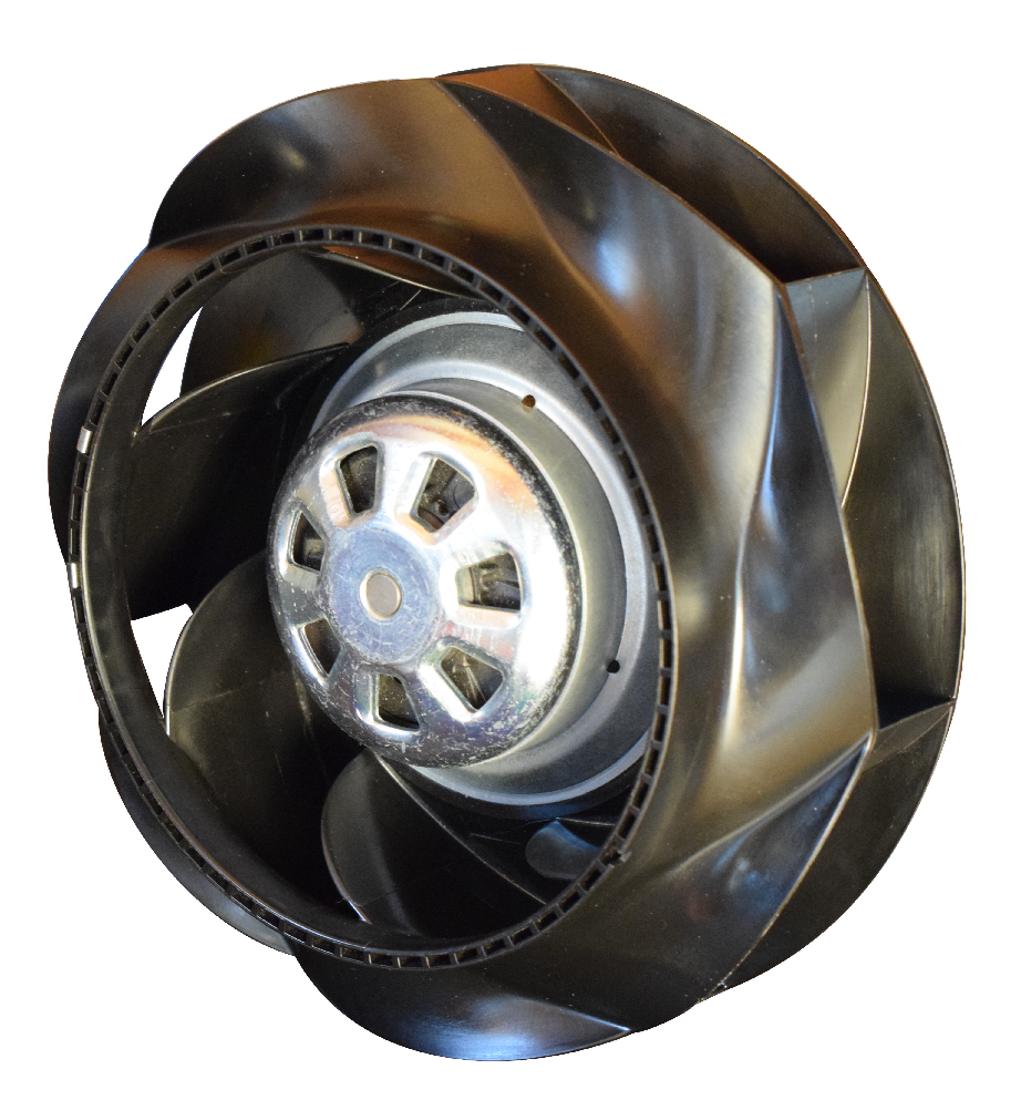
The fan analyzed here is a backward curved centrifugal fan designed by the ebm-papst GmbH & Co. KG. It is productively used for central ventilation systems in single and multifamily houses [22]. The impeller shown in Figure 1 has seven blades and an outer diameter of 190 mm. The nominal rotational speed is approximately 3635 rpm.
2.1.2. Fan Test Rig
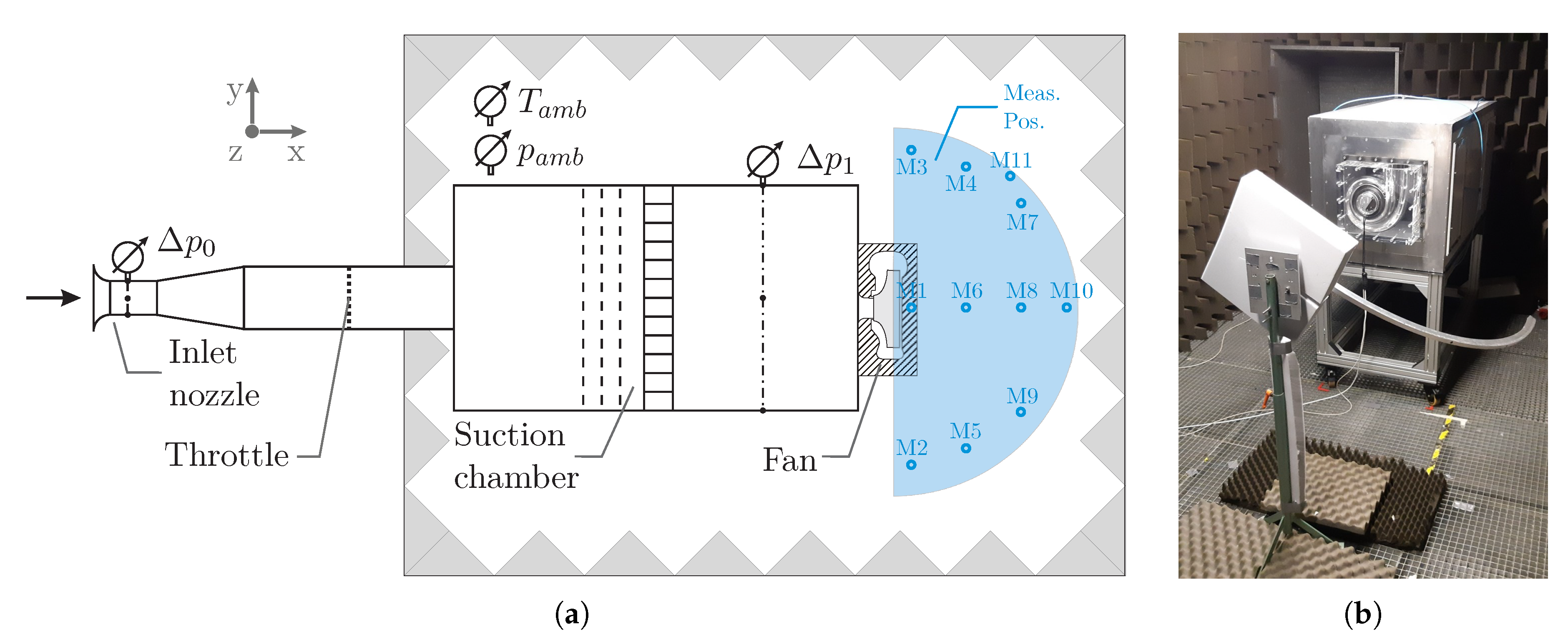
The experimental investigations were performed on the suction-side chamber fan test rig in the anechoic room of the Institute of Fluid Mechanics and Fluid Machinery at the University of Kaiserslautern. The test rig was developed according to DIN EN ISO 5801 and is schematically shown as top view in Figure 2a. A photograph of the measurement setup inside the anechoic room facility is shown in Figure 2b.
In total, the test rig includes an inlet section and a suction chamber. The inlet section consists of an inlet nozzle, a diffuser, a throttle, as well as a pipe section and is located outside of the anechoic room to decouple the expected noise emission of the throttle from that of the fan. In order to determine the volume flow, the differential pressure at the inlet nozzle was measured.
The differential pressure was acquired to calculate the pressure rise of the fan. Furthermore, the temperature and the ambient pressure in the anechoic room were recorded. They were used to set the physical conditions in the simulation. The sound pressure was measured at 11 measurement points on a hemisphere behind the fan, which is connected to the suction chamber. In Figure 2a they are presented as blue dots with numbers. Although the image shows only the projection of the measurement points on a horizontal plane, the points are measured at different heights. As in the simulation, the sound pressure and aerodynamic parameters were measured concurrently. The rotational speed was captured by a tacho signal which is integrated in the fan. The electrical power was measured by a power meter.
2.1.3. Aerodynamic Performance Measurements
The aerodynamics of a fan is quantified by the pressure rise and the efficiency , which are given in Equation (1). The values are calculated according to DIN EN ISO 5801. In the equations, the indices represent the evaluation position of the pressure. Here, 1 indicates the upstream and 2 the downstream of the fan. By considering the free blowing case, the ambient pressure can be assumed for the static pressure . Therefore, the pressure rise can then be taken directly from the measured differential pressure (see Figure 2a). As the torque could not be measured directly, the supplied power is estimated using the electric power , which is measured during the experiment and the motor efficiency , which is provided by the fan manufacturer ebm-papst GmbH & Co. KG.
2.1.4. Acoustic Measurements
The noise emission of a fan is determined by the sound pressure level as well as the total sound pressure level obtained from the frequency analysis. The quantities are defined according to DIN 45635-1 and are provided in Equation (2) for each measurement point i.
is the acoustic pressure at each measurement point i and frequency band j. is the reference sound pressure level an the number of frequency bands. Equation (3) is used to determine the average total sound pressure level over all measurement points . The evaluation of the frequency analysis of the sound pressure is done by the measurement software PAK 5.10 developed by Müller-BBM VibroAkustik Systems using the settings presented in Table 1.
2.2. Numerical Setup
2.2.1. Lattice Boltzmann Method
The commercial Lattice Boltzmann code SIMULIA PowerFLOW 6-2019-R2 developed by Dassault Systèmes was used to calculate the unsteady flow and the radiated acoustic of the centrifugal fan. In contrast to classical CFD methods, which are based on Navier Stokes equation and use a macroscopic view, the Lattice Boltzmann Method (LBM) relies on the Boltzmann equation and uses a mesoscopic approach. Since the number of molecules in a fluid is too high to model, the molecules were clustered to so-called particles and are represented by the velocity distribution function , which describes the probability of tracking particles at a specific location x in space with a certain velocity at time t.
The Boltzmann equation is a generally valid equation for determining the distribution function f. However, even with modern methods the Boltzmann equation given in tensor notation in Equation (4) cannot be solved.
stands for the above described velocity distribution function. The left side of Equation (4) contains the time and convective change of the distribution function as well as the change due to external forces . The right side of Equation (4) describes the change of the distribution function due to interaction of the particles and is called the collision term. Since the collision term is composed of a complex integral, it is approximated by a much simpler mathematical approach. Often, the so-called Bhatnagar-Gross-Krook (BGK) model according to Bhatnagar, Gross, and Krook [23] is used. The model assumes that every non-equilibrium condition leads to an equilibrium condition, cf. Equation (5).
describes the molecular collision frequency and indicates the number of transitions from non-equilibrium to equilibrium per time interval t. f stands for the non-equilibrium distribution and for the local equilibrium distribution. The equilibrium distribution is equal to the Maxwell distribution [24]. Using the BGK model [23] for the collision modeling and a Chapman–Enskog development [24,25], the Boltzmann Equation in Equation (4) recovers the Navier Stokes equation.
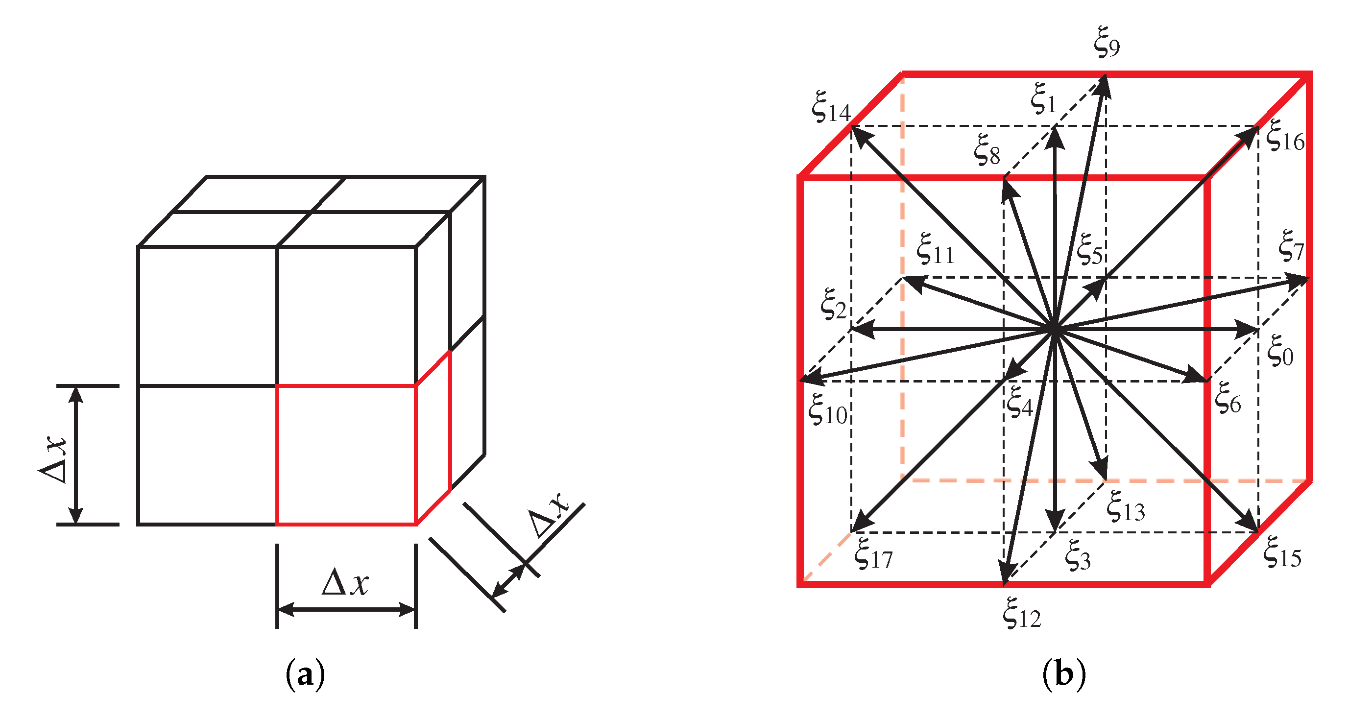
In order to solve the BGK Boltzmann equation numerically, a discretization in time, space, and velocity space is required. For a spatial discretization, the Cartesian space is split up into an equidistant mesh, cf. Figure 3a. Each mesh cell is called a lattice.
In addition to the spatial discretization, the velocity is discretized to predefined velocity directions. In the three-dimensional case, model D3Q19 is often used, which is also implemented in PowerFLOW 6-2019-R2. The model uses defined directions, which are indicated by in Figure 3b.
The discrete BGK Boltzmann equation presented in Equation (6) is called the Lattice BGK (LBGK).
The equation indicates that a calculation step consists of a transport step and a collision step . Algorithmically, these two steps are usually calculated separately for each velocity in each lattice per time step. In an explicit procedure the new distribution functions for the next time step can be determined.
With the known distribution function the macroscopic quantities of interest can be calculated by determining the moments. It is shown in Equation (7) exemplary for the calculation of macroscopic density and velocity.
The commercial LBM-Code PowerFLOW uses a so-called Very Large Eddy simulation (VLES) approach for the turbulence modeling. The resolvable scales are directly calculated and the unresolved scales are modeled. The modeling is done by a RNG turbulence model with a company-owned extension [27,28,29]. In addition to the turbulence modeling, a wall function is implemented in PowerFLOW. It is the logarithmic wall law, which has been additionally extended by pressure gradients, allowing the local surface friction to be determined [29]. The authors refer to [27,28,29] for further information.
2.2.2. Simulation Model
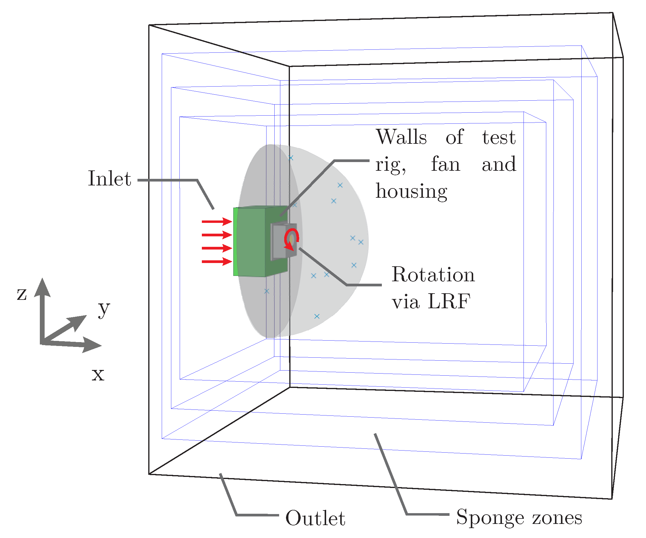
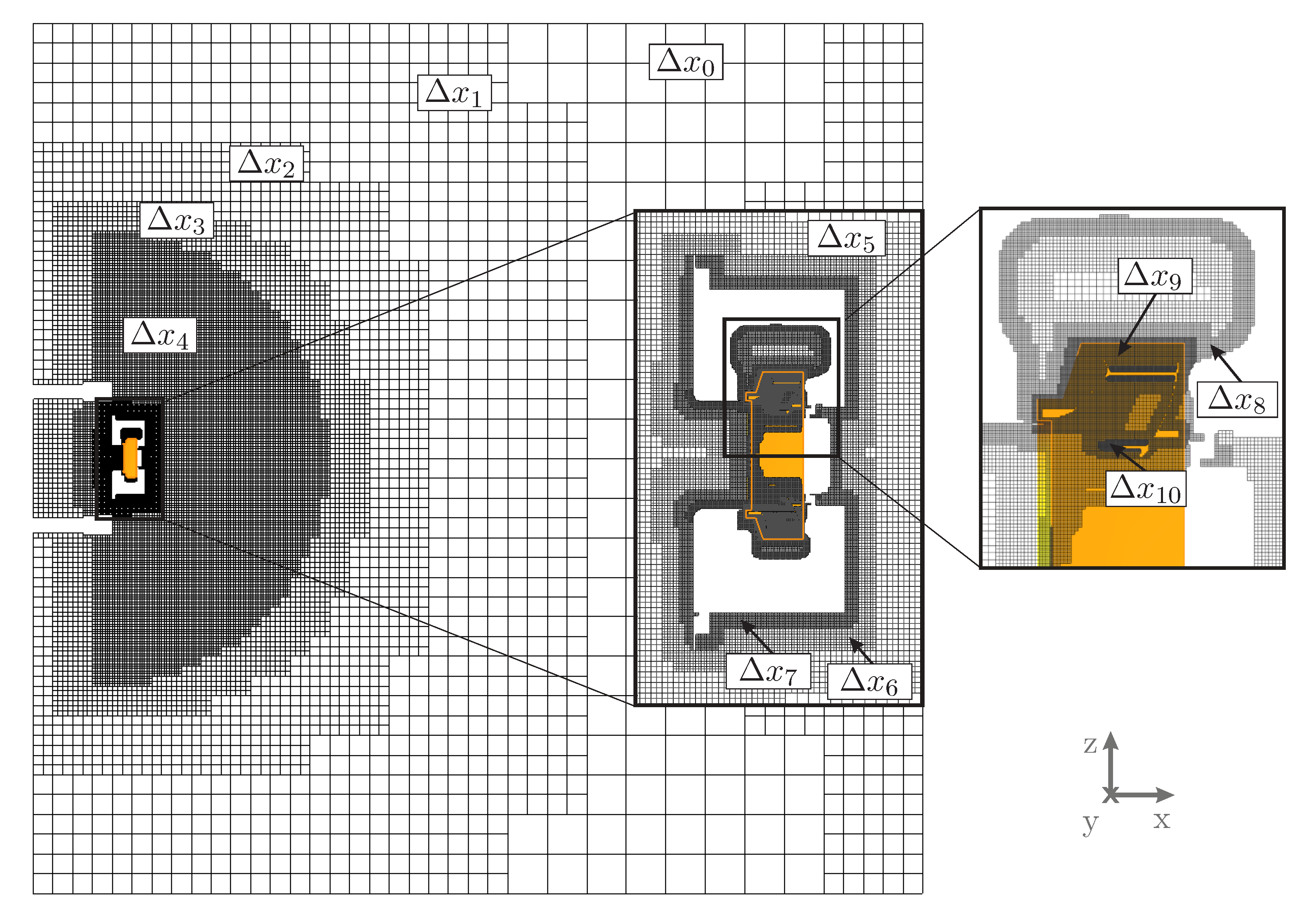
The simulation model shown in Figure 4 contains only the experimental setup starting from the pressure measurement location inside the suction chamber due to the lacking knowledge of the pressure losses of the screens and the honeycomb. As the acoustic measurement is acquired behind the fan, this simplification of the experimental setup should not influence the simulated results. The overall simulation area includes the anechoic room. Foams at the walls are modeled with so-called sponge zones, where the viscosity is increased over three layers. A velocity boundary is selected as the inlet boundary condition. The velocity corresponds to the mean velocity , which results from the measured volume flow Q, and can be calculated by using the continuity equation . The volume flow is varied between 70%, 100%, 120%, and 170% of the design volume flow . At the boundaries of the overall simulation area a pressure outlet is set according to the measured ambient pressure. The rotation of the fan is modeled by a local reference frame (LRF) using the sliding mesh approach and the rotating speed obtained by the measurements. The geometry of the LRF is shown in orange in Figure 5. The mesh setup without the housing was analyzed in detail in a previous work [26]. Here, an additional Variable Resolution (VR) region in the area of the blades and the housing had to be added. The smallest voxel size around the blades is and a total of 11 VR regions are set to generate the Cartesian mesh automatically by the solver (c.f. Figure 5).
The total number of volumetric cells is about and the number of surface elements is about . The simulation Mach number was set to the setting “same as experiment” and was thus . Based on the finest resolution and the Mach number, the time step is .
A total of of physical time, which corresponds to about 43 complete fan revolutions, was simulated. The pressure at the inlet and outlet as well as the torque were monitored during the simulation. The convergence was obtained after roughly , which is equal to around 19 fan revolutions.
3. Results and Discussion
3.1. Global Performance
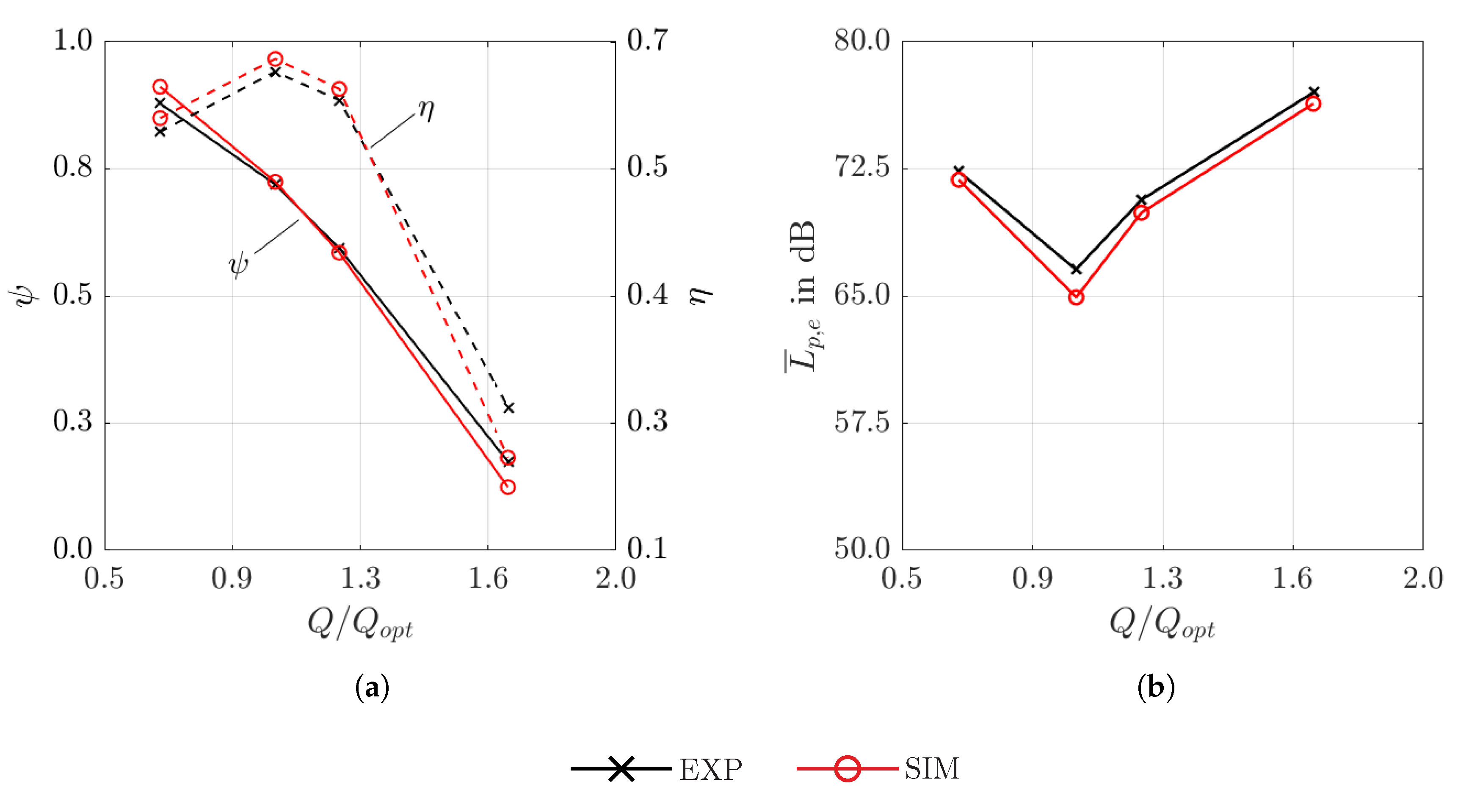
The fan aerodynamic performance curves in terms of pressure rise coefficient and efficiency are presented in Figure 6a. The pressure rise coefficient is defined as
and in case of the simulation it was derived as a mean value of the last 10 impeller revolutions. The static pressure is acquired on a plane of 1-by-1 , which is located 1 m downstream of the fan’s center. The static pressure is taken at the inlet. By comparing the values, there is a very good agreement between the measurement and the simulation with 0.5–3.5% deviation of pressure rise coefficient and in terms of efficiency of 0.7–2.5%. It is noticeable that the deviations increase towards higher volume flows. This behavior is in accordance with other publications regarding axial fans [5] due to a limited grid resolution affecting the results at high volume flow and high pressure conditions. An additional mesh study, of which the results are not shown here, confirm the assumption that a finer resolution for off-design conditions leads to even better result. However, the associated increase of the computing effort is not reasonable in terms of costs.
The acoustic characteristic in terms of total sound pressure is shown in Figure 6b. It is calculated from the acoustic spectra averaged over all measurement positions M1 to M11 in the range of 100–2500 Hz. Again, a very good agreement is achieved with a relative deviation of 0.2–2.4%. The deviations can be explained by reflections in the experiment, which cannot be modeled by the simulation due to the simplification of the model.
3.2. Acoustic Results
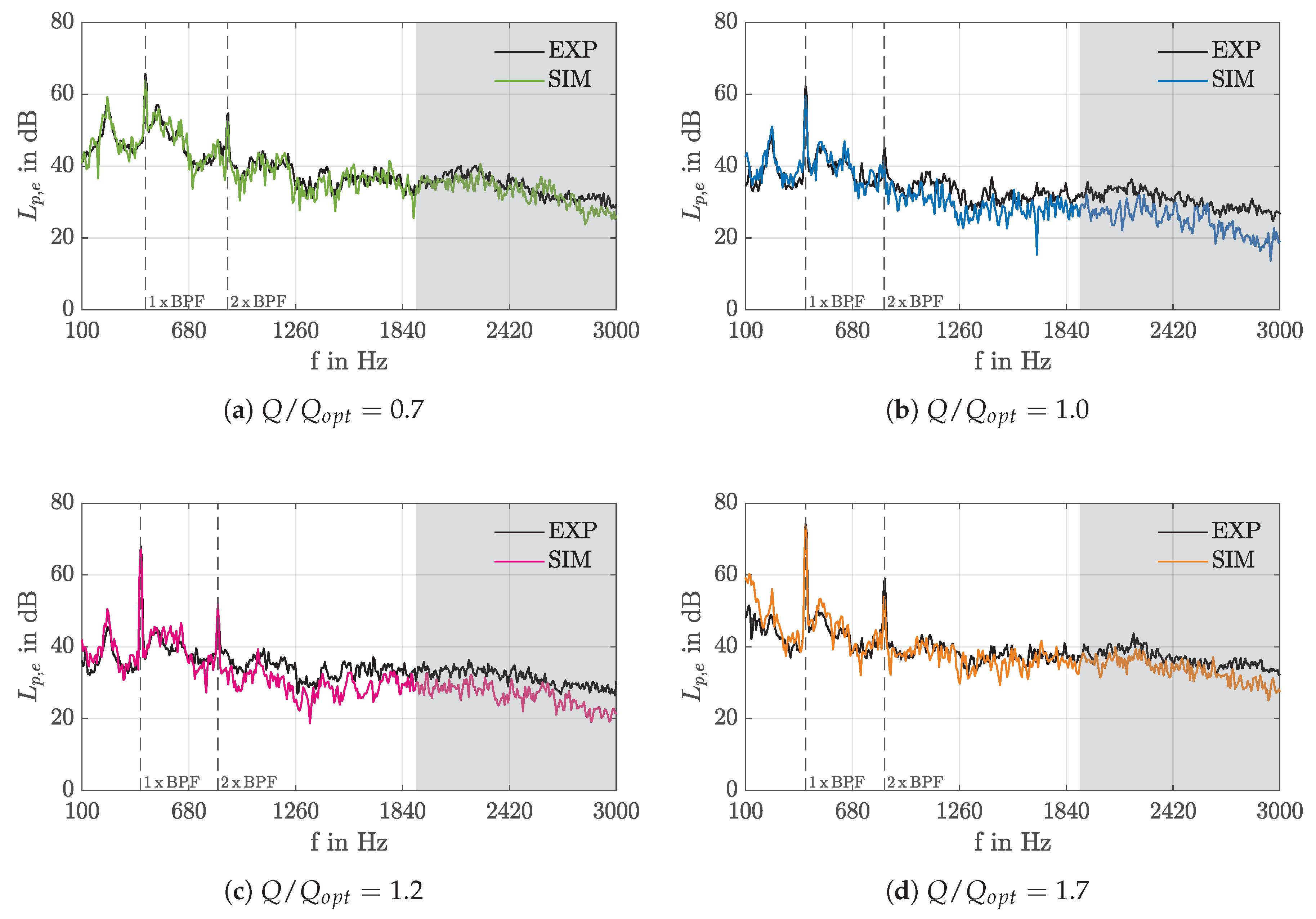
Acoustic narrow band spectra are presented in Figure 7. To evaluate the experiment and simulation, a time signal of s and a bandwidth of Hz is chosen. The first and second blade passing frequency (BPF) are marked as dotted lines. The simulation’s cut-off frequency is caused by the local mesh resolution of at the microphone positions and is marked in gray. It can be estimated by taking 14 points/wavelength [30]. An excellent agreement of the overall pressure level for all operating points in the range of 100 Hz to approximately 2400 Hz can be observed. Also, the sound pressure level at the first and second blade passing frequency can be predicted by the simulation.
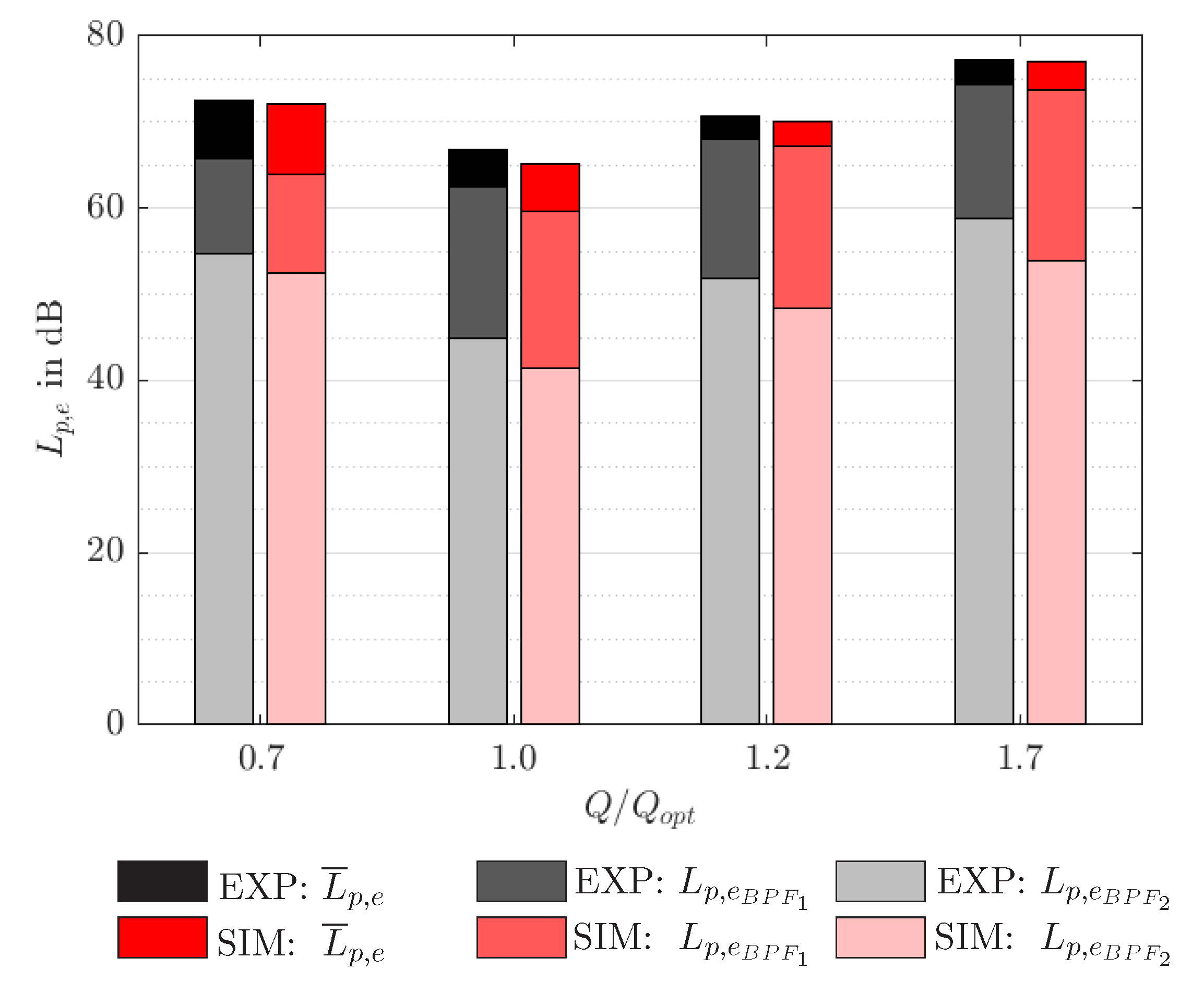
The comparison of the spectra for the different operating points shows that the broadband noise for and is lower than for the other two analyzed volume flows. With increased flow rate also the difference of the amplitude from BPF to the broadband is increasing. It can be assumed that the impact of the tonal noise on the total sound pressure level and the radiated noise is more dominant the higher the volume flow is. This is illustrated in more detail in Figure 8 where the total sound pressure level is depicted together with the first and second BPF peak level. The higher the flow rate, the lower is the difference between the total sound pressure level and the peak level of first BPF, resulting in a more tonal noise. The difference to the peak level of second BPF is relative constant over all operating points.
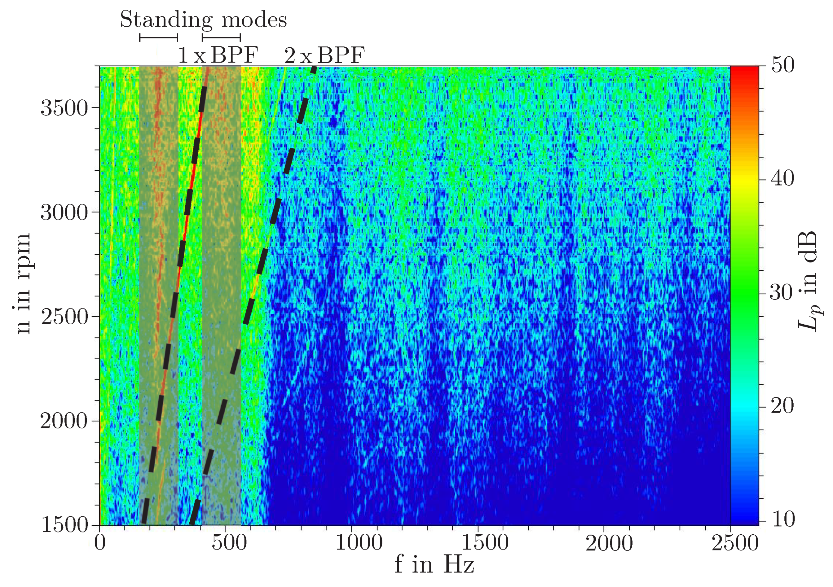
Especially tonal sound components are of high interest, as they are perceived by humans as more unpleasant [31]. Campbell diagrams show the sound pressure level as a function of the rotational speed and the frequency. They can be used to identify rotational dependent and independent tonal components of a noise source. Such a diagram is represented in Figure 9 for the operating point at microphone position MS10 and was produced by a experimental rotational speed test. It can be seen that there are both rotational and non-rotational related sound components leading more or less to tonal noise. As already shown in Figure 7, the blade passing frequency (1 × BPF) and its first harmonic (2 × BPF) are clearly visible, whereas higher harmonics cannot be separated so clear from the broadband noise. The non-rotational related noise components, which can be seen in the range of 250 Hz and 500 Hz, seems to be standing modes of the test bench. Beside the really good agreement of the amplitude of BPF between simulation and experiment it is noticeable that there is even a excellent agreement in the range of 250 Hz and 500 Hz (c.f. Figure 7). Because of this, it is assumed that beside rotational related and non-rotational related noise components like standing modes can be predicted by the LBM simulation. To verify this assumption the simulation was also performed beside the maximum rotational speed for two additional ones ( 3000 rpm and 1800 rpm). It can be seen that in the simulation the significant ranges at 250 Hz and 500 Hz are independent of rotational speed (c.f. Figure 10). Due to the decreasing of rotational speed, the sound pressure level is minimized. As in the experiment, in the simulation, the blade passing frequency and the first harmonic are in accordance with the fan’s rotational speed.
3.3. Flow Topology
The previous results show that the simulation is overall in good agreement with the experiment in terms of both aerodynamics and aeroacoustics. In contrast to experimental results, the numerical results can be used directly to obtain a more detailed understanding of the flow and afterwards also of the acoustic field.
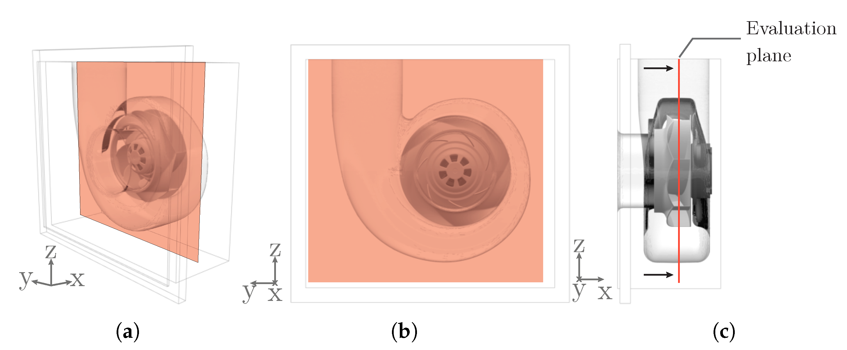
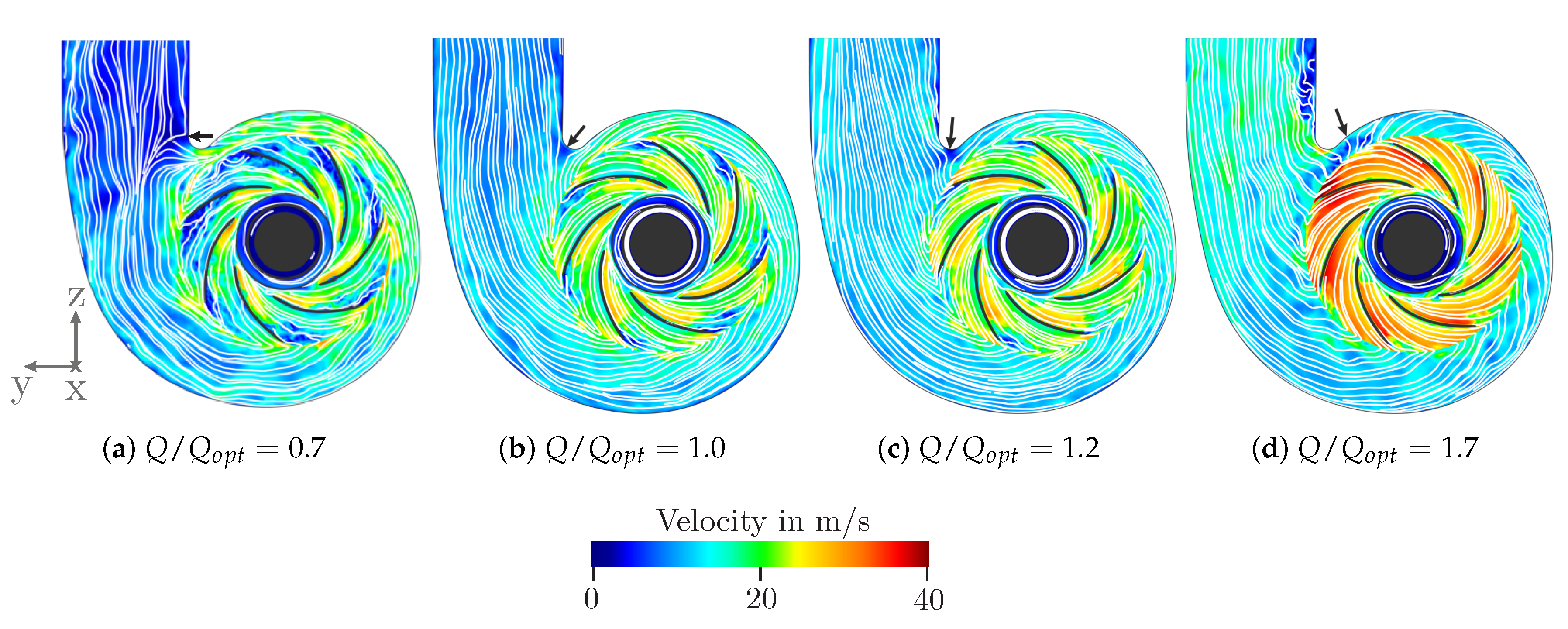
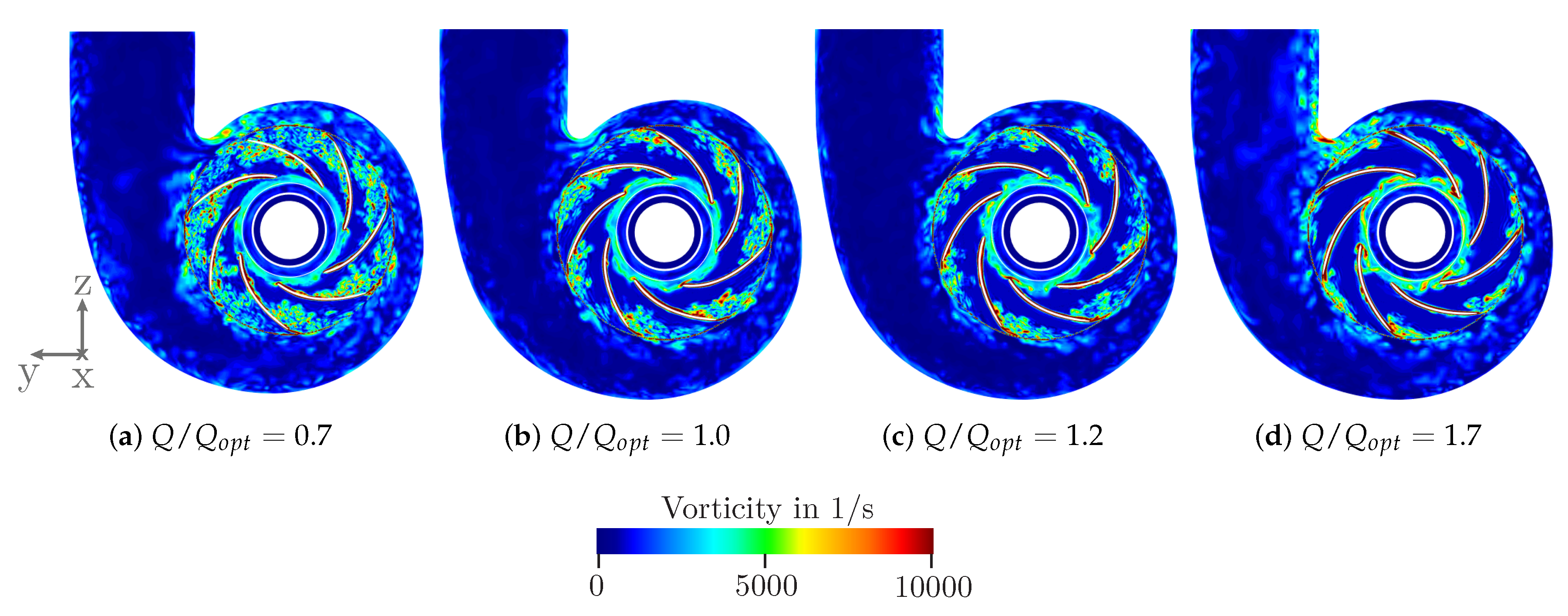
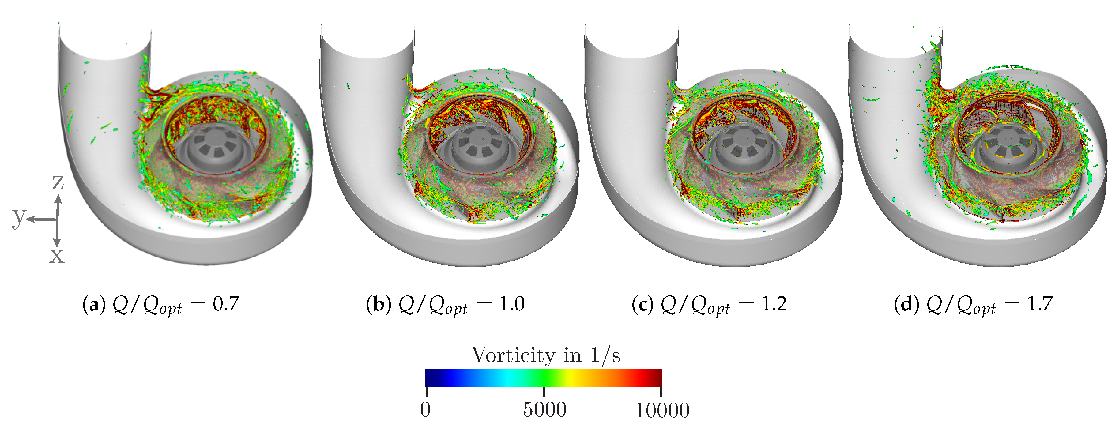
Through the mid-plane of the impeller, which is illustrated in Figure 11, the instantaneous velocity (c.f. Figure 12) and the instantaneous vorticity field (c.f. Figure 13) are shown. Also, the streamlines projected to the plane are depicted as white lines in Figure 12. The velocity with respect to the containing reference frame is used for the velocity field. With an increasing flow rate, the fluid leaves the impeller more and more radially. For the highest flow rate, the flow is fully attached to the blades and the main source of vorticity is in the wake of the impeller’s trailing edge. The more the volume flow is reduced, the stronger the flow is detached from the blades inside of the blade passage. By characterizing the position of the separation, the main source of the vortex formation can be identified by the vorticity. It is noticeable that the stagnation point, marked by the black arrow in Figure 12, changes depending on the flow rate, which Marsan also remarked on in his results of URANS simulation of a radial blower [32]. It can be observed that at partial load the stagnation point is shifted downstream of the tongue towards the outlet. At the design point, it is located at the tongue. In case of overload it moves downstream along the spiral housing starting at the tongue. It could be that there is a correlation between the flow towards the tongue and the developing of noise emission. For instance, at the design point the flow towards the tongue seems to be optimum. This matches where the lowest sound pressure level could be found (cf. Figure 6b).
The detachment at the tongue and also at the impeller’s leading edge resulting in vortex formation in the flow field can be identified even in more detail by the criterion shown in Figure 14. From this, it is assumed that the vortex formation and the blade passage flow influence the acoustics of the fan and may also be responsible for noise sources. In the following investigations, these assumptions are verified by means of even more detailed examination of the acoustic flow field.
3.4. Analysis of the Acoustic Field
The following paragraph is focused on the unsteady phenomena in the frequency band around BPF and between 100–2500 Hz. Zones of high pressure fluctuations indicates areas of noise sources. For that the power spectra of the fluid volume as well as the impeller’s and housing’s surface are considered.
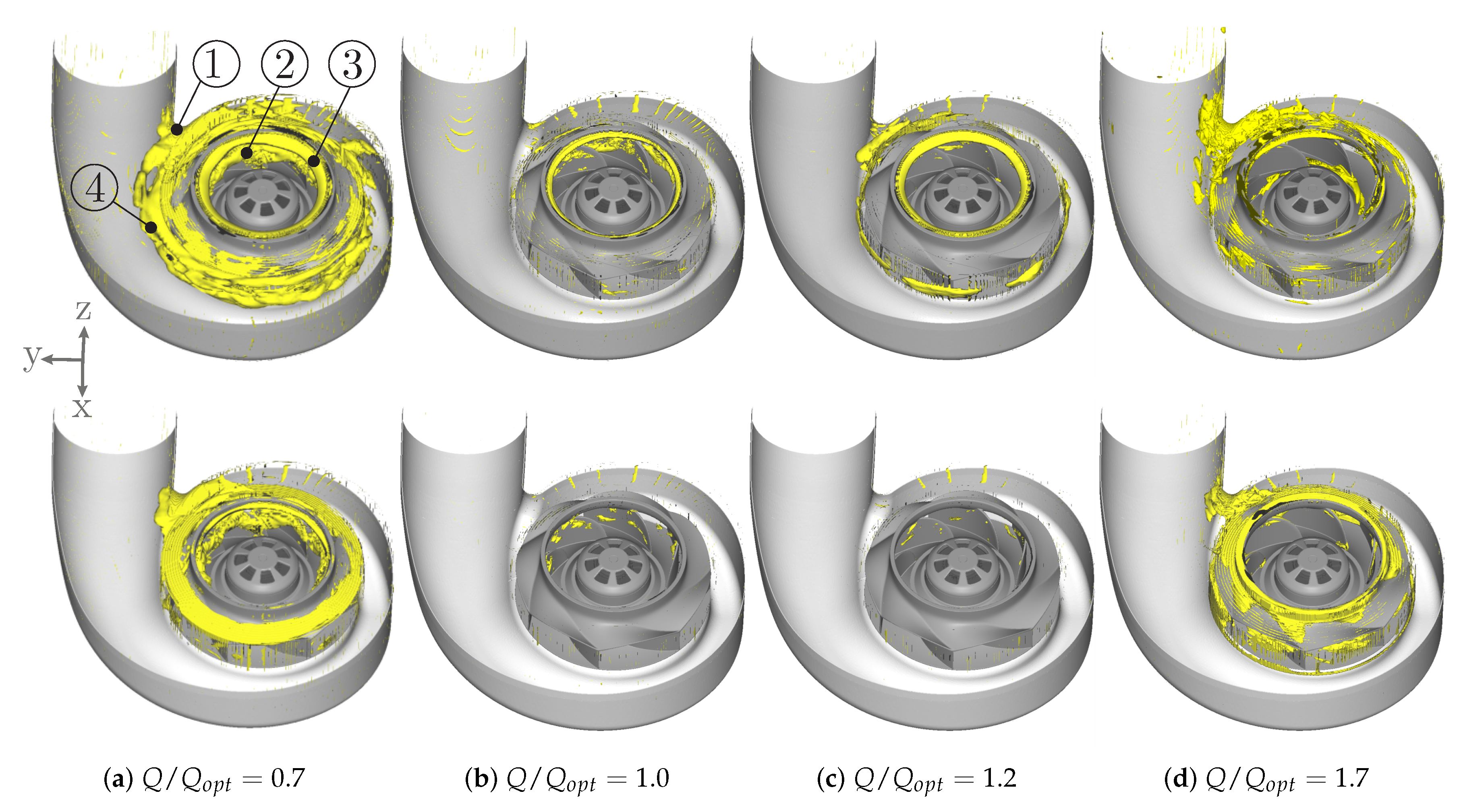
In Figure 15 an isosurface of the pressure fluctuations is depicted for all analyzed operating points as isometric view. The top row shows the results filtered around BPF with values higher than 115 dB and the bottom row for the broadband with values higher than dB. As the overall sound pressure level for the operating points and is much lower than for the other two operating points the isosurfaces are not as intensively developed. Four significant areas are identified, which are considered as main noise sources and are marked in Figure 15 for operating point representative for all other operating points:
- ①
- Tongue area;
- ②
- Blade passage;
- ③
- Gap between impeller and housing;
- ④
- Wake of the impeller’s trailing edge.
These areas are in accordance with the assumptions from the velocity and vorticity field made in Section 3.3. It seems that the hydrodynamic and the acoustic field are linked directly. Since the highest values of operating point and filtered around the BPF can be found in the area of the gap between impeller and housing, these areas seem to influence the amplitude of BPF most. The maximum values of and are found at the tongue which therefore appears here to have the main influence. In the broadband the maximum values can be found for all operating points at the tongue and in the blade passage.
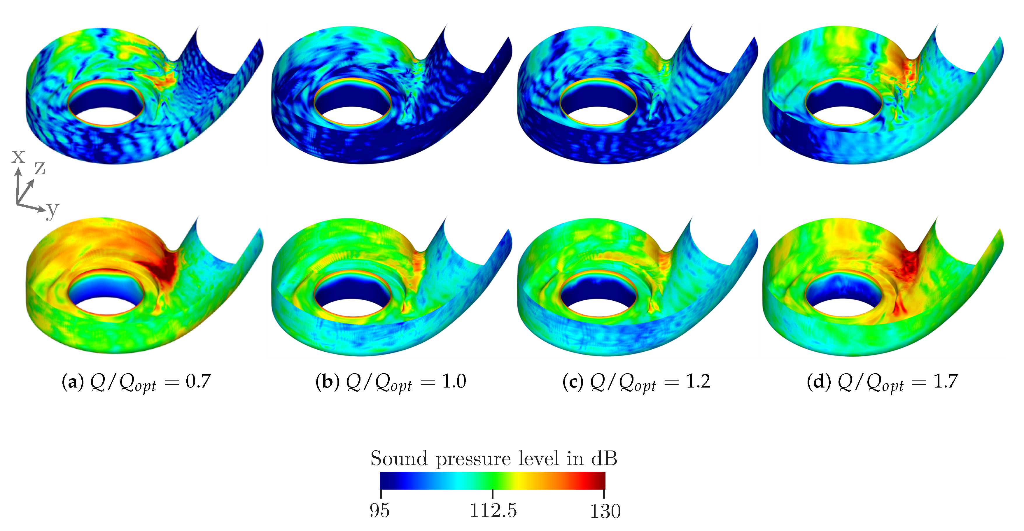
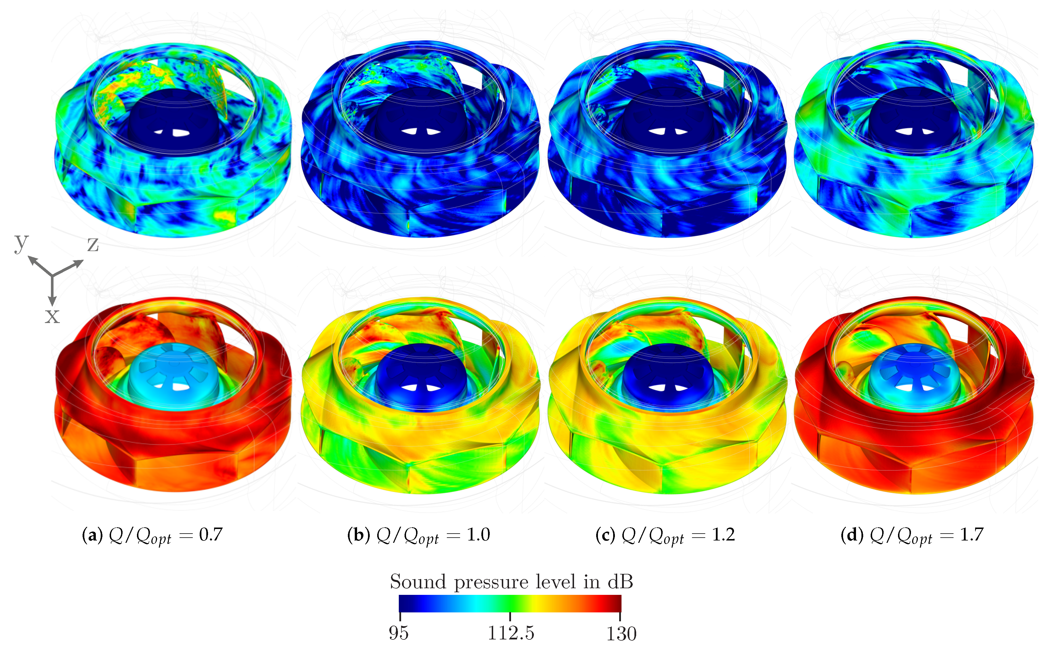
The four significant areas can also be identified by the wall sound pressure level of housing and impeller, which are illustrated in Figure 16 and Figure 17. The highest values in the frequency range around BPF for and can again be found in the area of the tongue. High values are also identified in the area of the nozzle and on the blades. The first one can be directly associated with the noise source in the area of the gap between the impeller and housing and the latter one with the blades passage noise source. For and maximum values of wall pressure fluctuation in the range of BPF are also at the nozzle. In the broadband the highest values can be found for all operating points at the tongue, the nozzle and the blades.
Looking in more detail at the noise sources, they can be associated with flow phenomena: The noise source around the tongue can be related to the detachment from the tongue, as already demonstrated in Figure 12 and Figure 13. The interaction of the impeller’s wake flow with the tongue is also known to be the cause of the noise source around the tongue, especially for the tonal sound [33]. Detachments from the impeller’s leading edge and the associated interaction of the vortexes shown in Figure 14 seems to be related to the noise sources inside of the blade passage. The noise source around the gap can be associated by the interaction of the main flow with flow through the gap [15,16].
4. Conclusions and Outlook
The aerodynamic and aeroacoustic of a centrifugal fan with spiral housing built into a suction fan test rig could be successfully simulated in a direct approach by the Lattice Boltzmann Method using the commercial LBM-code SIMULIA PowerFLOW 6-2019-R2. Four different operating points were analyzed, covering partial load and design point as well as the overload and heavy overload of the fan curve. Except for extreme off-design conditions, the fan’s performance in terms of pressure rise coefficient and efficiency is well captured in these simulations. Excellent agreement is achieved with the acoustic pressure spectra and total sound pressure level.
The simulation results were also used to analyze the flow and acoustic field of the centrifugal fan. Differences in the flow pattern of the different operating points could be shown by the vorticity and the velocity and are in alignment with the performance curves. Using acoustic analysis techniques like the filtered pressure fluctuations on the walls and in the flow field it is possible to localize the noise-generating flow features. Four significant areas are identified, which are considered as main noise sources: the tongue area, the blade passage, the gap between the impeller, and the housing as well as the wake of the impeller’s trailing edge. By comparing of the flow structures and noise sources, it is suggested that the noise sources originate from detachments from leading and trailing edge and the tongue as well as from the interaction of the impeller’s wake with the tongue and the main flow with the flow through the gap. These noise sources of centrifugal fans and their origin have already been analyzed by conventional methods using acoustic models. This contribution demonstrates that the Lattice Boltzmann Method, which is able to calculate the aeroacoustic directly, is an good alternative approach to conventional methods. In further investigations, the results could be used to understand the noise source origin and the general noise-generating mechanisms of centrifugal fan in more detail. Examining the results at all the significant frequency bands could help to assign the main noise sources to the different frequencies.
Author Contributions
The authors contributed equally to the paper. All authors have read and agreed to the published version of the manuscript.
Funding
The research project was funded by the Federal Ministry for Economic Affairs and Energy (BMWi) grant number IGF.-Nr. 19382 N/1 through the German Federation of Industrial Research Associations Otto von Guericke e.V. (AiF) on the basis of a decision of the “German Bundestag”.
Acknowledgments
We thank the member companies of the “Forschungsvereinigung für Luft- und Trocknungstechnik e.V.” (Research Association for Air and Drying Technology) (FLT) for the material and project-accompanying support. The simulations were conducted on the high performance cluster “Elwetritsch” at Univercity of Kaiserslautern, which is part of the Alliance of High Performance Rhineland-Palatinate (AHRP). Finally, the authors thank Dassault Systèmes for providing PowerFLOW licenses and support.
Conflicts of Interest
The authors declare no conflict of interest.
Abbreviations
| BPF | Blade passing frequency |
| CFD | Computational Fluid Dynamics |
| EXP | Experiment |
| FWH | Ffowcs Williams and Hawkings |
| LBM | Lattice Boltzmann Method |
| LES | Large Eddy Simulation |
| LRF | Local Reference Frame |
| RANS | Reynolds Averaged Navier Stokes |
| SIM | Simulation |
| URANS | Unsteady Reynolds Averaged Navier Stokes |
| VLES | Very Large Eddy Simulation |
| VR | Variable Resolution |
| Latin symbols | |
| c | Velocity |
| D | Outer diameter of impeller |
| f | Frequency |
| f | Velocity distribution function |
| Sound pressure level | |
| MACH Number | |
| n | Rotational speed |
| Total number of measurement points | |
| Total number of frequency bands | |
| Electrical power | |
| p | Pressure |
| Reference sound pressure | |
| Q | Volume flow |
| u | Circumferential velocity at impeller’s outlet |
| Cartesian coordinates | |
| Greek symbols | |
| p | Pressure rise |
| x | Lattice size |
| Density | |
| Efficiency | |
| Particle velocity | |
| Collision frequency | |
| Subscripts | |
| 1 | Inflow |
| 2 | Outflow |
| amb | Ambient |
| char | Characteristic |
| eq | Equilibrium |
| i | Measurement point |
| j | Frequency band |
| m | Motor |
References
- Hänel, D. Molekulare Gasdynamik: Einführung in die Kinetische Theorie der Gase und Lattice-Boltzmann-Methoden; Springer: Berlin/Heidelberg, Germany, 2004. [Google Scholar]
- Perot, F.; Kim, M.S.; Moreau, S.; Neal, D. Investigation of the Flow Generated by an Axial 3-Blade Fan. In Proceedings of the 13th International Symposium on Transport Phenomena and Dynamics of Rotating Machinery (ISROMAC-13), Honolulu, HI, USA, 4–7 April 2010; pp. 198–204. [Google Scholar]
- Pérot, F.; Moreau, S.; Kim, M.S.; Henner, M.; Neal, D. Direct aeroacoustics predictions of a low speed axial fan. In Proceedings of the 16th AIAA/CEAS Aeroacoustics Conference, Stockholm, Sweden, 7–9 June 2010; pp. 1–15. [Google Scholar]
- Lallier-Daniels, D.; Moreau, S.; Sanjose, M.; Pérot, F. Numerical Analysis of Axial Fans for Performance and Noise Evaluation Using the Lattice Boltzmann Method. In Proceedings of the 21st Annual Conference of the CFD Society of Canada, Sherbrooke, QC, Canada, 6–9 May 2013; pp. 1–15. [Google Scholar]
- Pérot, F.; Kim, M.S.; Moreau, S.; Henner, M. Axial fan noise aeroacoustics predictions and inflow effect on tonal noise using LBM. In Proceedings of the 21st Annual Conference of the CFD Society of Canada, Sherbrooke, QC, Canada, 6–9 May 2013; pp. 1–9. [Google Scholar]
- Zhu, T.; Sturm, M.; Carolus, T.; Neuhierl, B.; Perot, F. Experimental and numerical investigation of tip clearance noise of an axial fan using a lattice Boltzmann method. In Proceedings of the 21st International Congress on Sound and Vibration, Beijing, China, 13–17 July 2014; pp. 1–8. [Google Scholar]
- Sturm, M.; Sanjosé, M.; Moreau, S.; Carolus, T. Aeroacoustic simulation of an axial fan including the full test rig by using the lattice Boltzmann method. In Proceedings of the Fan 2015, International Conference on Fan Noise, Technology and Numerical Methods, Lyon, France, 15–17 April 2015; pp. 1–12. [Google Scholar]
- Marsan, A.; Lallier-Daniels, D.; Sanjose, M.; Mann, A.; Moreau, S. Tip leakage flow and its implication on the acoustic signature of a low-speed fan. In Proceedings of the Fan 2018, International Conference on Fan Noise, Aerodynamics, Applications and Systems, Darmstadt, Germany, 18–20 April 2018. [Google Scholar]
- Magne, S.; Sanjosé, M.; Moreau, S.; Berry, A. Numerical optimization of fan tonal noise control using acoustic modulation of slowly-rotating obstructions. In Proceedings of the 20th AIAA/CEAS Aeroacoustics Conference, Atlanta, GA, USA, 16–20 June 2014; pp. 1–12. [Google Scholar]
- Moreau, S.; Sanjosé, M.; Magne, S. Optimization of tonal noise control with flow obstruction. J. Sound Vib. 2018, 437, 264–275. [Google Scholar] [CrossRef]
- Piellard, M.; Coutty, B.; Le Goff, V.; Vidal, V.; Perot, F. Direct aeroacoustics simulation of automotive engine cooling fan system: Effect of upstream geometry on broadband noise. In Proceedings of the 20th AIAA/CEAS Aeroacoustics Conference, Atlanta, GA, USA, 16–20 June 2014; pp. 1–16. [Google Scholar]
- Lallier-Daniels, D.; Piellard, M.; Coutty, B.; Moreau, S. Aeroacoustic Study of an Axial Ring Fan using Lattice-Boltzmann Simulations and the Ffowcs-Williams and Hawkings Analogy. In Proceedings of the 16th International Symposium on Transport Phenomena and Dynamics of Rotating Machinery (ISROMAC-16), Honolulu, HI, USA, 10–15 April 2016. [Google Scholar]
- Pérot, F.; Kim, M.S.; Wada, K.; Norisada, K.; Kitada, M.; Hirayama, S.; Sakai, M.; Imahigasi, S.; Sasaki, N. HVAC blower aeroacoustics predictions based on the Lattice Boltzmann Method. In Proceedings of the ASME/JSME/KSME Joint Fluids Engineering Conference, Hamamatsu, Japan, 24–29 July 2011; pp. 921–929. [Google Scholar]
- Norisada, K.; Sakai, M.; Ishiguro, S.; Kawaguchi, M.; Perot, F.; Wada, K. HVAC Blower Aeroacoustic Predictions. In Proceedings of the SAE 2013 World Congress & Exhibition, Detroit, MI, USA, 16–18 April 2013. [Google Scholar]
- Le Goff, V.; Le Hénaff, B.; Piellard, M.; Pihet, D.; Coutty, B. Toward a full digital apprach for aeroacoustics evaluation of automotive engine cooling fans and HVAC blowers. In Proceedings of the Fan 2015, International Conference on Fan Noise, Technology and Numerical Methods, Lyon, France, 15–17 April 2015. [Google Scholar]
- Le Goff, V.; Mann, A.; Le Hénaff, B.; Pihet, D. A Digital Approach to the Aeroacoustic Evaluation of HVAC Blowers. ATZ Worldw. 2017, 119, 50–53. [Google Scholar]
- Pérot, F.; Kim, M.S.; Le Goff, V.; Carniel, X.; Goth, Y.; Chassaignon, C. Numerical optimization of the tonal noise of a backward centrifugal fan using a flow obstruction. Noise Control. Eng. J. 2013, 61, 307–319. [Google Scholar] [CrossRef] [Green Version]
- Pain, R.; Le Goff, V.; Pérot, F.; Shestopalov, A.; Learned Boucher, A.; Kim, M.S.; Carniel, X.; Goth, Y.; Chassaignon, C. Numerical optimization of the tonal noise of a backward centrifugal fan using a flow obstruction. Part II: Flow Obstruction Optimization. In Proceedings of the Fan 2015, International Conference on Fan Noise, Technology and Numerical Methods, Lyon, France, 15–17 April 2015. [Google Scholar]
- Magne, S.; Sanjosé, M.; Moreau, S.; Berry, A.; Gerard, A. Tonal noise control of centrifugal fan using flow obstructions—Experimental and numerical approaches. In Proceedings of the 19th AIAA/CEAS Aeroacoustics Conference, Berlin, Germany, 27–29 May 2013; pp. 1–13. [Google Scholar]
- Sanjose, M.; Moreau, S. Direct noise prediction and control of an installed large low-speed radial fan. Eur. J. Mech. B Fluids 2017, 61, 235–243. [Google Scholar] [CrossRef] [Green Version]
- Schäfer, R.; Böhle, M. Validation of the Lattice Boltzmann Method for the simulation of the aerodynamics and aeroacoustics in a centrifugal fan. In Proceedings of the 18th International Symposium on Transport Phenomena and Dynamics of Rotating Machinery, Online Event, 23–26 November 2020; pp. 1–8. [Google Scholar]
- ebm-papst Mulfingen GmbH & Co. KG. Radialventilator: RadiCal im Spiralgehäuse; ebm-papst Mulfingen GmbH & Co. KG: Mulfingen, Germany, 2017. [Google Scholar]
- Bhatnagar, P.L.; Gross, E.P.; Krook, M. A model for collision processes in gases. I. Small amplitude processes in charged and neutral one-component systems. Phys. Rev. 1954, 94, 511–525. [Google Scholar] [CrossRef]
- Guo, Z.; Shu, C. Lattice Boltzmann Method and Its Application in Engineering. In Advances in Computational Fluid Dynamics; World Scientific Publishing Company: Singapore, 2013; Volume 3. [Google Scholar]
- Succi, S. The Lattice Boltzmann Equation: For Fluid Dynamics and Beyond; Oxford Science Publications: Oxford, UK; Clarendon Press: Oxford, UK, 2001. [Google Scholar]
- Schäfer, R.; Böhle, M. Influence of the Mesh Size on the Aerodynamic and Aeroacousticsof a Centrifugal Fan using the Lattice Boltzmann Method. In Proceedings of the ICA 2019 and EAA Euroregio, Aachen, Germany, 9–13 September 2019; pp. 1882–1889. [Google Scholar]
- Fares, E.; Noelting, S. Unsteady Flow Simulation of a High-Lift configuration using a Lattice Boltzmann Approach. In Proceedings of the 49th AIAA Aerospace Sciences Meeting including the New Horizons Forum and Aerospace Exposition, Orlando, FL, USA, 4–7 January 2011. [Google Scholar]
- Chen, H.; Kandasamy, S.; Orszag, S.; Shock, R.; Succi, S.; Yakhot, V. Extended Boltzmann kinetic equation for turbulent flows. Science (N. Y.) 2003, 301, 633–636. [Google Scholar] [CrossRef] [PubMed]
- Kotapati, R.; Keating, A.; Kandasamy, S.; Duncan, B.; Shock, R.; Chen, H. The Lattice-Boltzmann-VLES Method for Automotive Fluid Dynamics Simulation, a Review. In Proceedings of the Symposium on International Automotive Technology, Pune, India, 21–23 January 2009. [Google Scholar]
- Brès, G.; Perot, F.; Freed, D. Properties of the Lattice Boltzmann Method for Acoustics. In Proceedings of the 15th AIAA/CEAS Aeroacoustics Conference, Miami, FL, USA, 11–13 May 2009; pp. 1–11. [Google Scholar]
- Gerard, A.; Besombes, M.; Berry, A.; Masson, P.; Moreau, S. Tonal noise control from centrifugal fans using flow control obstructions. Noise Control. Eng. J. 2013, 61, 381–388. [Google Scholar] [CrossRef]
- Marsan, A.; Moreau, S. Aeroacoustic Analysis of the Tonal Noise of a Large-Scale Radial Blower. J. Fluids Eng. 2018, 140, 021103. [Google Scholar] [CrossRef]
- Velarde-Suárez, S.; Ballesteros-Tajadura, R.; Pablo Hurtado-Cruz, J.; Santolaria-Morros, C. Experimental determination of the tonal noise sources in a centrifugal fan. J. Sound Vib. 2006, 295, 781–796. [Google Scholar]
Figure 1.
Photograph of the investigated centrifugal fan depicted without the spiral housing.

Figure 2.
Schematic view of the fan test rig as top view (a) and photograph of the measurement setup inside the anechoic room facility (b).
Figure 2.
Schematic view of the fan test rig as top view (a) and photograph of the measurement setup inside the anechoic room facility (b).

Figure 3.
Spatial discretization (a) and model D3Q19 of velocity discretization (b) [26].
Figure 3.
Spatial discretization (a) and model D3Q19 of velocity discretization (b) [26].

Figure 4.
Schematic view of the simulation model and the boundary conditions.

Figure 5.
Mesh topology, the orange area indicates the local reference frame (LRF) region.

Figure 6.
Pressure rise coefficient and efficiency (a) as well as total sound pressure (b) as function of volume flow rate
Figure 6.
Pressure rise coefficient and efficiency (a) as well as total sound pressure (b) as function of volume flow rate

Figure 7.
Acoustic spectra averaged over measurement positions M1 to M11 (shown in Figure 2a); the simulation’s cut-off frequency is marked in gray, the first (1 × BPF) and second (2 × BPF) blade passing frequency are indicated by dotted lines. BPF—blade passing frequency.
Figure 7.
Acoustic spectra averaged over measurement positions M1 to M11 (shown in Figure 2a); the simulation’s cut-off frequency is marked in gray, the first (1 × BPF) and second (2 × BPF) blade passing frequency are indicated by dotted lines. BPF—blade passing frequency.

Figure 8.
Total sound pressure level in comparison to the first and second BPF peak levels and extracted from the acoustic spectra averaged over measurement positions M1 to M11 for experiment (EXP) and simulation (SIM).
Figure 8.
Total sound pressure level in comparison to the first and second BPF peak levels and extracted from the acoustic spectra averaged over measurement positions M1 to M11 for experiment (EXP) and simulation (SIM).

Figure 9.
Campbell diagram of rotational speed test for at microphone position M10 determined by experiment.
Figure 9.
Campbell diagram of rotational speed test for at microphone position M10 determined by experiment.

Figure 10.
Acoustic narrow band spectra of variation of rotational speed for at microphone position M10 determined by simulation.
Figure 10.
Acoustic narrow band spectra of variation of rotational speed for at microphone position M10 determined by simulation.

Figure 11.
Illustration of the impeller and housing in gray and the evaluation plane through the center of the impeller in red as isometric view (a), in x-direction (b) and y-direction (c); the black arrows in (c) indicate the viewing direction.
Figure 11.
Illustration of the impeller and housing in gray and the evaluation plane through the center of the impeller in red as isometric view (a), in x-direction (b) and y-direction (c); the black arrows in (c) indicate the viewing direction.

Figure 12.
Instantaneous velocity with respect to the containing reference frame superimposed with projected streamlines on the plane shown in Figure 11; the black arrow mark the stagnation point.
Figure 12.
Instantaneous velocity with respect to the containing reference frame superimposed with projected streamlines on the plane shown in Figure 11; the black arrow mark the stagnation point.

Figure 13.
Instantaneous vorticity field on the plane shown in Figure 11.
Figure 13.
Instantaneous vorticity field on the plane shown in Figure 11.

Figure 14.
Instantaneous isosurface of values lower than colored by vorticity magnitude.

Figure 15.
Isosurface of the pressure fluctuation filtered around BPF with values higher than 115 dB (top) and in a broadband range of 100–2500 Hz with values higher than dB (bottom); the numbers mark the identified main noise source locations: 1 tongue area; 2 blade passage; 3 gap between impeller and housing; 4 wake of the impeller’s trailing edge.

Figure 16.
Wall sound pressure level of housing filtered around BPF (top) and in a broadband range of 100–2500 Hz (bottom).
Figure 16.
Wall sound pressure level of housing filtered around BPF (top) and in a broadband range of 100–2500 Hz (bottom).

Figure 17.
Wall sound pressure level of impeller filtered around BPF (top) and in a broadband range of 100–2500 Hz (bottom).
Figure 17.
Wall sound pressure level of impeller filtered around BPF (top) and in a broadband range of 100–2500 Hz (bottom).


Table 1.
Acoustic spectral analysis parameters.
| Parameters | Settings |
|---|---|
| Sampling rate | 51,200 Hz |
| Signal length | 10 s |
| Bandwidth | 6.25 Hz |
| Window | Hanning |
| Overlapping of windows | 50% |
| Averaging | linear |
© 2020 by the authors. Licensee MDPI, Basel, Switzerland. This article is an open access article distributed under the terms and conditions of the Creative Commons Attribution (CC BY) license (http://creativecommons.org/licenses/by/4.0/).
Share and Cite
MDPI and ACS Style
Schäfer, R.; Böhle, M. Validation of the Lattice Boltzmann Method for Simulation of Aerodynamics and Aeroacoustics in a Centrifugal Fan. Acoustics 2020, 2, 735-752. https://0-doi-org.brum.beds.ac.uk/10.3390/acoustics2040040
AMA Style
Schäfer R, Böhle M. Validation of the Lattice Boltzmann Method for Simulation of Aerodynamics and Aeroacoustics in a Centrifugal Fan. Acoustics. 2020; 2(4):735-752. https://0-doi-org.brum.beds.ac.uk/10.3390/acoustics2040040
Chicago/Turabian StyleSchäfer, Rebecca, and Martin Böhle. 2020. "Validation of the Lattice Boltzmann Method for Simulation of Aerodynamics and Aeroacoustics in a Centrifugal Fan" Acoustics 2, no. 4: 735-752. https://0-doi-org.brum.beds.ac.uk/10.3390/acoustics2040040