
Aerodynamic and Aeroacoustic Analysis of a Harmonically Morphing Airfoil Using Dynamic Meshing


1
Propulsion Engineering Centre, School of Aerospace Transport and Manufacturing, Cranfield University, Bedfordshire MK43 0AL, UK
2
Department of Engineering Design and Mathematics, University of the West of England, Coldharbour Lane, Frenchay, Bristol BS16 1QY, UK
*
Author to whom correspondence should be addressed.
Acoustics 2021, 3(1), 177-199; https://0-doi-org.brum.beds.ac.uk/10.3390/acoustics3010013
Submission received: 19 December 2020
/
Revised: 7 February 2021
/
Accepted: 2 March 2021
/
Published: 6 March 2021
Abstract
:This work explores the aerodynamic and aeroacoustic responses of an airfoil fitted with a harmonically morphing Trailing Edge Flap (TEF). An unsteady parametrization method adapted for harmonic morphing is introduced, and then coupled with dynamic meshing to drive the morphing process. The turbulence characteristics are calculated using the hybrid Stress Blended Eddy Simulation (SBES) RANS-LES model. The far-field tonal noise is predicted using the Ffowcs-Williams and Hawkings (FW-H) acoustic analogy method with corrections to account for spanwise effects using a correlation length of half the airfoil chord. At various morphing frequencies and amplitudes, the 2D aeroacoustic tonal noise spectra are obtained for a NACA 0012 airfoil at a low angle of attack (AoA = 4°), a Reynolds number of 0.62 × 10⁶, and a Mach number of 0.115, respectively, and the dominant tonal frequencies are predicted correctly. The aerodynamic coefficients of the un-morphed configuration show good agreement with published experimental and 3D LES data. For the harmonically morphing TEF case, results show that it is possible to achieve up to a 3% increase in aerodynamic efficiency (L/D). Furthermore, the morphing slightly shifts the predominant tonal peak to higher frequencies, possibly due to the morphing TEF causing a breakup of large-scale shed vortices into smaller, higher frequency turbulent eddies. It appears that larger morphing amplitudes induce higher sound pressure levels (SPLs), and that all the morphing cases induce the shift in the main tonal peak to a higher frequency, with a maximum 1.5 dB reduction in predicted SPL. The proposed dynamic meshing approach incorporating an SBES model provides a reasonable estimation of the NACA 0012 far-field tonal noise at an affordable computational cost. Thus, it can be used as an efficient numerical tool to predict the emitted far-field tonal noise from a morphing wing at the design stage.
1. Introduction
The phenomenal growth of the aviation industry with its associated environmental and noise pollution has motivated the European commission to set a vision for 2050 in its Flightpath 2050 project [1] to reduce the perceived noise by up to 65%, or the equivalent of a 15 dB reduction relative to the year 2000 levels. This goal is the main driver for industry to develop new technologies in order to achieve the noise reduction target. One of the promising concepts to deal with aviation noise is the use of adaptable morphing structures for either passive or active flow control.
Morphing concepts have been the focus of many academic and industrial endeavours. Recently, NASA developed aerodynamic surfaces that are highly flexible and could be optimized in-flight [2]. Such concept proved to be an efficient technique not only to decrease airframe noise but also to enhance lift and reduce drag, all so crucial in civil aviation transport. Airframe noise reductions attributed to morphing concepts are mainly due to the streamlining of the wing and the removal of gaps presented between some rigidly moving elements of the lifting surfaces such as flap side-edges, slotted slats, and trailing edge flaps (TEF) [3,4].
An additional concept, which has already reached the flight-test stage, is the one developed under NASA’s Adaptive Compliant Trailing Edge (ACTE) project and led by FlexSys Inc. [5]. The high-lift flaps of a Gulfstream III business jet were replaced by a morphing structure that has a compliant fairing at the end of each flap to seal any gaps. Subsequent flight tests of this concept demonstrated that it is possible to reduce aircraft noise by as much as 30% [6]. In the past, the studied morphing concepts were mainly passive, i.e., they were not being used actively to influence the flow, focusing on shape optimization to enhance performance [7,8].
Lately, research has explored the use of morphing mechanisms as active flow control devices for drag reduction, flow separation mitigation, and noise abasement. Some concepts are based on the harmonic forcing of the flow, e.g., as investigated by Greenblatt and Wygnanski [9] who suggested that the formation of Large Coherent Structures (LCS) is affected and accelerated by periodic excitation. It is known that periodic motion in a flow can enhance the transfer of high momentum fluid across the boundary layer region [10]. Thus, this transfer of high momentum fluid leads for example to a reduction in the size of a recirculation zone on the suction side of the airfoil which is associated with aerodynamic performance losses.
Cattafesta et al. [11] reviewed and categorized various methods used for harmonic forcing as follows: (1) fluidic methods, which use steady/unsteady fluid injection (i.e., blowing or suction) to delay separation (e.g., [12,13,14]; (2) plasma-based actuators (e.g., [15,16]; (3) moving surfaces method such as rigidly vibrating flaps [17], vibrating diaphragm and morphing flaps [18,19]. It is the latter method of morphing flaps which will be the focus of this paper.
Seifert et al. [20] successfully used a piezoelectric rigid flap actuator for separation control, where a stall delay of 2° to 4° was obtained, along with up to 20% enhancement in the maximum lift coefficient Cl,max. Several other studies then used the same concept, e.g., Kegerise et al. [21] who applied a piezoelectric bimorph cantilever beam with its tip situated at a leading-edge cavity and moved it periodically in the direction normal to the incoming flow, for control purposes. It was found that only the tonal noise component of the cavity wall-pressure fluctuations could be suppressed, with little effect on the broadband noise reduction.
Discrete, oscillating TEFs have also been addressed in the literature. A NACA 0012 wing section with a harmonically deflecting TEF was tested in a subsonic wind tunnel by Krzysiak et al. [17] who demonstrated an increase in Cl,max when both the angle of attack of the airfoil and flap deflection angle increase simultaneously. Liggett et al. [22] investigated the impact of an oscillating flap with and without flap gap using a hybrid RANS/LES turbulence model. It was found that the presence of the gaps caused a decrease in aerodynamic performance due to flow recirculation and further confirmed some earlier findings that the oscillating movement drives the unsteadiness in the flow. Most recently, Jones et al. [18] used wind tunnel tests and Direct Numerical Simulation (DNS) to investigate the use of periodic surface morphing for separation control at a low Reynolds number (50,000). In their experimental work, a small wing was designed with a dynamically morphing upper surface skin and actuated by very thin Macro-Fibre Composite actuators. Results showed that periodic morphing had limited separation mitigation effects on the flow when actuating at a low frequency (10 Hz). However, when the forcing frequency was increased to 70 Hz, it became the dominant frequency in the spectra, causing LCSs to transport high momentum fluids to the near wall region, effectively reducing the flow separation, and the drag coefficient Cd.
Scheller et al. [23] performed Particle Image Velocimetry (PIV) measurements on a piezoelectric actuation mechanism integrated into the Trailing Edge (TE) of an aileron at high Reynolds numbers. The effects of high-frequency, low-amplitude TE oscillations were investigated, and it was found that an attenuation of the high-frequency wave inside Kelvin–Helmholtz (K-H) vortices was achievable using optimal morphing frequencies (60 Hz for their setup). Likewise, Jodin et al. [24] used the same concept in an experiment on the TEF of an Airbus A320 hybrid morphing wing concept and showed that a significant reduction in large-scale K-H instabilities could be obtained, equivalent to a reduction of up to 20 dB at the dominant frequency. Additionally, with optimal frequency and amplitude, a 5% pressure drag reduction and a 2% increase in lift were achieved.
Most studies to date, mainly experimental, have demonstrated that optimal morphing frequency/amplitude pairing is critical for achieving the best aerodynamic performance (L/D). However, given the large design space, it is extremely costly and time consuming to explore these parameters in full using only experiments, especially when it comes to acoustic effects which usually require characterization of both the near-field (e.g., using PIV) and far-field (e.g., from high fidelity microphone arrays) noise aspects. The same is true if a computationally prohibitive numerical approach like DNS is used at high Reynolds numbers. Therefore, to investigate such effects for a harmonically morphing TEF at practical Reynolds numbers, there is a need for a balanced methodology between computational requirements and accurate resolution of flow physics. As the first step towards predicting and understanding the aerodynamic and noise aspects of harmonically morphing TEFs, this paper explores the capabilities of a hybrid RANS-LES approach.
In this paper, a method for morphing airfoils first introduced in Abdessemed et al. [25,26] is modified to allow the study of the aerodynamic and aeroacoustic effects of harmonically morphed TEFs. The commercial software ANSYS Fluent is utilized with dynamic meshing method to deform the mesh and control the motion of the oscillating TEF. The 2D unsteady flow simulations are performed using a hybrid Stress Blended Eddy Simulation (SBES) RANS-LES method, while the far-field noise is predicted using the Ffowcs-Williams and Hawkings (FW-H) acoustic analogy. Provided that source correlation lengths are carefully selected to account for 3D spanwise effects, the estimation of the far-field noise from 2D CFD data has been proven to be a reasonable approach, e.g., as shown in the findings of Alqash et al. [27], Doolan [28] and Brentner et al. [29]. The use of hybrid RANS-LES models in aerodynamic and aeroacoustic studies has previously been reported in literature, e.g., Arunajatesan and Sinha [30], Houseman et al. [31], and Mahak et al. [32]. More recently, Syawitri el al. [33] showed that in comparison to other hybrid RANS-LES models, it is possible to significantly improve the numerical prediction of the flow around a three-straight-bladed Vertical Axis Wind Turbine (VAWT) using SBES turbulence modelling. In a recent review by Pratomo et al. [34], the authors indicated that SBES model along with RANS-ILES have superior performance characteristics for turbulence modelling compared with their predecessors. To the authors’ best knowledge, a framework integrating UDFs with Fluent’s dynamic meshing tools for investigating aeroacoustic effects of harmonically morphing TEFs using hybrid RANS-LES approach has not previously been used.
In this paper, a validation study of the unmorphed NACA0012 airfoil at Re = 0.62 × 10⁶ is first performed and results are compared with published experimental and numerical data. Second, a 3D LES study performed by Wolf et al. [35] is replicated using the 2D SBES simulation and differences between the 2D and 3D predictions are discussed. Finally, a case study of a periodically morphing TEF is investigated at two frequencies (100 Hz and 800 Hz) for a fixed morphing amplitude (0.01% of the chord), then at a fixed frequency (100 Hz) and two amplitudes (0.01% and 0.1% of the chord). While the 800 Hz is selected as an example of a very high actuation frequency, the 100 Hz frequency is inspired by beneficial lift increments reported in the experimental tests of Jodin et al. [24] at a similar Reynolds number to this study. The effects of the periodic morphing on the acoustic spectra, tonal noise specifically, and aerodynamic performance are then observed and discussed.
2. Computational Methodology
The accuracy of the computational framework proposed here is assessed in 2D by comparing its results with the experimental data of Brooks et al. [36]. The experiment investigated a NACA 0012 wing with a chord (c) of 0.2286 m, a span of 0.4 m and a sharp TE in a low turbulence intensity core of a free jet tunnel located in an anechoic chamber. The Reynolds number was 0.62 × 10⁶, based on a free stream velocity of 40 m/s (Mach number = 0.115) and the chord length. The microphone in the experiment was placed at 1.22 m perpendicular to the airfoil TE. More details of the setup can be found in Brooks et al. [36].
Additionally, to gain further understanding of the differences between 2D and 3D simulations, a study conducted by Wolf et al. [35] is replicated as a precursor using the current 2D approach. Wolf et al. [35] investigated a similar setup by Brooks et al. [36] using compressible LES, though the conditions were slightly different; namely c = 0.1524 m, Re = 0.408 × 10⁶, AoA= 5° and Mach number = 0.115. Also, instead of a sharp TE, a rounded TE was used. Further details pertinent to this case study can be found in [35]. Once the validity of the computational approach is established, the proposed framework is applied to model a harmonically morphing TEF and to survey the effects that specific morphing frequencies and amplitudes have on the tonal noise levels, acoustic spectra, and aerodynamic performance. Table 1 summarizes the cases studied in this work.
2.1. Governing Equations
2.1.1. Fluid Dynamics
The governing equations are the conservation of mass and the conservation of momentum. Since the flow velocities in the domain are much smaller than the speed of sound, it can be assumed that the density remains constant throughout the flow field. Therefore, the incompressible pressure-based solver included in the ANSYS Fluent is used to solve the Navier–Stokes equations [37]. However, the formulation of the conservation equations is different when it comes to moving boundaries problems such as a morphing surface. Equation (1) is the integral form of the conservation equation for a general scalar quantity φ on a random control volume V with moving boundaries:
where ρ is the fluid density, Γ is the diffusion coefficient, is the time-averaged flow velocity vector, is the grid velocity vector, is a source term, and represents the boundary of the control volume V.
2.1.2. Turbulence Modelling
The hybrid model Stress-Blended Eddy Simulation, or SBES, introduced by Menter [38] was used in this work to provide a closure to the Reynolds Averaged Navier–Stokes equations. The SBES was used in conjunction with the Shear Stress Transport (SST) k-ω turbulence model for the RANS region, and for the Large Eddy Simulation (LES) region, the Wall-Adapting Local Eddy-Viscosity (WALE) sub-grid model [39] is considered.
The blending function is the same as that used in the Shielded Delayed Eddy Simulation (SDES) [37]. Moreover, a shielding function Equation (2) is used to explicitly switch between the RANS and LES models:
where is the RANS portion and is the LES portion of the modeled stress tensor. is the shielding function [37].
Unfortunately, the exact formulation of the shielding function is proprietary and to date has not been published by ANSYS for public use [40].
There are several advantages of applying SBES, e.g., it gives explicit control on which part of the flow the LES is applied to, it provides a rapid transition from RANS to LES region, and it has less dependency on the mesh compared with the SDES model for instance. The RANS wall boundary layer regions are protected against influences from the LES model when the shielding functions are in use, such as early switch to the LES model, because if it occurs it can cause a considerable decline in the RANS capabilities [41].
2.1.3. Ffowcs-Williams and Hawkings Model
Computational Aeroacoustics (CAA) requires a time-accurate unsteady solution of the Navier–Stokes equations and acoustic wave equations to obtain pressure distribution, velocity components, and density on source surfaces. Thus it requires large computational resources and long simulation time. To predict far-field noise, a less expensive method is to apply acoustic analogy approach, instead of directly solving wave equations, to predict the far-field noise accurately. The FW-H formulation [42] is the most general form of Lighthill’s acoustic analogy [43]. By manipulating the conservation equations (continuity, momentum), Ffowcs-Williams et al. [42] were able to construct an inhomogeneous wave Equation (3) which is the basis of the FW-H model:
where
- ui = fluid velocity component in the xi direction
- un = fluid velocity component normal to the surface f = 0
- vi = surface velocity components in the xi direction
- vn = surface velocity component normal to the surface
- δ(f) = Dirac delta function
- H(f) = Heaviside function
- p′ = the sound pressure at the far field
- Tij = the Lighthill’s stress tensor
- a0 = far-field sound speed
- (f = 0) = corresponds to the source (emission) surface
- Pij is the compressive stress tensor
- nj is the unit normal vector pointing toward the exterior region
In ANSYS Fluent, Equation (3) is integrated analytically, assuming the absence of obstacles between the sources and receivers, the solution integrals consist of surface and volume integrals. Surface integrals are the contribution from both monopole and dipole acoustic sources whereas volume integrals embody the quadrupole sources. The quadrupoles are sometimes dropped as their contribution becomes negligible for low subsonic flows [37].
2D vs. 3D Analysis
Since most significant noise generation mechanisms are three-dimensional (3D), the FW-H formulation used in this study is preferred for more practical cases. Unfortunately, the computational cost of generating high fidelity unsteady flow data for full 3D cases is restrictive, especially for complicated setups where coupling with other models is needed like rotating and deforming bodies [44]. Furthermore, the flow features generating noise in the spanwise direction can be two-dimensional or pseudo-two-dimensional in nature [45] like the Laminar Boundary Layer-Vortex shedding noise (LBL-VS) [35] which is a prominent noise source for airfoils at moderate Reynolds numbers. Various studies have confirmed the two-dimensional nature of the LBL-VS [46,47,48].
Therefore, pure 2D and pseudo 2D simulations could be used for aeroacoustic predictions at moderate Reynolds numbers, not as a replacement for 3D simulations, but for the purpose of demonstrating trends, giving approximations of noise levels, and determining resolutions and guidance for the 3D simulations. Singer et al. [48] demonstrated the ability of 2D aeroacoustics simulations of a TE slat to capture all the important features observed in both experimental work and 3D simulations. The same study also noted that a scaling parameter must be selected to account for the spanwise effects, which is often done empirically.
Finally, Golubev et al. [49] performed an extensive 2D analysis using an Implicit LES (ILES) code and compared their findings to experimental work and later on to the full 3D ILES results ([50]). The use of the 2D approach was justified by the fact that even though the investigated flow is fundamentally unsteady, the flow regime investigated is primarily laminar with possible local separation zones. This enables the 2D analysis to adequately describe the tonal noise since the mechanism of its generation is inherently 2D as explained by Golubev et al. [51]. The overall comparison between the 2D and 3D simulations was found to be satisfactory, justifying therefore the use of the 2D assumption. The only significant difference between 2D and 3D was the discrepancy in broadband noise levels and the over prediction of sound pressure levels (SPLs) by the 2D approach. However, such differences can be corrected for what is done in this paper and as discussed next.
Source Correlation Length and Acoustic Corrections
To compute the sound using 2D flow results, a source correlation length is needed to evaluate the FW-H in the spanwise direction since the formulation is always 3D. Nevertheless, this comes with the assumption that the surface pressure along the entire correlation length chosen is fluctuating with a constant intensity along the entire span. However, as shown by Kato et al. [52], this cannot be assumed for all the structures, particularly the small turbulence eddies. This assumption results in the over prediction of the SPL, as much as 14 dB in some cases [52,53], thus showing a need for a correction to account for such effects.
Several correction methods have been proposed with varying levels of complexity. Kato et al. [52] proposed a relatively simple correction to account for the differences between the simulated and the (experimental) measured spanwise generated noise, by introducing an equivalent coherence length which assumes that the pressure fluctuations are the same along the defined coherence length (same definition as the source correlation length used in ANSYS Fluent). Kato’s corrections were successfully implemented in various studies such as Orselli et al. [53] or adapted for long-span bodies as demonstrated by Seo et al. [54]. Another correction formula for both the span size and the position of the microphone was proposed in Hansen and Bies [55] and was successfully used by De Gennaro et al. [46]. This latter correction is formulated in Equation (4) and used in this paper.
where:
- = Span length simulated
- = Span length targeted (i.e., experimental setup)
- = Microphone distance in the simulation
- = Microphone targeted
2.2. Mathematical Model of the Trailing-Edge Flap Motion
The parametrization method used for the TEF motion is a modified version of the method introduced [25,26] and repeated in Equations (5) and (6). It consists of the baseline NACA 0012 thickness distribution as defined in Equation (5) [56] added to the unsteady parametrization of the camber line as defined in Equation (6).
where t is time and T is the period of the airfoil’s trailing-edge harmonic motion. At t = 0 s the morphing starts, and the flap is deflected downward until it reaches the maximum deflection value wte at , effectively simulating a quarter of a period.
Equation (6) is adapted so that the entire range of motion (i.e., upward, and downward flap deflection) can be achieved; this change is reflected in Equation (7), in which the morphing start time (tstart) is included to control the start of the morphing at any set time:
where f is the morphing frequency and xs is the start location for the morphing.
2.3. Dynamic Mesh Update Method
Using the parametrization method introduced in the previous section, the dynamic mesh update methods included in ANSYS Fluent are utilized to deform the mesh and the geometry whilst maintaining a high-quality mesh in the process. Diffusion-based smoothing was employed in the present work, this smoothing method is more robust when it comes to mesh quality preservation compared to spring-based smoothing for instance [37] For diffusion-based smoothing, the mesh motion is governed by the diffusion equation:
where is the mesh displacement velocity and γ is the diffusion coefficient. Two different formulations of the diffusion coefficient are implemented in ANSYS Fluent. Boundary distance formulation:
or the cell volume formulation:
where d is the normalized boundary and V normalized cell volume, α is a user input parameter.
The diffusion Equation (8) is discretized using a standard finite volume method and the resulting matrix is then solved iteratively, so that a node’s position is updated according to Equation (11):
This smoothing method was chosen for its improved suitability for structured meshes, and although it is more computationally expensive, the mesh quality is better preserved especially for larger deformations [37]. Abdessemed et al. [57] produced a comparative study between a mesh deformed using the diffusion-based smoothing and a re-generated mesh, and it was found that the discrepancies between the two is less than 1% in terms of mesh quality metrics, proving the efficiency of such methods.
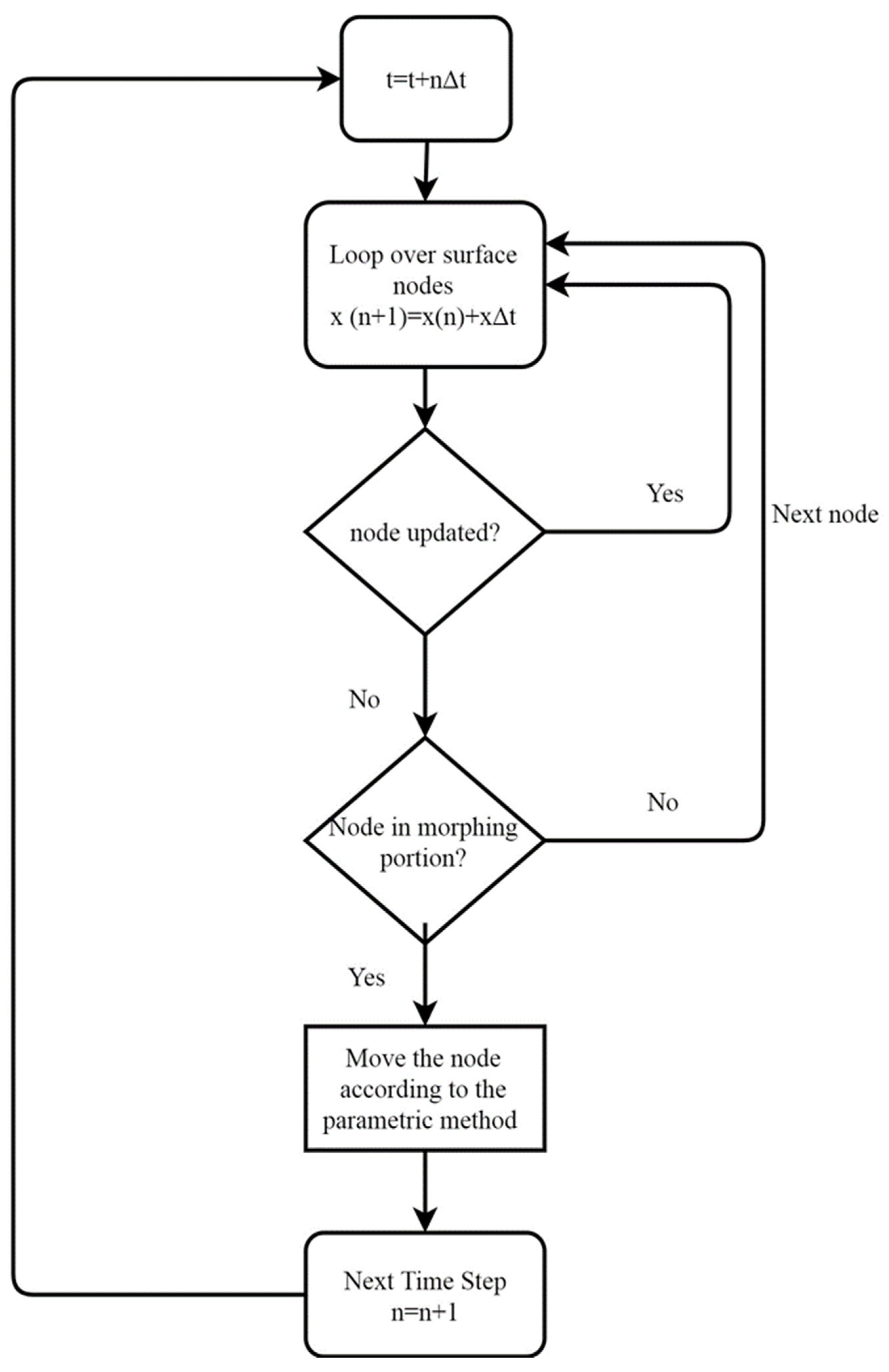
To drive the dynamic meshing schemes in ANSYS Fluent, a UDF was developed to incorporate the unsteady parametrization method explained in Section 2.2. The UDF makes use of the DEFINE_GRID_MOTION macro embedded in Fluent, and follows the algorithm illustrated by the flowchart in Figure 1. The source code of the UDF was realised as an open source [58].
3. Numerical Procedure
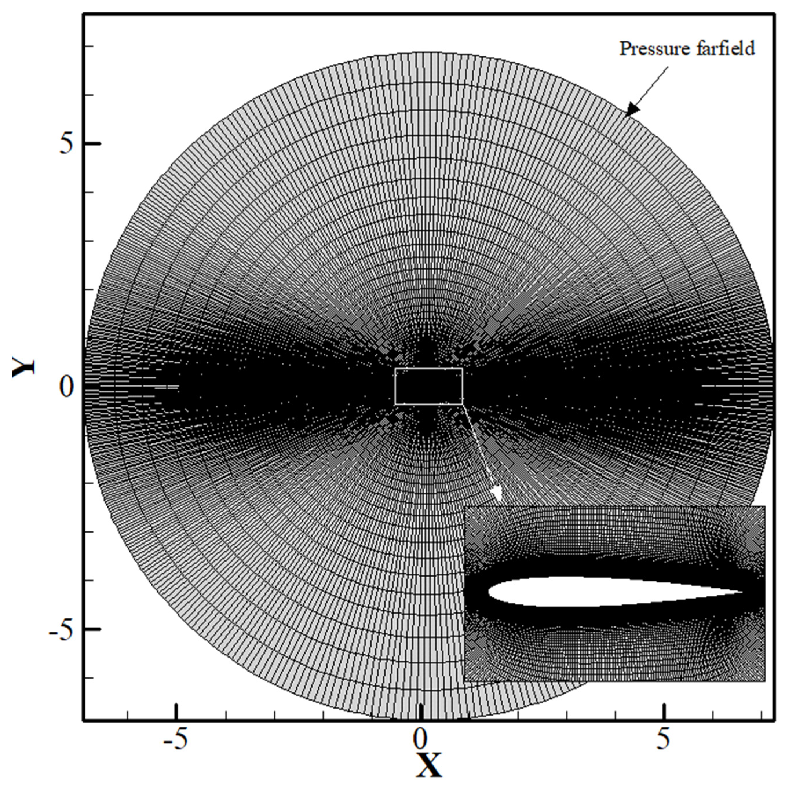
The flow domain consists of a NACA 0012 airfoil with a sharp TE, the pressure far-field was placed at least 30 chord lengths (c) from the TE, and a structured O-grid type mesh (Figure 2) was generated around the airfoil. Three sets of meshes were generated to determine mesh independency. The sizes of the grids were 60k, 100k and 400k cells for the coarse, medium and fine grids, respectively. The number of points on the surface of the airfoil ranged from 600 to 1600 points for the fine mesh. The distribution of points on the airfoil was achieved using a hyperbolic function with points clustered near the LE and TE (spacing of 10−4 m) in order to capture fine geometric features. The inflation layer was refined to achieve a y+ between 0.5 and 1 for the first layer on the wall. A cell height of 8 × 10⁻⁶ m was chosen in order to satisfy such requirement, with a growth rate of 1.1 away from the wall. The grids were created in an iterative process to be suitable for the acoustics application, therefore over 90% of the grids created have a CFL number less than one, in which all grids in the near field regions around the airfoil have a CFL less than one. This choice is deemed sufficient for the present tonal noise investigation [59].
The Fractional Step Method (FSM) of the Non-Iterative Time-Advancement scheme (NITA) [37,60] was used as it results in significant computational savings [59]. A second order upwind discretization scheme was used for pressure, density and diffusion quantities and the least-squares cell based spatial discretization for the gradients. For the momentum terms, a central differencing scheme was used to limit the numerical dissipation to capture smaller vortex structures relevant for the acoustics analysis. Given the low Mach number of 0.115, the flow was thus assumed incompressible for all the cases studied in this work. As the farfield boundary condition was used, one of the requirements of ANSYS Fluent is to use the ideal gas law for the density and therefore solving the energy equation as well to meet such requirement.
A second order transient formulation was used for all the simulations. A time step of Δt = 10−5 s was employed in the simulation, it was found that most of the cells in the important flow regions had a CFL number smaller than unity, which guarantees the stability of the NITA scheme and follows best practices scale resolving simulations (SRS) [59]. Diffusion-based smoothing was applied for all the simulation cases, with a boundary-distance parameter equal to 1.5 for a greater preservation of the near-wall mesh.
The FW-H acoustic analogy was used for the far-field noise prediction. The acoustics data was acquired in all simulations for at least 20,000 time steps after a minimum of two flow-through times. In order to re-create the same setup as Brooks et al. [36], the acoustic receiver was placed perpendicular to the airfoil TE at about 1.22 m away in all cases. Finally, as explained in Section 2.1.3, the two-dimensional FW-H acoustic analogy implemented in Fluent needs a source correlation length as an input parameter to account for the spanwise effect of the 2D airfoil in order to evaluate the integrals [37]. This length is problem-dependent and usually can be obtained from empirical correlations or numerical experimentation [48,52,53]. Numerical experimentations for the present case showed that a correlation length in the vicinity of 0.5c produced the closest SPL levels for the main tones compared with Brooks’ experiment [36], this value is consistent with other studies performed using a similar Reynolds number and characteristic length (e.g., chord) [27]. Therefore, this correlation length was used throughout the study.
4. Results and Discussion
4.1. Verification and Validation
Results from the previously mentioned cases are presented in the following. First, the 2D predictions of the unmorphed NACA 0012 are compared with Brooks’ experiment and published 2D RANS results at Re = 0.62 × 10⁶ [35]. This setup will be the one used later for the morphing case study. Section 4.1.2 presents the results of a comparative study between the 2D SBES results and 3D LES results obtained by Wolf et al. [35] of the same setup as Brooks’ experiment but at a slightly lower Re = 0.408 × 10⁶ (see, e.g., Table 1).
4.1.1. Unmorphed Case: M = 0.115, AoA = 4°, Re = 0.62 × 10⁶
To establish mesh independency of the obtained results, three sets of meshes were investigated, and the difference in lift and drag coefficients was monitored. Results showed that the difference in lift coefficient between the fine and coarse meshes was less than 1%.
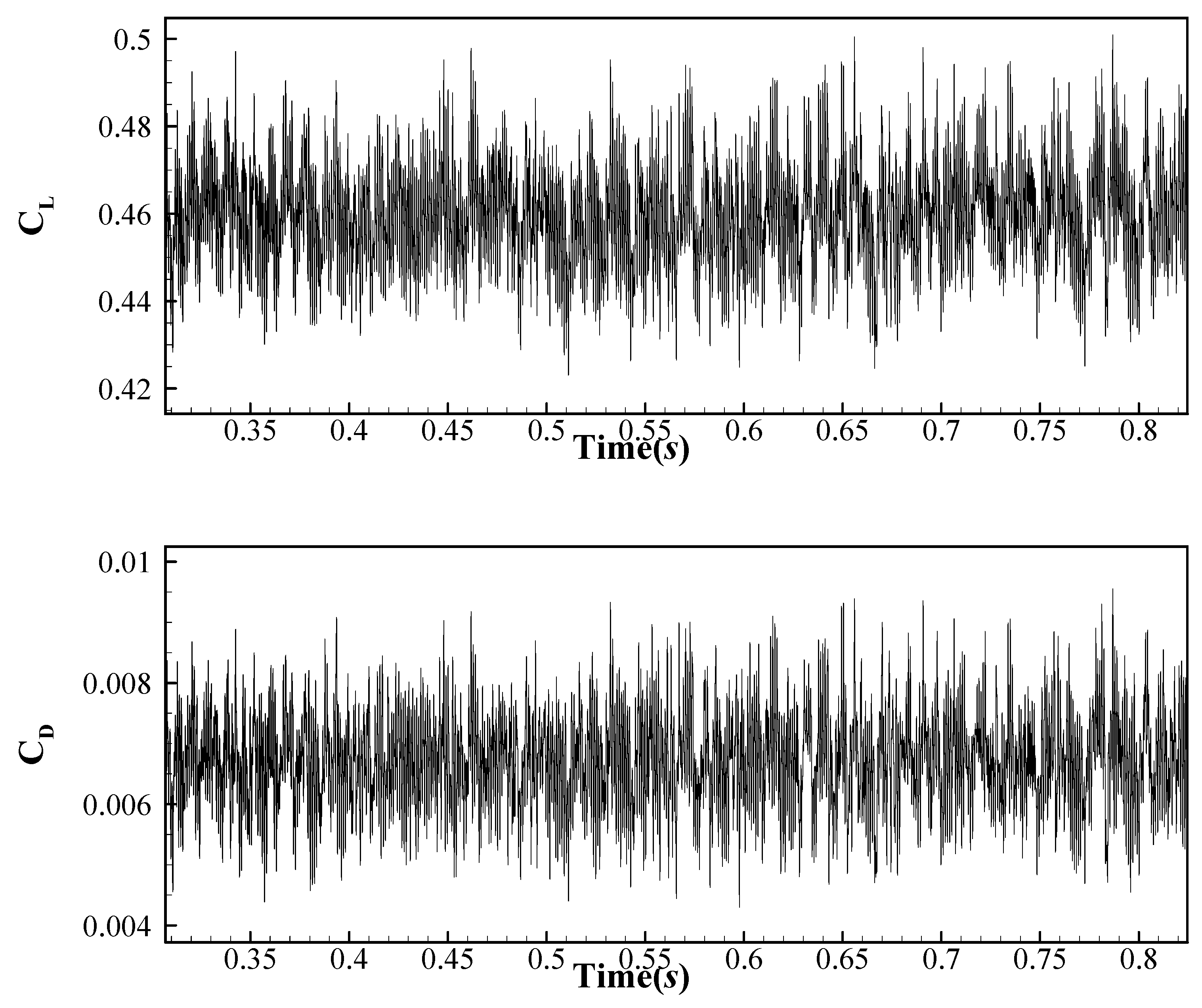
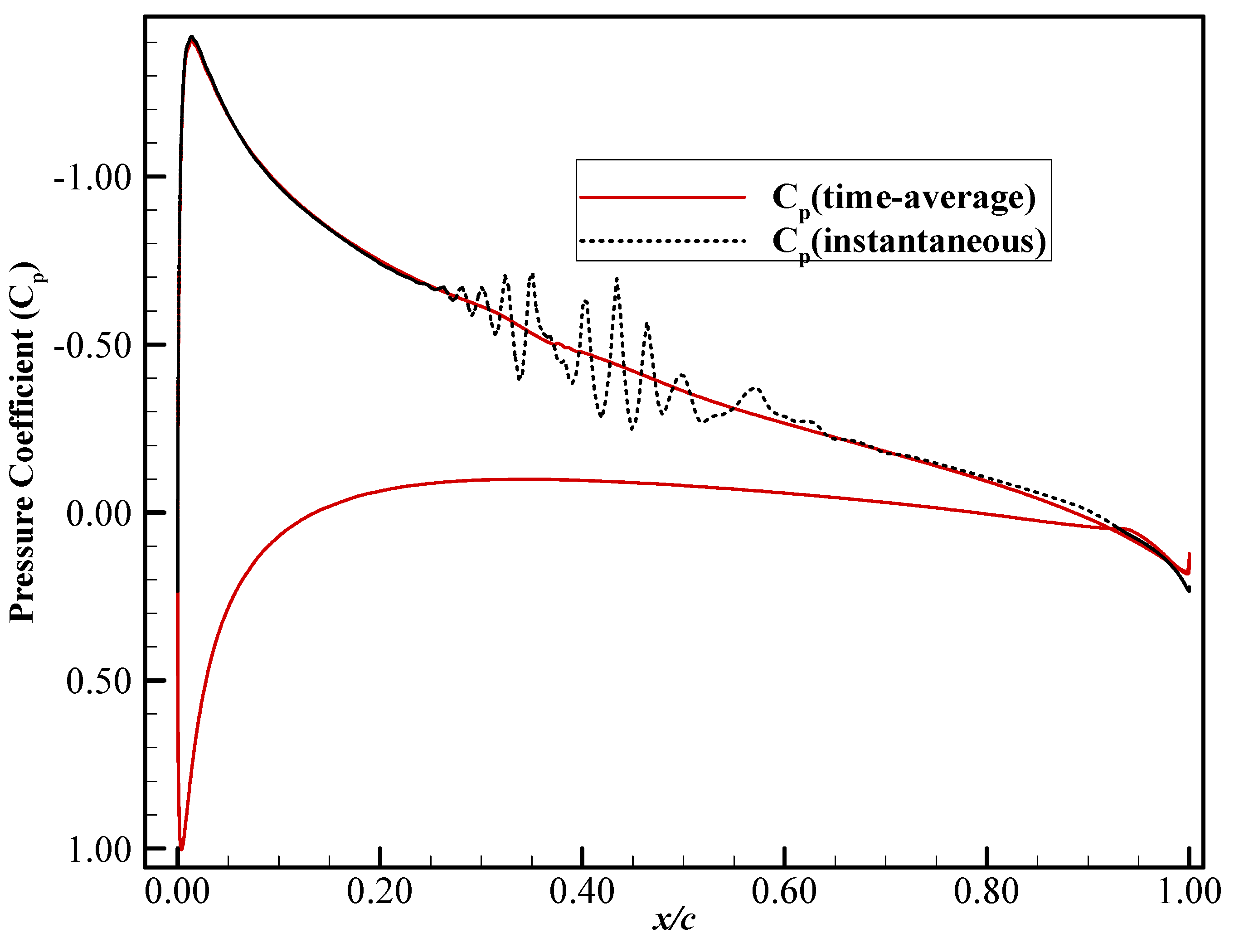
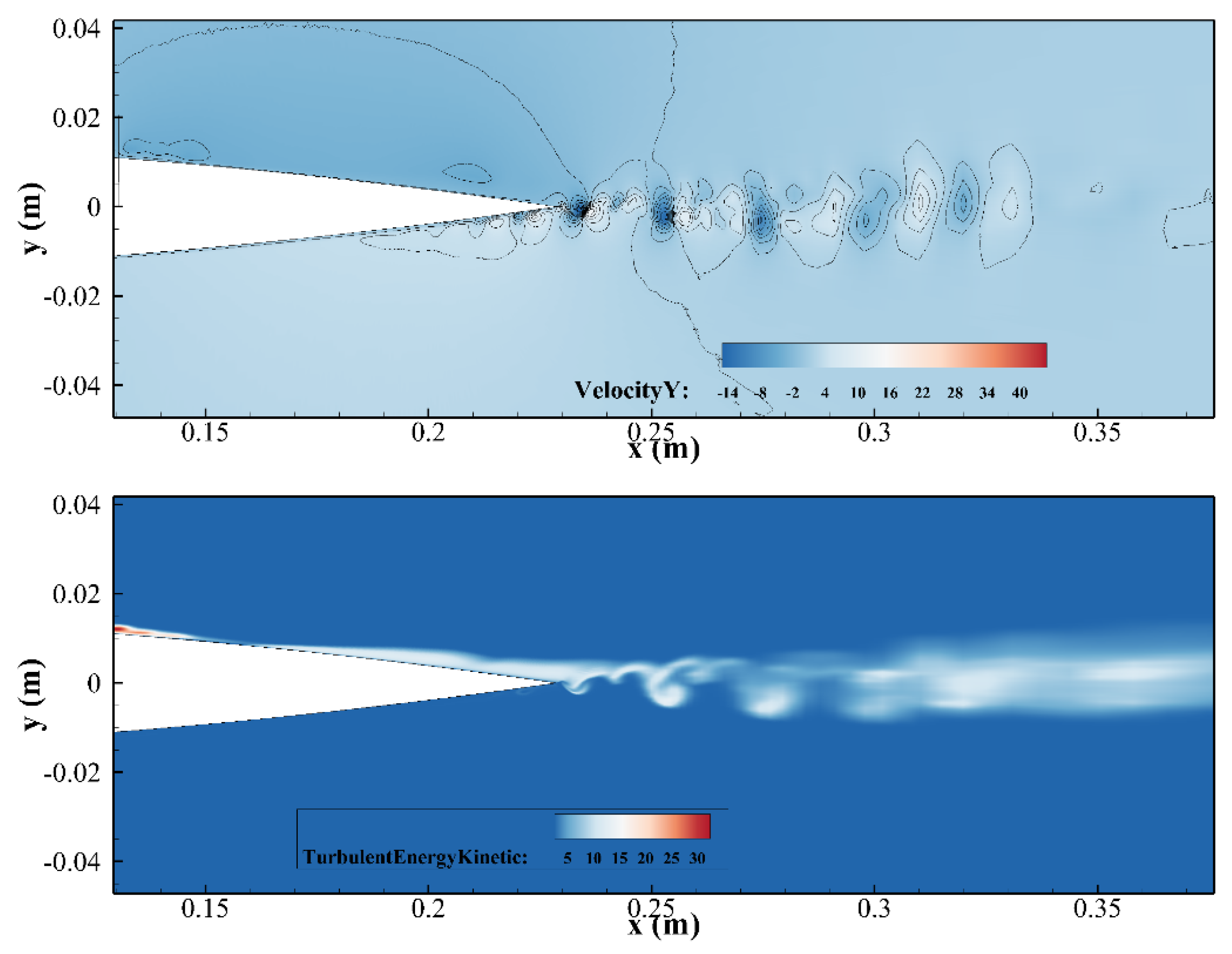
Figure 3 presents the instantaneous lift and drag coefficients data, the mean (time-averaged) values are compared with published numerical results from an unsteady RANS study by De Gennaro et al. [46] and with experimental results for a Reynolds number of 0.7 × 10⁶ of Sheldahl and Klimas [61]. Table 2 summarizes the time-averaged aerodynamic coefficients compared with published data. The lift coefficients for all studies compare well. For the drag coefficient, the SBES and URANS results have shown a 5.33% difference. Compared with the experimental study, both SBES and URANS under-predict the drag by 9.63% and 12.34%, respectively. The presence of the LBL instabilities is confirmed by various fluctuations presented on the suction side of the instantaneous pressure coefficient plot (see Figure 4). Later, LBL instabilities move downstream to interact with the laminar separation bubble presented near the TE on the pressure side.
This interaction gives rise to an acoustic source located in the near wake similar to what was proposed by Nash et al. [62]. Such interaction mechanism can be observed clearly in both vertical velocity and the Turbulent Kinetic Energy (TKE) contours (Figure 5).
Figure 6 shows the SPL in one-third octave band (SPL1/3) obtained using FW-H analogy for the three sets of grids studied, compared with experimental results from Brooks et al. [36] and URANS results of De Gennaro et al. [46] for the same configuration. The three sets of grids were able to show very similar behaviour when it comes to predicting the location and amplitude of the main tones and higher harmonics. The most prominent difference could be observed at higher frequencies, as the coarse mesh seems to over-predict the SPL compared with both the fine mesh and the experimental results.
Overall, the 2D FW-H simulation was able to accurately replicate the main tone location (~1.6 kHz) and SPL (75 dB observed in the experiment), which is in accordance with the tonal structure expected from literature [63,64]. Results obtained using SBES gave a slightly more accurate sound level at the main tone compared with the URANS study. For the off-tone regions, both URANS and SBES cannot predict the broadband part of the spectrum, due to the turbulent boundary layer–TE (TBL–TE) noise generation mechanism being highly three dimensional. This may explain the differences observed in the broadband spectra. A clear difference between the URANS and SBES can be seen at the higher harmonic location (~3.2 kHz), for which the URANS under-predicts the sound level whereas the SBES over-predicts it.
The SBES over-prediction might originate from the LES region of the flow, since the pressure fluctuations do not dissipate in the spanwise direction causing an over-prediction especially in high frequency regions (corresponding to small turbulence eddies). A similar over-prediction was observed in previous 2D studies ([48,52,65]). Finally, De Gennaro et al. [46] showed that the weight of the broadband component is negligible in the third octave band which might explain why the SPL of the main peak is not affected.
4.1.2. Unmorphed 2D vs. 3D case: M = 0.115, AoA = 5°, Re = 0.408 × 10⁶
This section presents the results of a comparative study performed for the purpose of gaining an additional understanding of possible differences between 2D and 3D predictions. Given the prohibitive computational cost of performing a 3D scale resolving simulation, the study conducted by Wolf et al. [35] was replicated using 2D simulations. Wolf et al. [35] performed a 3D simulation of Brooks’ experiment using a compressible LES approach that required over 45 Million mesh cells. For the 2D simulation, the same setup of the validation simulation was used, whilst ensuring to adjust the chord length in order to match the Reynolds number as in Wolf’s work.
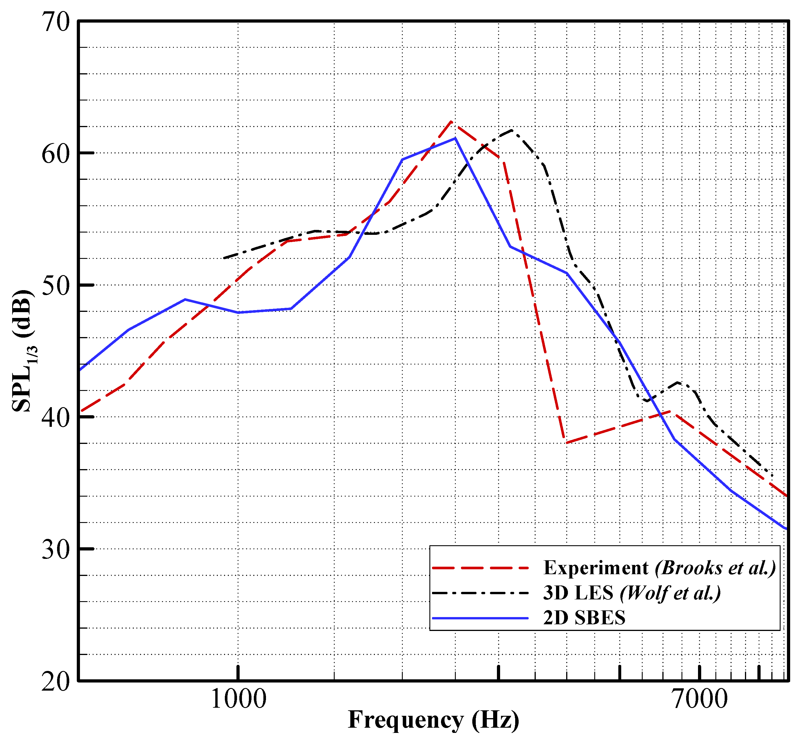
Figure 7 shows the SPL in one-third octave band (SPL1/3) obtained using 2D SBES and the FW-H analogy compared with both experimental results [35] and the 3D LES results [35]. The overall agreement between the 2D predictions and the experiment is satisfactory; the 2D simulation was able to correctly predict the location and SPL of the main tonal peak at 2.5 kHz, despite of a difference of 2 dB in SPL compared with the experiment. As expected, the broadband region shows a distinct discrepancy compared with the experiment. On the other hand, 3D LES results seem to predict well the broadband noise, yet a shift in the main tone peak location is observed in the 3D LES predictions (at ≈ 3kHz). This difference between the 3D LES and experiment could be explained by the tripping method employed in LES (suction and blowing near the LE) which was different from the experiment (trip wire near the LE).
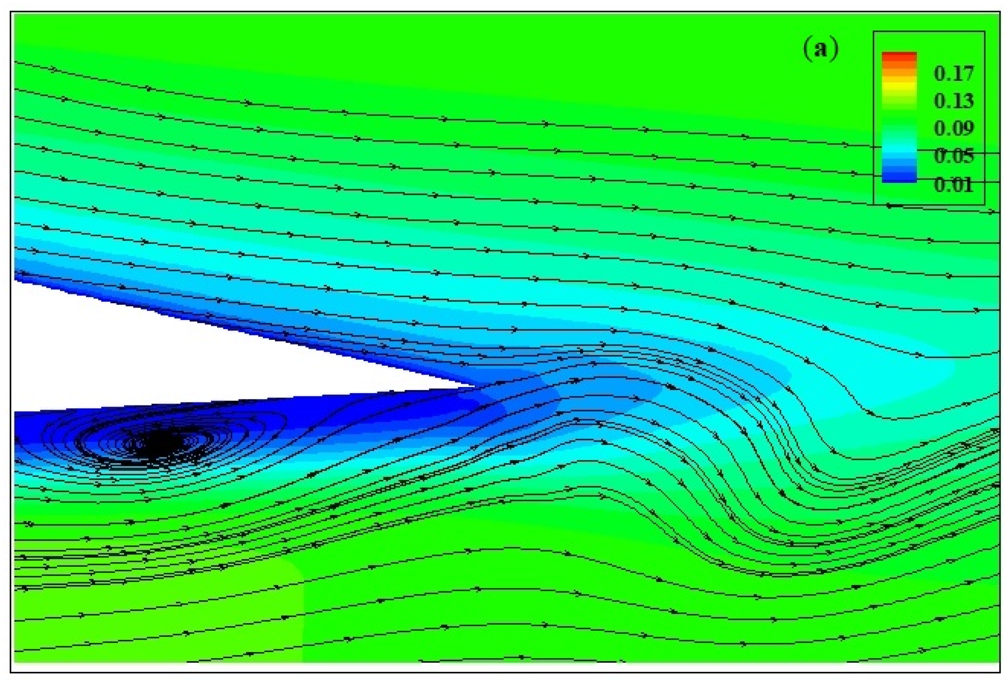
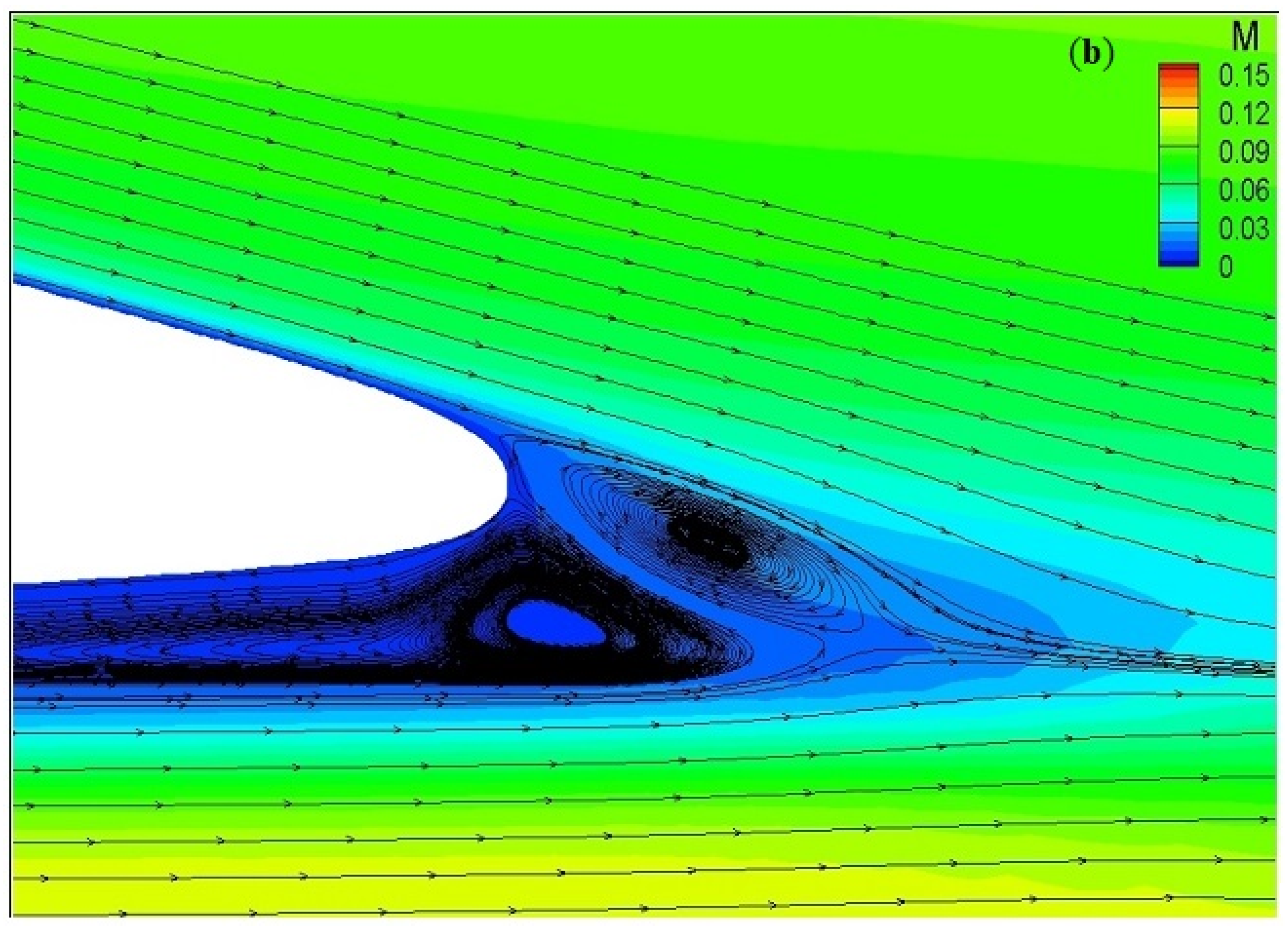
Figure 8 shows a comparison between the time-average Cp obtained using the 3D LES simulations of Wolf et al. [35] and the one obtained by the current 2D SBES model. An overall agreement is observed between the two. However, the effect that the tripping has on the suction side is clear in the 3D LES results, this tripping mechanism affecting the boundary layer thickness could be the origin in the shift observed. Another variance in the 3D LES result is the use of a rounded TE instead of a sharp TE like in the experiment. The rounded TE maybe inducing recirculation areas around the TE region which would affect the TE tonal noise being generated, thereby contributing to the difference obtained by Wolf et al. [35] in the tonal peak location. This is illustrated in Figure 9 where a side-by-side comparison of the time-averaged Mach number is presented showing the differences in TE geometry and flow behaviour between the two cases.
4.2. Harmonically Morphing Trailing Edge Flap
Having established the validity of the current 2D approach in correctly predicting tonal noise, this section presents a further aeroacoustic study of a NACA 0012 fitted with a harmonically morphing TEF to provide a practical example using the developed framework. The effects of harmonic morphing on the tonal noise are discussed afterwards.
Two case studies are considered: in the first case, the morphing frequency f was fixed at 100 Hz and two maximum deflection values were studied: wte = ± 0.01% c and wte = ± 0.1% c. These deflection and frequency values were inspired by similar published tests [23,24]. In the second case, the frequency was modified to f = 800 Hz at wte = ±0.01% c to compare it with the 100 Hz case and observe possible effects of changing the frequency for a fixed amplitude. All the numerical settings used are the same as the Re = 0.62 × 10⁶ unmorphed validation case; a statistically converged baseline NACA 0012 solution was obtained before engaging the dynamic meshing tool and starting the harmonic morphing after two through-flow time (0.4 s).
Throughout the harmonic morphing cycles, the grid was preserved at high quality; the TEF deformation had no major impact on the average values of the orthogonal quality and the cell equiangle skewness, the impact on the maximum values of these quantities was also negligible (0.04% difference). A diffusion parameter of 1.5 was used which enabled the deformation to diffuse well in the far-field, keeping the mesh near the wall intact and thus guaranteeing a good resolution of the near-wall flow.
The time-averaged aerodynamic coefficients for the fixed 100 Hz case are practically unchanged at both amplitudes as only a 0.3% difference in CL and CD was obtained compared with the unmorphed baseline results. On the other hand, when the TEF is harmonically morphed at f = 800 Hz, the average lift coefficient increased by about 0.7% while the drag coefficient decreased by 1.5%, giving an effective increase in the aerodynamic efficiency (CL/CD) of about 3%. This confirms that in addition to effects on tonal noise reduction, the harmonic morphing of the TEF could also result in some aerodynamic benefits for particular combinations of frequency and amplitude. Jodin et al. [23] observed similar effects and demonstrated that a reduction in large-scale instabilities and the breakdown of the LCSs due to a morphing flap contributed to a 5% decrease in drag.
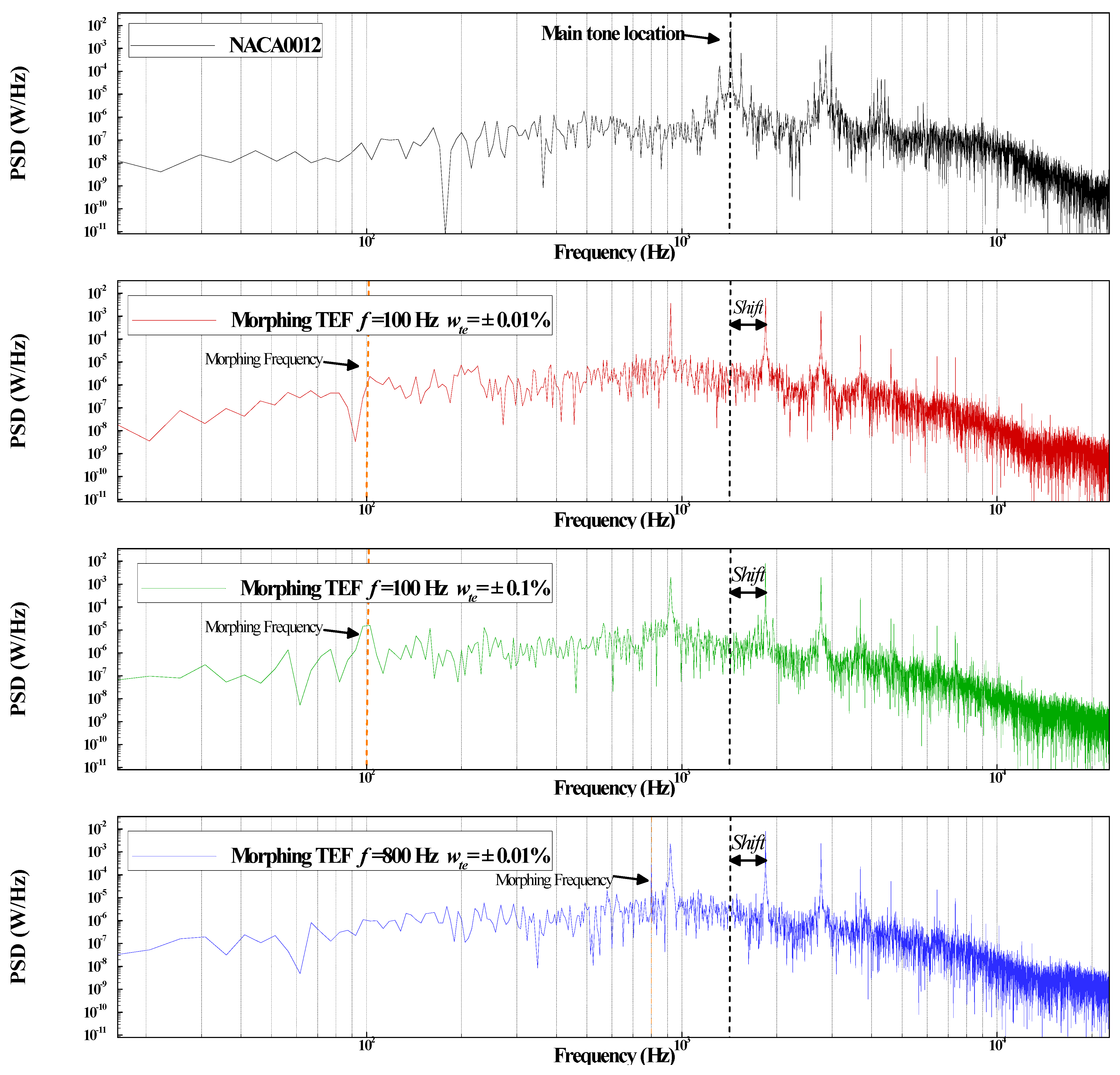
Figure 10 illustrates the acoustic pressure data collected at the receiver location for the cases studied. The pressure fluctuations appear to have similar amplitudes for all cases. A deeper comprehension can be gained from Figure 11 where the Power Spectral Density (PSD) plots obtained for the morphing configurations compared with the baseline NACA 0012 are presented. The main observation that can be drawn from the morphing cases and the baseline comparison is that the main tone location associated with LBL-VS tonal noise is shifted to a higher frequency, i.e., from 1.6 kHz to about 2 kHz. In addition, sub-harmonics are captured clearly with higher PSD levels for the morphing cases at location 900 Hz which was not captured for the baseline study.
When changing the morphing amplitudes from 0.01% to 0.1%, the peak associated with the morphing actuation frequency increases in PSD. The increase is proportional to the increase in morphing amplitude possibly due to larger amplitudes inducing large flow motions in the near-wake. This indicates that the morphing amplitudes could cause an increase in noise that is related to the physical oscillation.
Increasing the morphing frequency from 100 Hz to 800 Hz does not appear to have significant effect on the broadband region of the spectra. However, a sharp tonal peak is observed at the morphing frequency location, which indicates that the amplitude of 0.01% of the chord is possibly too small to cause any significant flow changes in the wake.
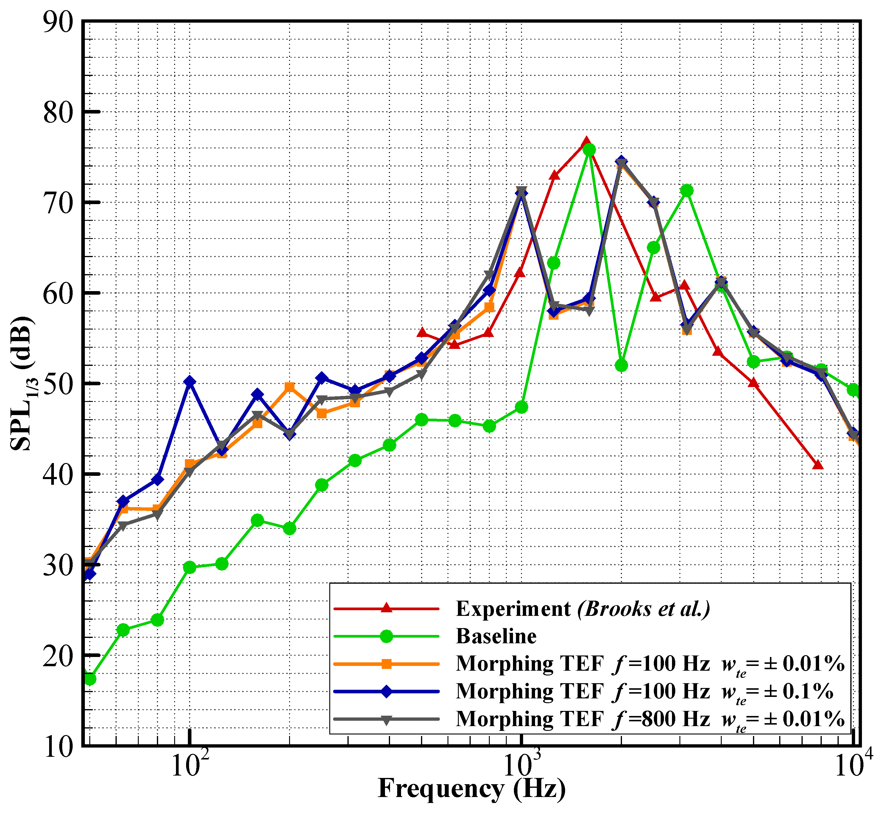
Figure 12 shows the SPL in one-third octave band comparing the baseline and the morphing cases, confirming results presented in the spectral analysis of Figure 7. The effect of the 100 Hz morphing frequency on the spectra is similar between the two amplitudes with the exception of a clear difference in the SPL levels near the 100 Hz location where the case with 0.1% amplitude seems to have a 9 dB higher SPL. The shift in the peak associated with the LBL-VS is clearly observed in the one third band plot, and a 1.5 dB noise reduction is associated with it. Possible explanations of these phenomena are discussed in the next section. Finally, the first superharmonic located at about 4 kHz experienced a significant 10 dB reduction, compared with the first superharmonic captured in the baseline airfoil case.
Effect of Harmonic Morphing
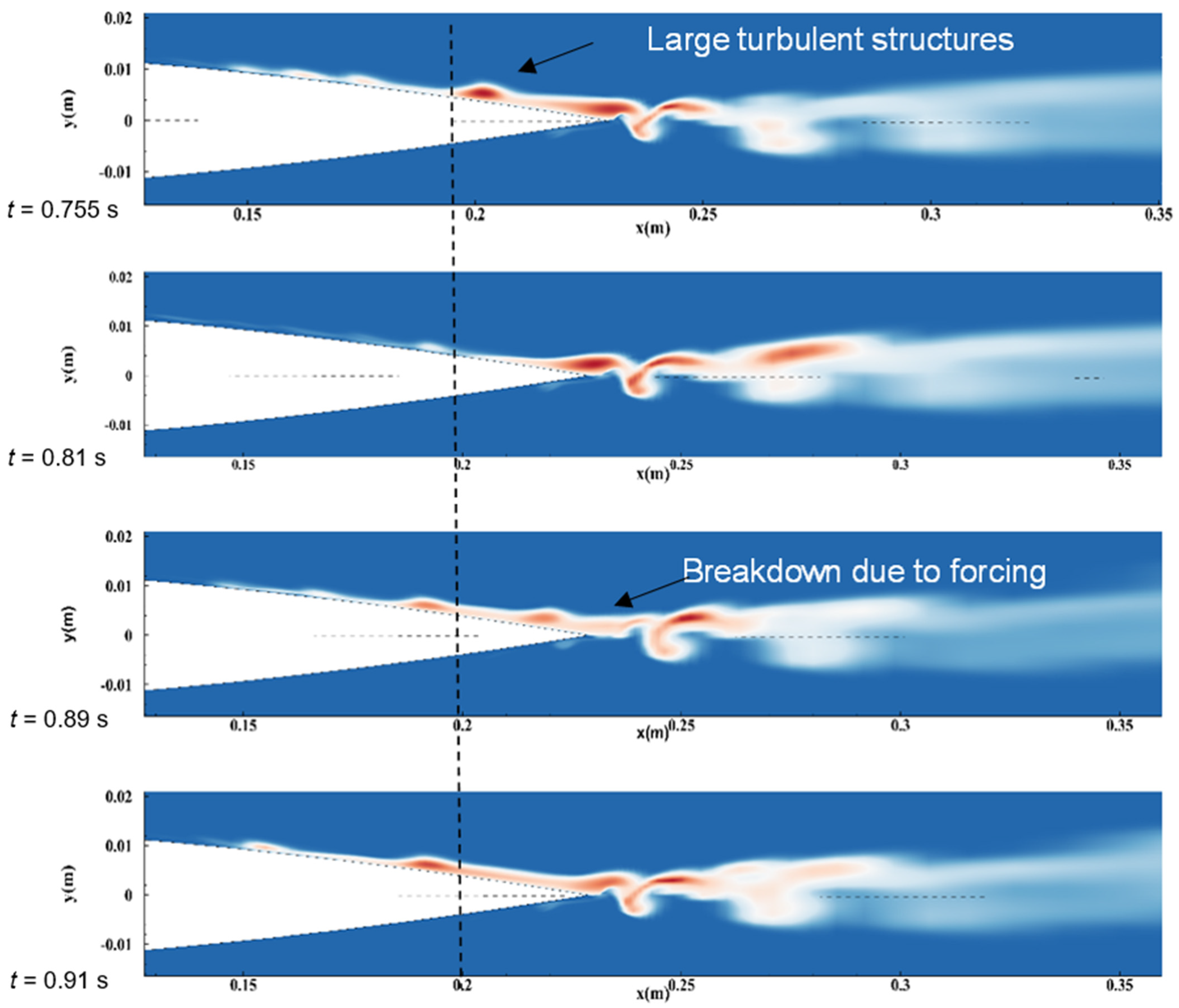
The underlying mechanism causing the observed shift in the tonal peak, the SPL reduction and the increase in the aerodynamic efficiency is still not yet clear from the current numerical studies. The decrease in drag indicates a change in the wake structure induced by the harmonic motion, which would possibly introduce a change towards higher frequency turbulence structures causing larger flow structures to break down at the TE, (see Figure 13). Similar effects on the drag were observed by Munday et al. [66] when using active forcing to alter the wake structure. It was found that under certain conditions, the actuations reduce the drag and yield a more streamlined wake structure by elongating it. This occurred when the forcing frequency was chosen to be close to the natural shedding frequency, resulting in a lock-on effect. Nevertheless, the same study by Munday et al. [66] observed instances where the actuation made the wake less streamlined and shortened, which increased the drag. Additionally, similar phenomena of breakdown due to forcing was observed in high fidelity studies of vibrating [18,24] where the breakdown led to a significant decrease in recirculation region on the upper side of the airfoil. However, the aforementioned studies did not provide extra insight into the effect of the acoustic spectra.
In the current study, the range of frequencies tested were all lower than the natural shedding frequency which means that even if a lock-on took place, it was a lock-on with one of the subharmonics which would explain the observed behaviour. Additionally, it appears that harmonic morphing for all the cases seems to alter the spectra regardless of the morphing frequency used, the only changes between predicted tonal frequencies observed are at the low frequency band for the 100 Hz morphing frequency. In this case, the effect of the amplitude seems to be predominant where the peak for the 0.1% case is higher compared with the 0.01% case. One possible explanation is that specific morphing amplitude and frequency couples interact differently with subharmonics producing different responses. In order to acquire a fundamental understanding of this harmonic morphing mechanism and exploit it as an efficient active flow control method for both aerodynamic and aeroacoustic enhancement, it is necessary to study a range of forcing frequencies in both the lock-on and non-lock-on regions. Of course, to do an in-depth analysis of the turbulence structures would require higher-fidelity 3D LES or even direct numerical simulation (DNS), but this is beyond the scope of the present study.
5. Conclusions and Future Work
In this paper, a framework to perform aeroacoustic studies of a harmonically morphing TEF is introduced. It is based on a modified unsteady parametrization method defining the TEF motion, and dynamic meshing tools for mesh deformation. This framework can be generally applied to 2D and 3D problems; however, given the prohibitive computational cost of 3D simulations and the large number of possible parameters to consider, the present study is restricted to 2D harmonic deformations and their effects on tonal noise.
A hybrid turbulence model, SBES, was used and its performance was coupled with the Ffowcs-Williams and Hawkings (FW-H) acoustic analogy benchmarked for 2D cases. A 2D aeroacoustic study of an unmorphed NACA 0012 airfoil was performed using the developed framework. Results compare well with published numerical and experimental data. It was found that the SBES model was able to accurately predict the location and amplitude of the main tone frequency related to the laminar boundary-layer instabilities. The structure of the main tone captured is also in good agreement with the published literature. In addition, a comparative study between 2D SBES predictions and published 3D LES results was conducted. It was found that the 2D simulations capture the tonal noise given its pseudo 2D generation mechanisms well.
The use of a hybrid RANS-LES model in the present 2D study showed to be useful for the purpose of demonstrating trends and for providing some guidance for future quasi- or full-3D simulations, especially given the exorbitant computational cost a 3D simulation coupled with dynamic mesh. For an exploratory study such as the current one, the hybrid RANS-LES offered a balanced approach between accuracy and computational requirements and an accurate prediction of tonal noises.
Results for three morphing configurations were presented. Two morphing amplitudes of 0.01% and 0.1% were at a fixed frequency (f = 100 Hz); then, the amplitude was fixed at 0.01% and two frequencies were studied (100 Hz and 800 Hz). It was found that up to a 3% increase in aerodynamic efficiency was possible using the 800 Hz frequency, whereas the 100 Hz frequency had negligible impact on the aerodynamic efficiency.
In terms of aeroacoustic effects, the morphing TEF appears to shift the main tone to a higher frequency (from 1.6 to 2 kHz) with a noise reduction of 1.5 dB for the main tone and up to 10 dB for the first superharmonic. The underlying mechanism causing these effects is still unclear but a possible lock-on with a subharmonic could be the cause for the change in the wake structure producing the observed frequency shift and drag reduction.
For future work, it will be necessary to test a wider range of morphing frequency/amplitude pairs in order to explore optimal configurations that could enhance the aerodynamic performance further while keeping the same noise level if not reducing it. Likewise, exploring the use of the harmonic morphing at higher angles of attack is imperative given the higher impact expected and the practical application possible.
Finally, to capture a more realistic depiction of the physical phenomena, especially within large flow separation regions, the problem needs to be analysed in 3D using LES or even Direct Numerical Simulation (DNS). Such formulations will be able to resolve the small turbulence structures which would offer a better understanding of the effects causing the shift and noise reductions observed, particularly the broadband noise.
Author Contributions
Conceptualization, C.A., A.B. and Y.Y.; methodology, C.A., A.B. and Y.Y.; software, C.A.; validation, C.A., A.B. and Y.Y.; formal analysis, C.A., A.B. and Y.Y.; investigation, C.A., A.B. and Y.Y.; resources, C.A., A.B. and Y.Y.; data curation, C.A.; writing—original draft preparation, C.A., A.B. and Y.Y.; writing—review and editing, C.A., A.B. and Y.Y.; visualization, C.A.; supervision, A.B. and Y.Y.; project administration, A.B. and Y.Y.; funding acquisition, Y.Y. All authors have read and agreed to the published version of the manuscript.
Funding
This research received no external funding.
Institutional Review Board Statement
Not applicable.
Informed Consent Statement
Not applicable.
Data Availability Statement
The data presented in this study are available on request from the corresponding author.
Acknowledgments
The first author gratefully acknowledges the studentship funding received from the Engineering Modelling and Simulation Research Group, University of the West of England, Bristol, UK.
Conflicts of Interest
The authors declare no conflict of interest.
References
- European Commission; Dareki, M.; Edelstenne, C.; Enders, T.; Fernandez, E.; Hartman, P.; Herteman, J.-P.; Kerkloh, M.; King, I.; Ky, P.; et al. Flightpath 2050: Europe’s Vision for Aviation. European Commission: Brussels, Belgium, 2011; 24p, ISBN 978-92-79-19724-6. [Google Scholar] [CrossRef]
- Nguyen, N. Project Elastically Shaped Future Air Vehicle Concept; NASA Innovation Fund Award: Washington, DC, USA, 2010.
- Macaraeg, M. Fundamental investigations of airframe noise. In Proceedings of the 4th AIAA/CEAS Aeroacoustics Conference, Toulouse, France, 2–4 June 1998; American Institute of Aeronautics and Astronautics: Toulouse, France, 1998; pp. 123–132. [Google Scholar] [CrossRef] [Green Version]
- Abdessemed, C.; Yao, Y.; Bouferrouk, A.; Narayan, P. Analysis of a 3D Unsteady Morphing Wing with Seamless Side-edge Transition. In Proceedings of the 36th AIAA Applied Aerodynamics Conference, Atlanta, GA, USA, 25–29 June 2018; AIAA: Atlanta, GA, USA, 2018; p. 2897416. [Google Scholar] [CrossRef] [Green Version]
- Kota, S.; Flick, P.; Collier, F.S. Flight Testing of FlexFloilTM Adaptive Compliant Trailing Edge. In Proceedings of the 54th AIAA Aerospace Sciences Meeting, San Diego, CA, USA, 4–8 January 2016; pp. 1–13. [Google Scholar] [CrossRef]
- NASA Hear This: 30 Percent Less Noise. Available online: https://www.nasa.gov/centers/armstrong/feature/ACTE_30_percent_less_noise.html (accessed on 8 October 2018).
- Fincham, J.H.S.; Friswell, M.I. Aerodynamic optimisation of a camber morphing aerofoil. Aerosp. Sci. Technol. 2015, 43, 245–255. [Google Scholar] [CrossRef] [Green Version]
- Afonso, F.; Vale, J.; Lau, F.; Suleman, A. Performance based multidisciplinary design optimization of morphing aircraft. Aerosp. Sci. Technol. 2017, 67, 1–12. [Google Scholar] [CrossRef]
- Greenblatt, D.; Wygnanski, I.J. Control of flow separation by periodic excitation. Prog. Aerosp. Sci. 2000, 36, 487–545. [Google Scholar] [CrossRef]
- Winant, C.D.; Browand, F.K. Vortex pairing: The mechanism of turbulent mixing-layer growth at moderate Reynolds number. J. Fluid Mech. 1974, 63, 237. [Google Scholar] [CrossRef]
- Cattafesta, L.N.; Sheplak, M. Actuators for Active Flow Control. Annu. Rev. Fluid Mech. 2011, 43, 247–272. [Google Scholar] [CrossRef] [Green Version]
- Huang, L.; Huang, P.G.; LeBeau, R.P.; Hauser, T. Numerical Study of Blowing and Suction Control Mechanism on NACA0012 Airfoil. J. Aircr. 2004, 41, 1005–1013. [Google Scholar] [CrossRef]
- Hue, D.; François, C.; Dandois, J.; Gebhardt, A. Simulations of an aircraft with constant and pulsed blowing flow control at the engine/wing junction. Aerosp. Sci. Technol. 2017, 69, 659–673. [Google Scholar] [CrossRef] [Green Version]
- Kim, H.; Liou, M. Flow simulation and drag decomposition study of N3-X hybrid wing-body configuration. Aerosp. Sci. Technol. 2019, 85, 24–39. [Google Scholar] [CrossRef]
- Jukes, T.N.; Choi, K.-S. Flow control around a circular cylinder using pulsed dielectric barrier discharge surface plasma. Phys. Fluids 2009, 21, 084103. [Google Scholar] [CrossRef]
- Ebrahimi, A.; Hajipour, M. Flow separation control over an airfoil using dual excitation of DBD plasma actuators. Aerosp. Sci. Technol. 2018, 79, 658–668. [Google Scholar] [CrossRef]
- Krzysiak, A.; Narkiewicz, J. Aerodynamic Loads on Airfoil with Trailing-Edge Flap Pitching with Different Frequencies. J. Aircr. 2006, 43, 407–418. [Google Scholar] [CrossRef]
- Jones, G.; Santer, M.; Debiasi, M.; Papadakis, G. Control of flow separation around an airfoil at low Reynolds numbers using periodic surface morphing. J. Fluids Struct. 2018, 76, 536–557. [Google Scholar] [CrossRef] [Green Version]
- Abdessemed, C.; Yao, Y.; Bouferrouk, A.; Narayan, P. Aerodynamic Analysis of a harmonically Morphing Flap Using a Hybrid Turbulence Model and Dynamic Meshing. In Proceedings of the 36th AIAA Applied Aerodynamics Conference, Atlanta, GA, USA, 25–29 June 2018; American Institute of Aeronautics and Astronautics: Reston, VA, USA, 2018; pp. 1–15. [Google Scholar] [CrossRef]
- Seifert, A.; Eliahu, S.; Greenblatt, D.; Wygnanski, I. Use of Piezoelectric Actuators for Airfoil Separation Control. AIAA J. 1998, 36, 1535–1537. [Google Scholar] [CrossRef]
- Kegerise, M.A.; Cabell, R.H.; Cattafesta, L.N. Real-time feedback control of flow-induced cavity tones-Part 1: Fixed-gain control. J. Sound Vib. 2007, 307, 906–923. [Google Scholar] [CrossRef]
- Liggett, N.; Smith, M.J. The physics of modeling unsteady flaps with gaps. J. Fluids Struct. 2013, 38, 255–272. [Google Scholar] [CrossRef]
- Scheller, J.; Chinaud, M.; Rouchon, J.F.; Duhayon, E.; Cazin, S.; Marchal, M.; Braza, M. Trailing-edge dynamics of a morphing NACA0012 aileron at high Reynolds number by high-speed PIV. J. Fluids Struct. 2015, 55, 42–51. [Google Scholar] [CrossRef] [Green Version]
- Jodin, G.; Motta, V.; Scheller, J.; Duhayon, E.; Döll, C.; Rouchon, J.F.; Braza, M. Dynamics of a hybrid morphing wing with active open loop vibrating trailing edge by time-resolved PIV and force measures. J. Fluids Struct. 2017, 74, 263–290. [Google Scholar] [CrossRef] [Green Version]
- Abdessemed, C.; Yao, Y.; Bouferrouk, A.; Narayan, P. Morphing airfoils unsteady flow analysis using dynamic meshing. Int. J. Numer. Methods Heat Fluid Flow 2017, 23. [Google Scholar] [CrossRef] [Green Version]
- Abdessemed, C.; Yao, Y.; Narayan, P.; Bouferrouk, A. Unsteady parametrization of a morphing wing design for improved aerodynamic performance. In Proceedings of the 52rd 3AF International Conference on Applied Aerodynamics, Lyon, France, 27–29 March 2017; pp. 1–10. [Google Scholar]
- Alqash, S.; Dhote, S.; Behdinan, K. Predicting far-field noise generated by a landing gear using multiple two-dimensional simulations. Appl. Sci. 2019, 9, 4485. [Google Scholar] [CrossRef] [Green Version]
- Doolan, C.J. Computational bluff body aerodynamic noise prediction using a statistical approach. Appl. Acoust. 2010, 71, 1194–1203. [Google Scholar] [CrossRef]
- Brentner, K.S.; Rumsey, C.L.; Cox, J.S.; Younis, B.A. Computation of Sound Generated By Flow Over A Circular Cylinder: An Acoustic Analogy Approach. In Proceedings of the NASA Conference Publication; NASA: Washington, DC, USA, 1996; pp. 1–7. [Google Scholar]
- Arunajatesan, S.; Sinha, N. Hybrid RANS-LES Modeling for Cavity Aeroacoutics Predictions. Int. J. Aeroacoust. 2003, 2, 65–93. [Google Scholar] [CrossRef]
- Housman, J.A.; Stich, G.D.; Kiris, C.C. Predictions of slat noise from the 30P30N at high angles of attack using zonal hybrid rans-les. In Proceedings of the 25th AIAA/CEAS Aeroacoustics Conference, Delft, The Netherlands, 20–23 May 2019; p. 2438. [Google Scholar] [CrossRef] [Green Version]
- Mahak, M.; Naqavi, I.Z.; Tucker, P.G. Cost-effective hybrid RANS-LES type method for jet turbulence and noise prediction. Int. J. Aeroacoust. 2017, 16, 97–111. [Google Scholar] [CrossRef]
- Syawitri, T.P.; Yao, Y.; Yao, J.; Chandra, B. Assessment of stress-blended eddy simulation model for accurate performance prediction of vertical axis wind turbine. Int. J. Numer. Methods Heat Fluid Flow 2020. [Google Scholar] [CrossRef]
- Pratomo, H.P.S.; Suprianto, F.D.; Sutrisno, T. Hybrid turbulence models: Recent progresses and further researches. In Proceedings of the 1st International Conference on Automotive, Manufacturing, and Mechanical Engineering, Bali, Indonesia, 26−28 September 2018; EDP Sciences: Les Ulis, France, 2019; Volume 130, p. 1013. [Google Scholar] [CrossRef]
- Wolf, W.R.; Lele, S.K. Trailing-Edge Noise Predictions Using Compressible Large-Eddy Simulation and Acoustic Analogy. AIAA J. 2012, 50, 2423–2434. [Google Scholar] [CrossRef]
- Brooks, T.F.; Pope, D.S.; Marcolini, M. Airfoil Self-Noise and Prediction; NASA Technical Report; 1989.
- ANSYS Release 18.2, Help System; ANSYS Inc.: Canonsburg, PA, USA, 2018.
- Menter, F. Stress-blended eddy simulation (SBES)—A new paradigm in hybrid RANS-LES modeling. In Notes on Numerical Fluid Mechanics and Multidisciplinary Design; Springer: Cham, Switzerland, 2016; Volume 137, pp. 27–37. ISBN 978-3-319-70031-1. [Google Scholar] [CrossRef]
- Nicoud, F.; Ducros, F. Subgrid-scale stress modelling based on the square of the velocity gradient tensor. Flow Turbul. Combust. 1999, 62, 183–200. [Google Scholar] [CrossRef]
- Weihing, P.; Letzgus, J.; Lutz, T.; Krämer, E. Development of alternative shielding functions for detached-eddy simulations. In Progress in Hybrid RANS-LES Modelling; Springer: Cham, Switzerland, 2020; pp. 109–118. [Google Scholar]
- Spalart, P.R.; Deck, S.; Shur, M.L.; Squires, K.D.; Strelets, M.K.; Travin, A. A new version of detached-eddy simulation, resistant to ambiguous grid densities. Theor. Comput. Fluid Dyn. 2006, 20, 181–195. [Google Scholar] [CrossRef]
- Williams, J.E.F.; Hawkings, D.L. Sound Generation by Turbulence and Surfaces in Arbitrary Motion. Philos. Trans. R. Soc. A Math. Phys. Eng. Sci. 1969, 264, 321–342. [Google Scholar] [CrossRef]
- Lighthill, M.J. On sound generated aerodynamically I. General theory. Proc. R. Soc. Lond. A R. Soc. 1952, 211, 564–587. [Google Scholar]
- Garipova, L.I.; Batrakov, A.S.; Kusyumov, A.N.; Mikhaylov, S.A.; Barakos, G. Aerodynamic and acoustic analysis of helicopter main rotor blade tips in hover. Int. J. Numer. Methods Heat Fluid Flow 2016, 26, 2101–2118. [Google Scholar] [CrossRef]
- Lockard, D.P. Efficient, two-dimensional implementation of the Ffowcs Williams and Hawkings equation. J. Sound Vib. 2000, 229, 897–911. [Google Scholar] [CrossRef]
- De Gennaro, M.; Kühnelt, H.; Zanon, A. Numerical Prediction of the Tonal Airborne Noise for a NACA 0012 Aerofoil at Moderate Reynolds Number Using a Transitional URANS Approach. Arch. Acoust. 2017, 42, 653–675. [Google Scholar] [CrossRef] [Green Version]
- Golubev, V.V.; Nguyen, L.; Mankbadi, R.R.; Roger, M.; Visbal, M.R. On Flow-Acoustic Resonant Interactions in Transitional Airfoils. Int. J. Aeroacoust. 2014, 13, 1–38. [Google Scholar] [CrossRef] [Green Version]
- Singer, B.A.; Lockard, D.P.; Brentner, K.S. Computational Aeroacoustic Analysis of Slat Trailing-Edge Flow. AIAA J. 2000, 38, 1558–1564. [Google Scholar] [CrossRef]
- Golubev, V.; Nguyen, L.; Roger, M.; Visbal, M. On Interaction of Airfoil Leading and Trailing Edge Noise Sources in Turbulent Flow. In Proceedings of the 17th AIAA/CEAS Aeroacoustics Conference (32nd AIAA Aeroacoustics Conference), Portland, OR, USA, 5–8 June 2011; American Institute of Aeronautics and Astronautics: Reston, VA, USA, 2011; p. 2859. [Google Scholar] [CrossRef]
- Golubev, V.; Nguyen, L.; Roger, M.; Visbal, M. High-Accuracy Simulations of Flow-Acoustic Resonant Interactions in Airfoil Transitional Boundary Layers. In Proceedings of the 18th AIAA/CEAS Aeroacoustics Conference (33rd AIAA Aeroacoustics Conference), Colorado Springs, CO, USA, 4–6 June 2012; American Institute of Aeronautics and Astronautics: Reston, VA, USA, 2012; pp. 4–6. [Google Scholar] [CrossRef]
- Golubev, V.V.; Nguyen, L.; Mankbadi, R.R.; Dudley, J.G.; Visbal, M.R. On Self-Sustained Flow-Acoustic Resonant Interactions in Airfoil Transitional Boundary Layers. In Proceedings of the 43rd Fluid Dynamics Conference, San Diego, CA, USA, 24–27 June 2013; American Institute of Aeronautics and Astronautics: Reston, VA, USA, 2013; pp. 1–16. [Google Scholar] [CrossRef]
- Kato, C.; Iida, A.; Takano, Y.; Fujita, H.; Ikegawa, M. Numerical prediction of aerodynamic noise radiated from low Mach number turbulent wake. In Proceedings of the 31st Aerospace Sciences Meeting, Reno, NV, USA, 11–14 January 1993; American Institute of Aeronautics and Astronautics: Reston, VA, USA, 1993. [Google Scholar] [CrossRef]
- Orselli, R.; Meneghini, J.; Saltara, F. Two and Three-Dimensional Simulation of Sound Generated by Flow Around a Circular Cylinder. In Proceedings of the 15th AIAA/CEAS Aeroacoustics Conference (30th AIAA Aeroacoustics Conference), Miami, FL, USA, 11–13 May 2009; American Institute of Aeronautics and Astronautics: Miami, FL, USA, 2009; p. 3270. [Google Scholar] [CrossRef] [Green Version]
- Seo, J.H.; Moon, Y.J. Aerodynamic noise prediction for long-span bodies. J. Sound Vib. 2007, 306, 564–579. [Google Scholar] [CrossRef]
- Bies, D.; Hansen, C. Engineering Noise Control: Theory and Practice; Taylor and Francis: New York, NY, USA, 2009; Volume 3, ISBN 9780203872406. [Google Scholar]
- Jacobs, E.; Ward, K.; Pinkerton, R. The characteristics of 78 related airfoil sections from tests in the variable-density wind tunnel. Natl. Advis. Comm. Aeronaut. 1933, 299–354. [Google Scholar] [CrossRef]
- Abdessemed, C. Dynamic Mesh Framework for Morphing Wings CFD. Ph.D. Thesis, University of the West of England, Bristol, UK, 2019. [Google Scholar]
- Abdessemed, C. Dynamic Mesh Framework for Morphing Wings CFD—User Defined Function; Zenodo: Genève, Switzerland, 2020. [Google Scholar] [CrossRef]
- Menter, F.R. Best Practice: Scale-Resolving Simulations in ANSYS CFD; ANSYS Inc.: Canonsburg, PA, USA, 2012; pp. 1–70. [Google Scholar] [CrossRef]
- Abdessemed, C.; Yao, Y.; Bouferrouk, A.; Narayan, P. Influence of non-iterative time-advancement schemes on the aerodynamic prediction of pitching airfoils using dynamic mesh. In Proceedings of the 8th International Symposium on Physics of Fluids (ISPF8), Xi’an, China, 10–13 June 2019. [Google Scholar]
- Sheldahl, R.E.; Klimas, P.C. Aerodynamic Characteristics of Seven Symmetrical Airfoil Sections through 180-Degree Angle of Attack for Use in Aerodynamic Analysis of Vertical Axis Wind Turbines; SAND-80-2114; Sandia National Laboratories: Albuquerque, NM, USA, 1981.
- Nash, E.C.; Lowson, M.V.; Mcalpine, A. Boundary-layer instability noise on aerofoils. J. Fluid Mech. 1999, 382. [Google Scholar] [CrossRef]
- Arbey, H.; Bataille, J. Noise generated by airfoil profiles placed in a uniform laminar flow. J. Fluid Mech. 1983, 134, 33–47. [Google Scholar] [CrossRef] [Green Version]
- Paterson, R.W.; Vogt, P.G.; Fink, M.R.; Munch, C.L. Vortex noise of isolated airfoils. J. Aircr. 1973, 10, 296–302. [Google Scholar] [CrossRef]
- Trümner, J.; Mundt, C. Comparison of Two Different CAA Methods for the Prediction of Far-Field Noise from Heated and Unheated Jets. In Proceedings of the 7th European Conference for Aeronautics and Aerospace Sciences, Milan, Italy, 3–6 July 2017; Volume 37, pp. 1–14. [Google Scholar]
- Munday, P.M.; Taira, K. On the lock-on of vortex shedding to oscillatory actuation around a circular cylinder. Phys. Fluids 2013, 25. [Google Scholar] [CrossRef]
Figure 1.
Algorithm used in the UDF to drive dynamic meshing in Fluent [37].
Figure 1.
Algorithm used in the UDF to drive dynamic meshing in Fluent [37].

Figure 2.
Details of the O-grid computational domain.

Figure 3.
Time history of lift (top) and drag (bottom) coefficients for unmorphed NACA 0012 at AoA = 4°.
Figure 3.
Time history of lift (top) and drag (bottom) coefficients for unmorphed NACA 0012 at AoA = 4°.

Figure 4.
Instantaneous and time-averaged pressure coefficient for unmorphed NACA 0012 at AoA = 4°, showing LBL instabilities on the suction side.
Figure 4.
Instantaneous and time-averaged pressure coefficient for unmorphed NACA 0012 at AoA = 4°, showing LBL instabilities on the suction side.

Figure 5.
Vertical velocity contours (Up) and TKE contours (Down) showing instability regions on the suction side near the TE of the unmorphed NACA 0012 airfoil.
Figure 5.
Vertical velocity contours (Up) and TKE contours (Down) showing instability regions on the suction side near the TE of the unmorphed NACA 0012 airfoil.

Figure 6.
SPL in one-third octave band (SPL1/3) for the coarse, medium and fine mesh using SBES compared.
Figure 6.
SPL in one-third octave band (SPL1/3) for the coarse, medium and fine mesh using SBES compared.

Figure 7.
SPL in one-third octave band (SPL1/3) for the 2D SBES predictions compared with experimental data from Brooks et al. [36] and 3D LES results from Wolf et al. [35].

Figure 8.
Time averaged pressure coefficient (−Cp) for the unmorphed NACA 0012 at AoA = 5° for 2D SBES predictions compared with 3D LES results from Wolf et al. [35].
Figure 8.
Time averaged pressure coefficient (−Cp) for the unmorphed NACA 0012 at AoA = 5° for 2D SBES predictions compared with 3D LES results from Wolf et al. [35].

Figure 9.
Time-averaged Mach number for the current (a) 2D SBES prediction and (b) 3D LES.


Figure 10.
Acoustic pressure signal at the receiver for all the morphing cases.

Figure 11.
Power Spectral Density for the acoustic pressure signals obtained from FW-H simulation for all the morphing cases.
Figure 11.
Power Spectral Density for the acoustic pressure signals obtained from FW-H simulation for all the morphing cases.

Figure 12.
SPL in one-third octave band comparing the baseline NACA 0012 SBES results to the morphing TEF cases; wte = ±0.01%, ±0.1%, for f = 100 Hz and 800 Hz. Experimental data from Brooks et al. [36] are also plotted for reference.
Figure 12.
SPL in one-third octave band comparing the baseline NACA 0012 SBES results to the morphing TEF cases; wte = ±0.01%, ±0.1%, for f = 100 Hz and 800 Hz. Experimental data from Brooks et al. [36] are also plotted for reference.

Figure 13.
Instantaneous TKE at various time steps of the morphing TEF wte = ±0.01%, f = 800 Hz.


Table 1.
Summary of flow configurations analysed.
| Configuration | Reynolds Number | Angle of Attack (°) | Mach Number |
|---|---|---|---|
| Unmorphed case | 0.62 × 10⁶ | 4 | 0.115 |
| Unmorphed case: 2D SBES vs. 3D LES | 0.408 × 10⁶ | 5 | 0.115 |
| Harmonically Morphing TEF | 0.62 × 10⁶ | 4 | 0.115 |
Table 2.
Comparison of time-averaged aerodynamic coefficients between current study and published data.
Publisher’s Note: MDPI stays neutral with regard to jurisdictional claims in published maps and institutional affiliations. |
© 2021 by the authors. Licensee MDPI, Basel, Switzerland. This article is an open access article distributed under the terms and conditions of the Creative Commons Attribution (CC BY) license (http://creativecommons.org/licenses/by/4.0/).
Share and Cite
MDPI and ACS Style
Abdessemed, C.; Bouferrouk, A.; Yao, Y. Aerodynamic and Aeroacoustic Analysis of a Harmonically Morphing Airfoil Using Dynamic Meshing. Acoustics 2021, 3, 177-199. https://0-doi-org.brum.beds.ac.uk/10.3390/acoustics3010013
AMA Style
Abdessemed C, Bouferrouk A, Yao Y. Aerodynamic and Aeroacoustic Analysis of a Harmonically Morphing Airfoil Using Dynamic Meshing. Acoustics. 2021; 3(1):177-199. https://0-doi-org.brum.beds.ac.uk/10.3390/acoustics3010013
Chicago/Turabian StyleAbdessemed, Chawki, Abdessalem Bouferrouk, and Yufeng Yao. 2021. "Aerodynamic and Aeroacoustic Analysis of a Harmonically Morphing Airfoil Using Dynamic Meshing" Acoustics 3, no. 1: 177-199. https://0-doi-org.brum.beds.ac.uk/10.3390/acoustics3010013