Active Noise Control System Based on the Improved Equation Error Model

Abstract

This paper presents an algorithm structure for an active noise control (ANC) system based on an improved equation error (EE) model that employs the offline secondary path modeling method. The noise of a compressor in a gas station is taken as an example to verify the performance of the proposed ANC system. The results show that the proposed ANC system improves the noise reduction performance and convergence speed compared with other typical ANC systems. In particular, it achieves 28 dBA noise attenuation at a frequency of about 250 Hz and a mean square error (MSE) of about −20 dB.

1. Introduction

In order to reduce acoustic noise in workplaces and living environments, passive and active approaches [1] have been employed. For passive approaches, the energy of the noise is absorbed by dampers, barriers, mufflers, or sonic crystals [1,2,3,4]. However, at low frequencies, the attractiveness of the passive approach decreases because of the increase in volume, mass, and cost of passive attenuators [1,5]. In this case, active approaches like active noise control (ANC) technology is proposed because of its low cost, effectiveness at a low frequency, and simple implementation [6,7]. In the ANC system, there is a signal with the same frequency and amplitude, while a phase difference of 180 degrees with the original noise signal is generated to eliminate the reference noise. Currently, ANC technology has achieved great success in noise-canceling headphones. It will likely be applied in noise reducing senarios in smart cities, buildings, and manufacturing [8,9,10].

ANC systems can generally be classified into feedback systems and feedforward systems. The former only apply residue signals at the point of interests, which limits their applicability to narrowband cases only. The latter employ both the reference signal generated by the source of the noise and the residue signal, making it effective at attenuating both wideband and narrowband disturbances [1,5]. Furthermore, the combination of feedback and feedforward approaches would be employed in hybrid systems. Currently, the adaptive filter-based ANC feedforward system is widely applied, in which coefficients of its filters adjust with changing the statistics of the signals to be filtered [11]. It can be implemented with the following two structures: adaptive finite impulse-response (FIR) filters and adaptive infinite-impulse-response (IIR) filters. By employing both poles and zeros, one can model the desired filter with fewer parameters through adaptive IIR filters, leading to less computational complexity than the all-zero-based adaptive FIR filters [5,12]. Conventionally, there are two kinds of adaptive IIR filters, namely, the output-error (OE) [12,13,14,15,16] and the equation-error (EE) models [12,17]. The OE method updates the filter coefficients directly in a pole-zero form, which might lead to an unstable pole or local minimum. On the other hand, the EE-based IIR filter has only zeros but not a pole. Hence, the EE method for adaptive IIR filtering can operate in a stable manner when the step size is properly selected [12,18]. Moreover, the mean square error (MSE) function of the EE-based method is a quadratic function, and thus the global minimum can be achieved. In [18], an equation-error adaptive IIR-filter-based active noise control system is developed, where the convergence condition is addressed to assure stability, and the optimal solution to achieve the global minimum of the MSE is also derived. Adaptive ANC algorithms based on offline secondary path modeling can ensure system convergence and maintainability, meanwhile reducing transformer noise [19]. In this paper, the off-line secondary path modeling algorithms are applied in EE IIR filter-based noise control (ANC) systems and the noise reducing near a compressor in a gas station is taken as an example to utilize this ANC system. In contrast with the FIR-based, OE-based, and EE-based ANC systems proposed in [18], the improved EE IIR filter-based ANC system with off-line secondary path modeling algorithms not only enhances the noise reducing performance greatly, but also asks for less computation complexity. Moreover, the improved system can still maintain stability when inputting high noise level signals.

2. The OE-Model-Based ANC System

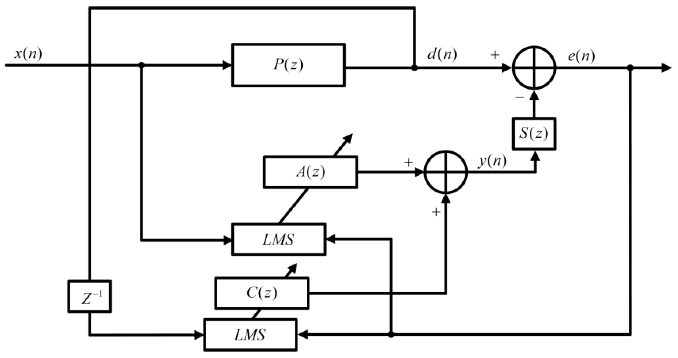
In order to solve the problem of acoustic feedback, a feedback structure is added to the secondary channel based on the FxLMS algorthm. Figure 1 reveals the OE-model-based ANC system [20,21].

where $P(z)$ and $S(z)$ are the primary and secondary paths, respectively. The error signal is given by the following:

$$e\left(n\right)=d\left(n\right)-s\left(n\right)\ast y\left(n\right)$$

(1)

where $s(n)$ is the impulse response of $S(z)$, $d(n)$ is the primary noise signal, and the $‘\ast ’$ denotes the convolution operation. $y(n)$ is expressed as follows:

$$y(n)={\displaystyle \sum _{i=0}^{N_a-1}{a}_i(n)x(n-i)+{\displaystyle \sum _{j=0}^{N_c-1}{c}_j(n)y(n-j)}}$$

(2)

where, in $a_i(n)(i=0,1,\dots ,N_{a-1})$ and $c_j(n)(j=0,1,\dots ,N_{c-1})$, $N_a$ and $N_{\mathrm{c}}$ are the filter lengths. According to the OE-model-based ANC system, the weight updating processes can be expressed as follows:

$$a(n+1)=a(n)+\mu x^{\prime }(n)e(n)$$

(3)

$$c(n+1)=c(n)+\mu \widehat{y^{\prime }}(n-1)e(n)$$

(4)

where, in $\widehat{y^{\prime }}(n)=\hat{s}(n)\ast y(n-1)$ $x^{\prime }(n)=\hat{s}(n)\ast x(n)$, $a(n)={[a_0(n)a_1(n)\dots a_{N_{a-1}}]}^T$, $x(n)={[x(n)x(n-1)\dots x(n-N_a+1)]}^T$, $c(n)=[c_1(n)c_2(n)\dots c_{N_c}(n)]$, $\hat{s}(n)$ represents the impulse response of the secondary path $\hat{S}(z)$, and $\mu$ is the step size. Meanwhile, the optimal $C(z)$ and $A(z)$ must satisfy

$$\frac{A(z)}{1-C(z)}=\frac{P(z)}{S(z)}$$

(5)

to minimize the error signal $e(n)$.

3. The EE Adaptive IIR-Filter-Based ANC Algorithm

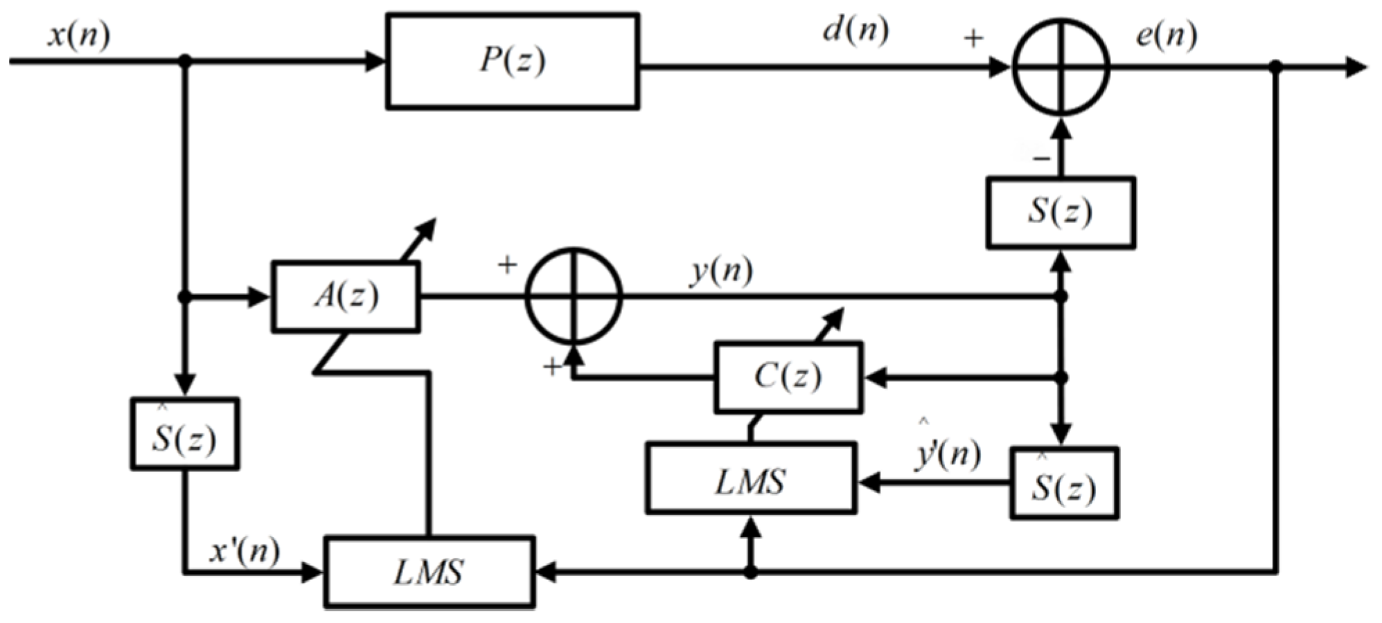
In order to solve the pole problem caused by $S(z)$ in the system shown in Figure 2, the estimated value of the desired signal $d(n)$ is synthesized by means of digital signal processing. As shown in Figure 2, the impulse response $s(n)$ of the secondary path is $S(z)$. $s(n)=[s_0{s}_1\dots s_{L-1}]$, and the output signal can be expressed as follows:

$$y(n)=a^T(n)x(n)+c^T(n)d(n-1)$$

(6)

where $d(n-1)={[d(n-1)d(n-2)\dots d(n-N_c)]}^T$. The adaptations of the EE ANC system [21] can be derived as follows:

$$a(n+1)=a(n)+\mu e(n)(\hat{s}(n)\ast x(n))$$

(7)

and

$$c(n+1)=c(n)+\mu e(n)\widehat{d^{\prime }}(n)$$

(8)

Practically, we synthesize $\hat{d}(n)=e(n)+y(n)\ast \hat{s}(n)$ instead it. Therefore, the output signal can be rewritten as follows:

$$y(n)=a^T(n)x(n)+c^T(n)\hat{d}(n)$$

(9)

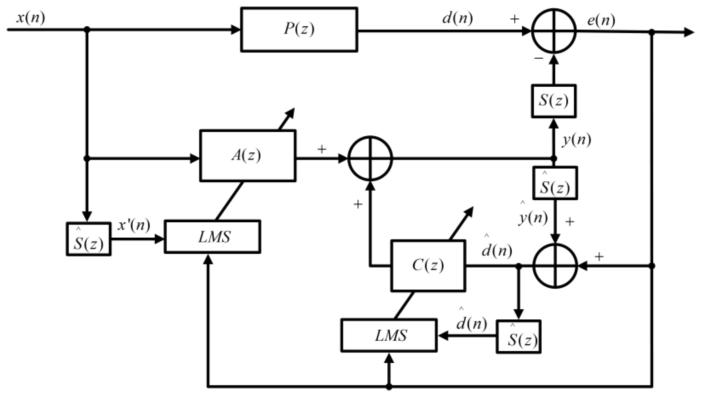
The complete ANC system block diagram based on the EE model is shown in Figure 3. As the EE model is composed of non-recursive terms, instability would be avoided. However, there are still problems such as a slow convergence speed and poor noise reduction performance.

4. The EE Adaptive IIR-Filter-Based ANC Algorithm

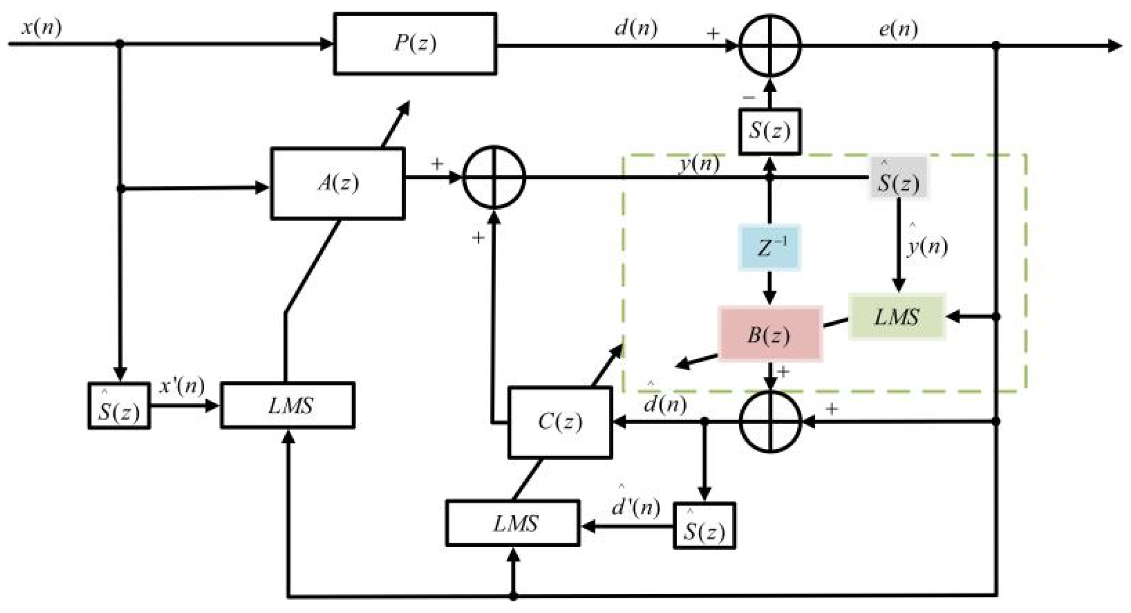
In order to improve the convergence speed and noise reduction performance of the EE-based ANC system, an improved ANC system based on EE is proposed [18], where only two adaptive filters, $A(z)$ and $C(z)$, are employed. Here, we adopt an extra filter named $B(z)$. As shown in Figure 4, $A(z)$, $B(z)$, and $C(z)$ are the transversal adaptive filters for the EE-based model. The dotted square denotes the proposed secondary path modeling. The squared error signal expressed as ${\epsilon }_{EE}^{\prime }=e^2(n)$, and the gradient of error surface is denoted as follows [18]:

$$\nabla {\epsilon }_{EE}^{\prime }=-2e(n)(s(n)\ast u(n))$$

(10)

where $s(n)$ is the impulse response of the secondary path $S(z)$ and the input of the adaptive filter is $u(n)=\left(\begin{array}{l}x(n)\\ d(n-1)\end{array}\right)$. The estimated secondary path is added, so the equation becomes

$$\nabla {\epsilon }_{EE}^{\prime }=-2e(n)(\hat{s}(n)\ast u(n))$$

(11)

Adaptations of the improved EE ANC system can be derived as follows:

$$a(n+1)=a(n)+\mu e(n)(\hat{s}(n)\ast x(n))$$

(12)

$$b(n+1)=b(n)+\mu e(n)(y(n)\ast \hat{s}(n))$$

(13)

$$c(n+1)=c(n)+\mu e(n)\widehat{d^{\prime }}(n)$$

(14)

Finally, the output signal of the improved EE ANC system can be rewritten as follows:

$$y(n)=a^T(n)x(n)+c^T(n)(e(n)+b^T(n)\hat{y}(n))$$

(15)

$$\frac{A(z)}{1-C(z)B(z)}=P(z)$$

(16)

It can be seen from Equation (15) that the improved EE model can avoid instability and improve the accuracy of the synthesized $d(n)$ signal, as it is a nonrecursive system.

4.1. The Step-Size Constraint

We assume that reference signal $x(n)$ is a white noise signal with a mean value of zero and a variance of 1. The step size limits ${\mu }_A$, ${\mu }_B$, and ${\mu }_C$ of $A(z)$, $B(z)$, and $C(z)$, are set as the following Equation (16), respectively:

$$0<{\mu }_A<\frac{3}{(N_a+3{\mathsf{\Delta }}_{eq})P_{x^{\prime }}}$$

(17)

$$0<{\mu }_B<\frac{3}{(N_b+3{\mathsf{\Delta }}_{eq})P_{\hat{y}}}$$

(18)

$$0<{\mu }_C<\frac{3}{(N_c+3{\mathsf{\Delta }}_{eq})P_{\widehat{d^{\prime }}}}$$

(19)

where $P_{x^{\prime }}$, $P_{\hat{y}}$, and $P_{\widehat{d^{\prime }}}$ denote the power of $x^{\prime }(n)$, $\hat{y}(n)$, and $\widehat{d^{\prime }}(n)$, respectively, and the is the equivalent delay of the secondary path Equation (16). ${\mathsf{\Delta }}_{\mathrm{eq}}$ can be expressed as follows:

$${\mathsf{\Delta }}_{\mathrm{eq}}=\frac{{\displaystyle \sum _{l=1}^{L-1}l{s}_l^2}}{{\displaystyle \sum _{l=0}^{L-1}{s}_l^2}}$$

(20)

The maximum overall step-size $\mu$ of the ANC system should be the minimum of ${\mu }_A$, ${\mu }_B$, and ${\mu }_C$, and the signal powers of $P_{x^{\prime }}$, $P_{\hat{y}}$, and $P_{\widehat{d^{\prime }}}$ in Equations (16)–(18) are set to be 1. Hence, the maximum step size and filter length are only affected by the secondary path delay ${\mathsf{\Delta }}_{\mathrm{eq}}$.

4.2. Global Minimum Solutions

The mean square error (MSE) function based on the improved EE-based ANC system is expressed as follows:

$$\begin{array}{ll}{\xi }_{EE}^{\prime }(n)& =E[d^2(n)]+a^T(n)R_{x^{\prime }{x}^{\prime }}a(n)\\ & +b^T(n)R_{\hat{y}\hat{y}}b(n)+c^T(n)R_{\widehat{d^{\prime }}\widehat{d^{\prime }}}c(n)\\ & +2[a^T(n)R_{x^{\prime }\widehat{d^{\prime }}}c(n)+a^T(n)R_{x^{\prime }\hat{y}}b(n)\\ & +b^T(n)R_{\hat{y}\widehat{d^{\prime }}}c(n)-a^T(n)p_{d{x}^{\prime }}-b^T(n)p_{d\hat{y}}\\ & -c^T(n)p_{d\widehat{d^{\prime }}}]\end{array}$$

(21)

where $R_{x^{\prime }{x}^{\prime }}=E[x^{\prime }(n)x^{\prime T}(n)]$, $R_{\hat{y}\hat{y}}=E[\hat{y}(n)\hat{y}(n)]$, $R_{\widehat{d^{\prime }}\widehat{d^{\prime }}}=E[x^{\prime }(n)x^{\prime T}(n)]$, $R_{x^{\prime }\widehat{d^{\prime }}}=E[x^{\prime }(n)\widehat{d^{\prime T}}(n)]$ and $p_{d{x}^{\prime }}=E[d(n)x^{\prime }(n)]$ $p_{d\widehat{d^{\prime }}}=E[d(n)\widehat{d^{\prime }}(n)]$. It can be seen that the ANC system based on the improved EE model owns a global minimum. By calculating the gradient function of Equation (21), we have

$$\begin{array}{ll}\frac{\partial {\xi }_{EE}^{\prime }}{\partial a(n)}& ={[\frac{\partial {\xi }_{EE}^{\prime }(n)}{\partial a_0(n)}\frac{\partial {\xi }_{EE}^{\prime }(n)}{\partial a_1(n)}\cdot \cdot \cdot \frac{\partial {\xi }_{EE}^{\prime }(n)}{\partial a_{N_{a-1}}(n)}]}^T\\ & =2R_{x^{\prime }{x}^{\prime }}a(n)+2R_{x^{\prime }\widehat{d^{\prime }}}c(n)+R_{x^{\prime }\hat{y}}b(n)-2p_{d{x}^{\prime }}\end{array}$$

(22)

$$\begin{array}{ll}\frac{\partial {\xi }_{EE}^{\prime }(n)}{\partial b(n)}& ={[\frac{\partial {\xi }_{EE}^{\prime }(n)}{\partial b_0(n)}\frac{\partial {\xi }_{EE}^{\prime }(n)}{\partial b_1(n)}\cdot \cdot \cdot \frac{\partial {\xi }_{EE}^{\prime }(n)}{\partial b_{N_{a-1}}(n)}]}^T\\ & =2R_{\hat{y}\hat{y}}b(n)+2R_{x^{\prime }\hat{y}}a(n)+2R_{\hat{y}\widehat{d^{\prime }}}c(n)-2p_{d\hat{y}}\end{array}$$

(23)

$$\begin{array}{ll}\frac{\partial {\xi }_{EE}^{\prime }(n)}{\partial c(n)}& ={[\frac{\partial {\xi }_{EE}^{\prime }(n)}{\partial c_0(n)}\frac{\partial {\xi }_{EE}^{\prime }(n)}{\partial c_1(n)}\cdot \cdot \cdot \frac{\partial {\xi }_{EE}^{\prime }(n)}{\partial c_{N_{a-1}}(n)}]}^T\\ & =2R_{\widehat{d^{\prime }}\widehat{d^{\prime }}}c(n)+2R_{x^{\prime }\widehat{d^{\prime }}}{a}^T(n)+2b^T(n)R_{\hat{y}\widehat{d^{\prime }}}-2p_{d\widehat{d^{\prime }}}\end{array}$$

(24)

Therefore, the optimal weight vectors, $a_{EE}^0(n)$ $b_{EE}^0(n)$, and $c_{EE}^0(n)$ can be derived by supposing that the gradient functions are equal to zero.

5. Computer Simulation

5.1. Test Environment and Noise Characteristics

The noise of the compressor (product model VW-11/4) in a gas station is $x(n)$, which possesses a strong periodicity and high noise input level. As shown in Figure 5a, a dual-channel audio signal analyzer (AWA6290M+) is used to transmit the audio signals collected by two signal sensors to the MATLAB2019a software on a personal computer for algorithm verification processing. The distance from $senso{r}_1$ to the computer is the primary path (1.2 m), and the distance from $senso{r}_0$ to the computer is the secondary path (6.7 m).

The time–frequency diagram of the tested noise is obtained by the computer measurement system shown in Figure 5b, indicating that the sound pressure level in the low frequency range of 0–1 kHz is much higher than the one in the high frequency range. To compare our algorithm with the ones in [1,5,18] under similiar conditions, the secondary path of this system is set with a delay of 24 samples and filter length of 64.

5.2. Simulation Results

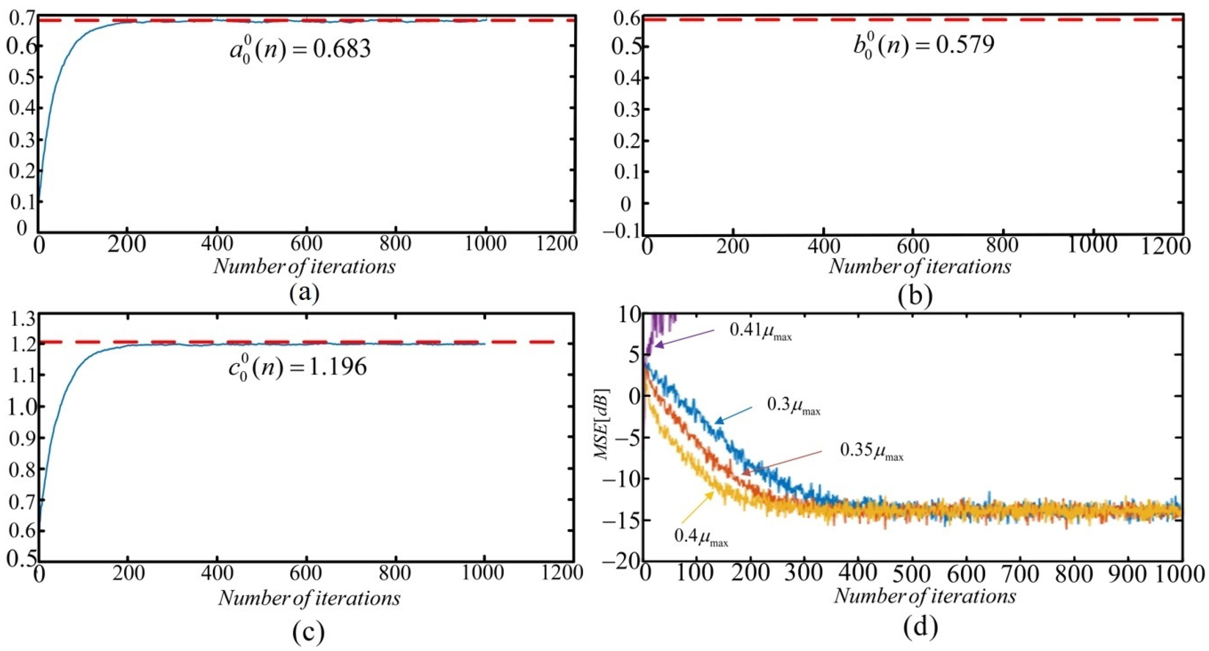
Firstly, by inputting the data into Equations (12)–(14) of the improved EE-based ANC system model, the learning process of the weight coefficients can be calculated as shown in Figure 6a–c. Moreover, we can compute the optimal weights $a_0^0(n)=0.683$, $b_0^0(n)=0.579$, and $c_0^0(n)=1.196$ (the first column vector of the optimal weight coefficient matrix). Secondly, according to Equations (17)–(20), the step size bounds can be computed as ${\mu }_A<0.139$, ${\mu }_B<0.346$, and ${\mu }_C<0.21$.

Therefore, the step size bound is $\mu <0.139$, i.e., ${\mu }_{\max }=0.139$. The learning curves with different step sizes are shown in Figure 6d, and is achieved by applying the following Equation (22):

$$\partial (n)=\gamma \partial (n-1)+(1-\gamma )e^2(n)$$

(25)

where $\gamma =0.97$ is a forgetting factor. By taking $n=0$, we have $\partial (0)=e^2(0)$. The improved EE-based ANC system converges when the step size is less than $0.4{\mu }_{\max }$.

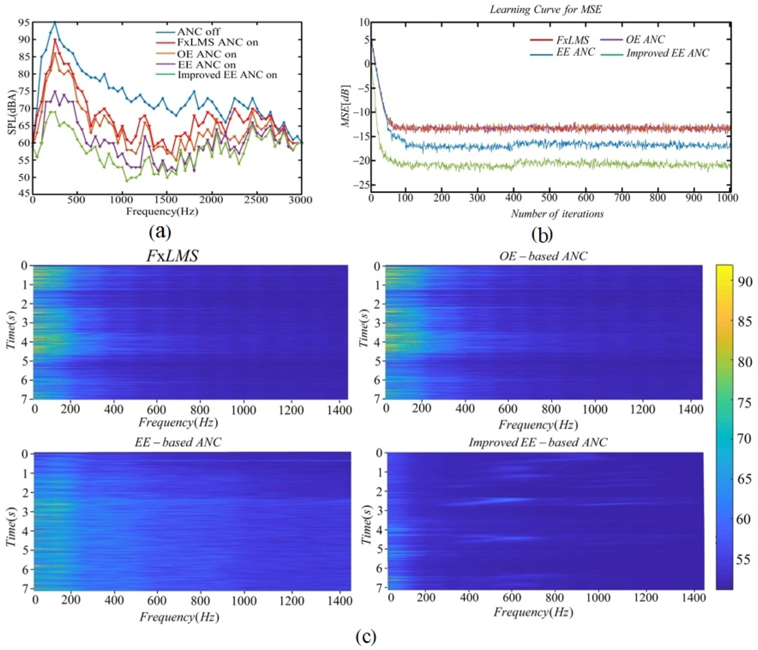
We compare the performance of the conventional FIR method (FxLMS), the OE-based model, the EE-based ANC systems in [12,17,18], and the improved EE-based ANC systems with the measurement noise. Figure 7a reveals the average sound pressure level of the noise. The step sizes are 0.018, 0.015, 0.0016, and 0.0007 for the FxLMS, OE, EE, and improved EE schemes, respectively. The FxLMS-based algorithm filter length is 200; the filter lengths of $A(z)$ and $C(z)$ are 42 for both the OE-based and EE-based ANC systems; and the filter lengths of $A(\mathrm{z})$, $B(z)$, and $C(z)$ are 42 for the improved EE-based system. Obviously, the algorithms compared in this paper can effectively converge and achieve a certain noise reduction effect. Although, for the noise of a compressor, the improved EE-based ANC system shows better convergence speed, as shown in Figure 7b. Furthermore, as shown in Figure 7a, the improved ANC system can reduce the noise of the compressor up to 28 dBA at frequency below 2.5 kHz, and the amplitude is expressed by the A-weighted sound pressure level. In addition, the time–frequency diagram of the ANC system through various algorithms is shown in Figure 7c.

5.3. Computational Complexity

We compare the calculation complexity of the FIR-based FXLMS algorithm, the IIR-based OE, the EE-based ANC system, and the improved EE-based ANC system in

Table 1. Computational complexity.

Algorithm	Multplications	Additions
FxLMS	$2N+L+2$	$2N+L-1$
OE ANC	$2N_{\mathrm{a}}+2N_c+2L+2$	$2N_{\mathrm{a}}+2N_c+2L-2$
EE ANC	$2N_{\mathrm{a}}+2N_c+3L+2$	$2N_{\mathrm{a}}+2N_c+3L-2$
Proposed EE ANC	$2N_{\mathrm{a}}+2N_{\mathrm{b}}+2N_c+4L+2$	$2N_{\mathrm{a}}+2N_b+2N_c+4L-2$

. The filter lengths of $W(z)$, $A(z)$, $B(z)$, and $C(z)$ are $N$, $N_{\mathrm{a}}$, $N_{\mathrm{b}}$, and $N_c$, respectively. Generally speaking, in contrast with the FIR-based method, the IIR-based method can utilize fewer filter lengths; in comparison with the OE-based method, the EE-based method requires an additional filtering of $\hat{S}(z)$ to obtain the output signal; in contrast with the EE-based method, the improved EE-based method adds an additional adaptive filter $C(z)$ in order to make the ANC system more accurate and faster.

Table 1 displays the comparison of the computational complexity of the various algorithms. If we substitute the previous data into the table using the FxLMS algorithm for 450 multiplications and 447 additions, the OE-based method requires 298 multiplications and 294 additions, the EE-based method needs 362 multiplications and 358 additions, and the improved EE-based method requires 424 multiplications and 420 additions. Obviously, the IIR-based models cost less in computational complexity.

6. Conclusions

This paper introduces an adaptive IIR filter based on an improved EE model employing an offline secondary path modeling method that is superior in convergence speed and noise reduction performance. The compressor noise is taken as the input noise data to simulate the performance of the system. The results show that it has a good noise reduction effect from 0 Hz to 2.5 kHz. However, the system will increase a certain amount computational complexity. The model proposed in this paper is suitable for processing noise signals in a low frequency range, which is typical among industrial equipment, such as engines and compressors with loud noise signals.

References

- Lasota, A.; Meller, M. Iterative Learning Approach to Active Noise Control of Highly Autocorrelated Signals with Applications to Machinery Noise. IET Signal Process. 2020, 14, 560–568. [Google Scholar] [CrossRef]
- Nelson, P.A.; Elliott, S.J.; John, E.W.F. Active control of sound basics of interferometry. Phys. Today 1993, 46, 75. [Google Scholar] [CrossRef]
- Fredianelli, L.; Del Pizzo, A.; Licitra, G. Recent developments in sonic crystals as barriers for road traffic noise mitigation. Environments 2019, 6, 14. [Google Scholar] [CrossRef] [Green Version]
- Koussa, F.; Defrance, J.; Jean, P.; Blanc-Benon, P. Acoustical efficiency of a sonic crystal assisted noise barrier. Acta Acust. United Acust. 2013, 99, 399–409. [Google Scholar] [CrossRef] [Green Version]
- Kuo, S.M.; Morgan, D.R. Active Noise Control Systems; Wiley: New York, NY, USA, 1996; Volume 4. [Google Scholar]
- Aggogeri, F.; Al-Bender, F.; Brunner, B.; Elsaid, M.; Mazzola, M.; Merlo, A.; Ricciardi, D.; De La ORodriguez, M.; Salvi, E. Design of piezo-based avc system for machine tool applications. Mech. Syst. Signal Process. 2013, 36, 53–65. [Google Scholar] [CrossRef]
- Guo, X.; Jiang, J.; Chen, J.; Du, S.; Tan, L. Bibo-stable implementation of adaptive function expansion bilinear filter for nonlinear active noise control. Appl. Acoust. 2020, 168, 107407. [Google Scholar] [CrossRef]
- Lam, B.; Shi, C.; Shi, D.; Gan, W.S. Active control of sound through full-sized open windows. Build. Environ. 2018, 141, 16–27. [Google Scholar] [CrossRef]
- Murao, T.; Shi, C.; Gan, W.S.; Nishimura, M. Mixed-error approach for multi-channel active noise control of open windows. Appl. Acoust. 2017, 127, 305–315. [Google Scholar] [CrossRef]
- Shi, C.; Jia, Z.; Xie, R.; Li, H. An active noise control casing using the multi-channel feedforward control system and the relative path based vir-tual sensing method. Mech. Syst. Signal Process. 2020, 144, 106878. [Google Scholar] [CrossRef]
- Carini, A.; Mathews, V.J.; Sicuranza, G.L. Sufficient stability bounds for slowly varying direct-form recursive linear filters and their applications in adaptive iir filters. IEEE Trans. Signal Process. 1999, 47, 2561–2567. [Google Scholar] [CrossRef]
- Feng, D.Z.; Zheng, W.X. Fast rls-type algorithm for unbiased equation-error adaptive iir filtering based on approximate inverse-power iteration. IEEE Trans. Signal Process. 2005, 53, 4169–4185. [Google Scholar] [CrossRef]
- Netto, S.L.; Diniz, P.S.; Agathoklis, P. Adaptive iir filtering algorithms for system identification: A general framework. IEEE Trans. Educ. 1995, 38, 54–66. [Google Scholar] [CrossRef]
- Regalia, P. Adaptive IIR Filtering in Signal Processing and Control; Rout-ledge: London, UK, 2018. [Google Scholar]
- Mandelbrot, B.B. The variation of certain speculative prices. In Fractals and Scaling in Finance; Springer: Berlin, Germany, 1997; pp. 371–418. [Google Scholar]
- Bouvet, M.; Schwartz, S.C. Comparison of adaptive and robust receivers for signal detection in ambient underwater noise. IEEE Trans. Acoust. Speech Signal Process. 1989, 37, 621–626. [Google Scholar] [CrossRef]
- Elliott, S.; Nelson, P. The active control of sound. Electron. Commun. Eng. J. 1990, 2, 127–136. [Google Scholar] [CrossRef]
- Ho, C.Y.; Shyu, K.K.; Chang, C.Y.; Kuo, S.M. Development of equation-error adaptive iir-filter-based active noise control system. Appl. Acoust. 2020, 163, 107226. [Google Scholar] [CrossRef]
- Zhao, T.; Liang, J.; Zou, L.; Zhang, L. A new fxlms algorithm with offline and online secondary-path modeling scheme for active noise control of power transformers. IEEE Trans. Ind. Electron. 2017, 64, 6432–6442. [Google Scholar] [CrossRef]
- Kim, I.S.; Na, H.S.; Kim, K.J.; Park, Y. Constraint filtered-x and filtered-u least-mean-square algorithms for the active control of noise in ducts. J. Acoust. Soc. Am. 1994, 95, 3379–3389. [Google Scholar] [CrossRef]
- Fraanje, R.; Verhaegen, M.; Doelman, N. Convergence analysis of the filtered-u lms algorithm for active noise control in case perfect cancellation is not possible. Signal Process. 2003, 83, 1239–1254. [Google Scholar] [CrossRef]
Figure 1.
The output-error (OE)-model-based active noise control (ANC) system using the FURLMS algorithm.
Figure 2.
ANC system based on an equation error (EE) adaptive infinite-impulse-response (IIR) filter.
Figure 3.
Complete block diagram of the ANC system when applying an EE adaptive IIR filter.
Figure 4.
The improved EE adaptive IIR-filter-based ANC algorithm.
Figure 5.
(a) Test environment; (b) time–frequency graph of the collected noise in a certain period of time.
Figure 6.
Convergence process of weight coefficients (a–c) and ANC system based on improved EE in different step factors (d).
Figure 7.
(a) Indicates the noise reduction performance comparison of different ANC systems, the ordinate is the A-weighted sound pressure level, and the abscissa is the frequency. (b) The convergence process of the mean square error of each algorithm. (c) Time–frequency diagram of different algorithms after noise reduction.