Application of Bayesian Hierarchical Finite Mixture Model to Account for Severe Heterogeneous Crash Data

Abstract

Various techniques have been proposed in the literature to account for the observed and unobserved heterogeneity in the crash dataset. Those include techniques such as the finite mixture model (FMM), or hierarchical techniques. The FMM could provide a flexible framework by providing various distributions for various individual observations. However, the shortcoming of the standard FMM is that it cannot account for the heterogeneity in a single model’s structure, and the data needs to be disaggregated to its resultant subsamples. That would result in a loss of information. On the other hand, a second plausible approach is to use a hierarchical technique to account for the data heterogeneities, being based on various explanatory variables, and based on engineering intuition. In the context of traffic safety, while some researchers, for instance, considered the seasonality, some others considered highway systems or even genders. However, a question might arise: are the same observations within a same hierarchy homogenous? Are all the observations within different clusters heterogeneous? Additionally, how about other variables? Although the results in the literature highlighted accounting for the structure of the dataset would result in an acceptable interclass correlation (ICC), and also result in a significant improvement in terms of reduction in the deviance information criteria (DIC), there is no justification why to use those specific hierarchies and reject others. A more reasonable approach is to let the algorithm come up with the best distributions based on the provided parameters and accommodate observations to the related mixtures. In that approach those observations that belong to various subjective hierarchies, e.g., winter versus summer, but found to be similar would be set in a similar cluster. That is why we proposed this methodology to implement an objective hierarchy of the FMM to be used for the hierarchical technique. Here, due to the label switching problem of the FMM in the context of Bayesian, the FMM first conducted in the context of maximum likelihood estimates, and then assigned observations were used for the final analysis. The results of the DIC highlighted a significant improvement in the model fit compared with a subjective assigned hierarchy based on highway system. Additionally, although the subjective model resulted in a very low ICC due to so much heterogeneity in the dataset, the implemented methodology resulted in an acceptable ICC (0.3), justifying the use of hierarchy. The Bayesian hierarchical finite mixture model (BHFMM) is one of earliest application in traffic safety studies. The findings of this study have important implications for the future studies to account for a higher heterogeneity of the crash dataset based on the distance of observations to each cluster.

1. Introduction

Vehicle crashes are one of the leading causes of death around the world. Annually, more than 1 million people die and more than 20 million are severely injured in crashes [1]. These crashes are ranked 7th in terms of life lost [2]. The life lost is equivalent to more than 230 billion worth of crash costs every year.

Researchers around the world are striving to find and tackle contributory factors to crashes in the most accurate way by implementing advanced statistical techniques, especially by accounting for the data heterogeneity. One of the main sources of data heterogeneity is due to not accounting for the structure of the data. This would ignore the similarities across observations in the same group, and dissimilarly across the cross-group resulting in data heterogeneity.

Researchers, especially, in social science are often confronted with hierarchical data. Examples are numerous such as: repeated measures taken from the same individuals in an organization, individuals living in a same state with various districts and so on. Despite the obvious structures in those fields, very often the researchers consider the hierarchical techniques for traffic safety studies. Although no clear-cut structures could be assigned to the dataset, often various factors such as seasonality, gender, highway, or barrier types have been considered. As it is expected, almost all those studies highlighted an improvement in the model fit. However, the question might arise whether those variables could account for optimum amount of the heterogeneity in the datasets. If, for instance, the highway system was chosen as the hierarchy levels, would all the observations within each highway system be similar, and would the observations within various categories be different?

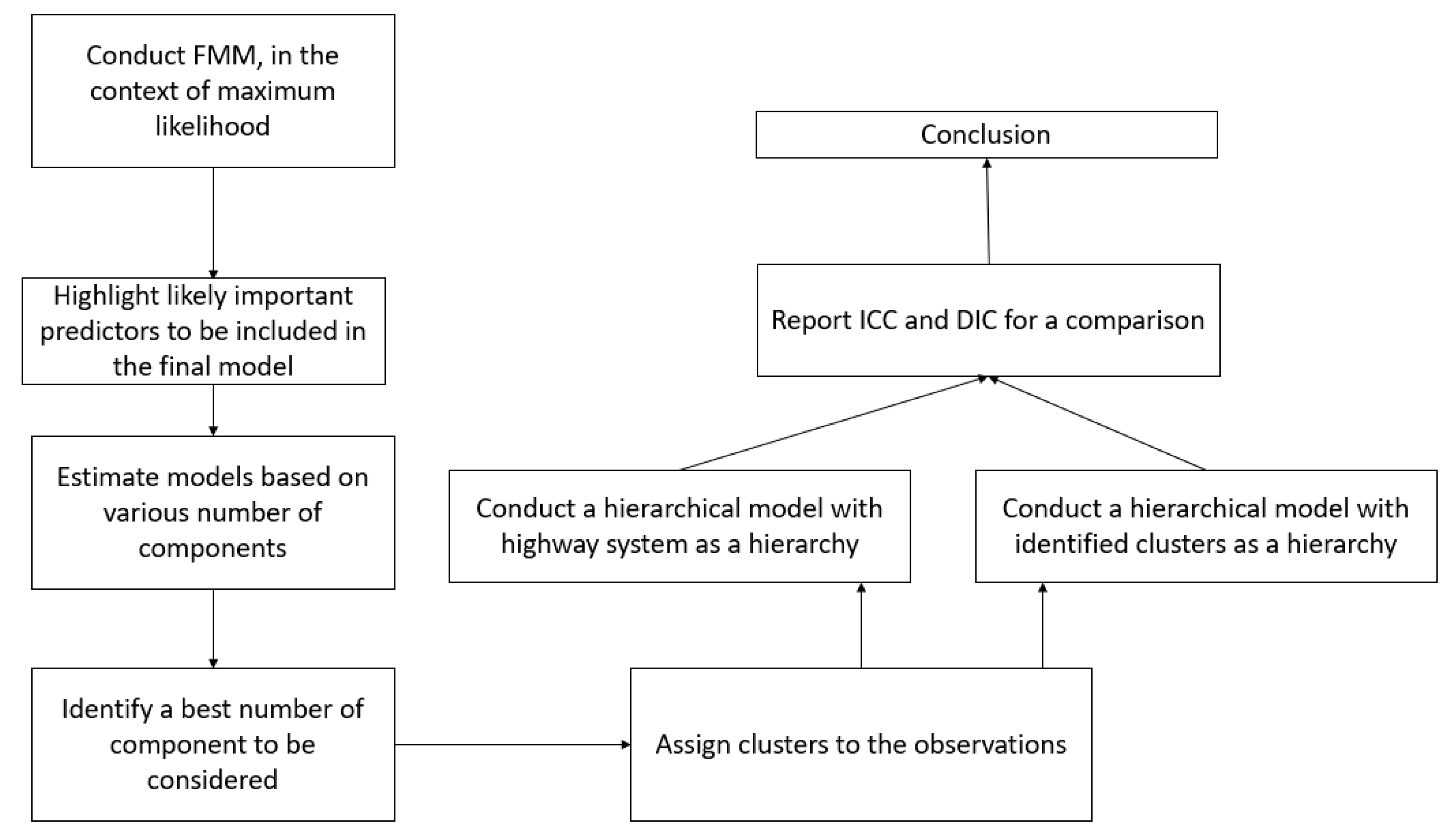
Significant efforts also have been made for the use of the finite mixture model (FMM) for the traffic studies. Based on that method, observations closest to a cluster would be assigned to that cluster accounting for the heterogeneity of the dataset. Although the method has the capability to account for the data heterogeneity, it would result in a loss of information. Thus, in this study we took advantage of both methods by aggregating those techniques. The method is the Bayesian hierarchical finite mixture model (BHFMM). The methodological approach is described in Figure 1. A comprehensive discussion was made, and the methodological approach presented in Figure 1.

The content of this manuscript is structured as follows: the method section would discuss the methodological approaches taken in this study followed by the data section, which details the data used in this study. The findings are then summarized in the results section.

2. Method

This section describes the methodological approach implemented in this study. It, first, briefly discusses the model distributions being considered in this study. It then covers the FMM technique. The methodological approach then discusses how the models’ parameters would be estimated.

2.1. Model Distributions

The negative binomial, gamma–Poisson model, is equivalent to the Poisson distributions with mean parameter $\mu$, where the $\mu$ parameter follows a gamma distribution with shape parameter $\alpha$, and rate parameter of $\alpha /\mu$. Although maximum likelihood has been used extensively in the literature by the generalized linear model (GLM), the Bayesian model especially favors the data, if there is prior expert knowledge about the parameters of interest, or when especially there is a small sample size.

Although we did not have any prior knowledge about the possible distributions’ parameters of interest, the hierarchical technique was used due to a relatively low number of observations, and ease of implementing the hierarchical technique in the Bayesian context. In this paper, a hierarchical approach has been developed where there were 3 levels of hierarchy due to the factor of cluster.

Often, the response variable is a count response, which makes the algorithm for estimating the parameters more challenging, compared with a binary response like Probit or logit models. For this model we have a set of covariates as x = ${\left[1,x_1,\dots ,x_p\right]}^T$, and coefficients as $\beta ={[{\beta }_0,\dots ,{\beta }_p]}^T$. Compared with the Poisson model, where the mean and variance are both equal to λ, in this study due to reasons such as differences across the individual observations, crash count, the model would be characterized as overdispersed, having a variance greater than the mean. To address the shortcoming of the Poisson model, the NB model could be used by placing a gamma distribution prior with the shape of $\alpha$ and scale of $\frac{p}{1-p}$ so we would have:

$$f\left(r,p\right)={\int }_0^{\infty }{f}_{Poisson\left(\lambda \right)}{f}_{Gamma}\left(\alpha ,\frac{1-P}{P}\right)d\lambda ,$$

(1)

where $\lambda$ is the only parameter of Poisson, while there are two parameters of shape and scale for gamma.

The probability density function (PDF) of the Poisson–gamma mixture, from Equation (1), would be written as:

$$P(Y=y_i|{\lambda }_i,\alpha )=\frac{\mathsf{\Gamma }\left(y_i+{\alpha }^{}\right)}{\mathsf{\Gamma }\left(y_i+1\right)\mathsf{\Gamma }\left({\alpha }^{}\right)}{\left(\frac{{\alpha }^{}}{{\alpha }^{}+{\lambda }_i}\right)}^{{\alpha }^{}}{\left(\frac{{\lambda }_i}{{\alpha }^{}+{\lambda }_i}\right)}^{y_i},$$

(2)

where $\mathsf{\Gamma }(.)$ is the gamma function, P is a probability parameter, and Y is assumed to follow the negative binomial (NB) distribution through the log link function.

Now based on the above, the posterior probability of beta conditioned on data could be obtained as:

$$P\left(\beta |data\right)=\frac{P\left(\beta \right)P(data|\beta )}{\int P\left(\beta \right)d\beta },$$

(3)

As the equation $P(data|\beta )$ in the numerator is intractable, after denoting distributions to the parameter’s prior, a simulation-based approach would be used for estimating the posterior distributions of $\beta$.

The log likelihood function for finding the model parameters of the above equation could be written as follows [3]:

$$ℒ={\displaystyle \sum }_{i=1}^n\{\ln \left[\mathsf{\Gamma }\left(y_i+{\alpha }^{-1}\right)\right]-\ln [\left(\mathsf{\Gamma }\left({\alpha }^{-1}\right)\right]-\ln \left[\mathsf{\Gamma }\left(y_i+1\right)\right]-{\alpha }^{-1}\ln \left(1+\mathsf{\alpha }{\mu }_i\right)-y_i\ln \left(1+\left(\alpha {\mu }_i\right)\right)+y_i\ln \left(\alpha \right)+y_i\ln \left({\mu }_i\right)$$

(4)

The above is the key for the parameters’ estimates in the context of maximum likelihood estimation, which would be solved with the help of gradient and Hessian. In the Bayesian context the process is based on sampling, which an upcoming subsection would talk about.

2.2. Finite Mixture Model

The FMM with K components would be written as follows [4]:

$$h\left(y|x,\phi \right)={\displaystyle \sum }_{k=1}^K{\pi }_{k}f(y|x,{\theta }_k)$$

(5)

where y is a dependent variable, with conditional density h, x is a vector of independent variable, and ${\pi }_k$ is dependent on the number of clusters or groups.

$\phi$ is a vector of all the parameters as:

$$\phi =\left({\pi }_1\dots .,{\pi }_K,{\overline{\theta }}_1,\dots ,{\overline{\theta }}_K\right)$$

(6)

Consider $f$ as a normal density, for instance, with two parameters of mean as $\overline{\mu }$ and variance of ${\sigma }^2$. ${\theta }_k$ could be written as ${\overline{\theta }}_K=\left(\overline{\mu }, {\sigma }^2\right)$, and in the above equation, h could be called as latent class regression [5]. On the other hand, if $f$, like our case, is a member of the exponential family, the model would be a mixture of generalized linear models [6].

The posterior probability that a crash (x, y) belongs to class j is [4]:

$$P\left(j|x,y,\phi \right)=\frac{{\pi }_{i}f(y|x,{\theta }_j)}{{\sum }_k{\pi }_{k}f(y|x,{\theta }_k)}$$

(7)

The log likelihood of a mixture multivariate model with N observations {($x_1,y_1$),…, ($x_N,y_N$) could be written as:

$$\log ℒ={\displaystyle \sum }_{n=1}^N\log h\left(y_n|x_n,\phi \right)$$

(8)

After interposing h, from Equation (5) in the above equation, there would be:

$$\log ℒ={\displaystyle \sum }_{n=1}^N\log ({\displaystyle \sum }_{k=1}^K{\pi }_{k}f(y|x_n,{\theta }_k)$$

(9)

The above equation would be implemented across various observation crashes, of n belonging to a component k. The above equation cannot be solved directly, so, it would be solved based on the expectation-maximization (EM) algorithm. In summary, the likelihood of each component would be maximized separately by using a posterior probability,${\widehat{p}}_{nk}$, as weights:

$${}_{{\theta }_k}{}^{max}\widehat{p}{}_{nk}\log f(y_n|x_n,{\theta }_k)$$

(10)

Additionally, ${\widehat{p}}_{nk}$ could be written as:

$${\widehat{p}}_{nk}=P(k|x_n,y_n,\widehat{\phi })$$

(11)

where k is the component.

The FMM highlights that in an efficient way, the traffic barriers could be considered to be obtained, for instance, from 4 different negative binomial distributions. Additionally, those distributions are not necessarily based on barrier types or highway classifications.

Research have implemented various techniques to account for the heterogeneity of the data. These include methods such as separating the dataset based on various characteristics such as highway systems or accounting for the heterogeneity through considering the mixed effect model. Although these two methods could account for the heterogeneity of the dataset, they could not account for the heterogeneity in a most efficient way.

Another method is to separate the dataset based on various distributions to account for an unobserved heterogeneity in a most efficient way. In other words, after randomly assigning a number of k as components, the model would come up with k distributions. Observations closest to a cluster would be assigned to that cluster. After assigning all the observations to each component, weighted generalized linear model (GLM) model, with the assigned distribution would be conducted. This is a model-based clustering. Barriers data could be clustered into 4 separate equations, for instance, in a most efficient way as follows:

$$P\left(X|\lambda ,\alpha \right)=n_1\mathrm{NB}\left(X_a|{\lambda }_1,{\alpha }_1\right)+n_2\mathrm{NB}\left(X_b|{\lambda }_2,{\alpha }_2\right)+n_3\mathrm{NB}\left(X_c|{\lambda }_3,{\alpha }_3\right)+n_4\mathrm{NB}\left(X_d|{\lambda }_4,{\alpha }_4\right)$$

(12)

where $X_a,X_b,X_c, \mathrm{and} X_d$ are the observations belonging to 4 clusters. $\lambda \mathrm{and} \alpha$ are negative binomial model parameters.

To make Equation (12) more intuitive, consider 2 component models with the x number of distributions: while the first model follows an equation of y = 5 + 2x, the second component follows the equation of y = 0.5 + 3x. After using the EM algorithm, appropriate distribution would be identified, and points/observations would be assigned to the appropriate clusters with the higher probability. In other words, observations would be assigned to the model distributions by answering the question of: what is the likelihood that the ith observation comes from k component $p(x_i|z_i=k,r_2,p_2)$: Observation belongs to a cluster with a highest probability. Recall that the shortcoming of the application of Equation (12) is the loss of information due to separating the dataset into k number of datasets. A discussion why the FMM was conducted in the maximum likelihood context would be presented in a future subsection.

2.3. Model Parameters’ Estimations

It can be said that the objective clustering associated with the FMM technique, identifies subsets of features that could best discriminate the observation crashes, while considering sets of covariates associated for each class. Contrary to frequentist methods, Bayesian methods consider the probability as beliefs. Non informative belief by a prior distribution would be given to an unknown parameter $\theta$ as $\pi \left(\theta \right)$. After seeing various data observations, based on the Bayes theorem, we would have:

$$\pi (\theta |X_1,\dots ,X_1)~ℒ\left(\theta \right)\pi \left(\theta \right)$$

(13)

where $ℒ\left(\theta \right)$ is the likelihood function.

In summary, in simple words, the process of the MCMC, based on the above equation, would be highlighted in few points as:

• Express the belief with a probability density (prior distribution) $\pi \left(\theta \right)$, this is without seeing any data.
• Now distributions such as negative binomial or logit models would be highlighted to reflect our beliefs about x given $\theta$;
• After observing data {$X_1,\dots ,X_n\}$, our beliefs would be updated for estimation of the posterior distribution p$(\theta |X_n)$.

However, the challenge in the computation of multiparameter problems is, there would be a need to extract inferences about few parameters instead of only a single parameter. Due to difficulty in calculating the integral, the simulation could be used for solving the integral by randomly drawing from the posterior. For instance, for estimating the marginal posterior for ${\theta }_1$ we would have:

$$p({\theta }_1|D_n)={\displaystyle \int }\dots {\displaystyle \int }p({\theta }_1,\dots ,{\theta }_d|D)d{\theta }_2,\dots ,d{\theta }_d$$

(14)

Suppose that $p$ is a family of prior distributions, and for each $\theta$ we have a distribution $p(.|\theta )$, then we have:

$$p(\theta |x)=\frac{p(x|\theta )\pi \left(\theta \right)}{\int p(x|\theta )\pi \left(\theta \right)d\theta }$$

(15)

It should be noted that often we need to sample from a complicated distribution h to reach our objective of posterior distribution. However, we would draw samples from a simplified distribution, which, based on the law of large number, would be converged to a desired distribution. For instance, consider a complicated function h. We could instead sample from a uniform distribution of U (0, 1) for estimating the integral, and based on the assumption of large number, we could assume the model would converge to the desired integral.

Importance sampling is a basic concept of Monte Carlo that addresses the challenge that there is no guarantee that the sampling, likelihood function, is from a known distribution. For instance, consider g is a probability density that we know how to sample from, and f is the probability density, which we do not know how to sample from, we have:

$$I={\displaystyle \int }h\left(x\right)f\left(x\right)dx={\displaystyle \int }\frac{h\left(x\right)f\left(x\right)}{g\left(x\right)}g\left(x\right)d\left(x\right)={\mathbb{E}}_g\left(Y\right)$$

(16)

Again, by the law of large number for the above we have $\widehat{I}\to I$.

The Gibbs sampling would be used to find the conditional distribution of a parameter, conditioned on all other parameters. The concept is by gathering information and receiving feedbacks from the model, we would refine our belief to get closer to the truth. That follows a Bayes theorem. The knowledge of various explanatory variables would update our beliefs about the status of the crash counts. Thus, by gathering more information and updating the beliefs we can get closer to the truth.

The idea behind the Markov chain is that the random samples are generated by a special sequential process. In other words, the next random sample would be generated based on a previous generated value. It should be noted that although each new sample is dependent on the before samples, new samples are not dependent on the ones before the previous.

The process with Gibbs sampling could be summarized as follows:

• Begin with the starting values.
• Generate a new proposal by taking the last sample and adding some noise. The noise would be generated from proposal distribution, e.g., normal distribution with a mean of zero and wide precision.
• Estimate the next samples from the previous values with no rejection. Instead of the accept–reject method, or Metropolis–Hastings, we use Gibbs sampling, which is based on ${\theta }_2^{\left(j\right)}~p({\theta }_2|{\theta }_1^{\left(j\right)})$. This would be estimated with the assumed distribution. The process would be described as follows:

  ▪

  Consider, for instance, two chains with 1000 iterations with an initial value such as 1 and 1.

  ▪

  Normalize the initial values based on the data distribution and replace updated values by the assigned starting values, highlighting the plausibility of initial values that came out from the proposed distribution.

  ▪

  Generate the first value in the first chain by adding up the related starting value by some random numbers: It should be noted that the generated values are created by adding up initial values by a random number from the normal distribution, or assigned distribution.

  ▪

  Check the plausibility of generated sample numbers coming from the population distribution; accept the generated value if it is more plausible as the related starting value, otherwise use the starting value.

  ▪

  For value in the second chain, the value of the first chain would be used.

• An updated proposed sample would become as a base for the next sample in the MCMC chain.
• Return to step 2 for a next iteration.
• Stop when there are enough samples to the number of iterations, based on the assigned value.
• Discard the warm-up, or burn-in samples, as they are likely to be inaccurate. As the starting values were set arbitrary and it take time for the algorithm to get approximately close to the posterior distribution, the observations would go up and down very abruptly; and the distribution is unlikely to be from a posterior distribution.

The use of sampling is helpful as the model could use the chains to run sampling many times with different starting values. The following paragraphs would outline some background about model adjustments based on JAGS.

A random number of the generator (RNG) was used for each chain, and each chain has its own RNG [7]. Although the numbers seem entirely random, they would be determined by the initial values. It should be noted that the RNG is supplied by the Witchmann–Hill algorithm, which is a pseudorandom number generator. To reduce autocorrelation between the generated numbers, thinning would be used to keep observations based on some intervals, while rejecting the others.

JAGS is built on top of BUGS so the codes were written based on the BUGS language. The BUGS contain various implemented models’ distributions for various scenario, and act as a black box as the sampling based on the distribution is not accessible based on the JAGS interface itself.

2.4. Bayesian Hierarchical Model

Bayesian hierarchical technique could be used to account for the heterogeneity resulted from the data structures. This technique was especially implemented in this study to account for the heterogeneity, by including the identified clusters based on the FMM, and measuring the amount of the heterogeneity that the clusters or classes could account for. Researchers account for the structure of the dataset based on the subjective decisions: including various spatial measures such as highway system or temporal correlation such as seasonality. However, a most viable and rational method is to let the advanced statistical method, e.g., the FMM, to disaggregate the dataset based on the underlying distributions.

After implementing the hierarchical analysis based on identified clusters through the FMM, an arbitrary highway grouping, in another analysis, was also used to account for spatial heterogeneity. This would provide some measures for comparison when a hierarchy is selected subjectively. The highway system was chosen as a possible dependency of observations across various highway systems. Strong spatial correlation across various highway systems might be expected. The correlations across identified clusters and highway system were implemented in the model via a set of random effects.

In the Bayesian hierarchical model, there is a random intercept for level 2 corresponding to the highway systems, which could be written as follows:

$$\log \left(y_i\right)={\displaystyle \sum }_{p=1}^{p=P}{\beta }_{pj}\times x_{ijp}+{\gamma }_{}+{\vartheta }_{}$$

(17)

Where $x_{ijp}$ is covariate p for crash i in highway system j. ${\gamma }_{}, \mathrm{and} {\vartheta }_{}$ are intercepts related to the levels considered in the model. In the case of the BHFMM, the clusters would be related to the clusters assigned by the FMM. It should be noted that the interpretation of the BHFMM is similar to the standard Bayesian hierarchical technique in Equation (17), with changes in the hierarchy.

Finally, it should be noted that the non-informative priors were set for all parameters. These include multivariate normal distributions with means of 0 and large variances, or short precisions. The same distribution was employed for the mean of random intercept, while the random intercept variance was defined as the gamma distribution with low mean and precision.

2.5. Intraclass Correlation Measures

In cases where autocorrelation or intraclass correlation (ICC) is present, the information coming from the same group (e.g., highway system) tends to be similar compared with other information. Using the wrong hierarchy would result in possibly many coefficients estimate spuriously to be found significant for a model [8]. It should be noted that the same situation is often occurred while accounting for a model with a wrong distribution, e.g., accounting for a sparse dataset with Poisson for instance, compared with the NB. The ICC is calculated by dividing the between group variance, ${\sigma }_{\alpha }^2$, by the sum of the between group, and within-group variance, ${\sigma }_{\epsilon }^2,$ as follows:

$$ICC=\frac{{\sigma }_{\alpha }^2}{{\sigma }_{\alpha }^2+{\sigma }_{\epsilon }^2}$$

(18)

A high value of ICC indicates that high similarity among the observations from the same group, or much variation in the response or barrier equivalent EPDO is due to groupings/levels, while the whole model variance is kept constant. Although the ICC value depends on the type of data and research objectives, previous studies considered a minimum cut-off of 0.25 for consideration of multilevel models [9]. Additionally, ICC value greater than 0.9 is an indication of an excellent reliability [10]. Hierarchical model corrects for the ICC value by inclusion of random effects in the model. One of the main advantages of using the hierarchical technique is to account for a causal heterogeneity [11].

It should be noted that the variance and mean of NB models could be written as follows:

$${Mean}_{NB}=\frac{\alpha q}{p}$$

(19)

$${variance}_{NB}=\frac{\alpha q}{p^2}$$

(20)

The above equations would be used for NB’s ICC.

2.6. Label Switching

The FMM as a probabilistic model could be used to represent the whole data into its related subpopulations by assigning individuals to the main subpopulations. A question might arise why the FMM was not implemented in the context of Bayesian, like the main model. There are few concerns with the use of the FMM in the context of Bayesian, which the new few paragraphs would outline.

First there is an issue of the necessity to set prior information for the parameters. Although the problem might be resolved by setting non-informative priors like the main model, it might add an extra uncertainty. The problem actually has been discussed to be more challenging when using Bayesian technique for parameters estimation and clustering using mixture models (see for example [12]).

The second main issue is due to label switching. For the Bayesian technique, the parameters’ posterior distribution is expected to be highly symmetric and multimodal [13]. Although imposing artificial identifiability has been proposed in the literature for solving the label switching issue, it has been discussed that the method does not always result in a satisfactory solution [14]. Thus, the estimation of the FMM model was conducted in the context of maximum likelihood.

2.7. Goodness of Fit Measures

As maximum likelihood was primarily used for identification of clusters in data, Akaike information criterion (AIC) was employed. On the other hand, as the hierarchical model was implemented in the Bayesian context, a general form of AIC for Bayesian, deviance information criterion (DIC) was implemented. Again, both techniques would result in almost identical parameters identifications. Both of these measures provide a relative quality of statistical models by penalizing for the number of included predictors.

AIC can be written as:

$$AIC=-2\left(LL\right)+2K$$

(21)

where K is number of model parameters, including intercept. On the other hand, LL is the log-likelihood measure for model fit. DIC could be written as:

$$DIC=D\left(\overline{\theta }\right)+2pD$$

(22)

where $pD$ is effective number of parameters and should be approximately equal to the true number of parameters, and $D\left(\overline{\theta }\right)$ is a point estimate of the deviance. Finally, it should be noted that although nonparametric Bayesian finite mixture model could be considered, the objective of this study was to make an argument about implementation of parametric technique and making a comparison with a subjective predictor as a hierarchy.

3. Data

The data in this study were aggregated from three main sources: traffic, historical crashes, and barriers geometric characteristics. All datasets were aggregated over a period of 2007–2017. The traffic dataset includes various traffic data such as the average annual daily traffic (AADT) and average annual truck traffic (ADTT).

The crash data is filtered to include only those crashes having “hitting a barrier” as their first harmful event. The response of the crash data was crash severity levels, which was converted into equivalent property damage only crashes (EPDO), based on the criteria highlighted with Wyoming department of transportation (WYODOT) as follows:

$$EPDO rate=Fatal crashes+suspected serious injury+suspected minor injury+possible injury+Unknown+PDO$$

(23)

After converting Equation (23) into their monetary values, the above equation could be written as follows:

$$EPDO rate=277\times PDO+13\times PDO+4\times PDO+4\times PDO+4\times PDO+1\times PDO$$

(24)

Barrier geometrics includes various roadway and barrier geometric characteristics such as barrier types, length, offset, barrier height, and various roadside geometric characteristics such as shoulder width. This dataset also includes the starting and ending mileposts of traffic barriers on roadways, and roadway ID along with their directions. The milepost and roadway ID information were used for aggregating the crashes across various barriers. It should be noted, for the crash dataset, two highway systems, highway and interstate, were considered.

Few points are worthy to mention from

Table 1. Descriptive summary of the variables that were found to be important.

Variable	Variable Description	Mean	Variance	Min	Max
Cluster, alpha	Cluster information through FMM, 4 clusters: 1 to 4	3	0.545	1	4
Highway system, b8	0 as highway * versus 1 as interstate	0.5	0.497	0	1
Restrain condition, b1	0 as proper restrain * versus 1 others	0.1	0.275	0	1
Gender, b2	0 as male * versus others	0.3	0.396	0	1
Residency, b3	0 as Wyoming residence * versus 1 as others	0.5	0.433	0	1
Weather condition, b4	0 as clear weather conditions * versus 1 as others	0.5	0.424	0	1
Light condition, b5	0 as light * versus 1 as others	0.4	0.414	0	1
AADT, b6	Traffic, continuous	2438	1584	27	8853

* Reference category.

. Often a barrier experienced more than a crash. For this scenario, while EPDOs are summed across those barriers, an average of various drivers, weather and road conditions were used as explanatory variables across those barriers. For instance, during the 10-year period, if two drivers: one male as 0 and another female driver as 1 hit a barrier, gender would be set as the average of these two observations as 0.5.

Additionally, an average of the predictor highlights the distribution of those characteristics across a specific barrier. For instance, roadway classification for the first part of the table had a mean of 0.5, meaning that half of the barriers were in the highway system while the other half were placed in the interstate system. Only two barriers accounting for more than 95% of barriers were incorporated in the analysis, box-beam and W-beam. Additionally, the cluster in Table 1 is a variable created by the FMM, which would be elaborated in the next section. In total, 1848 barriers with almost equal proportion across two highway systems in Wyoming were considered in this study. The data accounted for 1,373,282 linear feet of barriers.

4. Results

This section is structured as follows: The first subsection would detail the process results of the FMM while the second part covers the implementation of the identified cluster in the hierarchical modeling. The last section discusses the finalist model based on goodness of fit, and ICC.

4.1. FMM

The FMM model with different distributions, NB and Poisson, and various numbers of components were considered to address the issue of unobserved heterogeneity of traffic barriers crash data. For the included model, the weight parameter was modeled based on various included predictors. The Akaike information criterion (AIC) was used for a comparison. As expected, due to the data sparsity, the NB model with various components performed better than the Poisson model. This is expected, as variance and mean are limited to being equal for the Poisson distributions, while variance is considered as a function of the mean for the NB model. Various number of components, k, were considered and an optimal value of 4 was obtained for the number of components. After completing the analysis, the identified components were assigned to each observation for the use in the next analysis.

4.2. Hierarchical Model

After identifying clusters for observations, those observations were labeled accordingly. Although a random parameter in the literature review was assigned to various predictors subjectively, clusters were identified based on the FMM and assigned to the data by the methodological approach discussed in the methodology section.

Two hierarchical modeling were developed: (1) a Bayesian hierarchical with the NB distribution with the FMM clusters as latent and (2) a highway system, as a subjective random parameter, in the hierarchical model.

The results of the hierarchical models with an objective clustering are presented in

Table 2. Model estimations for two hierarchical models.

1st Model: FMM Cluster					2nd Model: Highway Classification Cluster
	Parameter Estimates		95% BCI of Estimates			Parameter Estimates		95% BCI of Estimates
	Mean	SD	2.50%	97.50%		Mean	SD	2.50%	97.50%
alpha [1]	3.572	0.077	3.423	3.727	alpha [1]	3.186	0.126	2.943	3.432
alpha [2]	4.895	0.105	4.691	5.103	alpha [2]	3.350	0.147	3.063	3.634
alpha [3]	0.72	0.053	0.616	0.823	alpha [3]	-	-	-	-
alpha [4]	2.308	0.063	2.184	2.432	alpha [4]	-	-	-	-
b1	0.377	0.063	0.253	0.504	Restrain condition	1.428	0.123	1.191	1.675
b2	−0.039	0.05	−0.14	0.058	Gender	−0.067	0.090	−0.243	0.110
b3	−0.075	0.047	−0.169	0.018	Residency	0.213	0.083	0.048	0.375
b4	−0.292	0.045	−0.383	−0.204	Weather condition	−0.782	0.080	−0.940	−0.624
b5	−0.071	0.047	−0.163	0.022	Light condition	−0.101	0.084	−0.264	0.064
b6	0.0001	0.02	0.000008	0.00003	AADT	0.0002	0.07	0.00008	0.0003
b7	0.00002	0.3	0.000001	0.000004	Barrier length	0.00004	0.5	0.00001	0.00006
b8	0.202	0.043	0.118	0.286	Highway classification	-	-	-	-
cluster	-	-	-	-	cluster	−0.553	0.034	−0.621	−0.487
Variance component
Intercept (${\delta }_0^2$): Between crash variance	2.876	1.518	0.052	5.72	Intercept (${\delta }_0^2$): Between crash variance	3.274	2.464	2.195	4.398
${\sigma }^2$: within crash variance	7				${\sigma }^2$: within crash variance	66
pD = 13.4, DIC = 8416, p = 0.515, r= 3.53, var = 7, ICC = 0.3					pD = 11.5, DIC = 10,808, p = 0.12, r = 0.75, var = 66, ICC = <0.1

. The models were compared in terms of DIC and ICC. The DIC values indicated that the model with an objective implementation of the latent variable had significantly better fit, with lower DIC compared with a model with the highway system as a hierarchy, DIC of 8416 versus 10,808, respectively.

As can be seen from variance components of the two models, although the between crash variance of the second model was considerably higher than the other model, 3.274 versus 2.876, the between crash variance of the second model was much larger than the other model, 99.8 versus 0.316. This is expected as considering highway system as the hierarchy could not account for much of the heterogeneity in the dataset, and still there are so much variations due to heterogeneity in the dataset that the second model, even after considering highway system as a hierarchy, could not account for. In summary, while using hierarchical model was justified for the first model, ICC = 0.3, it was not for the second model, ICC< 0.1.

The results highlight that due to much heterogeneity in the barriers EPDO, it is important to account for the heterogeneities in the dataset by an objective method, e.g., the FMM. It is interesting to see that not accounting for the heterogeneity properly would result in the model’s biased estimates, even by selecting subjective levels. This could be seen in the results for residency, for instance. While this value was found to be not important, based on the BHFMM, the results of the hierarchical model with road classification highlighted this value to be important.

5. Conclusions

Vehicle crashes are one of the leading causes of death around the world. Every year more than a million people die on road crashes around the world. Researchers are doing their best to identify most accurate estimations of the parameters, contributing to crashes so they can better understand and tackle the problem.

One of the challenges associated with a crash dataset is its heterogeneity. The heterogeneity resulted from various factors such as aggregating various genders, ages, vehicle types, time of a day, and seasonalities. Various approaches have been taken to tackle those issues such as disaggregating the data based on characteristics (e.g., FMM) or using methods such as hierarchical techniques to account for the structure of the dataset. However, the question is whether disaggregating the data, losing information, or using a subjective hierarchy could account for the whole story.

For instance, consider setting seasonality as a hierarchy. Although it is intuitive to accept that accounting for the hierarchies resulted from the seasonality would account for some heterogeneity in the dataset, the question is whether observations within each class are similar and whether observations within different classes are dissimilar. In addition, how about heterogeneities due to factors such as the highway system or other characteristics.

A possible answer to the question is to disaggregate the observations based on their distances to various clusters or based on their covariance matrices. Despite the method accounting for the heterogeneity by separating the data based on the underlying models’ distributions, methods would result in N different modeling resulted for N different datasets, and consequently loss of information. A solution proposed in this study was aggregating the two methods to account for higher heterogeneity in the dataset and to prevent a loss of information.

Due to the label switching issue, while the final model was implemented in the Bayesian context, the FMM model was implemented in the maximum likelihood setting. Additionally, in this study we aggregated various datasets to add to the data heterogeneities. For instance, 10 years of crash data was used, adding to temporal instability, or aggregating two highway systems and various barrier types were included in the dataset. Finally, the results highlighted that the proposed method of the BHFMM performs significantly better in terms of DIC, 8416 versus 10,808. Additionally, while the subjective hierarchy resulted in the ICC of less than 0.1, the proposed method resulted in ICC = 0.3.

The results of this study had an important implication for crash analyses in future studies. This study highlighted that selecting appropriate clusters could account for a significantly higher amount of the heterogeneity in the dataset. Although several studies have been evaluated with FMM, no study to the best of the knowledge of the authors of this study has implemented the BHFMM technique to account for the data heterogeneity in the context of traffic safety. It is highly recommended that this technique to be utilized in future studies instead of subjective use of hierarchies.

References

- Cameron, A.C.; Trivedi, P.K. Regression Analysis of Count Data; Cambridge University Press: Cambridge, UK, 2013. [Google Scholar]
- DeSarbo, W.S.; Cron, W.L. A maximum likelihood methodology for clusterwise linear regression. J. Classif. 1988, 5, 249–282. [Google Scholar] [CrossRef]
- Guo, S. Analyzing grouped data with hierarchical linear modeling. Child. Youth Serv. Rev. 2005, 27, 637–652. [Google Scholar] [CrossRef]
- Koo, T.K.; Li, M.Y. A guideline of selecting and reporting intraclass correlation coefficients for reliability research. J. Chiropr. Med. 2016, 15, 155–163. [Google Scholar] [CrossRef] [Green Version]
- Kreft, I.; Kreft, I.G. Are Multilevel Techniques Necessary? An Overview, Including Simulation Studies; California State University: Los Angeles, CA, USA, 2005. [Google Scholar]
- Leisch, F. Flexmix: A general framework for finite mixture models and latent glass regression in R. J. Stat. Softw. 2004, 11, 1–18. [Google Scholar] [CrossRef] [Green Version]
- Plummer, M. JAGS Version 3.3. 0 User Manual; International Agency for Research on Cancer: Lyon, France, 2012. [Google Scholar]
- Plummer, M.; Stukalov, A.; Denwood, M.; Plummer, M.M. Package ‘RJAGS’; Vienna, Austria. 2016. Available online: https://0-scholar-google-com.brum.beds.ac.uk/scholar?hl=en&as_sdt=0%2C51&q=Plummer%2C+M.%2C+Stukalov%2C+A.%2C+Denwood%2C+M.%2C+%26+Plummer%2C+M.+M.+%282019%29.+Package+%3E+%E2%80%98rjags%E2%80%99.&btnG= (accessed on 29 August 2020).
- Richardson, S.; Green, P.J. On bayesian analysis of mixtures with an unknown number of components (with discussion). J. R. Stat. Soc. Ser. B Stat. Methodol. 1997, 59, 731–792. [Google Scholar] [CrossRef]
- Steenbergen, M.R.; Jones, B.S. Modeling multilevel data structures. Am. J. Political Sci. 2001, 46, 218–237. [Google Scholar] [CrossRef]
- Stephens, M. Dealing with label switching in mixture models. J. R. Stat. Soc. Ser. B Stat. Methodol. 2000, 62, 795–809. [Google Scholar] [CrossRef]
- Subramanian, R. Motor vehicle traffic crashes as a leading cause of death in the united states, 2001. Young 2005, 1, 3. [Google Scholar]
- Wedel, M.; Kamakura, W.A. Market Segmentation: Conceptual and Methodological Foundations; Springer Science & Business Media: Berlin/Heidelberg, Germany, 2012. [Google Scholar]
- World Health Organization. The association for safe international road travel. In Faces Behind the Figures: Voices of Road Traffic Victims and Their Families; World Health Organization: Geneva, Switzerland, 2007. [Google Scholar]
Figure 1.
General framework.