Recognition of Blinks Activity Patterns during Stress Conditions Using CNN and Markovian Analysis

Abstract

This paper investigates eye behaviour through blinks activity during stress conditions. Although eye blinking is a semi-voluntary action, it is considered to be affected by one’s emotional states such as arousal or stress. The blinking rate provides information towards this direction, however, the analysis on the entire eye aperture timeseries and the corresponding blinking patterns provide enhanced information on eye behaviour during stress conditions. Thus, two experimental protocols were established to induce affective states (neutral, relaxed and stress) systematically through a variety of external and internal stressors. The study populations included 24 and 58 participants respectively performing 12 experimental affective trials. After the preprocessing phase, the eye aperture timeseries and the corresponding features were extracted. The behaviour of inter-blink intervals (IBI) was investigated using the Markovian Analysis to quantify incidence dynamics in sequences of blinks. Moreover, Convolutional Neural Networks (CNN) and Long Short-Term Memory (LSTM) network models were employed to discriminate stressed versus neutral tasks per cognitive process using the sequence of IBI. The classification accuracy reached a percentage of 81.3% which is very promising considering the unimodal analysis and the noninvasiveness modality used.

1. Introduction

Eye blinking is a semi-voluntary action of fast closing and reopening of the eyelid. It occurs as a result of the co-inhibition of eyelid’s protractors and retractors muscles. Blinking serves the spreading of the corneal tear film across the frontal surface of the cornea [1]. The average duration of a single eye blink is 0.1–0.4 s [2]. The blink rate (BR), measured in blinks/min, is influenced by environmental factors (humidity, temperature, brightness), and physical activity [3].

Stress is considered to affect eye behaviour which is reflected in eye blinks patterns [4]. There is research evidence suggesting that eye-related features are associated with the emotional state such as trait anxiety [5]. Eye blink rate may be related to emotional and cognitive processing, especially with attentional engagement and mental workload [6]. The relevant literature has investigated the relationship between eye blinks and stress, reporting that during stress conditions blink rate is significantly increased [7,8]. In addition, there are blink parameters [4] such as blink duration, eye closing/reopening time, peak amplitude, inter-blink interval (IBI) which have not been investigated considerably in the literature, but they may provide useful information about eye functioning [9].

IBI was studied for spontaneous eye blink rate in healthy adults in order to formulate the normal blink rate and IBI patterns [7]. It was reported that there were no gender IBI differentiations, but there was great intra-subject variability either in blink rates or in IBI. In our previous study [8], it was reported that there are 4 types of eye blink patterns categorized according to the IBI behaviour they follow. Additionally, in [8], it was observed that eye blinks appear to be significantly increased in specific stressful tasks. Thus, the research question was placed whether the IBI time-series can enhance information instead of just measuring blinks number and whether this information can reveal blinks patterns associated with stress conditions.

The aim of this study was to investigate whether machine learning-based techniques can predict the experimental task under which the eye blinks took place and, further, reveal the dynamics of blinks generation in each task using Markov models. Accordingly, a task-based Convolutional Neural Network (CNN) and Long Short-Term Memory (LSTM) are trained and tested on the IBI sequence, in an effort to investigate the mechanisms related to each task, neutral and stressed, per cognitive process. The existence of memory in the process of eye blinks generation is analyzed with Markov models, revealing that strong “attractors” in eye blinks production differentiate under different cognitive tasks.

2. Experimental Protocol and Data Description

2.1. Experimental Procedure

Firstly, an experiment was designed and conducted to investigate the effects of stress conditions on the human face. It included neutral tasks (used as reference) and stressors that simulate a wide range of everyday life conditions that were induced to the participants. In an attempt to cover different underlying stress types, 4 different stressors types (experimental phases) were performed, the social exposure, the emotional recall, the mental tasks or cognitive load and the stressful videos presentation phase.

The social exposure phase included an interview asking from the participant to describe himself/herself. It has its origin in the stress due to exposure faced by an actor when he/she is at the stage. Only for the first dataset, a second condition in the exposure phase entailed reading aloud an 85 word emotionally neutral literary passage. The reference of this phase was neutral pose (1st and 2nd dataset) and description of words (3rd dataset).

The emotion recall phase included stress elicitation by asking participants to recall and relive a stressful event from their past life as if it was currently happening.

The mental tasks phase included cognitive load assessment through tasks such as the modified Stroop colour-word task (SCWT) [10], requiring participants to read colour names (red, green, and blue) printed in incongruous ink (e.g., the word RED appearing in blue ink). In the present task, difficulty was increased by asking participants to first read each word and then name the colour of the word. A second mental task used was the Paced Auditory Serial Addition Test (PASAT) [11], which is a neuropsychological test with arithmetic operations for assessing attentional processing. Another task used in this phase was the presentation of unpleasant images from the International Affective Picture System (IAPS) [12], which were used as affect generating stimuli (1st and 2nd dataset). Stimuli included images having stressful content such as human pain, drug abuse, violence against women and men, armed children, etc. Each image was presented for 15 s.

The stressful videos phase included the presentation of 2-min video segments in attempting to induce low-intensity positive emotions (calming video), and stress (action scene from an adventure film, scene involving heights to participants with moderate levels of acrophobia, a burglary/home invasion while the inhabitant is inside, car accidents etc.).

Three experiments for the stress assessment through biosignals/facial cues were conducted in total. The experimental procedure and tasks of the 1st experiment (SRD’14 dataset) was performed for the stress assessment. A 2nd experiment (SRD’15 dataset) was performed 2 years later. The only difference with the 1st experiment was the removal of one task 1.3 (text reading). Parameters of the experimental procedure (for more information about the procedure please refer to [8,13]) along with the tasks description and their corresponding affective state is presented in

Table 1. Experimental phases, tasks, duration and induced affective state employed in the 1st experiment and the 2nd experiment.

Experimental Phases and Tasks	Duration (Min)	State of Affect
Social Exposure
1.1. Neutral (reference)	½	N
1.2. Interview	1	S
1.3. Text reading	½	S
Emotional recall
2.1. Neutral (reference)	½	N
2.2. Recall anxious event	½	S
2.3. Recall stressful event	½	S
Stressful images/Stroop task
3.1 IAPS stressful images	2	S
3.2 Stroop Colour Word Task (mental task)	2	S
Stressful videos
4.1. Neutral (reference)	½	N
4.2. Calming video	2	R
4.3. Adventure video	2	S
4.4. Psychological pressure video	2	S

Note: Intended affective state (N: neutral, S: stressful, R: relaxed).

.

A 3rd experiment similar to the 1st and 2nd experiments was performed 2 years later, retaining most of the previously used experimental tasks and changing slightly only 3 of them. Specifically, the IAPS images presentation task was replaced with the PASAT mental task, one emotional recall task was used instead of two, adding also two neutral tasks (reading letters/numbers and a baseline description) which were considered better reference tasks in relation to the previous experiments. Moreover, the duration of most tasks were set to 2 min in order to have greater available monitoring time. The phases and tasks of the 3rd experiment, along with the tasks description and their corresponding affective state are presented in

Table 2. Experimental phases, tasks, duration and induced affective state employed in the 3rd experiment.

Experimental Phases and Tasks	Duration (Min)	State of Affect
Social Exposure
1.1. Neutral (reference)	2	N
1.2. Baseline Description	2	N
1.3. Interview	2	S
Emotional recall
2.1. Neutral (reference)	2	N
2.2. Recall stressful event	2	S
Mental Tasks
3.1. Reading letters/numbers (reference)	2	N
3.2. Stroop-color word test (SCWT)	2	S
3.3. PASAT Task	2	S
Stressful videos
4.1. Relaxing video	2	R
4.2. Adventure video	2	S
4.3. Psychological pressure video	2	S

Note: Intended affective state (N: neutral, S: stressful, R: relaxed).

.

2.2. Datasets Description

The population of the 1st dataset (SRD’14 dataset) were 23 adults (16 men, 7 women) aged 45.1 ± 10.6 years. For each participant, 12 tasks (3 neutral, 8 stressed and 1 relaxed states) were performed. Videos had a sampling frequency of 50 frames per second (fps) with a resolution of 526 × 696 pixels. A neutral condition was presented at the beginning of each phase of the experiment. This condition was used as a baseline for the subsequent stressful tasks. The study was approved by the North-West Tuscany ESTAV (Regional Health Service, Agency for the Technical-Administrative Services of Wide Area) Ethical Committee. All participants provided informed consent.

The 2nd dataset (SRD’15 dataset) included 24 adults (17 men, 7 women) aged 47.3 ± 9.3 years. For each participant, 11 tasks (3 neutral, 7 stressed and 1 relaxed states) were performed. Videos had a sampling frequency of 60 fps with a resolution of 1216 × 1600 pixels which subsampled to 30 fps and resolution of 608 × 800 pixels. A neutral condition was presented at the beginning of each phase of the experiment. This condition was used as a baseline for the subsequent stressful tasks. The study was approved by the North-West Tuscany ESTAV Ethical Committee. All participants provided informed consent.

The 3rd experiment was performed at the premises of the FORTH Research Institute. The population of the dataset were 58 adults (24 men, 34 women) aged 26.9 ± 4.8 years. For each participant, 11 tasks (4 neutral, 6 stressed and 1 relaxed states) were performed. Videos had a sampling frequency of 60 fps with a resolution of 1216 × 1600 pixels which subsampled to 30 fps and resolution of 608 × 800 pixels. A neutral condition was presented at the beginning of each phase of the experiment. This condition was used as a baseline for the subsequent stressful tasks. The study was approved by the FORTH Ethics Committee (FEC). All participants provided informed consent.

3. Materials and Methods

3.1. Eye Aperture Timeseries Extraction

The eye aperture timeseries and the corresponding eye-related features (e.g., eye blinks, IBI, eye blinks duration) were extracted from facial videos. The facial videos had a sampling frequency of 30 fps. The pre-processing phase involved histogram equalization for contrast enhancement and face detection. The face detection was performed based on the Viola-Jones algorithm [14]. Active appearance models (AAM) [15] have been employed to estimate the 68 2-dimensional facial landmarks. In each eye, 6 landmarks were segmented tracking the perimeter of each eyeball. The 2D coordinates $(x_i,y_i)$ were used to compute the area enclosing these 6 landmarks according to Green’s theorem representing the eye aperture

$$A=\frac{1}{2}{\displaystyle \sum _{i=1}^N\left|x_i{y}_{i+1}-y_i{x}_{i+1}\right|}$$

(1)

where N = 6 and $x_{N+1}=x_1 , y_{n+1}=y_1$.

The eye aperture timeseries’ artefactual spikes (large narrow spikes mainly caused by the instant loss of eye-tracking) were suppressed using wavelet Independent Component Analysis (wICA) [16] and lowpass filtered with cutoff frequency f_c1 = 10 Hz, in order to remove highly varying segments coming from AAM instability. The procedure of eye aperture time series extraction is presented in Figure 1.

3.2. Eye Blink Extraction

As stated above, the eye blinks are fast closing/reopening of the eyelid and can be seen as a sharp decrease in the aperture timeseries, as shown in Figure 2.

The timeseries trough detection was performed using a custom peak detection algorithm, based on the signal’s derivative and peak parameters criteria such as Signal-to-Noise Ratio (SNR), peak slope, peak distance, peak duration. These parameters were set in such a way in order to filter-out small peaks and select only timeseries with sharp decreases, as shown in Figure 1. Especially, the minimum peak duration parameter was set to 100 ms (corresponding to 5 consecutive data points), given that an eye blink typically lasts between 100–400 ms [2].

3.3. Eye Related Features Extraction

The eye blink rate per se is considered that it cannot capture enhanced information about eye behaviour patterns and temporal dynamics, neither provide insight information about the generation of eye blinks that would be valuable for the investigation of emotional processes, such as stress. Thus, two more features derived from eye aperture time-series were investigated: the inter-blink interval (IBI) and the blink duration.

The IBI is defined as the distance between two peaks of consecutive blinks, as shown in Figure 2. The IBI was studied for spontaneous eye blink rate in healthy young adults in order to determine normal eye blink rate range and IBI patterns [17]. It was reported that there were no gender IBI differentiations, but there was great intra-subject variability either in blink rates or in IBI. In [18], it is reported that there are 4 types of eye blink patterns categorized according to the IBI behaviour they follow.

It is known that the left and right eye typically blink in a closely synchronized fashion [19], which is checked and confirmed to both datasets. Thus, only the right eye was used for the analysis of this study.

3.4. IBI Sequence Classification

The IBI behaviour prediction across stress phases was performed using a one-dimanesional (1D) CNN under a 10 × 10 nested cross-validation schemes with 10 repetitions. For generalization, task-independent prediction was performed. The 1D CNN was selected due to its effectiveness on the classification of timeseries with variable size. Different network architectures were applied and the one that gives the highest accuracy but keeps the computational complexity low is presented.

The network architecture consists of two convolutional layers followed by non-linear activation function rectified linear units (ReLu), one max-pooling layer applied after the first convolutional layer and the global max-pooling layer after the second convolutional layer. This configuration enables the CNN to accept inputs of variable size. For the first convolutional layer, 64 filters with a kernel size of 1 were trained, whereas 128 filters with a kernel size of 1 were trained for the second convolutional layer. Finally, a linear layer with an output shape of 2 and a softmax activation returns the classification score. The convolutional and pooling layers are followed by a dense fully connected layer that interprets the features extracted by the convolutional part of the model. A flatten layer is used between the convolutional layers and the dense layer to reduce the feature maps to a single 1D vector. To improve generalization, the model has been regularized using a dropout on the outputs of the max-pooling and global max-pooling layers (values between p = [0.1–0.9] were checked and the value p = 0.1 was finally selected), L2-regularization (values of $\lambda >{10}^{-4}$ were checked and λ = 0.01 was finally selected) using the weights of the second convolutional layer, and finally early-stopping the training after the validation loss has not improved for 5 out of 10 epochs during pre-training/fine-tuning. The learning rate range was [0.01–0.00001], values between 0.0001 and 0.001 were finally selected for each experimental phase. All models were trained using the Adam optimizer [20]. Hyperparameters (including learning rate, L2 regularization and dropout probability) were optimized on 90% of the training data, leaving 10% for validation. After determining the appropriate hyperparameters, the model performance was tested out-of-sample on the testing set prepared under the 10 fold nested cross-validation scheme. To increase robustness, all CNN experiments were repeated 10 times on the same data split, and thus training and testing accuracy were the average over all 10 trials. The code was implemented using Keras [21] with the TensorFlow [22] backend.

The best method to select the number of convolutional layers is to increment one at a time until best accuracy is achieved. Two key hyperparameters that define the convolution operation are size and number of kernels. The former is typically 1 for 1D signals. The latter is arbitrary, and determines the depth of output feature maps. A convolutional layer can be seen as applying and sliding a filter over the time series. Unlike images, the filters exhibit only one dimension (time) instead of two dimensions (width and height). The filter can also be seen as a generic non-linear transformation of a time series. Here, two feature maps were extracted from 1D signals with approximately 1200 time points, by upsampling the in-plane dimension by a factor of 64 in the first convolutional layer and 128 in the second. Adding more layers or increment the size of filters will produce more complex features. Different combination of filter sizes were tested and the accuracies were much lower. A motivation for applying several filters on an input time series would be to learn multiple discriminative features useful for the classification task.

In addition, we developed a Long Short-Term Memory network model (LSTM) for the IBI sequence and the blink sequence classification [23]. LSTM network models are a type of recurrent neural network that are able to learn and remember over long sequences of input data and make predictions based on the individual time steps of the sequence data. Regarding the IBI sequences classification, the sequences were splitted into 200 to 400 mini-batches and were padded, so that they had the same lengths. The 1D data are fed into the LSTM architecture including 100 hidden units and specify two classes by including a fully connected layer of size 1, followed by a softmax layer and a classification layer. The training loss has not improved for 100 out of 300 epochs during parameter-tuning. All models were trained in a 10 × 10 cross-validation partition using the Adam optimizer with learning rate range between [0.01–0.00001], values between 0.001 and 0.006 were finally selected for each experimental phase and the gradient threshold to be 10 with various values to be checked between 1 to 15. Then, the blinks sequences were tested, formulating the sequence with 0 when there is no blink and 1 when a blink occurs, and padding in order all the sequences to have the same length. LSTM were utilized with 5 to 100 hidden units, for 400 training epochs, and L2 Weight Regularization value set at 0.004 and Sparsity Regularization set at 4.0 after testing and tuning these model parameters.

3.5. Markov Models

The state transition matrices (STMs) $\mathit{S}$ tabulate the cases of transitions that occurred between states. S_ij is calculated as

$$S_{ij}=n_{ij}$$

where the number of transitions from the state $\mathit{i}$ to state $\mathit{j}$ is referred as $n_{ij}$.

The state transition probability matrices (STPMs) $\mathit{P}$ are calculated to quantify incidence dynamics in sequences of blinks. The probability of transition of state $\mathit{i}$ to state $\mathit{j}$, ${\mathit{P}}_{ij}$ is calculated as

$$P_{ij}=\frac{n_{ij}}{ni}$$

where the number of transitions from state $\mathit{i}$ to state $\mathit{j}$ is referred as $n_i$.

These state transitions probabilities are compared with the probability of being at state $\mathit{i}$, ${\mathit{P}}_{ij}^{\left(0\right)}$, independently of the occurrence of the state j. ${\mathit{P}}_{ij}^{\left(0\right)}$ is calculated as

$${\mathit{P}}_{ij}^{\left(0\right)}=\frac{n_i}{n}$$

where $\mathit{n}$ is the number of the transitions occurred, and the corresponding matrix is denoted ${\mathit{p}}^{\left(0\right)}$.

Comparison of the probability matrices was implemented via hypothesis tests, based on ${\mathit{X}}^2$ statistics, described in [24].

4. Results

4.1. IBI Distributions Estimation

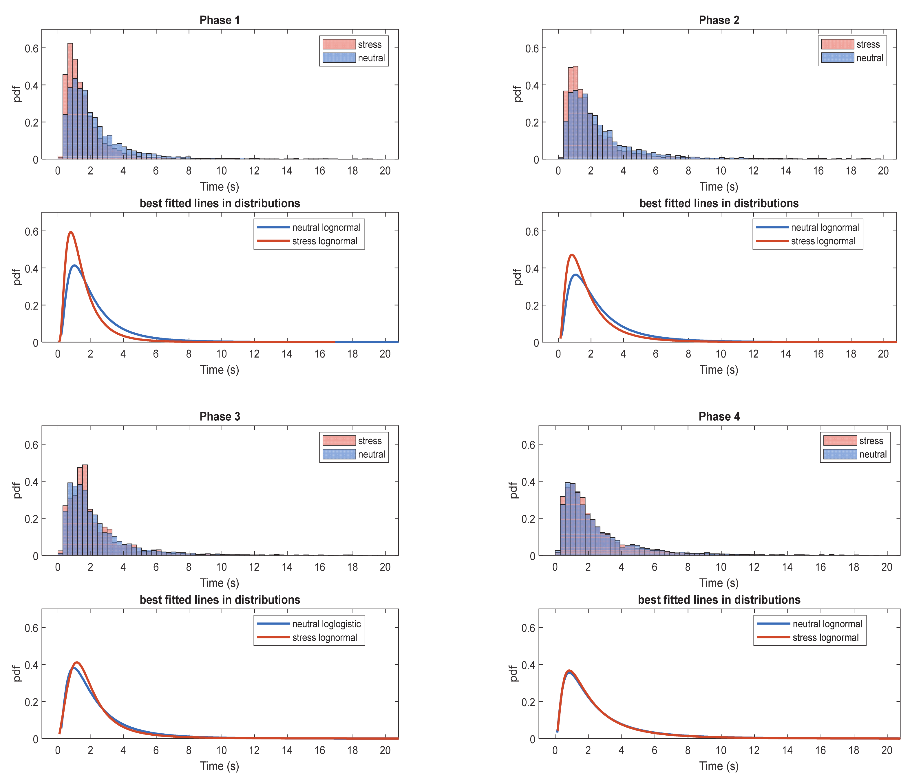
The normalized IBI histograms providing the probability density function (pdf) were extracted for each experimental task of the three datasets under investigation. The IBI histograms were grouped according to their experimental phase and induced affective state (neutral, stress). For each aggregated histogram, the best fitted distribution to the data was extracted among the candidate distributions (beta, exponential, gamma, logistic, log-logistic, lognormal, normal, Rayleigh, Weibull distributions). The aggregated IBI histograms for each experimental phase along with their best fitted distributions, are shown in Figure 3.

Inspecting the behaviour of the distribution for each task in Figure 3, it can be deduced that the stressful states (e.g., interview, emotional recall) distributions have offset to the right in relation to the stressful state for the first 2 phases. This can be partially attributed to the fact that during stress conditions eye blink rate increases. The best fitted distribution on each phase is lognormal in all cases except phase 3 neutral state which is log-logistic. All best-fitted distributions are presented in

Table 3. Best Fitted distribution and corresponding parameters (μ, σ or λ).

Experimental Task	Fitted Distribution	Parameters		Kolmogorov X2 Test
		μ	σ or λ
Social Exposure
Neutral (reference)	lognormal	0.54	0.74	↓
Stress (Interview, text reading)	lognormal	0.22	0.68
Emotional recall
Neutral (reference)	lognormal	0.65	0.77	↓
Stress (recall anxious/stressful event)	lognormal	0.39	0.76
Mental tasks
Neutral (reference)	loglogistic	0.59	0.80	↓
Stress (SCWT, images)	lognormal	0.54	0.43
Stressful videos
Calming video (reference)	lognormal	0.63	0.89	ns
Stress (stressful videos)	lognormal	0.60	0.87

↓/ns are significantly decreased and no significant changes during 2-samples Kolmogorov Smirnov test.

. The differentiation of distribution of IBI that each task follows for the dataset was checked using 2 samples Kolmogorov-Smirnov test [25].

It can be observed that in most cases the best-fitted distribution among the distributions described is the lognormal distribution. During the 3 out of 4 experimental phases (social exposure, emotional recall and mental tasks), the 2-sample Kolmogorov-Smirnov X² test revealed that the data of neutral and stress states come from different distributions. Then, it was investigated whether the IBI distributions present significant differences between the two emotional states (neutral, stress) for each experimental phase utilizing all the 3 available datasets. The IBI comparison was performed using the Z-test of two log-normal samples [26] and the results are shown in

Table 4. Two-sample log-normal Z-test for each experimental phase utilizing all the 3 available datasets.

Experimental Phase	Two-Sample Log-Normal Z-Score	p-Value	Z-Test
Social Exposure	21.84	<0.01	↓
Emotional recall	9.49	<0.01	↓
Mental tasks	2.33	<0.01	↓
Stressful videos	1.48	>0.05	ns

↓/ns are significantly decreased and no significant changes during 2-sample Z-test.

.

It can be observed, that during the social exposure, emotional recall and mental tasks a statistically significant difference between the neutral and stress state is present. Especially, during 2 of these phases (social exposure, emotional recall) significantly reduced IBI exists during stress compared to neutral states. These results indicate that during stress conditions there are increased blinks, as supported also in relevant literature [7,8].

4.2. Threshold Determination

Then, the pattern of eye blinks activity was investigated by employing Markov chains [27], described in Section 3.5. In Figure 4 the histogram of the calculated IBIs, for each experiment from all tasks (neutral, stressed and relaxed) is shown. The identification of the number of groups into which the IBIs can be differentiated is performed by visual inspection, but also by using the kernel density function on the histogram of all IBIs, as described in [28]. Two groups are finally selected for each of the three experiments. The time-point threshold for the two groups for the 1st, 2nd and 3rd experiment was 1.975 s, 2.325 s and 1.975 s respectively. The highest value of these three thresholds was used, namely 2.325 s. Accordingly, two states can be selected for the Markov Analysis, the “long” IBI state and the “short” IBI state.

4.3. Classification Performance

In

Table 5. The average classification accuracy, precision and recall between cognitive processes on the testing set after 10 runs. Values are averages over 10 trials.

Experimental Phase	Accuracy%	Precision%	Recall%
	CNN
Social exposure	50.4	49.3	74.0
Emotional recall	74.5	63.5	80.0
Mental tasks	76.4	74.5	80.0
Stressful videos	67.6	68.4	75.0
	LSTM
Social exposure	74.1	80.6	72.2
Emotional recall	65.7	84.6	66.2
Mental tasks	79.5	99.0	76.7
Stressful videos	64.3	86.1	68.0

, we depict the prediction models performance in discriminating stressed and neutral states, for each experimental phase using the sequence of IBIs or blinks sequences as input to the CNN and LSTM networks. 8 classifiers (4 CNN and 4 LSTM) were implemented, one for each experimental phase, comparing stressed and neutral tasks per cognitive process, the parameters of which are presented in Section 3.4. The IBI sequence per subject is fed into the network architecture. For the CNN classifier, the true positive rate (Recall) is greater than the positive predictive value (Precision). The opposite is observed for the LSTM classifier. Comparing the range of values across phases for the two classifiers, for the Precision and Recall metrics, the difference in performance for the Precision is most notable, the range for the CNN classifier being [49.3–74.5], while for the LSTM classifier being [80.6–99.0]. Having in mind that a “positive” classification result corresponds to classifiying a recording as belonging to a stressful task, while a “negative” classification result corresponds to classifying a recording as belonging to a neutral task, the results provide an indication that LSTM performs better than CNN when presented with recordings belonging to neutral tasks.

Furthermore, the best classification accuracy results are achieved for the mental tasks phase for both the CNN and the LSTM classifier, closely followed by the emotional recall phase for the CNN and the social exposure phase for the LSTM classifier. These findings might provide in turn indications that the blink generation under these processes/phases has different patterns. The patterns of blink generation were analyzed in this study using Markovian Analysis and the results are presented hereafter.

4.4. Markovian Analysis

The main feature used in order to capture the task dynamics is the IBI. By separating the IBIs distribution in two categories it is an open question whether the generation of blinks is subject to two attractor states, one in which blinks occur in a short time, resulting in short IBIs, and another in which blinks occur in a long time, resulting in long IBIs. These different states of blink generation during watching neutral, relax and stressful video was analyzed by applying first-order Markovian Analysis. The state transition probability matrices (STPMs) $P$ were calculated and compared with the $P^{\left(0\right)}$ matrices giving the probability of being at state $i$, in order to test whether the generation of blinks during relaxing/stress procedures is a stochastic process. The statistical significance between these two matrices was calculated and the results are presented in

Table 6. First order Markovian Analysis. State #1 (#2) corresponds to short (long) IBIs.

1st Experiment	Social Exposure	${\mathit{S}}_{\mathit{i}\mathit{j}}$	${\mathit{P}}_{\mathit{i}\mathit{j}}\left(95\mathit{\%} \mathit{c}\mathit{o}\mathit{n}\mathit{f}\mathit{i}\mathit{d}\mathit{e}\mathit{n}\mathit{c}\mathit{e} \mathit{i}\mathit{n}\mathit{t}\mathit{e}\mathit{r}\mathit{v}\mathit{a}\mathit{l}\right)$	${\mathit{P}}_{\mathit{i}\mathit{j}}^{\left(0\right)}$	${\mathit{X}}^2$
	Neutral				8.16
	1,1 S–S	150	0.81 [0.7754–0.8375]	0.78
	1,2 S–L	36	0.19 [0.1625–0.2246]	0.22
	2,1 L–S	32	0.60 [0.5488–0.6587]	0.77
	2,2 L–L	21	0.40 [0.3413–0.4512]	0.22
	Stressed				28.08
	1,1 S–S	441	0.77 [0.7572–0.7929]	0.75
	1,2 S–L	128	0.23 [0.2071–0.2428]	0.25
	2,1 L–S	123	0.65 [0.6234–0.6851]	0.75
	2,2 L–L	65	0.35 [0.3149–0.3766]	0.25
	Emotional recall
	Neutral				11.07
	1,1 S–S	105	0.77 [0.7365–0.8190]	0.69
	1,2 S–L	30	0.22 [0.1810–0.2635]	0.31
	2,1 L–S	26	0.43 [0.3707–0.4817]	0.69
	2,2 L–L	35	0.57 [0.5183–0.6293]	0.31
	Stressed				36.73
	1,1 S–S	288	0.79 [ 0.7727–0.8184]	0.76
	1,2 S–L	74	0.20 [0.1816–0.2273]	0.23
	2,1 L–S	65	0.61 [0.5788–0.6593]	0.76
	2,2 L–L	40	0.39 [0.3407–0.4212]	0.23
	Stressful images/Stroop task
	Stressed				24.57
	1,1 S–S	794	0.76 [0.7503–0.7781]	0.70
	1,2 S–L	245	0.24 [0.2219-0.2497]	0.30
	2,1 L–S	254	0.57 [0.5500–0.5915]	0.70
	2,2 L–L	191	0.43 [0.4085–0.4500]	0.30
	Stressful videos				120.54
	Neutral
	1,1 S–S	481	0.78 [0.7629–0.8014]	0.67
	1,2 S–L	134	0.22 [0.1986–0.2371]	0.33
	2,1 L–S	136	0.45 [0.4218–0.4759]	0.67
	2,2 L–L	167	0.55 [0.5241–0.5782]	0.33
	Stressed				35.29
	1,1 S–S	641	0.71 [0.6933–0.7265]	0.63
	1,2 S–L	262	0.29 [0.2735–0.3067]	0.37
	2,1 L–S	261	0.49 [0.4691–0.5103]	0.63
	2,2 L–L	272	0.51 [0.4897–0.5309]	0.37
2nd Experiment	Social Exposure
	Neutral				20.67
	1,1 S–S	256	0.74 [0.7134–0.7663]	0.66
	1,2 S–L	90	0.26 [0.2337–0.2866]	0.34
	2,1 L–S	86	0.48 [ 0.4397–0.5106]	0.66
	2,2 L–L	95	0.53 [ 0.4894–0.5603]	0.34
	Stressed				33.28
	1,1 S–S	642	0.86 [0.8484–0.8751]	0.84
	1,2 S–L	103	0.14 [0.1249–0.1516]	0.16
	2,1 L–S	97	0.70 [0.6712–0.7346]	0.84
	2,2 L–L	41	0.30 [0.2654–0.3288]	0.16
	Emotional recall
	Neutral				37.07
	1,1 S–S	311	0.78 [0.7564–0.8025]	0.69
	1,2 S–L	88	0.22 [0.1975–0.2436]	0.31
	2,1 L–S	87	0.49 [0.4600–0.5286]	0.69
	2,2 L–L	89	0.51 [0.4714–0.5400]	0.31
	Stressed				61.40
	1,1 S–S	583	0.76 [0.7419–0.7763]	0.72
	1,2 S–L	185	0.24 [0.2237–0.2581]	0.28
	2,1 L–S	186	0.51 [0.4845–0.5319]	0.72
	2,2 L–L	180	0.49 [0.4681–0.5155]	0.28
	Stressful images
	Stressed				187.99
	1,1 S–S	1163	0.78 [0.7648–0.7890]	0.69
	1,2 S–L	334	0.22 [0.2110–0.2352]	0.31
	2,1 L–S	343	0.52 [0.5002–0.5345]	0.69
	2,2 L–L	320	0.48 [0.4655–0.4998]	0.31
	Stressful videos				148.92
	Neutral
	1,1 S–S	772	0.76 [0.7471–0.7771]	0.65
	1,2 S–L	241	0.24 [0.2229–0.2529]	0.35
	2,1 L–S	240	0.44 [0.4191–0.4600]	0.65
	2,2 L–L	306	0.56 [0.5400–0.5809]	0.35
	Stressed				319.10
	1,1 S–S	1308	0.81 [0.8024–0.8255]	0.72
	1,2 S–L	299	0.19 [0.1745–0.1976]	0.28
	2,1 L–S	299	0.47 [0.4512–0.4876]	0.72
	2,2 L–L	338	0.53 [ 0.5124–0.5488]	0.28
3rd Experiment	Social Exposure
	Neutral				433.35
	1,1 S–S	2982	0.76 [0.7487–0.7635]	0.67
	1,2 S–L	962	0.24 [0.2365–0.2513]	0.33
	2,1 L–S	940	0.49 [0.4783–0.4993]	0.67
	2,2 L–L	983	0.51 [0.5007–0.5217]	0.33
	Stressed				63.22
	1,1 S–S	3129	0.86 [0.8488–0.8610]	0.83
	1,2 S–L	531	0.15 [0.1390–0.1512]	0.17
	2,1 L–S	538	0.73 [0.7113–0.7388]	0.83
	2,2 L–L	204	0.28 [0.2612–0.2887]	0.17
	Emotional recall
	Neutral				237.38
	1,1 S–S	1111	0.72 [0.7074–0.7388]	0.59
	1,2 S–L	392	0.28 [0.2662–0.2926]	0.41
	2,1 L–S	375	0.39 [0.3750–0.4079]	0.59
	2,2 L–L	583	0.61 [0.5921–0.6250]	0.41
	Stressed				238.21
	1,1 S–S	2129	0.82 [0.8158–0.8326]	0.76
	1,2 S–L	454	0.18 [0.1674–0.1842]	0.24
	2,1 L–S	447	0.56 [0.5451–0.5752]	0.76
	2,2 L–L	351	0.44 [0.4248–0.4549]	0.24
	Mental tasks
	Neutral				282.55
	1,1 S–S	1252	0.76 [0.7520–0.7757]	0.64
	1,2 S–L	387	0.24 [0.2243–0.2480]	0.36
	2,1 L–S	389	0.42 [0.4035–0.4358]	0.64
	2,2 L–L	538	0.58 [0.5642–0.5965]	0.36
	Stressed				441.19
	1,1 S–S	2823	0.77 [0.7576–0.7733]	0.67
	1,2 S–L	865	0.23 [0.2267–0.2424]	0.33
	2,1 L–S	870	0.48 [0.4651–0.4868]	0.67
	2,2 L–L	958	0.52 [0.5132–0.5349]	0.33
	Stressful videos
	Neutral				320.20
	1,1 S–S	1094	0.76 [0.7505–0.7764]	0.62
	1,2 S–L	339	0.24 [0.2236–0.2495]	0.38
	2,1 L–S	343	0.40 [0.3816–0.4142]	0.62
	2,2 L–L	519	0.60 [0.5858–0.6184]	0.38
	Stressed				384.25
	1,1 S–S	1979	0.72 [0.7134–0.7322]	0.61
	1,2 S–L	759	0.28 [0.2678–0.2866]	0.39
	2,1 L–S	762	0.43 [0.4185–0.4442]	0.61
	2,2 L–L	1009	0.57 [0.5580–0.5815]	0.39

.

In Table 6 the matrices $S, P, P^{\left(0\right)}, X^2$ are presented for each experiment, phase and task. Based on chi-square statistics with 2 degrees of freedom at $a=0.05$ significance level, P is significantly different from $P^{\left(0\right)}$ when the values of $X^2$ is larger than the value 5.991, based on chi-square distribution tables. This was the case for all tasks. Thus the null hypothesis that matrix P is equal to matrix $P^{\left(0\right)}$ was rejected and a first-order Markov process was assumed for all tasks. Therefore, it was conjectured that the process generating blinks possessed, at least, first-order “memory” in all tasks. For each original element value of the matrix P, a distribution of 1000 Bootstrap values was derived, and the 2.5% and 97.5% percentiles of this distribution were calculated and used as the 95% confidence interval for the particular original element value of the P matrix.

Furthermore, Table 6 shows that $P_{11}$ and $P_{22}$ are significantly higher than the corresponding $P_{11}^{\left(0\right)}$ and $P_{22}^{\left(0\right)}$, for all experiments, phases and tasks—except, marginally, for $P_{11}$ for experiment 1, social exposure phase, neutral task—while $P_{12}$ and $P_{21}$ are significantly lower than the corresponding $P_{12}^{\left(0\right)}$ and $P_{21}^{\left(0\right)}$, based on their 95% confidence intervals as presented in Table 6. These results provide an indication that state 1 and state 2 can be characterized as “auto-attractors”, meaning that the blink generation system has a tendency to either maintain short IBIs (state 1) or long IBIs (state 2), while avoiding transitions from one state to the other. In order to investigate furthermore the indications about the existence of auto-attractor states, looking at differences within matrix P, it was observed that $P_{11}$ was significantly higher than $P_{12}$ for all experiments, phases and tasks. On the other hand, $P_{22}$ was significantly higher than $P_{21}$ for both tasks of the stressful video phase of experiments 2 and 3, for both tasks of the mental tasks phase of experiment 3, while for experiment 1 $P_{22}$ was significantly higher than $P_{21}$ for the neutral tasks of the emotional recall and stresfull video phases. Thus, the evidence that state 1 is an auto-attractor in all experiments, phases and tasks (keeping in mind the exception for one task, stated above) is strengthened. On the other hand, the nature of state 2 as an auto-attractor seems to hold mainly for the stressful video phase (for both tasks) for experiments 2 and 3.

In conclusion, the generation of blinks seems not to be a purely random process. Instead, it appears to possess “memory”, in the sense that the previous state of the system (i.e., whether a short or long IBI preceded the current IBI) influences which will be the current state. Furthermore, there are strong indications that the short IBI state (state 1) can be characterized as an auto-attractor, across experiments, phases and tasks. Indications on whether the long IBI state (state 2) can be characterized as an auto-attractor across experiments and tasks seem to hold strongly for only the stressful videos phase. The preponderance of the short IBIs states over the long IBIs states, possibly in line with the indications that state 1 is an auto-attractor, is ascertained by the fact that $P_{11}$ is greater than $P_{22}$ for every task. Taking into account the finding that the auto-attractor nature of the short IBIs state exists for both the relaxation and the stress-inducing tasks and since stress has been shown to induce higher BR (therefore shorter IBIs), it would be interesting to further investigate whether the short IBI state, during which a subject produces relatively many blinks in sequence during the task, corresponds to an intra-task differentiation of stress levels, even for relaxation-inducing tasks.

As a further step of investigating the Markov dynamics of states 1 and 2, we compared the percentages of difference between $P_{ii}$ and $P_{ii}^{\left(0\right)}$, i = 1,2 between neutral and stressful tasks in the various phases. A higher percentage of difference for one task compared to the other, for a given state, might provide an indication that the attractor nature of that state is stronger for the task where the percentage is greater. The aim of the investigation was whether there existed a trend across experiments and phases, “linking” attractor states to neutral or stressful tasks. According to the above rationale, in the social exposure phase and emotional recall phase (except from experiment 2), the percentage of difference between $P_{11}$ and $P_{11}^{\left(0\right)}$ is greater in neutral than in stressed tasks, while, conversely, in the stressful videos phase the percentage of the difference between $P_{22}$ and $P_{22}^{\left(0\right)}$ is greater in stressed than in neutral tasks. In the emotional recall phase the same occurs in the 1st and 2nd experiment. For the mental task phase and the stressful videos phase, in the 3rd experiment, the percentage of difference between $P_{11}$ and $P_{11}^{\left(0\right)}$ and $P_{22}$ and $P_{22}^{\left(0\right)}$ is greater in neutral than in stressed tasks. Additionally, for the stressful videos phase, in experiment 2, the percentage of the difference between $P_{11}$ and $P_{11}^{\left(0\right)}$ is greater in neutral than in stressed tasks, while the percentage of the difference between $P_{22}$ and $P_{22}^{\left(0\right)}$ is greater in stressed than in neutral tasks.

It was mentioned above that the rate of blink generation is increasing under stressed tasks, so the “short” attractor (#1) could be expected to be strongest in stressed tasks, while, in contradistinction, the “long” attractor (#2) is expected to be strongest in the neutral tasks. This expectation was not verified across all the experiments based on the Markovian Analysis presented above. In order to investigate the impact of the attractor’s existence on the classification accuracy, further analyses were implemented. Specifically, for each phase, we selected the experiment that presented concurrently the strongest attractor values, as indicated by the percentage difference between values $P_{11}$ and $P_{11}^{\left(0\right)}$ (denoted $d{P}_{11}{\left(\%\right)}_s$ in the following), as well as between $P_{22}$ and $P_{22}^{\left(0\right)}$ (denoted $d{P}_{22}{\left(\%\right)}_n$ in the following), under stressed and neutral tasks, respectively, and then trained, per phase, the classifiers using only the subjects from the selected experiment. As far as the classifier structure and classification testing are concerned, the hyperparameters of the 1D CNN architecture and LSTM classifier remained the same. The nested cross-validation scheme was selected to 3 × 5 after trial-error investigation. The classification results are presented in

Table 7. The average classification accuracy between cognitive processes on the testing set after 10 runs. Values are averages over 10 trials.

Experimental Phase/Experiment	Accuracy CNN (3 × 5 CV)	Accuracy LSTM (3 × 5 CV)
Social Exposure/Experiment 1	72.7%	81.3%

.

Specifically, in the social exposure phase under stressed tasks $d{P}_{11}{\left(\%\right)}_s$ is strongest in experiments 1 and 3 (3%), while $d{P}_{22}{\left(\%\right)}_n$ in the social exposure phase under neutral tasks is strongest in experiment 1 (79%). So the experiment for which both $d{P}_{11}{\left(\%\right)}_s$ and $d{P}_{22}{\left(\%\right)}_n$ reached their peaks was experiment 1. Therefore, the IBI sequences of experiment 1 were fed into the classifiers (CNN and LSTM). For the other phases, the application of the above methodology did not lead to a selection of one specific experiment, since, as exposed hereafter, $d{P}_{11}{\left(\%\right)}_s$ and $d{P}_{22}{\left(\%\right)}_n$ had peaks at different experiments. For the emotional recall phase, experiment 1 presents the strongest $d{P}_{22}{\left(\%\right)}_n$ (84%), while $d{P}_{11}{\left(\%\right)}_s$ is strongest in experiment 2 (12%). For the stressful images phase, which has only a stress producing task and the neutral task used for comparison is the neutral task of the emotional recall phase, $d{P}_{11}{\left(\%\right)}_s$ is strongest in experiment 2 (12%), while $d{P}_{22}{\left(\%\right)}_n$ is strongest for experiments 1 (84%). Additionally, since the mental task phase was present only in experiment 3 the proposed methodology was not applied for this phase. Finally, for the stressful videos phase $d{P}_{11}{\left(\%\right)}_s$ is strongest n experiment 1 (19%), while $d{P}_{22}{\left(\%\right)}_n$ is strongest in experiment 1 (67%).

As can be seen from Table 7 there is a notable improvement for the classification accuracy for the social exposure phase, for both the CNN and the LSTM classifier, when data were used only from experiment 1, according to the methodological criteria stated above. Of note is also the fact that the classification accuracy reached for the LSTM classifier is highest than any accuracy value reached when data from all experiments were used concurrently, as presented in Table 5.

5. Discussion

The aim of this study is the investigation of blinks patterns as manifested in the IBI sequences produced during neutral and stress conditions, provided by experimental tasks related to social exposure, emotional recall and cognitive processes.

The IBIs appear to follow log-normal distribution in the vast majority of experimental tasks for the three available datasets. The distributions corresponding to neutral and stress conditions appear to be different in 3 out of 4 experimental phases (social exposure, emotional recall and mental tasks). Especially, during the social exposure and emotional recall phases, the stress has an effect the concentration of significantly more short IBIs. This pattern seems to be consistent along the three different datasets, representing an interesting finding, indicating that during stress conditions there are increased blinks.

Then, we explored classification of stressed and neutral tasks on different cognitive tasks using deep CNN architectures and Markov Chain. Although CNN has been applied widely on blink detection [29,30], to our knowledge, it is the first time that inter-blink interval is analyzed with both CNN and Markov Chain models, with the aim of investigating both the existence of differentiation between the two stress-related categories of tasks and more in-depth state relationships as can be revealed by Markov Analysis. By combining data from all the experiments, the best CNN model in the present study achieved 76.4% testing accuracy for the mental tasks phase, while the LSTM network 79.5% for the same experimental phase. The use of Markovian Analysis, for selecting data from experiments where the “attractor” states were stronger improved notably the classification accuracy (81%). Future work would be the detection of the stress level using the IBI sequence, as many studies have been shown high accuracies on recognizing levels of psychological stress, e.g., stress level can be automatically recognized by analyzing ECG signals in a multi-modal fusion and respiratory signals [31,32,33] with high accuracy.

Markov Analysis provided statistically significant indications that the blink generation is not purely random but depends on the history of previous blinks occurrences, implying the presence of memory in the system generating the blinks. We showed that, if the IBI sequence is modeled as a first-order Markov Chain, the generation of blinks during stressful and neutral cognitive possesses characteristics according to which the duration of a particular IBI depends significantly on the duration of the immediately previous IBI. If the occurrence of blinks were purely random, then one would expect that the occurrence of a given IBI would follow a renewal process, meaning that the IBI would be independent of previous IBIs. That was shown not to be the case, implying that the blink generation was not purely random. Moreover, the above findings were observed for the generation of blinks in all three experiments and four cognitive process for both tasks, neutral and stressed.

Our detailed analysis of matrices P and $P^{\left(0\right)},$ given the assumption of a first-order Markov process, provided further insight into the possible mechanism of blink generation. Given a short IBI, a tendency to repeat a short IBI was shown. Moreover, given a long IBI, a tendency to repeat a long IBI was shown well, albeit in a more nuanced way than the trend concerning short IBIs. Therefore, our analysis provided evidence that the system of blink generation may operate in two ‘‘attractor” states, one in which blinks occur at short consecutive IBIs and one in which blinks occur at long consecutive IBIs. Furthermore, we found that the short IBI attractor state characteristic existed in all cognitive tasks, suggesting that this mechanism does not depend on the particular task demands. Similar attractor behavior has been shown in a previous study [28], investigating the inter-saccadic intervals under fixation tasks. In addition, the evidence that the generation of blinks during different procedures is not a random process may induce the research community on a better understanding of the brain functioning.

References

1. Bulling, A. Eye Movement Analysis for Context Inference and Cognitive-Awareness: Wearable Sensing and Activity Recognition Using Electrooculography; Lulu Press: Morrisville, NC, USA, 2010. [Google Scholar]
2. Search BioNumbers—The Database of Useful Biological Numbers, Harvard. Available online: https://bionumbers.hms.harvard.edu/search.aspx (accessed on 15 September 2020).
3. Ousler, G.W., III; Hagberg, K.W.; Schindelar, M.; Welch, D.; Abelson, M.B. The ocular protection index. Cornea 2008, 27, 509–513. [Google Scholar] [CrossRef]
4. Giannakakis, G.; Grigoriadis, D.; Giannakaki, K.; Simantiraki, O.; Roniotis, A.; Tsiknakis, M. Review on psychological stress sdetection using biosignals. IEEE Trans. Affect. Comput. 2019. [Google Scholar] [CrossRef]
5. Laretzaki, G.; Plainis, S.; Vrettos, I.; Chrisoulakis, A.; Pallikaris, I.; Bitsios, P. Threat and trait anxiety affect stability of gaze fixation. Biol. Psychol. 2011, 86, 330–336. [Google Scholar] [CrossRef] [PubMed]
6. Maffei, A.; Angrilli, A. Spontaneous blink rate as an index of attention and emotion during film clips viewing. Physiol. Behav. 2019, 204, 256–263. [Google Scholar] [CrossRef] [PubMed]
7. Haak, M.; Bos, S.; Panic, S.; Rothkrantz, L. Detecting stress using eye blinks and brain activity from EEG signals. In Proceeding of the 1st Driver Car Interaction and Interface (DCII 2008), Prague, Czech Republic, 3–4 December 2008; pp. 35–60. [Google Scholar]
8. Giannakakis, G.; Pediaditis, M.; Manousos, D.; Kazantzaki, E.; Chiarugi, F.; Simos, P.; Marias, K.; Tsiknakis, M. Stress and anxiety detection using facial cues from videos. Biomed. Signal Process. 2017, 31, 89–101. [Google Scholar] [CrossRef]
9. Caffier, P.P.; Erdmann, U.; Ullsperger, P. Experimental evaluation of eye-blink parameters as a drowsiness measure. Eur. J. Appl. Physiol. 2003, 89, 319–325. [Google Scholar] [CrossRef]
10. Stroop, J.R. Studies of interference in serial verbal reactions. J. Exp. Psychol. 1935, 18, 643. [Google Scholar] [CrossRef]
11. Gronwall, D. Paced auditory serial-addition task: A measure of recovery from concussion. Percept. Motor Skills 1977, 44, 367–373. [Google Scholar] [CrossRef]
12. Lang, P.J.; Bradley, M.M.; Cuthbert, B.N. International affective picture system (IAPS): Technical manual and affective ratings. NIMH Cent. Study Emot. Atten. 1997, 39–58. [Google Scholar]
13. Andreu, Y.; Chiarugi, F.; Colantonio, S.; Giannakakis, G.; Giorgi, D.; Henriquez, P.; Kazantzaki, E.; Manousos, D.; Marias, K.; Matuszewski, B.J.; et al. Wize Mirror—A smart, multisensory cardio-metabolic risk monitoring system. Comput. Vis. Image Underst. 2016, 148, 3–22. [Google Scholar] [CrossRef] [Green Version]
14. Viola, P.; Jones, M.J. Robust real-time face detection. Int. J. Comput. Vis. 2004, 57, 137–154. [Google Scholar] [CrossRef]
15. Matthews, I.; Baker, S. Active appearance models revisited. Int. J. Comput. Vis. 2004, 60, 135–164. [Google Scholar] [CrossRef] [Green Version]
16. Castellanos, N.P.; Makarov, V.A. Recovering EEG brain signals: Artifact suppression with wavelet enhanced independent component analysis. J. Neurosci. Methods 2006, 158, 300–312. [Google Scholar] [CrossRef] [PubMed]
17. Doughty, M.J. Further assessment of gender-and blink pattern-related differences in the spontaneous eyeblink activity in primary gaze in young adult humans. Optom. Vis. Sci. 2002, 79, 439–447. [Google Scholar] [CrossRef]
18. Ponder, E.; Kennedy, W. On the act of blinking. Q. J. Exp. Physiol. Transl. Integr. 1927, 18, 89–110. [Google Scholar] [CrossRef]
19. Bacivarov, I.; Ionita, M.; Corcoran, P. Statistical models of appearance for eye tracking and eye-blink detection and measurement. IEEE Trans. Consum. Electron. 2008, 54, 1312–1320. [Google Scholar] [CrossRef] [Green Version]
20. Kingma, D.P.; Ba, J. Adam: A method for stochastic optimization. arXiv 2014, arXiv:1412.6980. [Google Scholar]
21. Chollet, F. Keras: Deep Learning Library for Theano and Tensorflow. Available online: https://keras.io/k (accessed on 15 September 2020).
22. Abadi, M.; Agarwal, A.; Barham, P.; Brevdo, E.; Chen, Z.; Citro, C.; Corrado, G.S.; Davis, A.; Dean, J.; Devin, M. Tensorflow: Large-scale machine learning on heterogeneous distributed systems. arXiv 2016, arXiv:1603.04467. [Google Scholar]
23. Karim, F.; Majumdar, S.; Darabi, H.; Harford, S. Multivariate LSTM-FCNs for time series classification. Neural Netw. 2019, 116, 237–245. [Google Scholar] [CrossRef] [Green Version]
24. Anderson, T.W.; Goodman, L.A. Statistical inference about Markov chains. Ann. Math. Stat. 1957, 28, 89–110. [Google Scholar] [CrossRef]
25. Massey, F.J., Jr. The Kolmogorov-Smirnov test for goodness of fit. J. Am. Stat. Assoc. 1951, 46, 68–78. [Google Scholar] [CrossRef]
26. Zhou, X.-H.; Gao, S.; Hui, S.L. Methods for comparing the means of two independent log-normal samples. Biometrics 1997, 53, 1129–1135. [Google Scholar] [CrossRef] [PubMed]
27. Ktonas, P.; Bes, F.; Rigoard, M.; Wong, C.; Mallart, R.; Salzarulo, P. Developmental changes in the clustering pattern of sleep rapid eye movement activity during the first year of life: A Markov-process approach. Electroencephalogr. Clin. Neurophysiol. 1990, 75, 136–140. [Google Scholar] [CrossRef]
28. Korda, A.I.; Koliaraki, M.; Asvestas, P.A.; Matsopoulos, G.K.; Ventouras, E.M.; Ktonas, P.Y.; Smyrnis, N. Discrete states of attention during active visual fixation revealed by Markovian analysis of the time series of intrusive saccades. Neuroscience 2016, 339, 385–395. [Google Scholar] [CrossRef] [PubMed]
29. Garg, P.; Davenport, E.; Murugesan, G.; Wagner, B.; Whitlow, C.; Maldjian, J.; Montillo, A. Using convolutional neural networks to automatically detect eye-blink artifacts in magnetoencephalography without resorting to electrooculography. In Proceedings of the Medical Image Computing and Computer Assisted Intervention (MICCAI 2017), Quebec City, QC, Canada, 11–13 September 2017. [Google Scholar]
30. Kim, K.W.; Hong, H.G.; Nam, G.P.; Park, K.R. A Study of Deep CNN-Based Classification of Open and Closed Eyes Using a Visible Light Camera Sensor. Sensors 2017, 17, 1534. [Google Scholar] [CrossRef] [PubMed] [Green Version]
31. Rastgoo, M.N.; Nakisa, B.; Maire, F.; Rakotonirainy, A.; Chandran, V. Automatic driver stress level classification using multimodal deep learning. Expert Syst. Appl. 2019, 138, 112793. [Google Scholar] [CrossRef]
32. Shan, Y.; Li, S.; Chen, T. Respiratory signal and human stress: Non-contact detection of stress with a low-cost depth sensing camera. Int. J. Mach. Learn. Cybern. 2020, 11, 1825–1837. [Google Scholar] [CrossRef]
33. Giannakakis, G.; Trivizakis, E.; Tsiknakis, M.; Marias, K. A novel multi-kernel 1D convolutional neural network for stress recogni-tion from ECG. In Proceedings of the 2019 8th International Conference on Affective Computing and Intelligent Interaction Work-shops and Demos (ACIIW), Cambridge, UK, 3–6 September 2019; pp. 1–4. [Google Scholar]
Figure 1. Schematic representation of the eye aperture timeseries extraction. The 68 2D facial landmarks (blue dots) were extracted from facial videos using AAM (left image). Each eyeball perimeter was segmented by 6 discrete landmarks. The eye aperture is provided by the shaded blue area (right upper image) and a typical eye aperture timeseries is shown in the right lower graph.
Signals 02 00006 g001
Figure 2. Time series of eye aperture and the identified blink peaks (denoted with red points). The IBI and the blink duration are also illustrated.
Signals 02 00006 g002
Figure 3. Normalized histograms of IBI for each experimental phase (phase 14) and induced affective state (neutral blue, stress red) and the corresponding best fitted distribution.
Signals 02 00006 g003
Figure 4. The blue line represents the kernel density estimator of the distribution of IBIs. The red line represents the second derivative of the kernel density estimator. The threshold for dividing the two states (short and long IBIs) is taken to be the IBI value (indicated by the square) that corresponds to the largest peak in the second derivative curve (indicated by square), which is to the right of the maximum of the kernel density curve. (ac) correspond to the 1st, 2nd and 3rd experiment, respectively.
Signals 02 00006 g004aSignals 02 00006 g004b